Applied Thermal Engineering 29 (2009) 3036–3048

Contents lists available at ScienceDirect

Applied Thermal Engineering

journal homepage: www.elsevier .com/locate /apthermeng

The experimental validation of a simplified PEMFC simulation model for designand optimization purposes

L.S. Martins a, J.E.F.C. Gardolinski b, J.V.C. Vargas b,*, J.C. Ordonez a, S.C. Amico c, M.M.C. Forte c

a Department of Mechanical Engineering and Center for Advanced Power Systems, Florida State University, Tallahassee, FL 32310-6046, USAb Departamento de Engenharia Mecânica, Universidade Federal do Paraná, C. P. 19011, Curitiba, Paraná 81531-990, Brazilc Laboratório de Materiais Poliméricos, Departamento de Materiais, Universidade Federal do Rio Grande do Sul, C. P. 15010, Porto Alegre, Rio Grande do Sul 91501-970, Brazil

a r t i c l e i n f o a b s t r a c t

Article history:Received 8 December 2007Accepted 1 April 2009Available online 8 April 2009

Keywords:PEMFC experimental measurementsNumerical simulationInfrared imagingPEMFC net power output

1359-4311/$ - see front matter � 2009 Elsevier Ltd. Adoi:10.1016/j.applthermaleng.2009.04.002

* Corresponding author. Tel.: +55 41 3361 3307; faE-mail address: jvargas@demec.ufpr.br (J.V.C. Varg

Geometric design, including the internal structure and external shape, considerably affect the thermal,fluid and electrochemical characteristics of a polymer electrolyte membrane fuel cell (PEMFC), whichdetermines the polarization curves as well as the thermal and net power responses. In order to predictthe response of PEM fuel cells according to the variation of manufacturing materials physical properties,operating and design parameters, a reliable simulation model (and computationally fast) is necessary,which accounts for the power losses due to pressure drops in the gas channels. In this paper, a simplifiedand comprehensive PEMFC mathematical model introduced in previous studies is experimentally vali-dated. Numerical results are obtained with the model for an existing set of ten commercial unit PEM fuelcells. The model accounts for pressure drops in the gas channels, and for temperature gradients withrespect to space in the flow direction, and current increase that are investigated by direct infrared imag-ing, showing that even at low current operation such gradients are present in fuel cell operation, andtherefore should be considered by a PEMFC model, since large coolant flow rates are limited due toinduced high pressure drops in the cooling channels. The computed polarization and power curves aredirectly compared to the experimentally measured ones with good qualitative and quantitative agree-ment. The combination of accuracy and low computational time allow for the future utilization of themodel as a reliable tool for PEMFC simulation, control, design and optimization purposes.

� 2009 Elsevier Ltd. All rights reserved.

1. Introduction

Fuel cell technology is well advanced, with applications in sta-tionary power generation and in vehicles [1–4]. Political effortsto reduce greenhouse gases in the road transport sector are basi-cally in conflict with the ever growing demand for transport ser-vices; emissions from internal combustion (IC) engines in theautomotive application have already been subject to increasinglytougher statutory limits for quite some time [5].

In recent years, considerable funds and research resources havebeen invested in developing the fuel cell as a source of electricalenergy to power vehicles, simultaneously to achieve the require-ments of significant reduction of engine CO2 emissions and pollu-tant emission free operation [6,7].

As a promising technology that may successfully supersede thecombustion of fossil fuel as the dominant method of energy con-version, hydrogen fuel cells are studied worldwide with an aimto improve the power output, lower the cost and extend the lifeof operation for widespread applications [8]. Fuel cells are ex-

ll rights reserved.

x: +55 41 3361 3129.as).

pected to be of practical use because they emit less environmentalpollutant and convert more efficiently from chemical energy toelectrical energy than other energy resources; especially, polymerelectrolyte membrane fuel cell (PEMFC) is expected to be the driv-ing power of vehicles and stationary power supply, because it canwork at low temperature and has high power density [9,10].

No other energy generation technology offers the combinationof benefits that fuel cells do. In addition to low or zero emissions,benefits include high efficiency and reliability, multi-fuel capabil-ity, sitting flexibility, durability, and ease of maintenance. Fuel cellsare also scalable and can be stacked until the desired power outputis reached. Since fuel cells operate silently, they reduce noise pol-lution as well as air pollution and the waste heat from a fuel cellcan be used to provide hot water or space heating for a home oroffice.

Technically and economically, there are still many hurdles to beovercome in fuel cell development before wide spread application.Modeling and computational simulation in one, two and threedimensions have been developed in academia and industry to as-sess the effect of materials, geometric and operating design param-eters on fuel cell response [9–20]. The results show that issues ashigh cost of materials, durability, water management and

Nomenclature

A area, m2

Ac total gas channel cross-section area, m2

As unit fuel cell cross-section area, m2

~A dimensionless areaB dimensionless constantBa bias limit of quantity ac specific heat, kmol kg�1 K�1

cp specific heat at constant pressure, kJ kg�1 K�1

C constant, Eq. (12)CV control volumeD Knudsen diffusion coefficient, m2 s�1

Dh gas channel hydraulic diameter, mf friction factorF Faraday constant, 96,500 Ceq�1

h heat transfer coefficient, W m�2 K�1

~h dimensionless heat transfer coefficientHi (Ti) molar enthalpy of formation at temperature Ti of reac-

tants and products, kJ kmol�1 of compound i~HiðhiÞ dimensionless molar enthalpy of formation at dimen-

sionless temperature hi of reactants and productsio,a, io,c exchange current densities, A m�2

iLim,a, iLim,c limiting current densities, A m�2

I current, A~I dimensionless currentj mass flux, kg m2 s�1

k thermal conductivity, W m�1 K�1

K permeability~k dimensionless thermal conductivityL control volume length, mLc, Lt gas channels internal dimensions as shown in Fig. 1, mLx, Ly, Lz fuel cell length, width and height, respectively, mm mass, kg_m mass flow rate, kg s�1

M molar weight, kg kmol�1

N equivalent electron per mole of reactant, eq mol�1

_n molar flow rate, kmol s�1

nc number of parallel ducts in gas channelN dimensionless global wall heat transfer coefficientp pressure, N m�2

~ps perimeter of cross-section, mPa precision limit of quantity aPEMFC polymer electrolyte membrane fuel cellPr Prandtl number, lcp/kq tortuosityQ reaction quotient_Q heat transfer rate, W~Q dimensionless heat transfer rater pore radius, mR ideal gas constant, kJ kg�1 K�1

�R universal gas constant, 8.314 kJ kmol�1 K�1

ReDh Reynolds number based on Dh, uDhq/lS dimensionless conversion factor, Eq. (41)T temperature, Ku mean velocity, m s�1

~u dimensionless mean velocityU global wall heat transfer coefficient, W m�2 K�1

Ua uncertainty of quantity aV electrical potential, VV volume, m3

VT total volume, m3

w weight, NW electrical work, J~W dimensionless fuel cell total electrical power~Wref dimensionless fuel cell net power~Wp dimensionless required pumping power

x axial direction, Fig. 1y2,4,6 size constraints½�� molar concentration of a substance, mol l�1

Greek symbolsaa, ac anode and cathode charge transfer coefficientsb electrical resistance, Xd gas channel aspect ratioDG molar Gibbs free energy change, kJ kmol�1 H2

D~G dimensionless molar Gibbs free energy changeDH molar enthalpy change, kJ kmol�1 H2

D~H dimensionless molar enthalpy changeDS molar entropy change, kJ kmol�1

DT temperature change, Kf stoichiometric ratioga, gc anode and cathode charge transfer overpotentials, Vgd,a, gd,c anode and cathode mass diffusion overpotentials, V~ga; ~gc dimensionless anode and cathode charge transfer over-

potentials~gd;a; ~gd;c dimensionless anode and cathode mass diffusion over-

potentials~gohm dimensionless fuel cell total ohmic potential lossh dimensionless temperaturek ionomer water contentl viscosity, kg m�1 s�1

ti reaction coefficientn dimensionless lengthq density, kg m�3

r electrical conductivity, X�1 m�1

/ porosityw dimensionless mass flow rate

SubscriptsA anode(aq) aqueous solutionc cathodedry drye reversiblef fuel(g) gaseous phaseH+ hydrogen cationH2 hydrogenH2O wateri irreversiblei,a irreversible at the anodei,c irreversible at the cathodein control volume inletload adjustable electrical load, Fig. 3b(l) liquid phasem maximum with respect to fuel cell internal structuremm maximum with respect to fuel cell internal an external

structureohm ohmicopt optimal valueout control volume outletox oxidantO2 oxygenp polymer electrolyte membraneref reference levels, a anode solid sides, c cathode solid sidesol solutionw wallwet wetted0 initial condition

L.S. Martins et al. / Applied Thermal Engineering 29 (2009) 3036–3048 3037

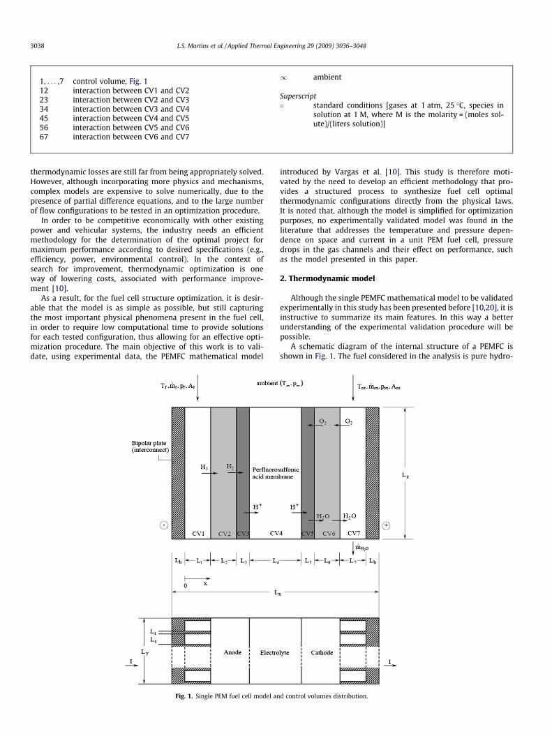
1, . . . ,7 control volume, Fig. 112 interaction between CV1 and CV223 interaction between CV2 and CV334 interaction between CV3 and CV445 interaction between CV4 and CV556 interaction between CV5 and CV667 interaction between CV6 and CV7

1 ambient

Superscript� standard conditions [gases at 1 atm, 25 �C, species in

solution at 1 M, where M is the molarity = (moles sol-ute)/(liters solution)]

3038 L.S. Martins et al. / Applied Thermal Engineering 29 (2009) 3036–3048

thermodynamic losses are still far from being appropriately solved.However, although incorporating more physics and mechanisms,complex models are expensive to solve numerically, due to thepresence of partial difference equations, and to the large numberof flow configurations to be tested in an optimization procedure.

In order to be competitive economically with other existingpower and vehicular systems, the industry needs an efficientmethodology for the determination of the optimal project formaximum performance according to desired specifications (e.g.,efficiency, power, environmental control). In the context ofsearch for improvement, thermodynamic optimization is oneway of lowering costs, associated with performance improve-ment [10].

As a result, for the fuel cell structure optimization, it is desir-able that the model is as simple as possible, but still capturingthe most important physical phenomena present in the fuel cell,in order to require low computational time to provide solutionsfor each tested configuration, thus allowing for an effective opti-mization procedure. The main objective of this work is to vali-date, using experimental data, the PEMFC mathematical model

Fig. 1. Single PEM fuel cell model an

introduced by Vargas et al. [10]. This study is therefore moti-vated by the need to develop an efficient methodology that pro-vides a structured process to synthesize fuel cell optimalthermodynamic configurations directly from the physical laws.It is noted that, although the model is simplified for optimizationpurposes, no experimentally validated model was found in theliterature that addresses the temperature and pressure depen-dence on space and current in a unit PEM fuel cell, pressuredrops in the gas channels and their effect on performance, suchas the model presented in this paper.

2. Thermodynamic model

Although the single PEMFC mathematical model to be validatedexperimentally in this study has been presented before [10,20], it isinstructive to summarize its main features. In this way a betterunderstanding of the experimental validation procedure will bepossible.

A schematic diagram of the internal structure of a PEMFC isshown in Fig. 1. The fuel considered in the analysis is pure hydro-

d control volumes distribution.

L.S. Martins et al. / Applied Thermal Engineering 29 (2009) 3036–3048 3039

gen, but it is possible to use a diluted hydrogen mixture generatedfrom a hydrocarbon reformation process. Although pure oxygen isassumed in the analysis, air could be used as the oxidant in theexperimental validation, provided that enough O2 is supplied tothe cell to meet the amount of oxygen required by the hydrogensupplied to the cell for a complete reaction.

The fuel cell is divided into seven control volumes that interactenergetically with one another. The fuel cell also interacts withadjacent fuel cells in a package, and or with the ambient. Addition-ally, two bipolar plates (interconnects) are presented: these havethe function of allowing the electrons produced by the electro-chemical oxidation reaction at the anode to flow to the externalcircuit or to an adjacent cell. The control volumes (CV) are fuelchannel (CV1), the anode diffusion-backing layer (CV2), the anodereaction layer (CV3), the polymer electrolyte membrane (CV4), thecathode reaction layer (CV5), the cathode diffusion-backing layer(CV6) and the oxidant channel (CV7).

The model consists of the conservation equations for each controlvolume, and the equations accounting for electrochemical reactions,where reactions are present. The reversible electrical potential andpower of the fuel cell are then computed (based on the reactions)as functions of the temperature and pressure fields determined bythe model. The actual electrical potential and power of the fuel cellare obtained by subtracting from the reversible potential the lossesdue to surface overpotentials (poor electrocatalysis), slow diffusionand all internal ohmic losses through the cell (resistance of individ-ual cell components, including electrolyte layer, interconnects andany other cell components through which electrons flow). Theseare functions of the total cell current (I), which is directly relatedto the external load (or the cell voltage). In sum, the total cell currentis considered an independent variable in this study.

2.1. Dimensionless variables

Dimensionless variables are defined based on the geometric andoperating parameters of the system. Pressures and temperaturesare referenced to ambient conditions Pi = pi/p1 and hi = Ti/T1.Dimensionless variables are defined as:

w ¼_mi

_mrefð1Þ

Ni ¼UwiV

2=3T

_mref cp;f; ~Ai ¼

Ai

V2=3T

ð2Þ

where subscript i indicates a substance or a location in the fuel cell.The fixed length scale V1=3

T is used for the purpose of non-dimensionalizing all the lengths that characterize the fuel cellgeometry,

nj ¼Lj

V1=3T

ð3Þ

where the subscript j indicates a particular dimension of the fuelcell geometry, Fig. 1.

~h ¼ hV2=3T

_mref cp;f; ~k ¼ kV1=3

T

_mref cp;fð4Þ

The physics of the fuel cell is described by taking into account themass conservation and the first law of thermodynamics at eachCV, and the electrochemical reactions at CV3 and CV5.

2.2. Mass balance

The hydrogen mass flow rate required for the current (I) dic-tated by the external load is

_mH2 ¼ _nH2 MH2 ¼I

nFMH2 ð5Þ

Therefore, the oxygen mass flow rate needed for a PEM fuel cell is

_mO2 ¼12

_nH2 MO2 ð6Þ

Stoichiometric ratios greater than 1 need be prescribed on the fuelside (f1) and oxidant side (f7).

2.3. Energy conservation

The wall heat transfer area of one control volume isAwi ¼ ~psLið2 � i � 6Þ and Awi ffi ~psLi þ LyLz (i = 1,7; assuming thatLt << Lc in Fig. 1), where ~ps ¼ 2ðLy þ LzÞ is the perimeter of the fuelcell cross-section. The control volumes are Vj = LyLzLj (2 6 j 6 6) andVj = ncLcLlLz (j = 1, 7), where nc is the integer part of Ly/(Lt + Lc), i.e.,the number of parallel ducts in each gas channel (fuel and oxidant).

The fuel pressure (pf in CV1) and oxidant pressure (pox in CV7)are assumed known and constant during fuel cell operation. Thestoichiometric ratio for an electrode reaction is defined as the pro-vided reactant (mol s�1) divided by the reactant needed for theelectrochemical reaction of interest. The mass and energy balancesfor CV1 yield the temperature in CV1,

~Qw1 þ wf ðhf � h1Þ þ ~Q12 þ ~Q 1ohm ¼ 0 ð7Þ

and

~Qwi ¼ Ni~Awið1� hiÞ; ~Q iohm ¼ I2bi=ð _mref cp;f T1Þ ð8Þ

where ~Q12 ¼ ~h1~Asð1� /2Þðh2 � h1Þ; ~As ¼ LyLz=V2=3

T . Subscript i repre-sents a location in the cell, i.e., a particular CV.

The dimensionless heat transfer rates for all the compartmentsare ~Q i ¼ Q i= _mref cp;f T1. The subscript i accounts for any of the heattransfer interactions that are present in the model.

Assuming that the channels are straight and sufficiently slen-der, and using the ideal gas model, the pressure drops are

DPi ¼ ncfinz

niþ nz

nc

� �Pj

hi

Rf

Ri~u2

i ð9Þ

where i = 1,7 and j = f, ox, respectively. Here, ~ui ¼ ð~ui;in þ ~ui;outÞ=2 isthe channel dimensionless mean velocity, defined as ~u ¼u=ðRf T1Þ1=2, and f is the friction factor. According to mass conserva-tion, the dimensionless mean velocities in the gas channels are

~u1 ¼Ch1

~Ac1Pf

wf �wH2

2

� �ð10Þ

~u7 ¼RoxCh7

Rf~Ac7Pox

wox �wO2

2

� �ð11Þ

C ¼ ðRf T1Þ1=2 _mref

p1V2=3T

ð12Þ

where ~Aci ¼ ncLcLi=V2=3T , i = 1,7.

For the laminar regime (ReDh<2300) [21]

fiReDh;j ¼ 24ð1� 1:3553di þ 1:9467d2i � 1:7012d3

i

þ 0:9564d4i � 0:25371d5

i Þ ð13ÞhiDh;i

ki¼ 7:541ð1� 2:610di þ 4:970d2

i � 5:119d3i

þ 2:702d4i � 0:548d5

i Þ ð14Þ

where di = Lc/Li, for Lc 6 Li and di = Li/Lc, for Lc > Li; Dh,i = 2LcLi/(Lt + Lc),ReDh,i = uiDh,iqi/li and i = 1,7. The correlations used for the turbulentregime were [22]

fi¼0:079Re�1=4Dh;i ð2300<ReDh;i <2�104Þ ð15Þ

hiDh;i

ki¼ ðfi=2ÞðDh;i�103ÞPri

1þ12:7ðfi=2Þ1=2ðPr2=3�1Þð2300<ReDh;i <5�106Þ ð16Þ

3040 L.S. Martins et al. / Applied Thermal Engineering 29 (2009) 3036–3048

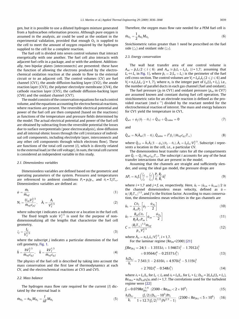
The net heat transfer rates are ~Q2 ¼ �~Q12 þ ~Qw2 þ ~Q23 þ ~Q2ohm,where ~Q23 ¼ ~ks;að1� /2Þ~Asðh2 � h3Þ=½ðn2 þ n3Þ=2�, where dual-poros-ity electrodes have been considered, as shown in Fig. 2.

The pores are approximated as parallel tubes with an averagediameter of the same order as the square root of the porous med-ium permeabilitiy, K1/2. Therefore, the wetted area for each porouscontrol volume is Aj;wet ¼ 4/jLjK

�1=2j As where Kj is the permeability.

The flow in the electrodes is modeled as Knudsen flow [23]. Thefuel and oxidant mass fluxes are given by

ji ¼ �½Dðqout � qinÞ=L�i ð17Þ

where D ¼ Bfr½8�RT=pM�1=2/qg, is the Knudsen diffusion coefficient,[24,25]. Therefore

Pi;out ¼ Pi;in �jiRkT1Lihi

Dip1; i ¼ 2;6; k ¼ f ; ox ð18Þ

where j2 ¼ _mH2=A3;wet and j6 ¼ _mo2=A5;wet , and A3;wet and A5;wet .The average pressures in CV2 and CV6 are estimated as

Pi ¼12ðPi;in � Pi;outÞ; i ¼ 2;6 ð19Þ

The energy balance delivers the CV2 temperature,

ðh1 � h2Þ þ~Q 2

wH2

¼ 0 ð20Þ

In the anode reaction layer (CV3), the electrical current is generatedby the electrochemical reaction,

H2ðgÞ ! 2HþðaqÞ þ 2e� ð21Þ

The dimensionless enthalpy of formation is defined by~Hi ¼ _niHi=ð _mref cp;f T1Þ, where the subscript i refers to a substanceor a control volume. The enthalpy change due to the anode reactionis given by DH3 ¼

Pproducts½tiHiðTiÞ� �

Preactants½tiHiðTiÞ� and We3 ¼

�DG3.The reaction Gibbs free energy change, DG, is a function of tem-

perature, pressure and concentrations, [26]

DG ¼ DG0 þ �RT ln Q ð22Þ

where DG0 = DH + TDS. Therefore, in the present reaction [Eq. (21)]the resulting expression for Q3 is Q3 ¼ ½HþðaqÞ�

2=pH2

, where ½HþðaqÞ�2 is

CV2 CV4 Perfluorosulfoniacid membrane

φ2 φ3

H2

CV3

y2 y4

ξ3/ξx ξ2/ξx ξ4/ξx

Fig. 2. Cross-sectional detail of dual-porosit

the molar concentration of the acid solution, (mol l�1), andpH2¼ p2;out .

The dimensionless net heat transfer in CV3 is given by~Q3 ¼ �~Q23 þ ~Qw3 þ ~Q34 þ ~Q 3ohm. The heat transfer rate betweenCV3 and CV4 (the polymer electrolyte membrane) is dominatedby conduction, therefore ~Q34 ¼ �ð1� /3Þðh3 � h4Þ ~As2~ks;a

~kp=

ðn4~ks;a þ n3

~kpÞ.The mass and energy balances for CV3, together with the anode

reaction equation deliver the relations _nH2 ¼ _mH2=MH2 ; _nHþ ¼2 _nH2 ; _mHþ ¼ 2 _nH2 MHþ and

~Q3 � D~H3 þ D~G3 ¼ 0 ð23Þ

where, ðD~H3;D~G3Þ ¼ _nH2 ðDH3;DG3Þ=ð _mref cp;f T1Þ.In the cathode reaction layer (CV5), the following reaction occurs

12

O2ðgÞ þ 2e� þ 2HþðaqÞ ! H2OðlÞ ð24Þ

Considering the mass conservation [Eqs. (22) and (25)] in CV4, wehave 2 _nH2 ¼ _nHþ ;out ¼ _nHþ ;in ¼ 2 _nO2 . In conclusion, _nH2 ¼ _nO2 , where_nO2 ¼ 2 _mO2=MO2 . Accordingly, the required oxidant mass flow rateis _mO2 ¼ _mH2 MO2=ð2MH2 Þ. The dimensionless net heat transfer inCV4 is obtained from ~Q4 ¼ �~Q34 þ ~Qw4 þ ~Q45 þ ~Q4ohm and ~Q45 ¼�ð1� /5Þðh4 � h5Þ~As2~ks;c

~kp=ðn4~ks;c þ n5

~kpÞ. Next, the CV4 tempera-ture is obtained from

~Q4 � ~Hðh3ÞHþðaqÞ� ~Hðh4ÞHþðaqÞ

¼ 0 ð25Þ

The analysis in the cathode reaction layer (CV5) is analogous towhat we previously presented in the anode reaction layer (CV3)analysis. The CV5 dimensionless temperature is obtained by

~Q5 � D~H5 þ D~G5 ¼ 0 ð26Þ

where ðD~H5;D~G5Þ ¼ _nO2 ðDH5;DG5Þ=ð _mref cp;f T1Þ; _nHþ ;in ¼ 2 _nO2_nH2O;out

¼ _nO2 .Similarly, the dimensionless net heat transfer rate flowing in

CV5 is given by ~Q5 ¼ �~Q 45 þ ~Qw5 þ ~Q 56 þ ~Q5ohm, with ~Q 56 ¼�~ks;cð1� /6Þ~Asðh5 � h6Þ=½ðn5 þ n6Þ=2�.

The enthalpy change during cathode reaction is DH5 ¼Pproducts½tiHiðTiÞ� �

Preac tan ts½tiHiðTiÞ�, while We5 = �DG5. The CV5

reaction quotient is Q 5 ¼ ½HþðaqÞ�2=p1=2

O2

n o�1, where pO2

¼ p6;out .

c

φ5 φ6

CV5

O2

Ionomer within the catalyst layer

CV6

y6

ξ6/ξx ξ5/ξx

y electrodes and the internal structure.

L.S. Martins et al. / Applied Thermal Engineering 29 (2009) 3036–3048 3041

The mass balance for CV6 yields _mO2;out ¼ _mO2;in ¼ _mO2 and_nH2O ¼ _nH2O2;out ¼ _nH2O2;in

¼ _nO2 . The dimensionless net heat transferrate in CV6 results from ~Q 6 ¼ �~Q 56 þ ~Q w6 þ ~Q 67 þ ~Q 6ohm, with~Q 67 ¼ ~h7

~Asð1� /6Þð/7 � /7Þ; ~h7 ¼ h7V2=3T =ð _mref cp;f Þ. The dimension-

less temperature for CV6 is given by

~Q 6 þ wHO2

cp;ox

cp;fðh7 � h6Þ þ ~Hðh5ÞH2O � ~Hðh6ÞH2O ¼ 0 ð27Þ

The dimensionless net heat transfer rate in CV7 is ~Q7 ¼�~Q67 þ ~Qw7 þ ~Q7ohm. The balances for mass and energy in the oxi-dant channel (CV7), the assumptions of non-mixing flow, and theassumption that the space is filled mainly with dry oxygen, yield_mH2O ¼ _mH2O;in ¼ _mH2O;out ¼ _nO2 MH2O and

~Q 7 þ woxcp;ox

cp;fðhox � h7Þ þ ~Hðh6ÞH2O � ~Hðh7ÞH2O ¼ 0 ð28Þ

2.4. Electrochemical model

Based on the electrical conductivities and geometry of eachcompartment, the electrical resistances, b(X), are given by:

bi ¼ni

~AsV1=3T rið1� /iÞ

; i ¼ 1;2;6;7 ð29Þ

bi ¼ni

~AsV1=3T ri/i

; i ¼ 3;4;5; ð/4 ¼ 1Þ ð30Þ

where the ionic conductivity, r(X�1 m�1), of Nafion 117 as afunc-tion of temperature is given by the following empirical formula[27]:

riðhÞ ¼ exp 12681

303� 1

hiT1

� �� �ð0:5139ki � 0:326Þ; i ¼ 3;4;5

ð31Þ

The conductivities of the catalyst layers are given by r3/3 and r5/5,according to Eqs. (30) and (31), which agree qualitatively with pre-viously measured catalyst layers ionic conductivities [28]. The con-ductivities of the diffusive layer, r2 and r6, are the carbon-phaseconductivities [29]. Finally, the conductivities of CV1 and CV7, r1

and r7, are given by the electrical conductivity of the bipolar platematerial.

Usually, the anode water content in the anode is different fromthe cathode [30]; therefore for assumed values of ka (anode watercontent) and kc (cathode water content), and by assuming a linearvariation of the water content along the membrane thickness, theaverage water content in the membrane s defined as

k ¼ ka þ kc

2ð32Þ

Eq. (32) allows for the calculation of ½HþðaqÞ� as a function of k, namely½HþðaqÞ� ffi qH2O=ðkMH2OÞ for a dilute water solution.

The appropriate figure of merit for evaluating the performanceof a fuel cell is the polarization curve, i.e., the fuel cell total poten-tial as a function of current. The dimensionless potential is definedin terms of a given reference voltage, Vref, namely ~V ¼ V=Vref and~g ¼ g=Vref . The dimensionless actual potential ~Vi is an accumulatedresult of dimensionless irreversible anode electrical potential ~Vi;a,dimensionless irreversible cathode electrical potential ~Vi;c , andthe dimensionless ohmic loss ð~gohmÞ in the space from CV1 toCV7, i.e.,

~Vi ¼ ~Ve;a þ ~Vi;c � ~gohm ð33Þ

The ohmic loss ~gohm is estimated by

~gohm ¼I

Vref

X7

i¼1

bi ð34Þ

The reversible electrical potential at the anode is given by theNernst equation [26],

Ve;a ¼ Voe;a �

�RT3

nFln Q 3 ð35Þ

where Ve;a ¼ DG3=ð�nFÞ and Voe;a ¼ DGo

3=ð�nFÞ. At the anode thereare two mechanisms for potential losses; (i) charge transfer, and(ii) mass diffusion. The potential loss (ga) due to charge transfer isobtained implicitly from the Butler–Volmer equation for a givencurrent I [30,31]

IA3;wet

¼ io;a expð1� aaÞgaF

�RT3

� �� exp �aagaF

�RT3

� �� �ð36Þ

The potential loss due to mass diffusion is [31,32]

gd;a ¼�RT3

nFln 1� I

A3;wetiLim;a

� �ð37Þ

where, from Eq. (18):

ilim;a ¼pf D2nF

MH2 L2Rf h2T1ð38Þ

The resulting electrical potential at the anode is ~Vi;a ¼~Ve;a � ~ga � j~gd;aj.

The methodology in estimating the anode potential is valid inbuilding the cathode potential correlations. Similarly, the actualcathode potential is ~Vi;c ¼ ~Ve;c � ~gc � j~gd;cj and the reversible elec-trical cathode potential is Ve;c ¼ Vo

e;c � ð�RT5=nFÞ ln Q5, whereQ5 ¼ ½HþðaqÞ�

2=p1=2

O2

n o�1and Vo

e;c ¼ DGo5=ð�nFÞ. The Butler–Volmer

equation for calculating the cathode side overpotential gc isI=A5;wet ¼ io;c½expðð1� acÞgcF=ð�RT5ÞÞ � expðacgcF=ð�RT5ÞÞ�. The cath-ode mass diffusion depleting overpotential isgd;c ¼ �RT5=ðnFÞ lnð1� I=ðA5;wetiLim;cÞÞ, and the cathode limiting cur-rent density is ilim;c ¼ 2poxD6nF=ðMO2 L6Roxh6T1Þ.

2.5. Fuel cell net power output

The pumping power ~Wp is required to supply the fuel cell withfuel and oxidant. Therefore the total net power (available for utili-zation) of the fuel cell is~Wnet ¼ ~W � ~Wp ð39Þ

where ~W ¼ ~Vi~I is the total fuel cell electrical power output, and

~Wp ¼ wf Sfhi

PiDP1 þ woxSox

h7

P7DP7 ð40Þ

Sf ¼mref T1Ri

Vref Iref; i ¼ f ; ox ð41Þ

3. Experiments

3.1. Experimental setup

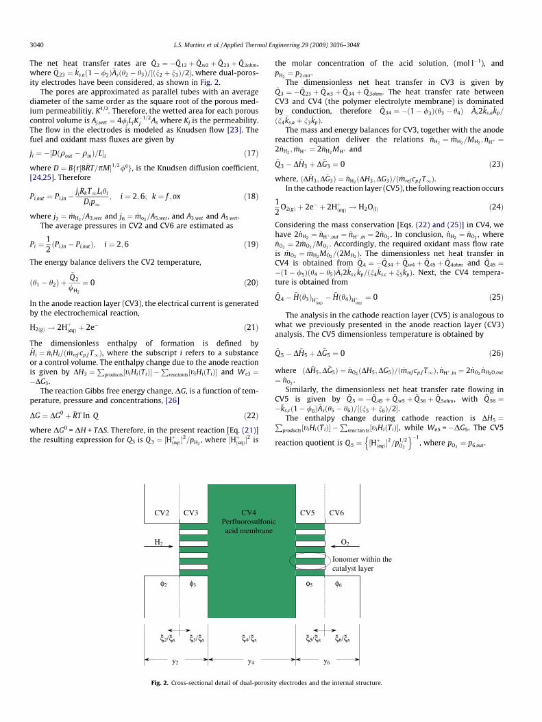
An experimental rig was built in the laboratory to produce thenecessary experimental data to perform the experimental valida-tion of the numerical results obtained with the mathematical mod-el presented in Section 2. Fig. 3 shows two photos of theexperimental set of single PEMFC’s utilized in this study. Ten lowpower (1–2 W) single PEMFC’s manufactured by Schatz Energy Re-search Center, SERC [33] were assembled on equally spaced sup-ports, as shown in Fig. 3a. On the lower right side of Fig. 3a, it isshown the dental oil free air compressor utilized to feed the sys-tem. The H2 and air feed systems with respective manometerswere placed on the wall, and from them a system of hoses andvalves distribute the fuel and oxidant supply to the cells. An adjust-able low power electric load was built with nickel-chrome alloywire, as shown in Fig. 3b.

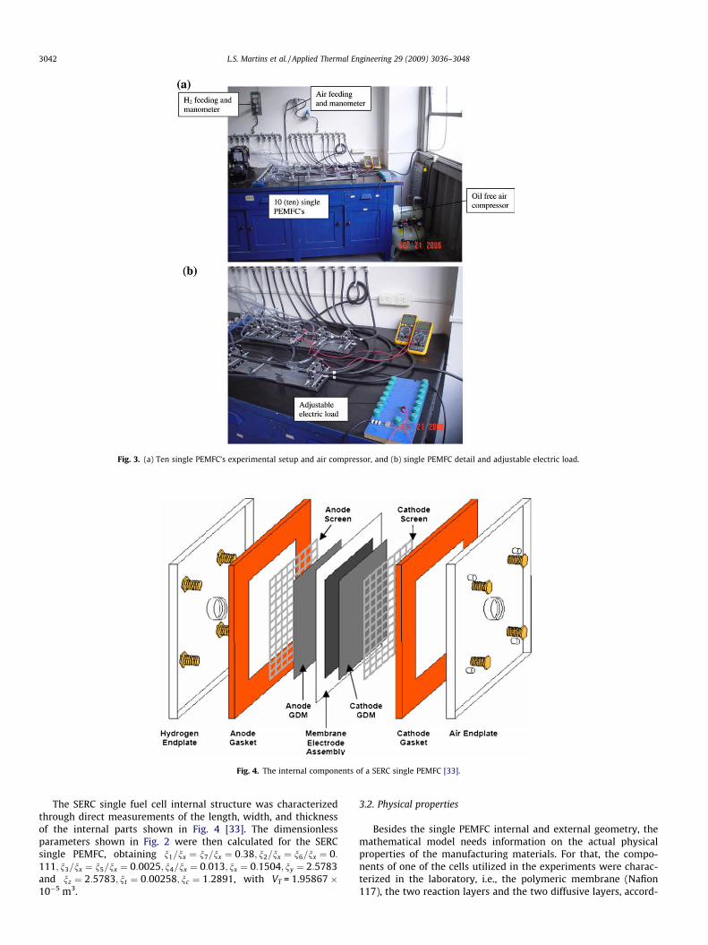
Fig. 3. (a) Ten single PEMFC’s experimental setup and air compressor, and (b) single PEMFC detail and adjustable electric load.

Fig. 4. The internal components of a SERC single PEMFC [33].

3042 L.S. Martins et al. / Applied Thermal Engineering 29 (2009) 3036–3048

The SERC single fuel cell internal structure was characterizedthrough direct measurements of the length, width, and thicknessof the internal parts shown in Fig. 4 [33]. The dimensionlessparameters shown in Fig. 2 were then calculated for the SERCsingle PEMFC, obtaining n1=nx ¼ n7=nx ¼ 0:38; n2=nx ¼ n6=nx ¼ 0:111; n3=nx ¼ n5=nx ¼ 0:0025; n4=nx ¼ 0:013; nx ¼ 0:1504; ny ¼ 2:5783and nz ¼ 2:5783; nt ¼ 0:00258; nc ¼ 1:2891, with VT = 1.95867 �10�5 m3.

3.2. Physical properties

Besides the single PEMFC internal and external geometry, themathematical model needs information on the actual physicalproperties of the manufacturing materials. For that, the compo-nents of one of the cells utilized in the experiments were charac-terized in the laboratory, i.e., the polymeric membrane (Nafion117), the two reaction layers and the two diffusive layers, accord-

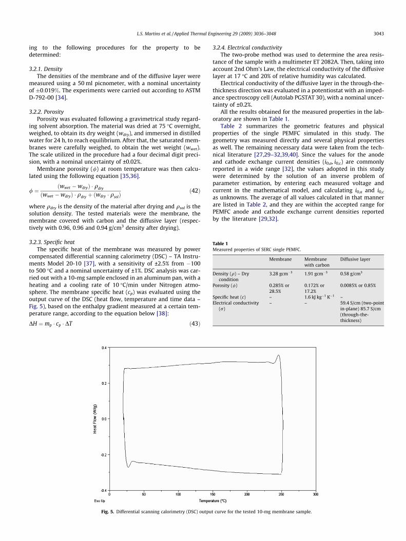
Table 1Measured properties of SERC single PEMFC.

Membrane Membranewith carbon

Diffusive layer

Density (q) – Drycondition

3.28 gcm�3 1.91 gcm�3 0.58 g/cm3

Porosity (/) 0.285% or28.5%

0.172% or17.2%

0.0085% or 0.85%

Specific heat (c) – 1.6 kJ kg�1 K�1 –Electrical conductivity

(r)– – 59.4 S/cm (two-point

in-plane) 85.7 S/cm(through-the-thickness)

L.S. Martins et al. / Applied Thermal Engineering 29 (2009) 3036–3048 3043

ing to the following procedures for the property to bedetermined:

3.2.1. DensityThe densities of the membrane and of the diffusive layer were

measured using a 50 ml picnometer, with a nominal uncertaintyof 0:019%. The experiments were carried out according to ASTMD-792-00 [34].

3.2.2. PorosityPorosity was evaluated following a gravimetrical study regard-

ing solvent absorption. The material was dried at 75 �C overnight,weighed, to obtain its dry weight (wdry), and immersed in distilledwater for 24 h, to reach equilibrium. After that, the saturated mem-branes were carefully weighed, to obtain the wet weight (wwet).The scale utilized in the procedure had a four decimal digit preci-sion, with a nominal uncertainty of ±0.02%.

Membrane porosity (/) at room temperature was then calcu-lated using the following equation [35,36].

/ ¼ðwwet �wdryÞ � qdry

ðwwet �wdryÞ � qdry þ ðwdry � qsolÞð42Þ

where qdry is the density of the material after drying and qsol is thesolution density. The tested materials were the membrane, themembrane covered with carbon and the diffusive layer (respec-tively with 0.96, 0.96 and 0.94 g/cm3 density after drying).

3.2.3. Specific heatThe specific heat of the membrane was measured by power

compensated differential scanning calorimetry (DSC) – TA Instru-ments Model 20-10 [37], with a sensitivity of ±2.5% from �100to 500 �C and a nominal uncertainty of ±1%. DSC analysis was car-ried out with a 10-mg sample enclosed in an aluminum pan, with aheating and a cooling rate of 10 �C/min under Nitrogen atmo-sphere. The membrane specific heat (cp) was evaluated using theoutput curve of the DSC (heat flow, temperature and time data –Fig. 5), based on the enthalpy gradient measured at a certain tem-perature range, according to the equation below [38]:

DH ¼ mp � cp � DT ð43Þ

Fig. 5. Differential scanning calorimetry (DSC) outpu

3.2.4. Electrical conductivityThe two-probe method was used to determine the area resis-

tance of the sample with a multimeter ET 2082A. Then, taking intoaccount 2nd Ohm’s Law, the electrical conductivity of the diffusivelayer at 17 �C and 20% of relative humidity was calculated.

Electrical conductivity of the diffusive layer in the through-the-thickness direction was evaluated in a potentiostat with an imped-ance spectroscopy cell (Autolab PGSTAT 30), with a nominal uncer-tainty of ±0.2%.

All the results obtained for the measured properties in the lab-oratory are shown in Table 1.

Table 2 summarizes the geometric features and physicalproperties of the single PEMFC simulated in this study. Thegeometry was measured directly and several physical propertiesas well. The remaining necessary data were taken from the tech-nical literature [27,29–32,39,40]. Since the values for the anodeand cathode exchange current densities (i0,a, i0,c) are commonlyreported in a wide range [32], the values adopted in this studywere determined by the solution of an inverse problem ofparameter estimation, by entering each measured voltage andcurrent in the mathematical model, and calculating i0,a and i0,c

as unknowns. The average of all values calculated in that mannerare listed in Table 2, and they are within the accepted range forPEMFC anode and cathode exchange current densities reportedby the literature [29,32].

t curve for the tested 10-mg membrane sample.

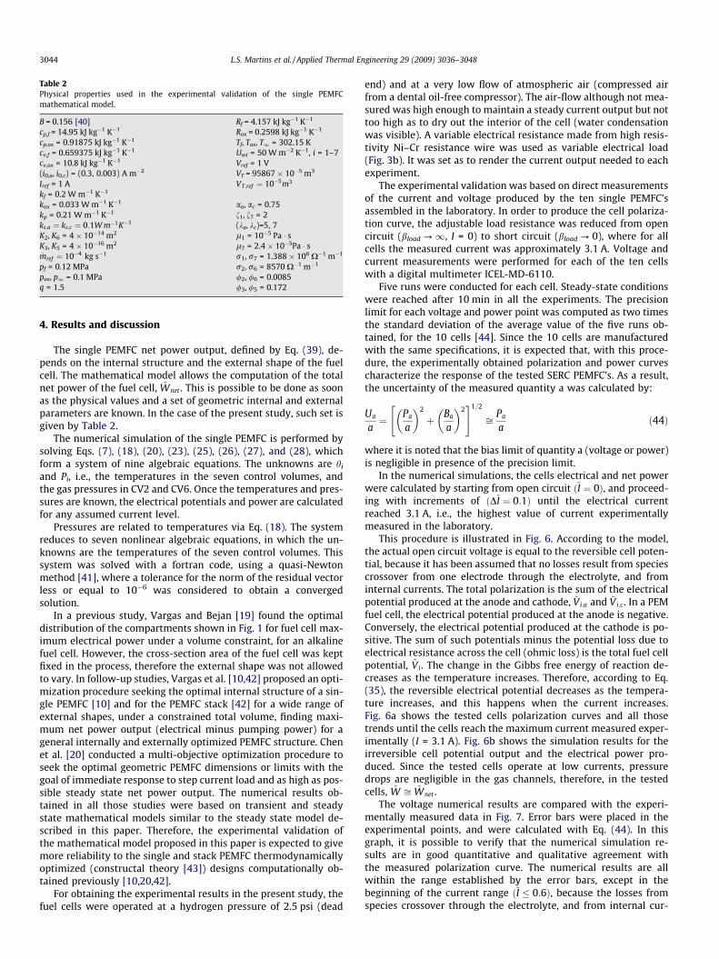
Table 2Physical properties used in the experimental validation of the single PEMFCmathematical model.

B = 0.156 [40] Rf = 4.157 kJ kg�1 K�1

cp,f = 14.95 kJ kg�1 K�1 Rox = 0.2598 kJ kg�1 K�1

cp,ox = 0.91875 kJ kg�1 K�1 Tf, Tox, T1 = 302.15 Kcv,f = 0.659375 kJ kg�1 K�1 Uwi = 50 W m�2 K�1, i = 1–7cv,ox = 10.8 kJ kg�1 K�1 Vref = 1 V(i0,a, i0,c) = (0.3, 0.003) A m�2 VT = 95867 � 10�5 m3

Iref = 1 A VT;ref ¼ 10�5m3

kf = 0.2 W m�1 K�1

kox = 0.033 W m�1 K�1 aa, ac = 0.75kp = 0.21 W m�1 K�1 f1, f7 = 2ks;a ¼ ks;c ¼ 0:1W m�1K�1 (ka, kc)=5, 7K2, K6 = 4 � 10�14 m2 l1 = 10�5 Pa � sK3, K5 = 4 � 10�16 m2 l7 = 2.4 � 10�5Pa � s_mref ¼ 10�4 kg s�1 r1, r7 = 1.388 � 106 X�1 m�1

pf = 0.12 MPa r2, r6 = 8570 X�1 m�1

pox, p1 = 0.1 MPa /2, /6 = 0.0085q = 1.5 /3, /5 = 0.172

3044 L.S. Martins et al. / Applied Thermal Engineering 29 (2009) 3036–3048

4. Results and discussion

The single PEMFC net power output, defined by Eq. (39), de-pends on the internal structure and the external shape of the fuelcell. The mathematical model allows the computation of the totalnet power of the fuel cell, ~Wnet . This is possible to be done as soonas the physical values and a set of geometric internal and externalparameters are known. In the case of the present study, such set isgiven by Table 2.

The numerical simulation of the single PEMFC is performed bysolving Eqs. (7), (18), (20), (23), (25), (26), (27), and (28), whichform a system of nine algebraic equations. The unknowns are hi

and Pi, i.e., the temperatures in the seven control volumes, andthe gas pressures in CV2 and CV6. Once the temperatures and pres-sures are known, the electrical potentials and power are calculatedfor any assumed current level.

Pressures are related to temperatures via Eq. (18). The systemreduces to seven nonlinear algebraic equations, in which the un-knowns are the temperatures of the seven control volumes. Thissystem was solved with a fortran code, using a quasi-Newtonmethod [41], where a tolerance for the norm of the residual vectorless or equal to 10�6 was considered to obtain a convergedsolution.

In a previous study, Vargas and Bejan [19] found the optimaldistribution of the compartments shown in Fig. 1 for fuel cell max-imum electrical power under a volume constraint, for an alkalinefuel cell. However, the cross-section area of the fuel cell was keptfixed in the process, therefore the external shape was not allowedto vary. In follow-up studies, Vargas et al. [10,42] proposed an opti-mization procedure seeking the optimal internal structure of a sin-gle PEMFC [10] and for the PEMFC stack [42] for a wide range ofexternal shapes, under a constrained total volume, finding maxi-mum net power output (electrical minus pumping power) for ageneral internally and externally optimized PEMFC structure. Chenet al. [20] conducted a multi-objective optimization procedure toseek the optimal geometric PEMFC dimensions or limits with thegoal of immediate response to step current load and as high as pos-sible steady state net power output. The numerical results ob-tained in all those studies were based on transient and steadystate mathematical models similar to the steady state model de-scribed in this paper. Therefore, the experimental validation ofthe mathematical model proposed in this paper is expected to givemore reliability to the single and stack PEMFC thermodynamicallyoptimized (constructal theory [43]) designs computationally ob-tained previously [10,20,42].

For obtaining the experimental results in the present study, thefuel cells were operated at a hydrogen pressure of 2.5 psi (dead

end) and at a very low flow of atmospheric air (compressed airfrom a dental oil-free compressor). The air-flow although not mea-sured was high enough to maintain a steady current output but nottoo high as to dry out the interior of the cell (water condensationwas visible). A variable electrical resistance made from high resis-tivity Ni–Cr resistance wire was used as variable electrical load(Fig. 3b). It was set as to render the current output needed to eachexperiment.

The experimental validation was based on direct measurementsof the current and voltage produced by the ten single PEMFC’sassembled in the laboratory. In order to produce the cell polariza-tion curve, the adjustable load resistance was reduced from opencircuit (bload ?1, I = 0) to short circuit (bload ? 0), where for allcells the measured current was approximately 3.1 A. Voltage andcurrent measurements were performed for each of the ten cellswith a digital multimeter ICEL-MD-6110.

Five runs were conducted for each cell. Steady-state conditionswere reached after 10 min in all the experiments. The precisionlimit for each voltage and power point was computed as two timesthe standard deviation of the average value of the five runs ob-tained, for the 10 cells [44]. Since the 10 cells are manufacturedwith the same specifications, it is expected that, with this proce-dure, the experimentally obtained polarization and power curvescharacterize the response of the tested SERC PEMFC’s. As a result,the uncertainty of the measured quantity a was calculated by:

Ua

a¼ Pa

a

� �2

þ Ba

a

� �2" #1=2

ffi Pa

að44Þ

where it is noted that the bias limit of quantity a (voltage or power)is negligible in presence of the precision limit.

In the numerical simulations, the cells electrical and net powerwere calculated by starting from open circuit ð~I ¼ 0Þ, and proceed-ing with increments of ðD~I ¼ 0:1Þ until the electrical currentreached 3.1 A, i.e., the highest value of current experimentallymeasured in the laboratory.

This procedure is illustrated in Fig. 6. According to the model,the actual open circuit voltage is equal to the reversible cell poten-tial, because it has been assumed that no losses result from speciescrossover from one electrode through the electrolyte, and frominternal currents. The total polarization is the sum of the electricalpotential produced at the anode and cathode, ~Vi;a and ~Vi;c. In a PEMfuel cell, the electrical potential produced at the anode is negative.Conversely, the electrical potential produced at the cathode is po-sitive. The sum of such potentials minus the potential loss due toelectrical resistance across the cell (ohmic loss) is the total fuel cellpotential, ~Vi. The change in the Gibbs free energy of reaction de-creases as the temperature increases. Therefore, according to Eq.(35), the reversible electrical potential decreases as the tempera-ture increases, and this happens when the current increases.Fig. 6a shows the tested cells polarization curves and all thosetrends until the cells reach the maximum current measured exper-imentally (I = 3.1 A). Fig. 6b shows the simulation results for theirreversible cell potential output and the electrical power pro-duced. Since the tested cells operate at low currents, pressuredrops are negligible in the gas channels, therefore, in the testedcells, ~W ffi ~Wnet .

The voltage numerical results are compared with the experi-mentally measured data in Fig. 7. Error bars were placed in theexperimental points, and were calculated with Eq. (44). In thisgraph, it is possible to verify that the numerical simulation re-sults are in good quantitative and qualitative agreement withthe measured polarization curve. The numerical results are allwithin the range established by the error bars, except in thebeginning of the current range ð~I � 0:6Þ, because the losses fromspecies crossover through the electrolyte, and from internal cur-

-0.5

0

0.5

1

1.5

0 0.5 1 1.5 2 2.5 3 3.5

eV~

iV~

ci,V~

ai,ci, V~

,V~

ie V~

,V~

I~

ai,V~

(a)

0.5

0.6

0.7

0.8

0.9

1

1.1

1.2

0

0.5

1

1.5

2

0 0.5 1 1.5 2 2.5 3

I~

W~

W~

iV~

iV~

(b)

Fig. 6. (a) Total cell reversible, cathode, total cell irreversible, and anode numerically simulated potentials from top to bottom, and (b) the numerically simulated total cellirreversible potential and output power.

0.4

0.6

0.8

1

1.2

1.4

0 0.4 0.8 1.2 1.6 2 2.4 2.8 3.2

experimental

I~

numericaliV~

Fig. 7. The comparison between the numerically and experimentally obtained totalcell irreversible potential.

L.S. Martins et al. / Applied Thermal Engineering 29 (2009) 3036–3048 3045

rents are not considered in the mathematical model. However, inpractice, fuel cells are expected to operate at higher currents,where maximum power occurs, therefore the model is expected

to provide output voltage accurate results at that current rangeof greater interest.

Fig. 8 depicts the comparison of the cells output power betweenthe obtained numerical and experimental results. It is observedthat the numerical simulation results fall within the range estab-lished by the error bars in the entire current range analyzed inthe experiments ð0 6 I 6 3:1 AÞ. This shows good quantitativeand qualitative agreement between numerical and experimentalresults. Therefore, the model is expected to provide output poweraccurate results in the entire PEMFC current range of operation.

Next, the variation of PEMFC temperature with respect to spaceand operating current is addressed. It is a common practice in thetechnical literature to assume uniform operating temperaturethroughout the single PEMFC or PEMFC stack, operating in the en-tire current range of the cell. The following experimental observa-tions intend to show the importance of considering temperaturedependence on space and current in PEMFC mathematical models.The mathematical model validated in this paper shows that tem-perature variations inside the cell could change substantially cellvoltage and power output, since all calculated potentials dependon local temperature at a particular location in the PEMFC accord-ing to Fig. 1. To achieve this goal, noninvasive surface temperaturemeasurements were utilized, with an infrared camera.

The infrared images were obtained using a SAT-S160 Infraredcamera from the Guagzhou SAR Infrared Technology Co. (China).

0

0.45

0.9

1.35

1.8

0 0.5 1 1.5 2 2.5 3 3.5

experimentalnumerical

I~

W~

Fig. 8. The comparison between the numerically and experimentally obtained totalcell output power.

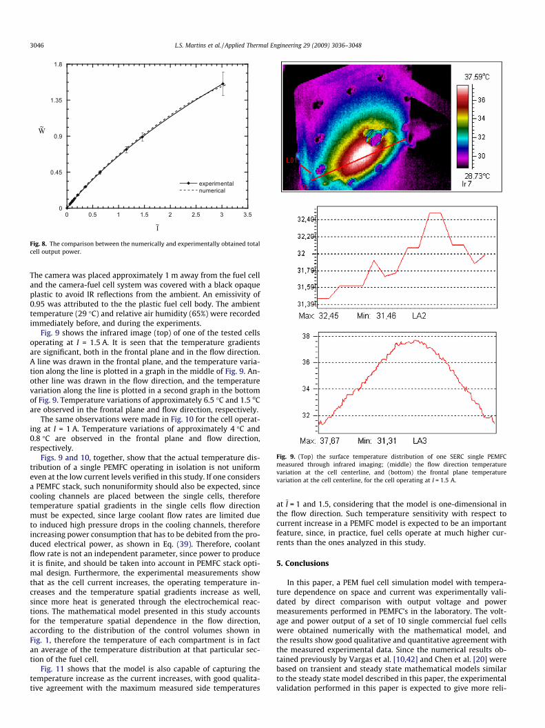
Fig. 9. (Top) the surface temperature distribution of one SERC single PEMFCmeasured through infrared imaging; (middle) the flow direction temperaturevariation at the cell centerline, and (bottom) the frontal plane temperaturevariation at the cell centerline, for the cell operating at I = 1.5 A.

3046 L.S. Martins et al. / Applied Thermal Engineering 29 (2009) 3036–3048

The camera was placed approximately 1 m away from the fuel celland the camera-fuel cell system was covered with a black opaqueplastic to avoid IR reflections from the ambient. An emissivity of0.95 was attributed to the the plastic fuel cell body. The ambienttemperature (29 �C) and relative air humidity (65%) were recordedimmediately before, and during the experiments.

Fig. 9 shows the infrared image (top) of one of the tested cellsoperating at I = 1.5 A. It is seen that the temperature gradientsare significant, both in the frontal plane and in the flow direction.A line was drawn in the frontal plane, and the temperature varia-tion along the line is plotted in a graph in the middle of Fig. 9. An-other line was drawn in the flow direction, and the temperaturevariation along the line is plotted in a second graph in the bottomof Fig. 9. Temperature variations of approximately 6.5 �C and 1.5 oCare observed in the frontal plane and flow direction, respectively.

The same observations were made in Fig. 10 for the cell operat-ing at I = 1 A. Temperature variations of approximately 4 �C and0.8 �C are observed in the frontal plane and flow direction,respectively.

Figs. 9 and 10, together, show that the actual temperature dis-tribution of a single PEMFC operating in isolation is not uniformeven at the low current levels verified in this study. If one considersa PEMFC stack, such nonuniformity should also be expected, sincecooling channels are placed between the single cells, thereforetemperature spatial gradients in the single cells flow directionmust be expected, since large coolant flow rates are limited dueto induced high pressure drops in the cooling channels, thereforeincreasing power consumption that has to be debited from the pro-duced electrical power, as shown in Eq. (39). Therefore, coolantflow rate is not an independent parameter, since power to produceit is finite, and should be taken into account in PEMFC stack opti-mal design. Furthermore, the experimental measurements showthat as the cell current increases, the operating temperature in-creases and the temperature spatial gradients increase as well,since more heat is generated through the electrochemical reac-tions. The mathematical model presented in this study accountsfor the temperature spatial dependence in the flow direction,according to the distribution of the control volumes shown inFig. 1, therefore the temperature of each compartment is in factan average of the temperature distribution at that particular sec-tion of the fuel cell.

Fig. 11 shows that the model is also capable of capturing thetemperature increase as the current increases, with good qualita-tive agreement with the maximum measured side temperatures

at ~I = 1 and 1.5, considering that the model is one-dimensional inthe flow direction. Such temperature sensitivity with respect tocurrent increase in a PEMFC model is expected to be an importantfeature, since, in practice, fuel cells operate at much higher cur-rents than the ones analyzed in this study.

5. Conclusions

In this paper, a PEM fuel cell simulation model with tempera-ture dependence on space and current was experimentally vali-dated by direct comparison with output voltage and powermeasurements performed in PEMFC’s in the laboratory. The volt-age and power output of a set of 10 single commercial fuel cellswere obtained numerically with the mathematical model, andthe results show good qualitative and quantitative agreement withthe measured experimental data. Since the numerical results ob-tained previously by Vargas et al. [10,42] and Chen et al. [20] werebased on transient and steady state mathematical models similarto the steady state model described in this paper, the experimentalvalidation performed in this paper is expected to give more reli-

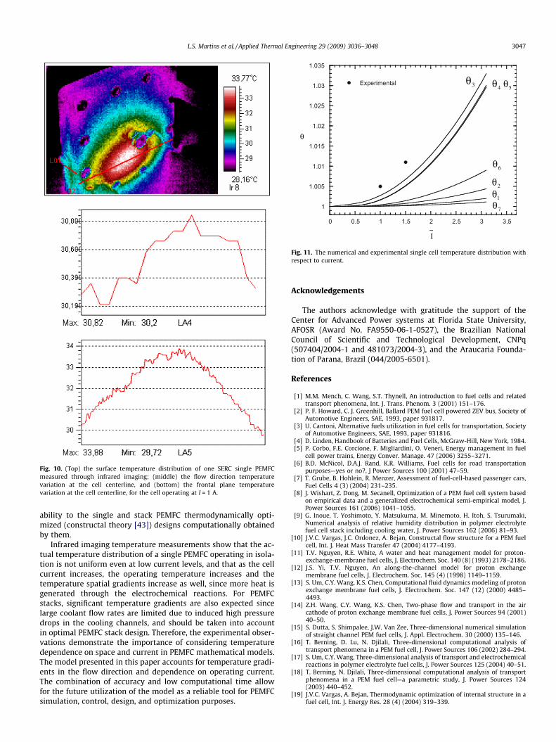
Fig. 10. (Top) the surface temperature distribution of one SERC single PEMFCmeasured through infrared imaging; (middle) the flow direction temperaturevariation at the cell centerline, and (bottom) the frontal plane temperaturevariation at the cell centerline, for the cell operating at I = 1 A.

1

1.005

1.01

1.015

1.02

1.025

1.03

1.035

0 0.5 1 1.5 2 2.5 3 3.5

Experimental

I~

θ

7θ

6θ

5θ4θ3θ

2θ1θ

Fig. 11. The numerical and experimental single cell temperature distribution withrespect to current.

L.S. Martins et al. / Applied Thermal Engineering 29 (2009) 3036–3048 3047

ability to the single and stack PEMFC thermodynamically opti-mized (constructal theory [43]) designs computationally obtainedby them.

Infrared imaging temperature measurements show that the ac-tual temperature distribution of a single PEMFC operating in isola-tion is not uniform even at low current levels, and that as the cellcurrent increases, the operating temperature increases and thetemperature spatial gradients increase as well, since more heat isgenerated through the electrochemical reactions. For PEMFCstacks, significant temperature gradients are also expected sincelarge coolant flow rates are limited due to induced high pressuredrops in the cooling channels, and should be taken into accountin optimal PEMFC stack design. Therefore, the experimental obser-vations demonstrate the importance of considering temperaturedependence on space and current in PEMFC mathematical models.The model presented in this paper accounts for temperature gradi-ents in the flow direction and dependence on operating current.The combination of accuracy and low computational time allowfor the future utilization of the model as a reliable tool for PEMFCsimulation, control, design, and optimization purposes.

Acknowledgements

The authors acknowledge with gratitude the support of theCenter for Advanced Power systems at Florida State University,AFOSR (Award No. FA9550-06-1-0527), the Brazilian NationalCouncil of Scientific and Technological Development, CNPq(507404/2004-1 and 481073/2004-3), and the Araucaria Founda-tion of Parana, Brazil (044/2005-6501).

References

[1] M.M. Mench, C. Wang, S.T. Thynell, An introduction to fuel cells and relatedtransport phenomena, Int. J. Trans. Phenom. 3 (2001) 151–176.

[2] P. F. Howard, C. J. Greenhill, Ballard PEM fuel cell powered ZEV bus, Society ofAutomotive Engineers, SAE, 1993, paper 931817.

[3] U. Cantoni, Alternative fuels utilization in fuel cells for transportation, Societyof Automotive Engineers, SAE, 1993, paper 931816.

[4] D. Linden, Handbook of Batteries and Fuel Cells, McGraw-Hill, New York, 1984.[5] P. Corbo, F.E. Corcione, F. Migliardini, O. Veneri, Energy management in fuel

cell power trains, Energy Conver. Manage. 47 (2006) 3255–3271.[6] B.D. McNicol, D.A.J. Rand, K.R. Williams, Fuel cells for road transportation

purposes—yes or no?, J Power Sources 100 (2001) 47–59.[7] T. Grube, B. Hohlein, R. Menzer, Assessment of fuel-cell-based passenger cars,

Fuel Cells 4 (3) (2004) 231–235.[8] J. Wishart, Z. Dong, M. Secanell, Optimization of a PEM fuel cell system based

on empirical data and a generalized electrochemical semi-empirical model, J.Power Sources 161 (2006) 1041–1055.

[9] G. Inoue, T. Yoshimoto, Y. Matsukuma, M. Minemoto, H. Itoh, S. Tsurumaki,Numerical analysis of relative humidity distribution in polymer electrolytefuel cell stack including cooling water, J. Power Sources 162 (2006) 81–93.

[10] J.V.C. Vargas, J.C. Ordonez, A. Bejan, Constructal flow structure for a PEM fuelcell, Int. J. Heat Mass Transfer 47 (2004) 4177–4193.

[11] T.V. Nguyen, R.E. White, A water and heat management model for proton-exchange-membrane fuel cells, J. Electrochem. Soc. 140 (8) (1993) 2178–2186.

[12] J.S. Yi, T.V. Nguyen, An along-the-channel model for proton exchangemembrane fuel cells, J. Electrochem. Soc. 145 (4) (1998) 1149–1159.

[13] S. Um, C.Y. Wang, K.S. Chen, Computational fluid dynamics modeling of protonexchange membrane fuel cells, J. Electrochem. Soc. 147 (12) (2000) 4485–4493.

[14] Z.H. Wang, C.Y. Wang, K.S. Chen, Two-phase flow and transport in the aircathode of proton exchange membrane fuel cells, J. Power Sources 94 (2001)40–50.

[15] S. Dutta, S. Shimpalee, J.W. Van Zee, Three-dimensional numerical simulationof straight channel PEM fuel cells, J. Appl. Electrochem. 30 (2000) 135–146.

[16] T. Berning, D. Lu, N. Djilali, Three-dimensional computational analysis oftransport phenomena in a PEM fuel cell, J. Power Sources 106 (2002) 284–294.

[17] S. Um, C.Y. Wang, Three-dimensional analysis of transport and electrochemicalreactions in polymer electrolyte fuel cells, J. Power Sources 125 (2004) 40–51.

[18] T. Berning, N. Djilali, Three-dimensional computational analysis of transportphenomena in a PEM fuel cell—a parametric study, J. Power Sources 124(2003) 440–452.

[19] J.V.C. Vargas, A. Bejan, Thermodynamic optimization of internal structure in afuel cell, Int. J. Energy Res. 28 (4) (2004) 319–339.

3048 L.S. Martins et al. / Applied Thermal Engineering 29 (2009) 3036–3048

[20] S. Chen, J.C. Ordonez, J.V.C. Vargas, J.E.F.C. Gardolinski, M.A.B. Gomes, Transientoperation and shape optimization of a single PEM fuel cell, J. Power Sources162 (2006) 356–368.

[21] R.K. Shah, A.L. London, in: Laminar Flow Forced Convection in Ducts,Supplement 1 to Advances in Heat Transfer, Academic Press, New York, 1978.

[22] A. Bejan, Convection Heat Transfer, second ed., Wiley, New York, 1995.[23] R.B. Bird, W.E. Stewart, E.N. Lightfoot, Transport Phenomena, second ed.,

Wiley, New York, 2002.[24] J.S. Newman, Electrochemical Systems, second ed., Prentice Hall, Englewood

Cliffs, NJ, 1991. pp. 255, 299, 461.[25] J.A. Wesselingh, P. Vonk, G. Kraaijeveld, Exploring the Maxwell–Stefan

description of ion-exchange, Chem. Eng. J. Biochem. Eng. J. 57 (1995) 75–89.

[26] W.L. Masterton, C.N. Hurley, Chemistry Principles and Reactions, third ed.,Saunders College Publishing, Orlando, FL, 1997.

[27] T.E. Springer, T.A. Zawodzinski, S. Gottesfeld, Polymer electrolyte fuel cellmodel, J. Electrochem. Soc. 138 (1991) 2334–2341.

[28] G. Li, P.G. Pickup, Ionic conductivity of PEMFC electrodes, J. Electrochem. Soc.150 (11) (2003) C745–C752.

[29] A.A. Kulikovsky, J. Divisek, A.A. Kornyshev, Two-dimensional simulation ofdirect methanol fuel cells –a new (embedded) type of current collector, J.Electrochem. Soc. (147) (2000) 953–959.

[30] V. Gurau, F. Barbir, H. Liu, An analytical solution of a half-cell model for PEMfuel cells, J. Electrochem. Soc. 147 (2000) 2468–2477.

[31] J.O’M. Bockris, D.M. Drazic, Electro-chemical Science, Taylor and Francis,London, 1972.

[32] A.J. Bard, L.R. Faulkner, Electrochemical Methods – Fundamentals andApplications, second ed., Wiley, New York, 2001.

[33] Schatz Energy Research Center, Operation and Maintainance Manual – SERCSingle Cell Fuel Cell Kit, Humboldt State University, Arcata, CA, USA, 2004.

[34] ASTM – D792-00 Standard Test Methods for Density and Specific Gravity(Relative Density) of Plastics by Displacement, ASTM International, 2000.

[35] D. Sangeetha, Conductivity and solvent uptake of proto exchange membranebased on polystyrene (ethylene–butylene) polystyrene triblock polymer, Eur.Polym. J. 41 (11) (2005) 2644–2652.

[36] Y. Elabd, E. Napadensky, Sulfonation and characterization of poly(styrene-isobutylene-styrene) triblock copolymers at high ion-exchange capacities,Polymer 45 (2004) 3037–3043.

[37] J. Morikawa, A. Kobayahi, T. Hashimoto, Thermal diffusivity in a binarymixture of poly (phenylene oxide) and polystyrene, Thermochim. Acta 267 (1)(2005) 289–296.

[38] C.M.A. Lopes, M.I. Felisberti, Thermal conductivity of PET/(LDOE/AI)composites determined by MDSC, Polym. Test. 23 (2004) 637–643.

[39] D.R. Lide (Ed.), CRC Handbook of Chemistry and Physics, Eight-third ed., CRCPress, Boca Raton, FL, 2002.

[40] M.R. Tarasevich, A. Sadkowski, E. Yeager, in: B.E. Coway, J.O’M. Bockris, E.Yeager, S.U.M. Khan, R.E. White (Eds.), Comprehensive Treatise ofElectrochemistry, vol. 7, Plenum, New York, 1983, pp. 310–398.

[41] D. Kincaid, W. Cheney, Numerical Analysis Mathematics of ScientificComputing, first ed., Wadsworth, Belmont, CA, 1991.

[42] J.V.C. Vargas, J.C. Ordonez, A. Bejan, Constructal PEM fuel cell stack design, Int.J. Heat Mass Transfer 48 (2005) 4410–4427.

[43] A. Bejan, Shape and Structure, from Engineering to Nature, CambridgeUniversity Press, Cambridge, UK, 2000.

[44] Editorial, Journal of Heat Transfer policy on reporting uncertainties inexperimental measurements and results, ASME J. Heat Transfer, 115 (1993) 5–6.