Applied Quantitative Analysis and Practices

LECTURE#16

By

Dr. Osman Sadiq Paracha

Lecture Summary Assumptions in testing of hypothesis

Additivity and linearity Normality Homogeneity of Variance Independence

Reduction of Bias Trim the data: Windsorizing: Analyse with Robust Methods: Transform the data:

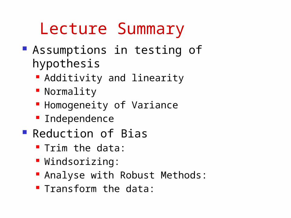
Transforming Data Log Transformation (log(Xi))

Reduce positive skew. Square Root Transformation (√Xi):

Also reduces positive skew. Can also be useful for stabilizing variance.

Reciprocal Transformation (1/ Xi): Dividing 1 by each score also reduces the impact of

large scores. This transformation reverses the scores, you can avoid this by reversing the scores before the transformation, 1/(XHighest – Xi).

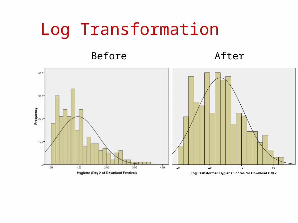
Log Transformation

Before After

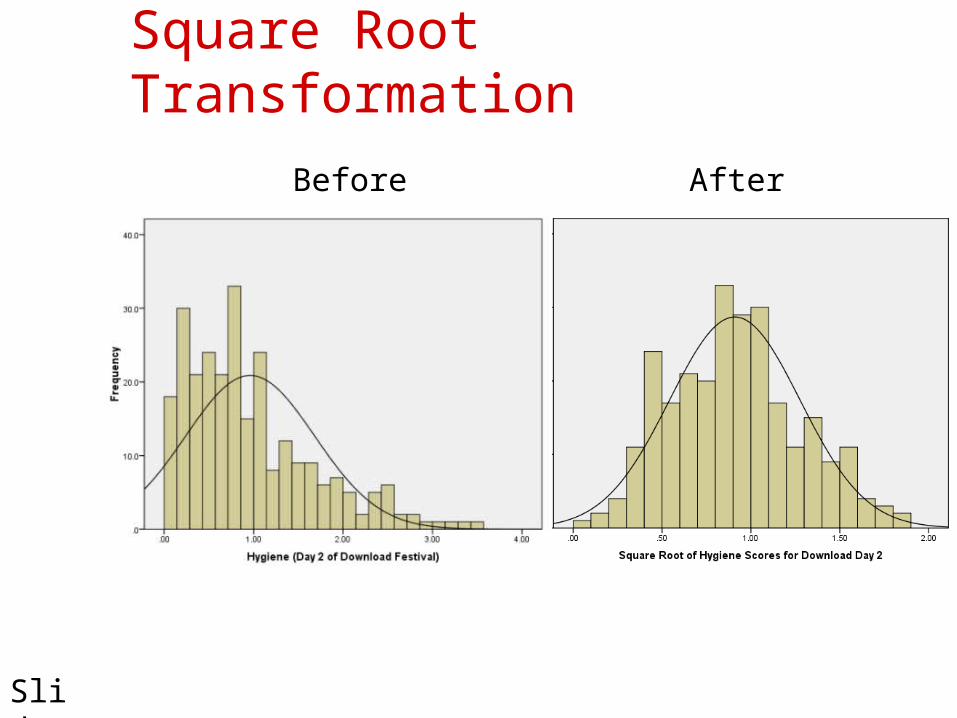
Square Root Transformation

Slide 5

Before After

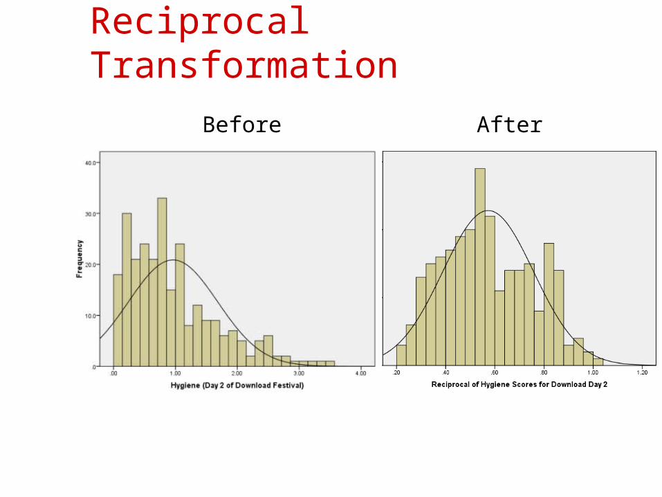
Reciprocal Transformation

Before After

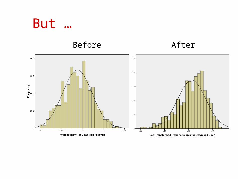
But …

Before After

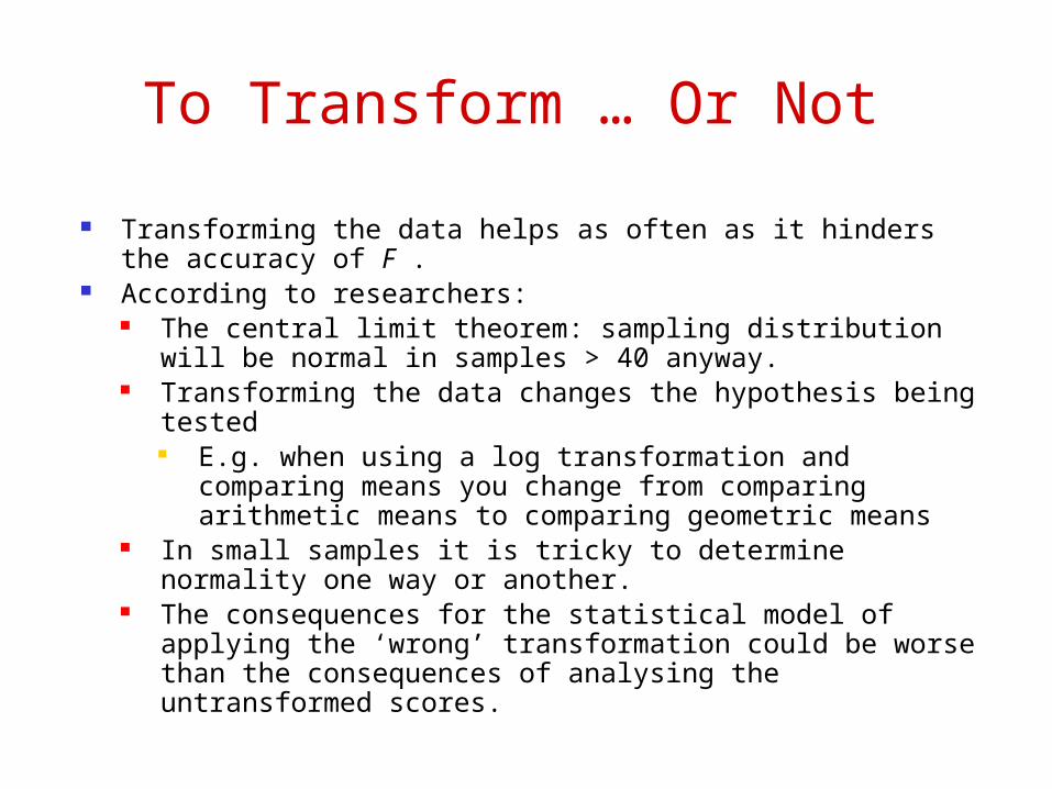
To Transform … Or Not

Transforming the data helps as often as it hinders the accuracy of F .

According to researchers: The central limit theorem: sampling distribution will be normal in

samples > 40 anyway. Transforming the data changes the hypothesis being tested

E.g. when using a log transformation and comparing means you change from comparing arithmetic means to comparing geometric means

In small samples it is tricky to determine normality one way or another.

The consequences for the statistical model of applying the ‘wrong’ transformation could be worse than the consequences of analysing the untransformed scores.

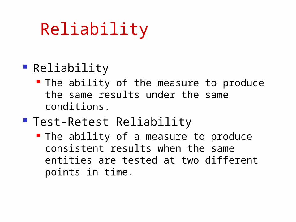
Reliability

Reliability The ability of the measure to produce the same

results under the same conditions. Test-Retest Reliability

The ability of a measure to produce consistent results when the same entities are tested at two different points in time.

Cronbach’s alphaassessing scale reliability

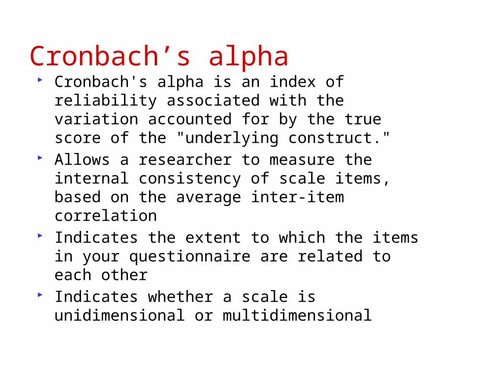
Cronbach’s alpha Cronbach's alpha is an index of reliability associated

with the variation accounted for by the true score of the "underlying construct."

Allows a researcher to measure the internal consistency of scale items, based on the average inter-item correlation

Indicates the extent to which the items in your questionnaire are related to each other

Indicates whether a scale is unidimensional or multidimensional

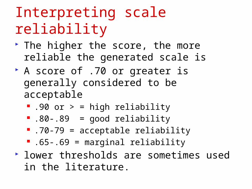
Interpreting scale reliability The higher the score, the more reliable the

generated scale is A score of .70 or greater is generally considered

to be acceptable .90 or > = high reliability .80-.89 = good reliability .70-79 = acceptable reliability .65-.69 = marginal reliability

lower thresholds are sometimes used in the literature.

Validity

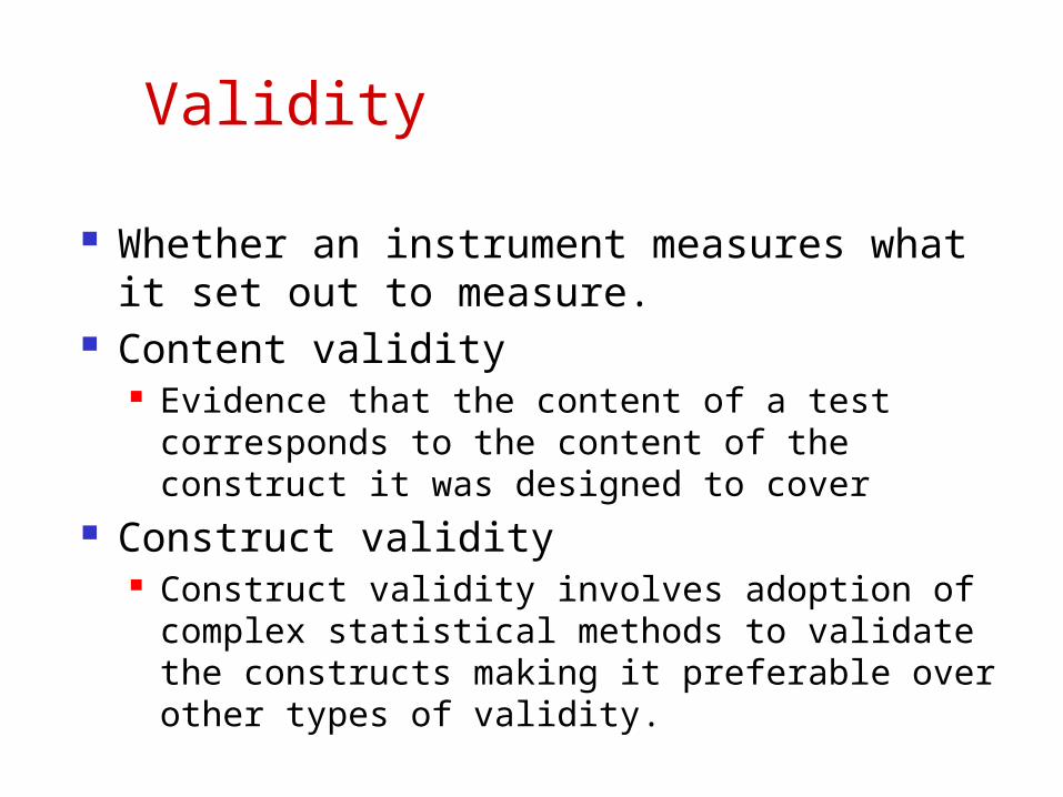
Whether an instrument measures what it set out to measure.

Content validity Evidence that the content of a test corresponds to

the content of the construct it was designed to cover Construct validity

Construct validity involves adoption of complex statistical methods to validate the constructs making it preferable over other types of validity.

Exploratory Factor Analysis

Exploratory factor analysis . . . is an

interdependence technique whose primary

purpose is to define the underlying structure

among the variables in the analysis.

Exploratory Factor Analysis Defined

Exploratory Factor Analysis . . .

• Examines the interrelationships among a large number of variables and then attempts to explain them in terms of their common underlying dimensions.

• These common underlying dimensions are referred to as factors.

• A summarization and data reduction technique that does not have independent and dependent variables, but is an interdependence technique in which all variables are considered simultaneously.

What is Exploratory Factor Analysis?

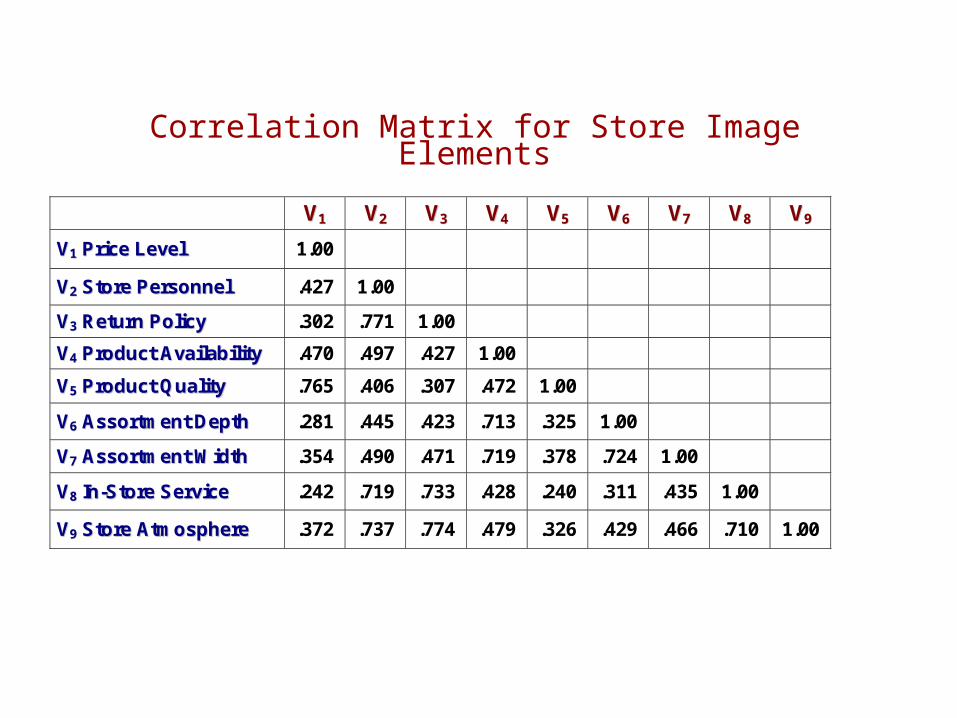
Correlation Matrix for Store Image Elements

VV11 VV22 VV33 VV44 VV55 VV66 VV77 VV88 VV99

VV11 PPrriiccee LLeevveell 1.00

VV22 SSttoorree PPeerrssoonnnneell .427 1.00

VV33 RReettuurrnn PPoolliiccyy .302 .771 1.00

VV44 PPrroodduucctt AAvvaaiillaabbiilliittyy .470 .497 .427 1.00

VV55 PPrroodduucctt QQuuaalliittyy .765 .406 .307 .472 1.00

VV66 AAssssoorrttmmeenntt DDeepptthh .281 .445 .423 .713 .325 1.00

VV77 AAssssoorrttmmeenntt WWiiddtthh .354 .490 .471 .719 .378 .724 1.00

VV88 IInn--SSttoorree SSeerrvviiccee .242 .719 .733 .428 .240 .311 .435 1.00

VV99 SSttoorree AAttmmoosspphheerree .372 .737 .774 .479 .326 .429 .466 .710 1.00

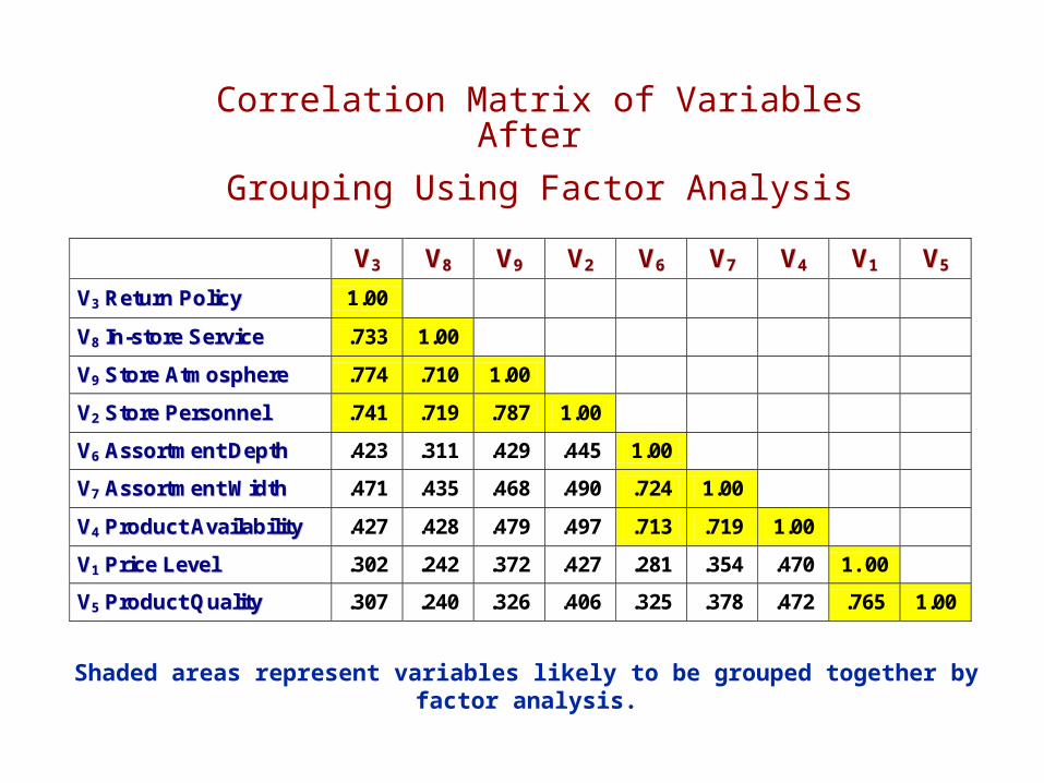
Correlation Matrix of Variables After

Grouping Using Factor Analysis

Shaded areas represent variables likely to be grouped together by factor analysis.

VV33 VV88 VV99 VV22 VV66 VV77 VV44 VV11 VV55

VV33 RReettuurrnn PPoolliiccyy 1.00

VV88 IInn--ssttoorree SSeerrvviiccee .733 1.00

VV99 SSttoorree AAttmmoosspphheerree .774 .710 1.00

VV22 SSttoorree PPeerrssoonnnneell .741 .719 .787 1.00

VV66 AAssssoorrttmmeenntt DDeepptthh .423 .311 .429 .445 1.00

VV77 AAssssoorrttmmeenntt WWiiddtthh .471 .435 .468 .490 .724 1.00

VV44 PPrroodduucctt AAvvaaiillaabbiilliittyy .427 .428 .479 .497 .713 .719 1.00

VV11 PPrriiccee LLeevveell .302 .242 .372 .427 .281 .354 .470 1. 00

VV55 PPrroodduucctt QQuuaalliittyy .307 .240 .326 .406 .325 .378 .472 .765 1.00

3-19

Application of Factor Analysis to a Fast-Food Restaurant

Service Quality

Food Quality

Factors Variables

Waiting Time

Cleanliness

Friendly Employees

Taste

Temperature

Freshness

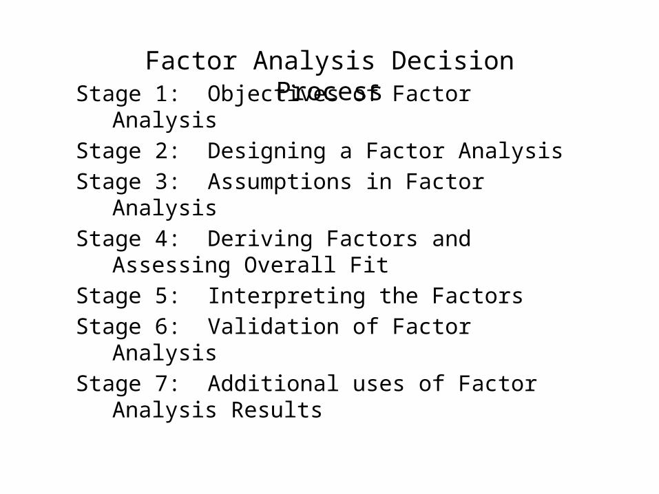
Factor Analysis Decision Process

Stage 1: Objectives of Factor Analysis

Stage 2: Designing a Factor Analysis

Stage 3: Assumptions in Factor Analysis

Stage 4: Deriving Factors and Assessing Overall Fit

Stage 5: Interpreting the Factors

Stage 6: Validation of Factor Analysis

Stage 7: Additional uses of Factor Analysis Results

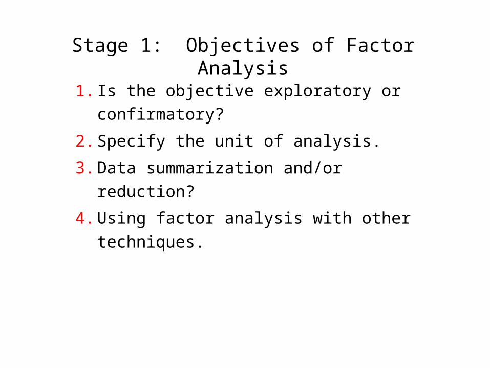
Stage 1: Objectives of Factor Analysis

1. Is the objective exploratory or confirmatory?

2. Specify the unit of analysis.

3. Data summarization and/or reduction?

4. Using factor analysis with other techniques.

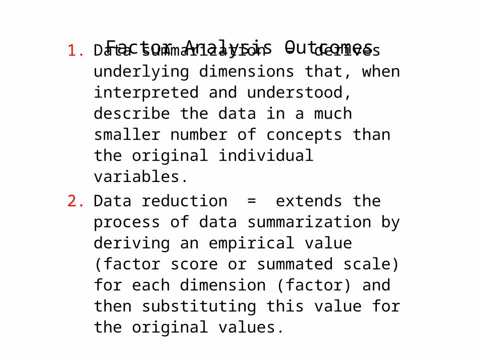
Factor Analysis Outcomes

1. Data summarization = derives underlying dimensions that, when interpreted and understood, describe the data in a much smaller number of concepts than the original individual variables.

2. Data reduction = extends the process of data summarization by deriving an empirical value (factor score or summated scale) for each dimension (factor) and then substituting this value for the original values.

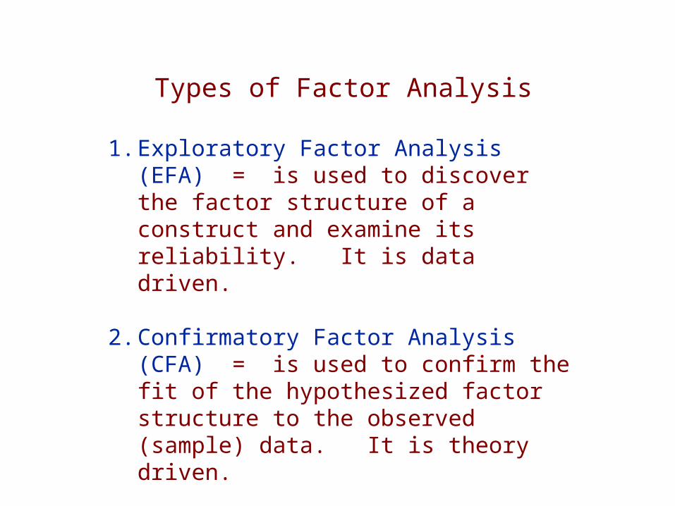
Types of Factor Analysis

1. Exploratory Factor Analysis (EFA) = is used to discover the factor structure of a construct and examine its reliability. It is data driven.

2. Confirmatory Factor Analysis (CFA) = is used to confirm the fit of the hypothesized factor structure to the observed (sample) data. It is theory driven.

Stage 2: Designing a Factor Analysis

Two Basic Decisions:

1. Design of study in terms of number of variables, measurement properties of variables, and the type of variables.

2. Sample size necessary.

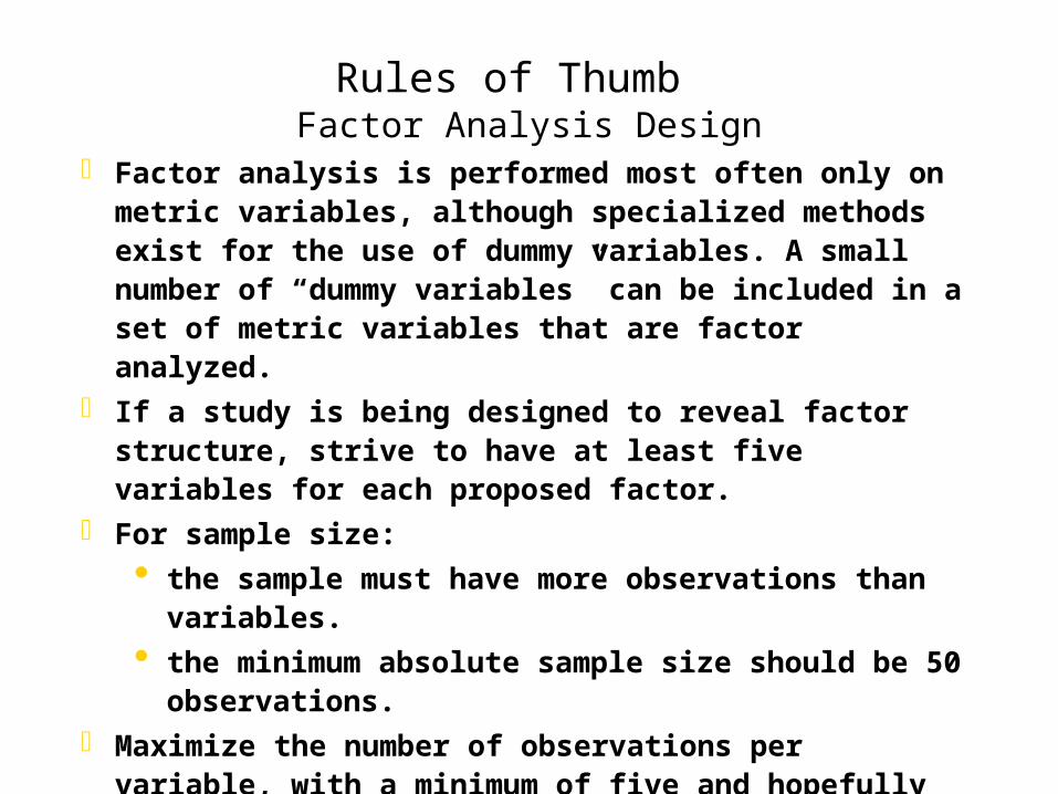
Rules of Thumb Factor Analysis Design

o Factor analysis is performed most often only on metric variables, although specialized methods exist for the use of dummy variables. A small number of “dummy variables” can be included in a set of metric variables that are factor analyzed.

o If a study is being designed to reveal factor structure, strive to have at least five variables for each proposed factor.

o For sample size:

• the sample must have more observations than variables.

• the minimum absolute sample size should be 50 observations.

o Maximize the number of observations per variable, with a minimum of five and hopefully at least ten observations per variable.

Stage 3: Assumptions in Factor Analysis

Two Basic Decisions . . .

1. Design of study in terms of number of variables, measurement properties of variables, and the type of variables.

2. Sample size required.

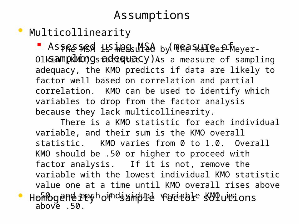
Assumptions• Multicollinearity

Assessed using MSA (measure of sampling adequacy).

• Homogeneity of sample factor solutions

The MSA is measured by the Kaiser-Meyer-Olkin (KMO) statistic. As a measure of sampling adequacy, the KMO predicts if data are likely to factor well based on correlation and partial correlation. KMO can be used to identify which variables to drop from the factor analysis because they lack multicollinearity. There is a KMO statistic for each individual variable, and their sum is the KMO overall statistic. KMO varies from 0 to 1.0. Overall KMO should be .50 or higher to proceed with factor analysis. If it is not, remove the variable with the lowest individual KMO statistic value one at a time until KMO overall rises above .50, and each individual variable KMO is above .50.

Rules of Thumb

Testing Assumptions of Factor Analysis

• There must be a strong conceptual foundation to support the assumption that a structure does exist before the factor analysis is performed.

• A statistically significant Bartlett’s test of sphericity (sig. < .05) indicates that sufficient correlations exist among the variables to proceed.

• Measure of Sampling Adequacy (MSA) values must exceed .50 for both the overall test and each individual variable. Variables with values less than .50 should be omitted from the factor analysis one at a time, with the smallest one being omitted each time.

Stage 4: Deriving Factors and Assessing Overall Fit

• Selecting the factor extraction method

– common vs. component analysis.

• Determining the number of factors to

represent the data.

Extraction Decisions

o Which method?

• Principal Components Analysis

• Common Factor Analysis

o How to rotate?

• Orthogonal or Oblique rotation

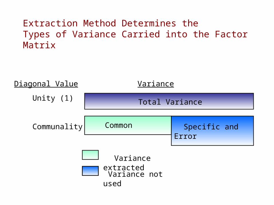
Extraction Method Determines the Types of Variance Carried into the Factor Matrix

Diagonal Value Variance

Unity (1)

Communality

Total Variance

Common Specific and Error

Variance extracted Variance not used

Principal Components vs. Common?

Two Criteria . . .

• Objectives of the factor analysis.

• Amount of prior knowledge about

the variance in the variables.

Number of Factors?

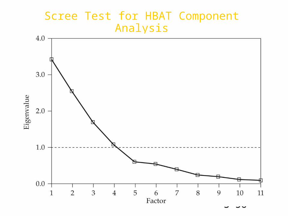
• A Priori Criterion• Latent Root Criterion• Percentage of Variance• Scree Test Criterion

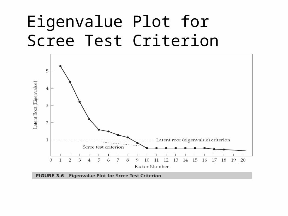
Eigenvalue Plot for Scree Test Criterion

Rules of Thumb

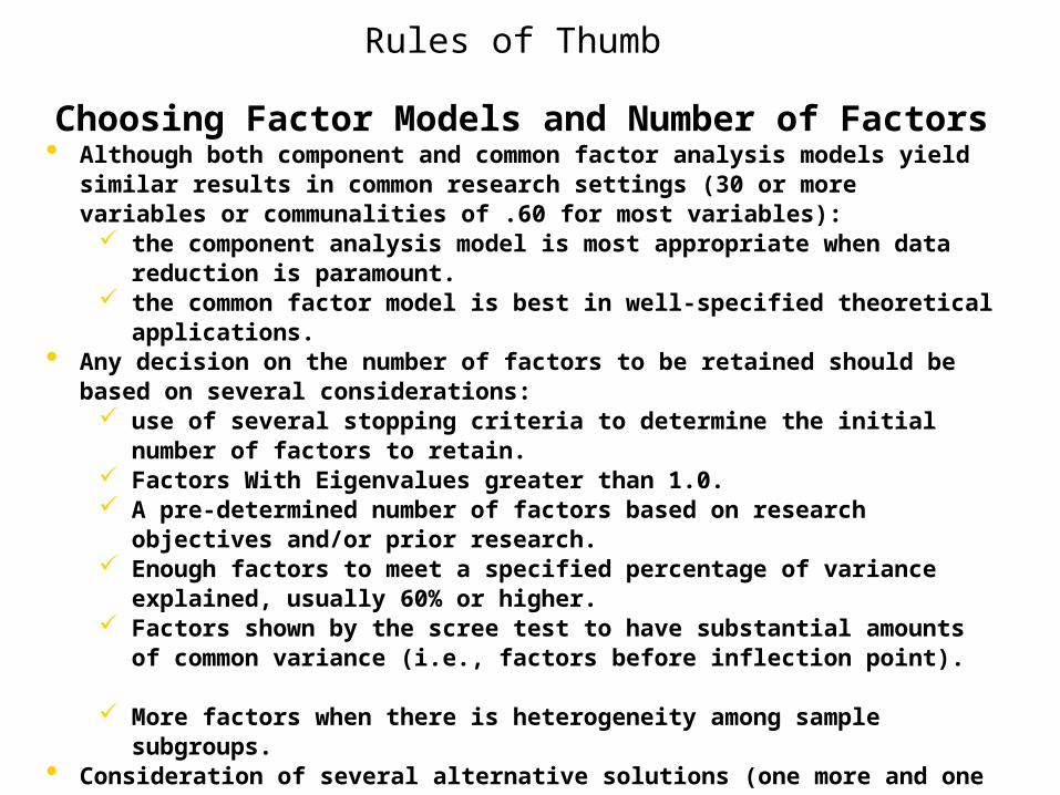
Choosing Factor Models and Number of Factors• Although both component and common factor analysis models yield similar

results in common research settings (30 or more variables or communalities of .60 for most variables):

the component analysis model is most appropriate when data reduction is paramount.

the common factor model is best in well-specified theoretical applications.• Any decision on the number of factors to be retained should be based on several

considerations: use of several stopping criteria to determine the initial number of factors to

retain. Factors With Eigenvalues greater than 1.0. A pre-determined number of factors based on research objectives and/or

prior research. Enough factors to meet a specified percentage of variance explained, usually

60% or higher. Factors shown by the scree test to have substantial amounts of common

variance (i.e., factors before inflection point). More factors when there is heterogeneity among sample subgroups.

• Consideration of several alternative solutions (one more and one less factor than the initial solution) to ensure the best structure is identified.

Processes of Factor Interpretation

• Estimate the Factor Matrix• Factor Rotation• Factor Interpretation• Respecification of factor model, if needed, may

involve . . .o Deletion of variables from analysiso Desire to use a different rotational approacho Need to extract a different number of factorso Desire to change method of extraction

Rotation of Factors

Factor rotation = the reference axes of the factors are turned about the origin until some other position has been reached. Since unrotated factor solutions extract factors based on how much variance they account for, with each subsequent factor accounting for less variance. The ultimate effect of rotating the factor matrix is to redistribute the variance from earlier factors to later ones to achieve a simpler, theoretically more meaningful factor pattern.

Two Rotational Approaches

1. Orthogonal = axes are maintained at 90 degrees.

2. Oblique = axes are not maintained at 90 degrees.

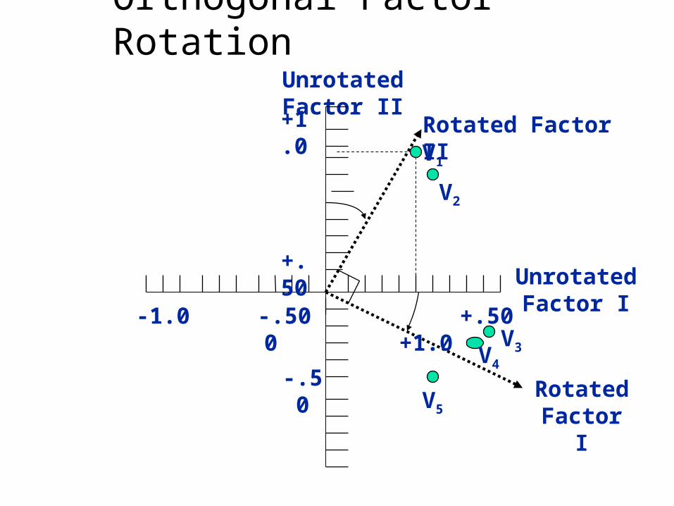
Orthogonal Factor RotationUnrotated Factor

II

Unrotated Factor I

Rotated Factor I

Rotated Factor II

-1.0 -.50 0

+.50 +1.0

-.50

-1.0

+1.0

+.50

V1

V2

V3V4

V5

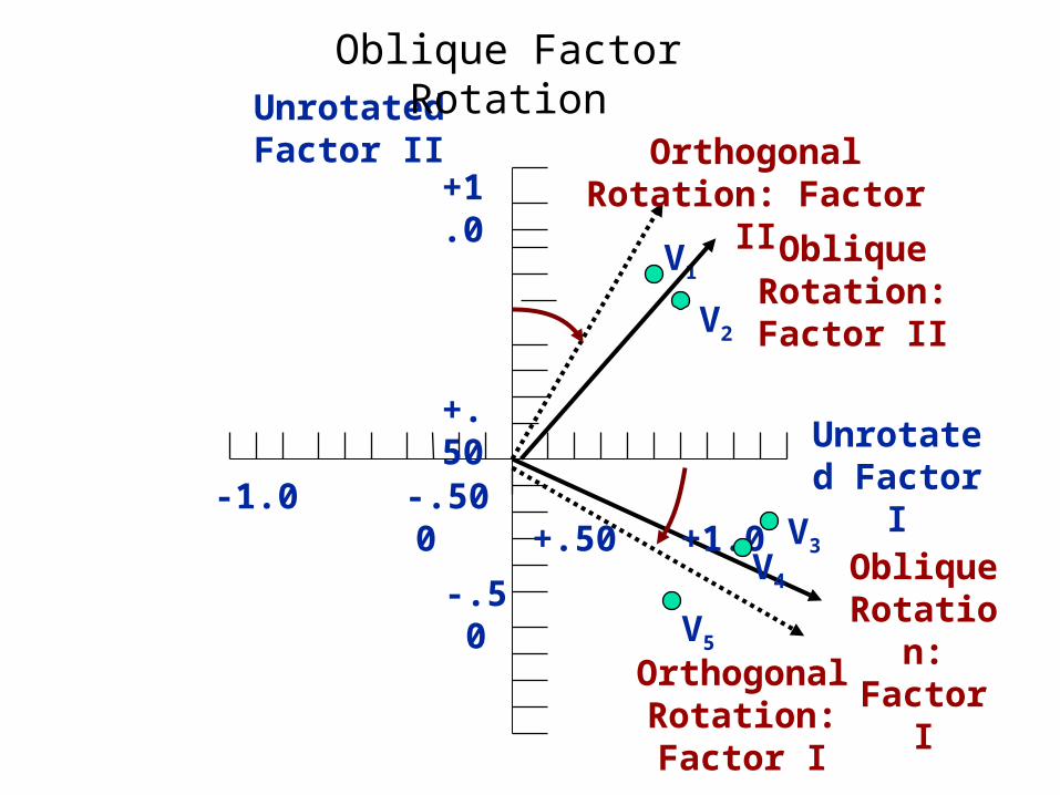
Unrotated Factor II

Unrotated Factor

IOblique Rotatio

n: Factor I

Orthogonal Rotation: Factor

II

-1.0 -.50 0

+.50 +1.0

-.50

-1.0

+1.0

+.50

V1

V2

V3V4

V5

Orthogonal Rotation: Factor I

Oblique Rotation: Factor II

Oblique Factor Rotation

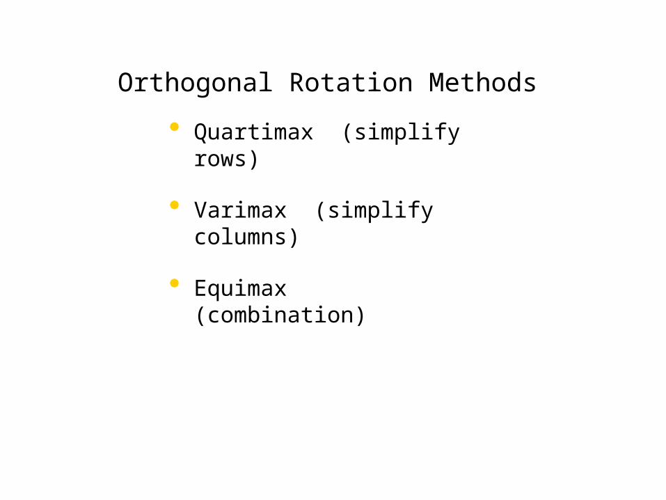
Orthogonal Rotation Methods

• Quartimax (simplify rows)

• Varimax (simplify columns)

• Equimax (combination)

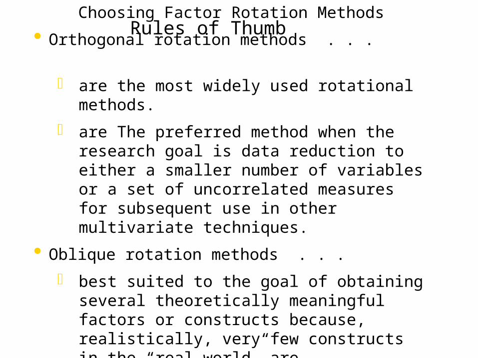
Rules of Thumb

Choosing Factor Rotation Methods

• Orthogonal rotation methods . . .

o are the most widely used rotational methods.

o are The preferred method when the research goal is data reduction to either a smaller number of variables or a set of uncorrelated measures for subsequent use in other multivariate techniques.

• Oblique rotation methods . . .

o best suited to the goal of obtaining several theoretically meaningful factors or constructs because, realistically, very few constructs in the “real world” are uncorrelated.

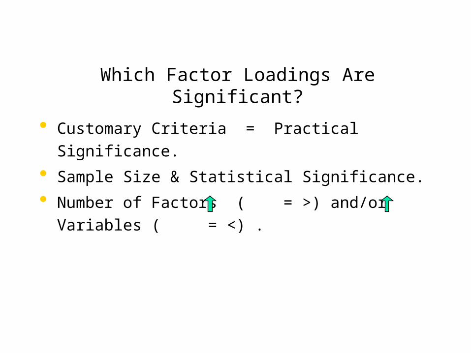
Which Factor Loadings Are Significant?

• Customary Criteria = Practical Significance.

• Sample Size & Statistical Significance.

• Number of Factors ( = >) and/or Variables ( = <) .

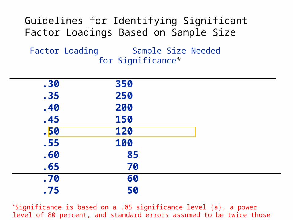
Guidelines for Identifying Significant Factor Loadings Based on Sample Size

Factor Loading Sample Size Needed for Significance*

.30 350

.35 250

.40 200

.45 150

.50 120

.55 100

.60 85

.65 70

.70 60

.75 50*Significance is based on a .05 significance level (a), a power level of 80 percent, and standard errors assumed to be twice those of conventional correlation coefficients.

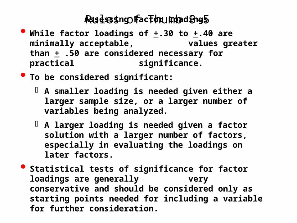
Rules of Thumb 3–5

Assessing Factor Loadings

• While factor loadings of +.30 to +.40 are minimally acceptable, values greater than + .50 are considered necessary for practical significance.

• To be considered significant:

o A smaller loading is needed given either a larger sample size, or a larger number of variables being analyzed.

o A larger loading is needed given a factor solution with a larger number of factors, especially in evaluating the loadings on later factors.

• Statistical tests of significance for factor loadings are generally very conservative and should be considered only as starting points needed for including a variable for further consideration.

Stage 5: Interpreting the Factors

• Selecting the factor extraction method

– common vs. component analysis.

• Determining the number of factors to

represent the data.

Interpreting a Factor Matrix:

1. Examine the factor matrix of loadings.

2. Identify the highest loading across all factors for each variable.

3. Assess communalities of the variables.

4. Label the factors.

Rules of Thumb 3–6

Interpreting The Factors

· An optimal structure exists when all variables have high loadings only on a single factor.

· Variables that cross-load (load highly on two or more factors) are usually deleted unless theoretically justified or the objective is strictly data reduction.

· Variables should generally have communalities of greater than .50 to be retained in the analysis.

· Respecification of a factor analysis can include options such as:

o deleting a variable(s),

o changing rotation methods, and/or

o increasing or decreasing the number of factors.

Stage 6: Validation of Factor Analysis

• Confirmatory Perspective.

• Assessing Factor Structure Stability.

• Detecting Influential Observations.

Stage 7: Additional Uses of Factor Analysis Results

• Selecting Surrogate Variables

• Creating Summated Scales

• Computing Factor Scores

Rules of ThumbSummated Scales

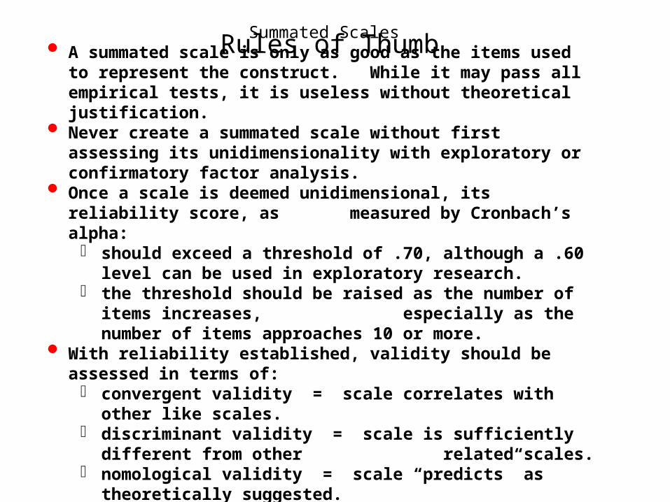
• A summated scale is only as good as the items used to represent the construct. While it may pass all empirical tests, it is useless without theoretical justification.

• Never create a summated scale without first assessing its unidimensionality with exploratory or confirmatory factor analysis.

• Once a scale is deemed unidimensional, its reliability score, as measured by Cronbach’s alpha:

o should exceed a threshold of .70, although a .60 level can be used in exploratory research.

o the threshold should be raised as the number of items increases, especially as the number of items approaches 10 or more.

• With reliability established, validity should be assessed in terms of:

o convergent validity = scale correlates with other like scales.o discriminant validity = scale is sufficiently different from

other related scales.o nomological validity = scale “predicts” as theoretically

suggested.

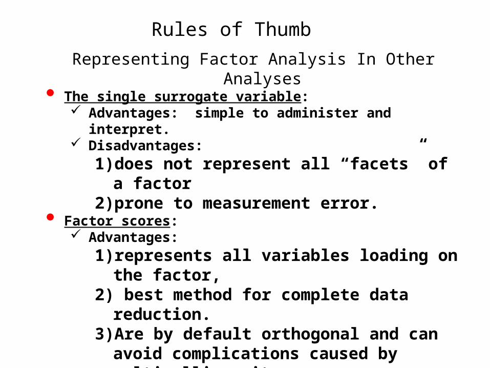
Rules of Thumb

Representing Factor Analysis In Other Analyses• The single surrogate variable:

Advantages: simple to administer and interpret. Disadvantages:

1) does not represent all “facets” of a factor 2) prone to measurement error.

• Factor scores: Advantages:

1) represents all variables loading on the factor,

2) best method for complete data reduction. 3) Are by default orthogonal and can avoid

complications caused by multicollinearity. Disadvantages:

1) interpretation more difficult since all variables contribute through loadings

2) Difficult to replicate across studies.

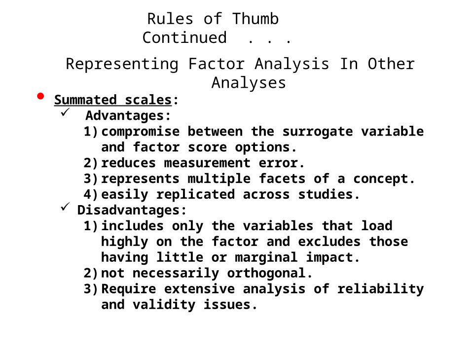
Rules of Thumb Continued . . .

Representing Factor Analysis In Other Analyses• Summated scales:

Advantages:1) compromise between the surrogate variable and factor

score options.2) reduces measurement error.3) represents multiple facets of a concept.4) easily replicated across studies.

Disadvantages:1) includes only the variables that load highly on the

factor and excludes those having little or marginal impact.

2) not necessarily orthogonal.3) Require extensive analysis of reliability and validity

issues.

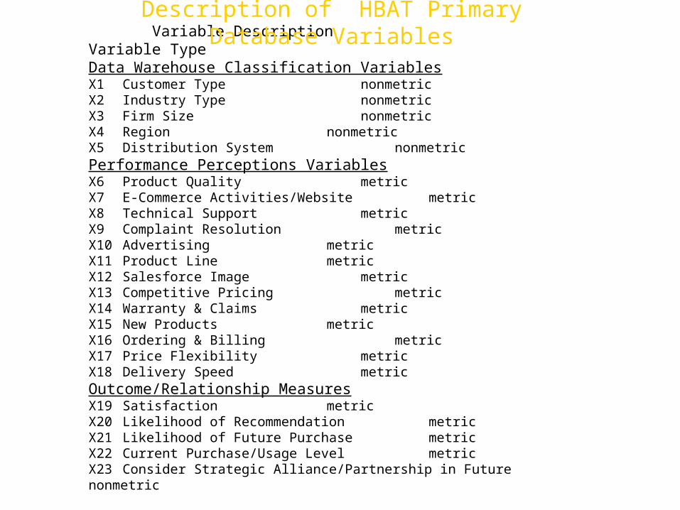
Variable Description Variable TypeData Warehouse Classification VariablesX1 Customer Type nonmetric X2 Industry Type nonmetric X3 Firm Size nonmetric X4 Region nonmetricX5 Distribution System nonmetricPerformance Perceptions VariablesX6 Product Quality metricX7 E-Commerce Activities/Website metricX8 Technical Support metricX9 Complaint Resolution metricX10 Advertising metricX11 Product Line metricX12 Salesforce Image metricX13 Competitive Pricing metricX14 Warranty & Claims metricX15 New Products metricX16 Ordering & Billing metricX17 Price Flexibility metricX18 Delivery Speed metricOutcome/Relationship MeasuresX19 Satisfaction metric X20 Likelihood of Recommendation metric X21 Likelihood of Future Purchase metric X22 Current Purchase/Usage Level metric X23 Consider Strategic Alliance/Partnership in Future nonmetric

Description of HBAT Primary Database Variables

3-55

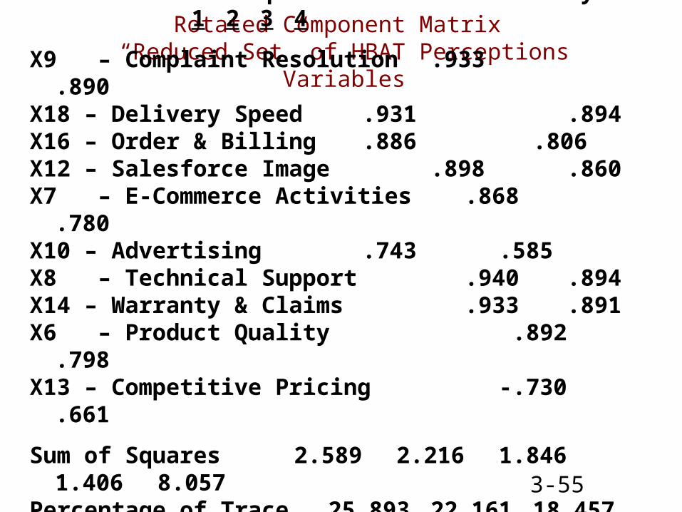
Rotated Component Matrix “Reduced Set” of HBAT Perceptions Variables

Component Communality

1 2 3 4

X9 – Complaint Resolution .933.890

X18 – Delivery Speed .931 .894X16 – Order & Billing .886 .806X12 – Salesforce Image .898

.860X7 – E-Commerce Activities .868

.780X10 – Advertising .743 .585X8 – Technical Support .940

.894X14 – Warranty & Claims .933

.891X6 – Product Quality

.892 .798X13 – Competitive Pricing -.730 .661

Sum of Squares 2.589 2.216 1.8461.406 8.057

Percentage of Trace 25.893 22.16118.457 14.061 80.572

Extraction Method: Principal Component Analysis. Rotation Method: Varimax.

3-56

Scree Test for HBAT Component Analysis

3-57

Factor Analysis Learning Checkpoint

1. What are the major uses of factor analysis?2. What is the difference between component

analysis and common factor analysis?3. Is rotation of factors necessary?4. How do you decide how many factors to extract?5. What is a significant factor loading?6. How and why do you name a factor?7. Should you use factor scores or summated ratings

in follow-up analyses?