Embed Size (px)
Citation preview

Applied Econometrics –Introduction to Time SeriesIntroduction to Time Series
Roman Horváth
Lecture 2

Contents
• Stationarity– What it is and what it is for
• Some basic time series models– Autoregressive (AR)– Moving average (MA)
2
– Moving average (MA)
• Consequences of non-stationarity (spurious regression)
• Testing for (non)-stationarity– Dickey-Fuller test– Augmented Dickey-Fuller test

• Xt is stationary if:• the series fluctuates around a constant long run
mean• Xt has finite variance which is not dependent upon time• Covariance between two values of Xt depends only on the difference apart in time (e.g. covariance between Xt and Xt-1 is
(Weak) Stationarity
3
difference apart in time (e.g. covariance between Xt and Xt-1 is the same as for Xt-8 and Xt-9)
E(Xt) = μ (mean is constant in t) Var(Xt) = σ2 (variance is constant in t)Cov(Xt ,Xt+k) = χ(k) (covariance is constant in t)
• If data not stationary, spurious regression problem

Examples of Times Series Models
• AR – autoregressive models Xt = β + α*Xt-1 + ut ……is called AR(1) process Xt = β + α1*Xt-1 + α2*Xt-2 +….+αk*Xt-k + ut …is AR(k) process
• MA – moving average models X = β + u + α *u ……is called MA(1) process
4
Xt = β + ut + α2*ut-1 ……is called MA(1) process Xt = β + ut + α2*ut-1 +….+αk*ut-k ….is called MA(k) process
• If you combine AR and MA process, you get ARMA process
• E.g. ARMA (1,1) is Xt = β +α*Xt-1+ut+ α2 ut-1

Is MA and AR process stationary?
• Compute mean, variance and covariance and check if it depends on time
• For AR process, you may easily derive that the process is stationary if α < 1
5
process is stationary if α < 1
• For MA (1) process, mean is β, variance is ut2
*(1+α22) and covariance cov(Xt , Xt-k) is either 0
if k>1 or ut2*α2 ,so it does not depend on time
(MA(k) is stationary process)
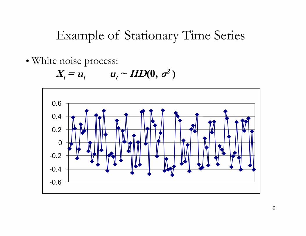
• White noise process:Xt = ut ut ~ IID(0, σ2 )
Example of Stationary Time Series
0.4
0.6
6
-0.6
-0.4
-0.2
0
0.2
0.4

Another Example of Stationary Time Series
Xt = 0.5*Xt-1 + ut ut ~ IID(0, σ2 )
Stationary without drift
0.6
0.8
7
-0.6
-0.4
-0.2
0
0.2
0.4
0.6

Example of Non-stationary Time Series
• Yt = α + β*t + ut , where t is time trend
• Take the expected value E(Y ) = α + β*t ,
8
• Take the expected value E(Yt ) = α + β*t , clearly the mean depends on time and the series is non-stationary

In contrast a non-stationary time series has at least one of the following characteristics:• Does not have a long run mean which the series returns
Non-stationary time series
9
returns• Variance is dependent upon time and goes to infinity as the sample period approaches infinity• Correlogram does not die out - long memory

Example of Non-stationary Time Series
UK GDP Level
6080
100120
10
• The level of GDP is not constant; the mean increases over time.
0204060
1992
Q3
1993
Q2
1994
Q1
1994
Q4
1995
Q3
1996
Q2
1997
Q1
1997
Q4
1998
Q3
1999
Q2
2000
Q1
2000
Q4
2001
Q3
2002
Q2
2003
Q1

Non-stationary time series – correlogram
UK GDP (Yt)
0.5
0.6
0.7
0.8
0.9
1.0ACF-Y
11
• For non-stationary series the Autocorrelation Function (ACF) declines towards zero at a slow rate as k increases.
0 1 2 3 4 5 6 7
0.1
0.2
0.3
0.4
0.5

• Some transformation = first differenece, logarithm, second difference ...•First difference of UK GDP (ΔYt = Yt - Yt-1) is stationary:
- growth rate is reasonably constant through time- variance is also reasonably constant through time
Possible solutions of non-stationarity
1.4
12
00.20.40.60.8
11.21.4
1992
Q3
1993
Q2
1994
Q1
1994
Q4
1995
Q3
1996
Q2
1997
Q1
1997
Q4
1998
Q3
1999
Q2
2000
Q1
2000
Q4
2001
Q3
2002
Q2
2003
Q1

Stationary time series - correlogram
UK GDP Growth (Δ Yt)
0.25
0.50
0.75
1.00ACF-DY
13
• ACF decline towards zero as k increases• Decline of ACF is rapid for stationary series
0 1 2 3 4 5 6 7
-0.75
-0.50
-0.25
0.00

Non-stationary Time Series Continued –Random Walk
• Xt = Xt-1 + ut , where ut ~ IID(0, σ2 )• Mean is constant in t: E(Xt) = E(Xt-1)
X1 = X0 + u1 (take initial value X0)
14
X1 = X0 + u1 (take initial value X0)X2 = X1 + u2 = (X0 + u1 ) + u2
…Xt = X0 + u1 + u2 +…+ ut (take expectations)
E(Xt) = E(X0 + u1 + u2 +…+ ut) = E(X0) = constant
• Variance is not constant in t: Var(Xt) = Var(X0) + Var(u1) +…+ Var(ut)
= 0 + σ2 +…+ σ2 = t σ2
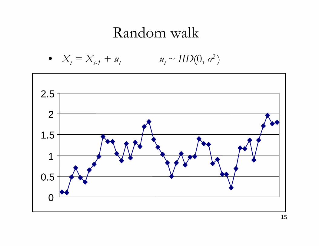
Random walk
2
2.5
• Xt = Xt-1 + ut ut ~ IID(0, σ2 )
15
0
0.5
1
1.5

• AR(1) process: Xt = + α Xt-1 + ut ;(ut ~ IID(0, σ2 ))α < 1stationary process - “process forgets
past”α = 1non-stationary process - “process does
Relationship between stationary and non-stationary process
16
α = 1non-stationary process - “process does not forget past”
= 0 without drift 0 with drift
• MA process is always stationary

Summary on basic time series processes
• AR (k) process
• MA(k) process
• ARMA (p,l) process
• If you k-th difference the data, then you have
17
• If you k-th difference the data, then you have ARIMA (p,k,l) – estimation of ARIMA models is a subject of next lecture

Spurious Regression ( spurious correlation)
• Problem that time-series data usually includes trend• Result:
– Spurious correlation (variables with similar trends are correlated)
18
are correlated)– Spurious regression (independent variable with
similar trend looks as dependent = strong statistical relationship)
coefficient significant (high adjusted-R2, large t-statistics) ... even if unrelated in economic terms

How to avoid spurious regression: 3 approaches to non-stationarity
1. Include a time trend as an independent variable (old-fashioned) yt = c + 1xt + 2t + ut .....(t = 1,2, ..., T)
2. 1st difference the data if variables I(1); 2nd difference if I(2)
= converts non-stationary variables into stationary
19
= converts non-stationary variables into stationary variables
Problems: – theory often about levels– detrending loss of information
3. Cointegration + ECM= Long-run relationship + short-run adjustment

(A) Informal methods:- Plot time series- Correlogram
How do we identify non-stationary processes?
20
- Correlogram
(B) Formal methods:- Statistical test for stationarity- Dickey-Fuller tests.

Informal Procedures to identify non-stationary processes
(a) Constant mean?
2
4
6
8
10
12RW2
21
(b) Constant variance?
0 50 100 150 200 250 300 350 400 450 500
-200
-150
-100
-50
0
50
100
150
200var
0 50 100 150 200 250 300 350 400 450 500
0
2

Informal Procedures to identify non-stationary processes
• Diagnostic test – Correlogram for stationary process (dies out rapidly, series has no memory)
0.00
0.25
0.50whitenoise
22
0 50 100 150 200 250 300 350 400 450 500
-0.25
0 5 10
-0.5
0.0
0.5
1.0ACF-whitenoise

Informal Procedures to identify non-stationary processes
• Diagnostic test – Correlogram for a random walk (does not die out, high autocorrelation for large values of k)
5.0
7.5
10.0
12.5randomwalk
23
0 50 100 150 200 250 300 350 400 450 500
0.0
2.5
5.0
0 5 10
0.25
0.50
0.75
1.00ACF-randomwalk

Dickey-Fuller Test
• Test based on Yt = Yt-1 + ut
- DF test to determine whether =1
• Yes unit root non-stationary
• No no unit root
24
• Dynamic model:
– Subtract Yt-1 ... Yt - Yt-1 = (-1)Yt-1 + ut
– Reparameterise: Yt = Yt-1 + ut
where = (-1)
– Test =0 equivalent to test =1
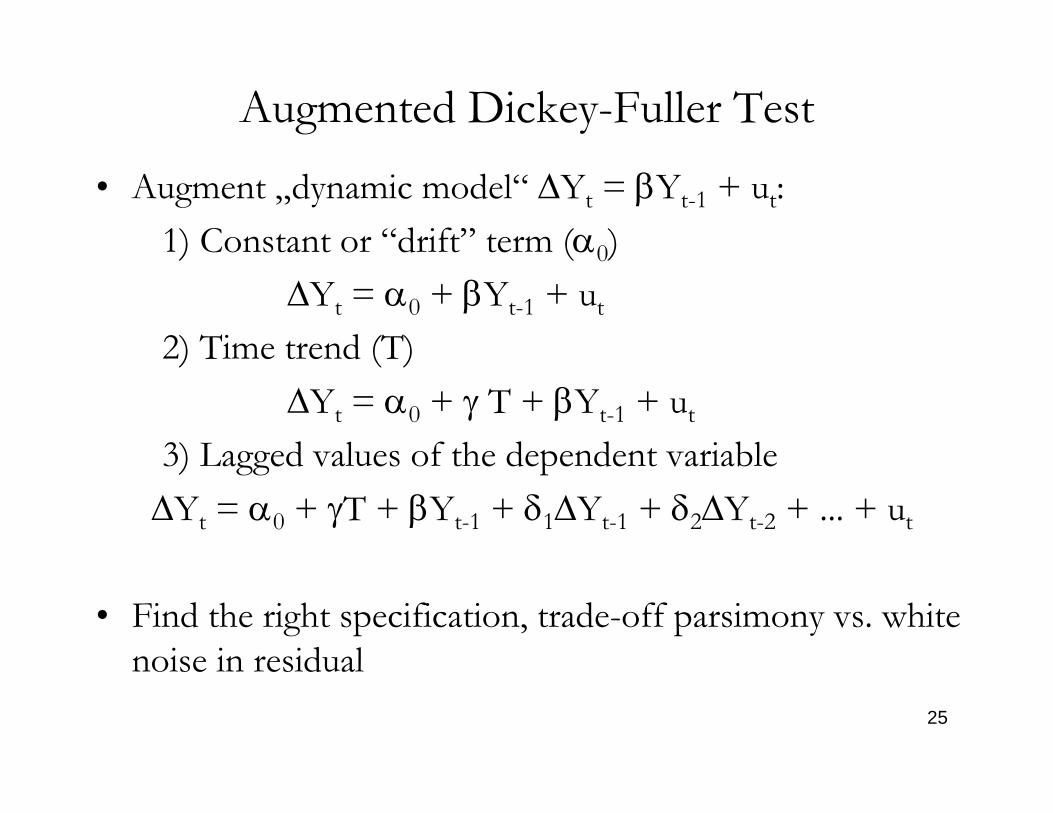
Augmented Dickey-Fuller Test
• Augment „dynamic model“ Yt = Yt-1 + ut:
1) Constant or “drift” term (0)
Yt = 0 + Yt-1 + ut
2) Time trend (T)
Yt = 0 + T + Yt-1 + ut
25
Yt = 0 + T + Yt-1 + ut
3) Lagged values of the dependent variable
Yt = 0 + T + Yt-1 + 1Yt-1 + 2Yt-2 + ... + ut
• Find the right specification, trade-off parsimony vs. white noise in residual

Critical values• DF/ADF use t- and F-statistics but critical values are
not standard
• Problems:
• distributions of these statistics are non-standard
• special tables of critical values (derived from
26
• special tables of critical values (derived from numerical simulations)
• Usual t- and F-tests not valid in presence of unit roots


![Jozef Barunik - Total, asymmetric and frequency ......Corresponding author, Tel. +420(776)259273, Email address: barunik@fsv.cuni.cz 1 converges in probability to [p t;p t] with n!1](https://img.pdfslide.us/doc/110x75/60f724aeca63b560d9422426/jozef-barunik-total-asymmetric-and-frequency-corresponding-author-tel.jpg)