Econometrics

Week 6

Institute of Economic StudiesFaculty of Social Sciences

Charles University in Prague

Fall 2012

1 / 21

Recommended Reading

For the todayAdvanced Panel Data Methods.Chapter 14 (pp. 441 – 460).

For the next weekMIDTERM

In the 2 weeksInstrumental Variables Estimation and Two Stage LeastSquaresChapter 15 (pp. 461 – 491).

2 / 21

Today’s Talk

Last week we have learned about the independentlypooled cross sections and panel data.We have learned a common method of estimation firstdifferencing.Today, we will continue and introduce two methods forestimation of the Panel data.

Fixed Effects Estimator.Random Effects Estimator.

3 / 21

Fixed Effects Estimation

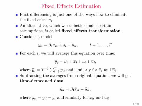
First differencing is just one of the ways how to eliminatethe fixed effect ai.An alternative, which works better under certainassumptions, is called fixed effects transformation.Consider a model:

yit = β1xit + ai + uit, t = 1, . . . , T.

For each i, we will average this equation over time:

yi = β1 + xi + ai + ui,

where yi = T−1∑T

t=1 yit and similarly for xi and ui

Subtracting the averages from original equation, we will gettime-demeaned data:

yit = β1xit + uit,

where yit = yit − yi and similarly for xit and uit

4 / 21

Fixed Effects Estimation cont.

The fixed effects transformation is also called withintransformation.Unobserved effects ai disappeared ⇒ we can use pooledOLS.Pooled OLS estimator on the time-demeaned variables iscalled fixed effects estimator, or within estimator.name “within” comes from the fact that we use timevariation within each cross-sectional observation.We also know a between estimator, which is obtained asthe OLS estimator of yi = β0 + β1xi + ai + ui.We use time-averages and then run a cross-sectionalregression.Between estimator is biased when ai is correlated with xi

5 / 21

Fixed Effects Estimation cont.

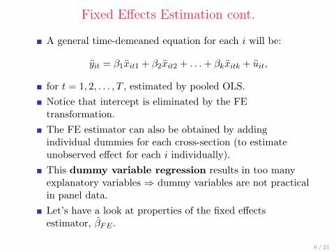
A general time-demeaned equation for each i will be:

yit = β1xit1 + β2xit2 + . . .+ βkxitk + uit,

for t = 1, 2, . . . , T , estimated by pooled OLS.Notice that intercept is eliminated by the FEtransformation.The FE estimator can also be obtained by addingindividual dummies for each cross-section (to estimateunobserved effect for each i individually).This dummy variable regression results in too manyexplanatory variables ⇒ dummy variables are not practicalin panel data.Let’s have a look at properties of the fixed effectsestimator, βFE .

6 / 21

Assumptions for Fixed Effects Estimator

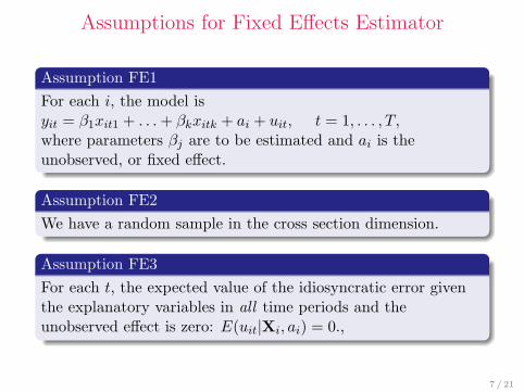
Assumption FE1For each i, the model isyit = β1xit1 + . . .+ βkxitk + ai + uit, t = 1, . . . , T,where parameters βj are to be estimated and ai is theunobserved, or fixed effect.

Assumption FE2We have a random sample in the cross section dimension.

Assumption FE3For each t, the expected value of the idiosyncratic error giventhe explanatory variables in all time periods and theunobserved effect is zero: E(uit|Xi, ai) = 0.,

7 / 21

Assumptions for Fixed Effects Estimator cont.

Assumption FE4

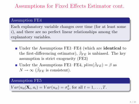
Each explanatory variable changes over time (for at least somei), and there are no perfect linear relationships among theexplanatory variables.

Under the Assumptions FE1–FE4 (which are identical tothe first-differencing estimator), βFE is unbiased. The keyassumption is strict exogeneity (FE3)Under the Assumptions FE1–FE4, plim(βFE) = β asN →∞ (βFE is consistent).

Assumption FE5

V ar(uit|Xi, ai) = V ar(uit) = σ2u, for all t = 1, . . . , T .

8 / 21

Assumptions for Fixed Effects Estimator cont.

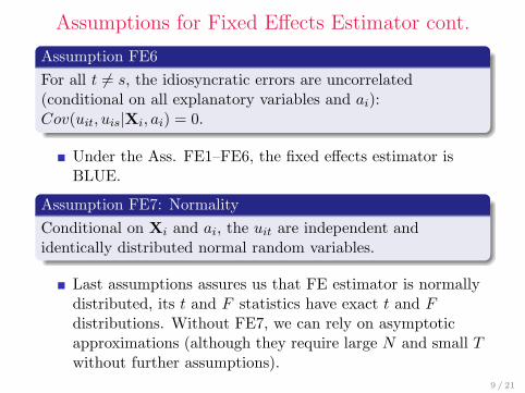
Assumption FE6For all t 6= s, the idiosyncratic errors are uncorrelated(conditional on all explanatory variables and ai):Cov(uit, uis|Xi, ai) = 0.

Under the Ass. FE1–FE6, the fixed effects estimator isBLUE.

Assumption FE7: NormalityConditional on Xi and ai, the uit are independent andidentically distributed normal random variables.

Last assumptions assures us that FE estimator is normallydistributed, its t and F statistics have exact t and Fdistributions. Without FE7, we can rely on asymptoticapproximations (although they require large N and small Twithout further assumptions).

9 / 21

Fixed Effects (FE) vs. First Differencing (FD)

FD involves differencing the data, FE involvestime-demeaning. Which one to use?FD and FE estimates and statistics are identical whenT = 2.For T ≥ 2, the methods are different.If uit are uncorrelated, FE is more efficient than FD.If uit follow i.e. Random Walk, then ∆uit are uncorrelatedand FD is better ⇒ test whether ∆uit are seriallycorrelated first.But in most of the data serial correlation is not that strongas in Random Walk.Thus it is suggested to obtain both estimates. If the resultsare not sensitive, then it is fine. But if they vary, we haveto find out why!

10 / 21

Fixed Effects with Unbalanced Panels

Panel data have often missing years for some cross-sections.These data are called unbalanced panel.We simply use the time-demeaning of Ti observations intime for each cross-section i and FE is equivalent to an FEon balanced panel.But we should know the reason, why we have unbalancedpanel.Provided the reason we have missing data for some i is notcorrelated with uit, unbalanced panel cause no problem.But if we have for example missing data of some firmsbecause of merger of 2 firms, or because they have gone outof the business, we have nonrandom sample.The reason of firm leaving the sample is correlated withunobserved factors in time and thus affects uit ⇒ bias.The problem is more complicated ⇒ Master course.

11 / 21

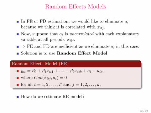
Random Effects Models

In FE or FD estimation, we would like to eliminate ai

because we think it is correlated with xitj ,Now, suppose that ai is uncorrelated with each explanatoryvariable at all periods, xitj .⇒ FE and FD are inefficient as we eliminate ai in this case.Solution is to use Random Effect Model

Random Effects Model (RE)

yit = β0 + β1xit1 + . . .+ βkxitk + ai + uit,where Cov(xitj , ai) = 0for all t = 1, 2, . . . , T and j = 1, 2, . . . , k.

How do we estimate RE model?

12 / 21

Random Effects Models cont.

It is important to see that if we believe that ai isuncorrelated with explanatory variables, OLS of simplecross-sections is constistent.Thus we may not need panel data at all.But, in this case, we throw away useful information in theother time periods.If we want to use this information, we can use pooled OLSestimation.But pooled OLS ignores the key feature of the model -serial correlation in the error term.

13 / 21

Random Effects Models cont.

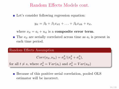
Let’s consider following regression equation:

yit = β0 + β1xit1 + . . .+ βkxitk + νit,

where νit = ai + uit is a composite error term.The νit are serially correlated across time as ai is present ineach time period.

Random Effects Assumption

Corr(νit, νis) = σ2a/(σ

2a + σ2

u),

for all t 6= s, where σ2a = V ar(ai) and σ2

u = V ar(uit)

Because of this positive serial correlation, pooled OLSestimator will be incorrect.

14 / 21

Random Effects Models cont.

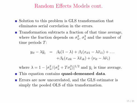
Solution to this problem is GLS transformation thateliminates serial correlation in the errors.Transformation subtracts a fraction of that time average,where the fraction depends on σ2

u, σ2a and the number of

time periods T :

yit − λyi = β0(1− λ) + β1(xit1 − λxi1) + . . .

+βk(xitk − λxik) + (νit − λνi)

where λ = 1− [σ2u/(σ

2u + Tσ2

a)]1/2 and yi is time average.This equation contains quasi-demeaned data.Errors are now uncorrelated, and the GLS estimator issimply the pooled OLS of this transformation.

15 / 21

Random Effects Models cont.

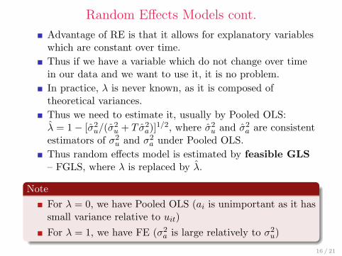
Advantage of RE is that it allows for explanatory variableswhich are constant over time.Thus if we have a variable which do not change over timein our data and we want to use it, it is no problem.In practice, λ is never known, as it is composed oftheoretical variances.Thus we need to estimate it, usually by Pooled OLS:λ = 1− [σ2

u/(σ2u + T σ2

a)]1/2, where σ2u and σ2

a are consistentestimators of σ2

u and σ2a under Pooled OLS.

Thus random effects model is estimated by feasible GLS– FGLS, where λ is replaced by λ.

NoteFor λ = 0, we have Pooled OLS (ai is unimportant as it hassmall variance relative to uit)For λ = 1, we have FE (σ2

a is large relatively to σ2u)

16 / 21

Assumptions for Random Effects

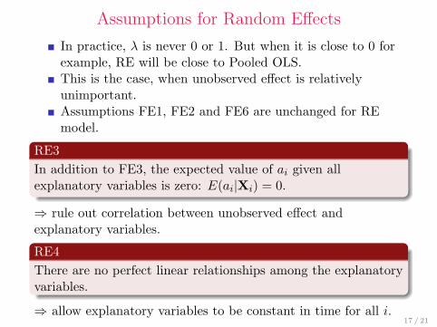
In practice, λ is never 0 or 1. But when it is close to 0 forexample, RE will be close to Pooled OLS.This is the case, when unobserved effect is relativelyunimportant.Assumptions FE1, FE2 and FE6 are unchanged for REmodel.

RE3In addition to FE3, the expected value of ai given allexplanatory variables is zero: E(ai|Xi) = 0.

⇒ rule out correlation between unobserved effect andexplanatory variables.

RE4There are no perfect linear relationships among the explanatoryvariables.

⇒ allow explanatory variables to be constant in time for all i.17 / 21

Assumptions for Random Effects cont.

RE5In addition to FE5, the variance of ai given all explanatoryvariables is constant: V ar(ai|Xi) = σ2

a.

Under the Assumptions FE1, FE2, RE3 and RE4, therandom effects estimator βRE is consistent as N gets largefor fixed T .RE estimator is not unbiased unless we know λ.RE estimator is also approximately normally distributedwith large N and usual standard errors, t statistics and Fstatistics are valid.

18 / 21

Fixed Effects vs. Random Effects

We decide whether to use RE or FE based on ai.If unobserved effect is something we want to estimate, useFE. (i.e. Panel Data for EU-27).If unobserved effect is supposed to be random, use RE (i.e.Panel Data for schools in large country).But, to treat ai as random, we have to make sure that it isnot correlated with explanatory variable.If unobserved effect ai is correlated with explanatoryvariables, FE is consistent, while RE is inconsistent.Otherwise, RE is more efficient that FE.

19 / 21

Fixed Effects vs. Random Effects cont.

Thus we can test whether to use FE or RE statistically:

Haussman testH0 : cov(ai, xit) = 0Under the null, both FE and RE are consistent, butRE is asymptotically more efficient.Under the alternative, FE is still consistent (RE is not).

We can test and correct for serial correlation andheteroskedasticity in the errors.We can estimate standard errors robust to both.

20 / 21

Thank you

Thank you very much for your attention!

21 / 21