Econometrics

Week 3

Institute of Economic StudiesFaculty of Social Sciences

Charles University in Prague

Fall 2012

1 / 23

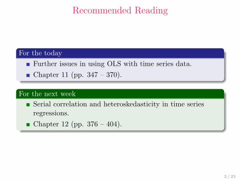
Recommended Reading

For the todayFurther issues in using OLS with time series data.Chapter 11 (pp. 347 – 370).

For the next weekSerial correlation and heteroskedasticity in time seriesregressions.Chapter 12 (pp. 376 – 404).

2 / 23

Today’s Lecture

We have learned that OLS has exactly same desirable finitesample properties in the time-series case as in thecross-sectional case.But we need somewhat altered set of assumptions.Today, we will study the large sample properties, which aremuch more problematic in time-series than incross-sectional case.I will introduce the key concepts needed to apply the usuallarge sample approximations in regression analysis withtime series.Trend analysis - crucial in economic analysis, most of thetime, you will deal with these data.

3 / 23

Stationary and Nonstationary Time Series

A stationary process is important for time series analysis.PDF of stationary process is stable over time.If we shift the sequence of the collection of randomvariables in any time, joint probability distribution mustremain unchanged.

Stationarity

The stochastic process {xt : t = 1, 2, . . .} is stationary if forevery collection of time indices 1 ≤ t1 < t2 < . . . < tm, the jointprobability distribution of (xt1 , xt2 , . . . , xtm) is the same as thejoint probability distribution of (xt1+h, xt2+h, . . . , xtm+h) for allintegers h ≥ 1.

Definition may seem little abstract, but meaning is prettystraightforward ⇒ see example on the next page.Time series with trend are nonstationary ⇒ its meanchanges in time.

4 / 23

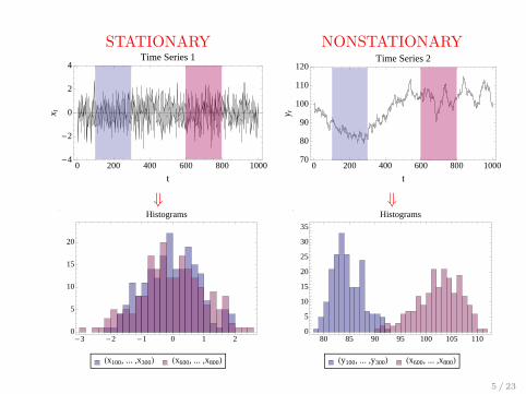
STATIONARY NONSTATIONARY

0 200 400 600 800 1000-4

-2

0

2

4

t

x tTime Series 1

0 200 400 600 800 100070

80

90

100

110

120

t

y t

Time Series 2

⇓ ⇓

-3 -2 -1 0 1 20

5

10

15

20

Histograms

Hx100, ... ,x300L Hx600, ... ,x800L

80 85 90 95 100 105 1100

5

10

15

20

25

30

35

Histograms

Hy100, ... ,y300L Hx600, ... ,x800L

5 / 23

Covariance Stationary Process

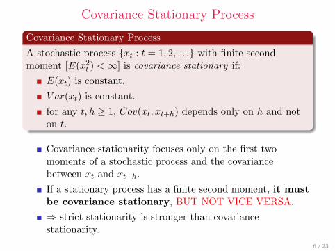
Covariance Stationary Process

A stochastic process {xt : t = 1, 2, . . .} with finite secondmoment [E(x2

t ) <∞] is covariance stationary if:E(xt) is constant.V ar(xt) is constant.for any t, h ≥ 1, Cov(xt, xt+h) depends only on h and noton t.

Covariance stationarity focuses only on the first twomoments of a stochastic process and the covariancebetween xt and xt+h.If a stationary process has a finite second moment, it mustbe covariance stationary, BUT NOT VICE VERSA.⇒ strict stationarity is stronger than covariancestationarity.

6 / 23

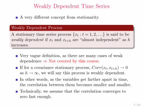
Weakly Dependent Time Series

A very different concept from stationarity.

Weakly Dependent Process

A stationary time series process {xt : t = 1, 2, . . .} is said to beweakly dependent if xt and xt+h are “almost independent” as hincreases.

Very vague definition, as there are many cases of weakdependence ⇒ Not covered by this course.If for a covariance stationary process, Corr(xt, xt+h)→ 0as h→∞, we will say this process is weakly dependent.In other words, as the variables get farther apart in time,the correlation between them becomes smaller and smaller.Technically, we assume that the correlation converges tozero fast enough.

7 / 23

Weakly Dependent Time Series cont.

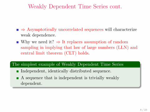
⇒ Asymptotically uncorrelated sequences will characterizeweak dependence.Why we need it? ⇒ It replaces assumption of randomsampling in implying that law of large numbers (LLN) andcentral limit theorem (CLT) holds.

The simplest example of Weakly Dependent Time SeriesIndependent, identically distributed sequence.A sequence that is independent is trivially weaklydependent.

8 / 23

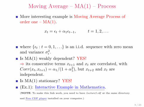
Moving Average – MA(1) – Process

More interesting example is Moving Average Process oforder one – MA(1).

xt = εt + α1εt−1, t = 1, 2, . . .

where {εt : t = 0, 1, . . .} is an i.i.d. sequence with zero meanand variance σ2

ε .Is MA(1) weakly dependent? YES!⇒ its consecutive terms xt+1 and xt are correlated, withCorr(xt, xt+1) = α1/(1 + α2

1), but xt+2 and xt areindependent.Is MA(1) stationary? YES!(Ex.1): Interactive Example in Mathematica.(NOTE: To make this link work, you need to have Lecture3.cdf at the same directory

and Free CDF player installed on your computer.)

9 / 23

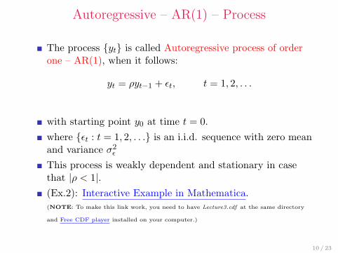
Autoregressive – AR(1) – Process

The process {yt} is called Autoregressive process of orderone – AR(1), when it follows:

yt = ρyt−1 + εt, t = 1, 2, . . .

with starting point y0 at time t = 0.where {εt : t = 1, 2, . . .} is an i.i.d. sequence with zero meanand variance σ2

ε

This process is weakly dependent and stationary in casethat |ρ < 1|.(Ex.2): Interactive Example in Mathematica.(NOTE: To make this link work, you need to have Lecture3.cdf at the same directory

and Free CDF player installed on your computer.)

10 / 23

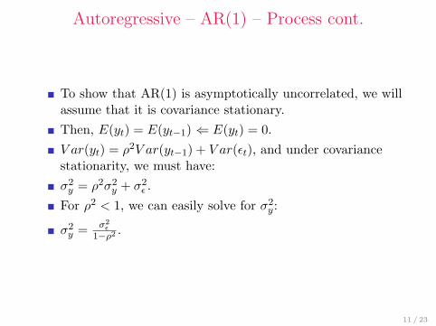
Autoregressive – AR(1) – Process cont.

To show that AR(1) is asymptotically uncorrelated, we willassume that it is covariance stationary.Then, E(yt) = E(yt−1) ⇐ E(yt) = 0.V ar(yt) = ρ2V ar(yt−1) + V ar(εt), and under covariancestationarity, we must have:σ2y = ρ2σ2

y + σ2ε .

For ρ2 < 1, we can easily solve for σ2y :

σ2y = σ2

ε1−ρ2 .

11 / 23

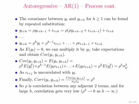
Autoregressive – AR(1) – Process cont.

The covariance between yt and yt+h for h ≥ 1 can be foundby repeated substitution:yt+h = ρyt+h−1 + εt+h = ρ(ρyt+h−2 + εt+h−1) + εt+h

. . .

yt+h = ρhyt + ρh−1εt+1 + . . .+ ρεt+h−1 + εt+h

As E(yt) = 0, we can multiply it by yt, take expectationsand obtain Cov(yt, yt+h).Cov(yt, yt+h) = E(yt, yt+h) =ρhE(y2

t )+ρh−1E(ytεt+1)+. . .+E(ytεt+h) = ρhE(y2t ) = ρhσ2

y .As εt+j is uncorrelated with yt.

Finally, Corr(yt, yt+h) = Cov(yt,yt+h)σyσy

= ρh

So ρ is correlation between any adjacent 2 terms, and forlarge h, correlation gets very low (ρh → 0 as h→∞.)

12 / 23

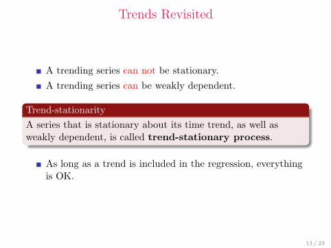
Trends Revisited

A trending series can not be stationary.A trending series can be weakly dependent.

Trend-stationarityA series that is stationary about its time trend, as well asweakly dependent, is called trend-stationary process.

As long as a trend is included in the regression, everythingis OK.

13 / 23

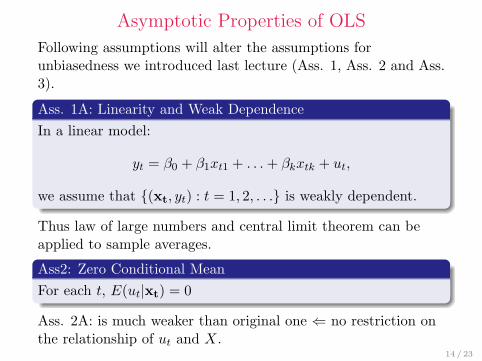
Asymptotic Properties of OLS

Following assumptions will alter the assumptions forunbiasedness we introduced last lecture (Ass. 1, Ass. 2 and Ass.3).

Ass. 1A: Linearity and Weak DependenceIn a linear model:

yt = β0 + β1xt1 + . . .+ βkxtk + ut,

we assume that {(xt, yt) : t = 1, 2, . . .} is weakly dependent.

Thus law of large numbers and central limit theorem can beapplied to sample averages.

Ass2: Zero Conditional MeanFor each t, E(ut|xt) = 0

Ass. 2A: is much weaker than original one ⇐ no restriction onthe relationship of ut and X.

14 / 23

Asymptotic Properties of OLS cont.

Ass. 3A: No Perfect CollinearityNo independent variable is constant or a perfect linearcombination of the others. remains the same

Theorem 1: Consistency of OLS

Under Ass. (1A), (2A) and (3A), the OLS estimators areconsistent: plim β̂j = βj , j = 0, 1, . . . , k.

The theorem is similar to the one we used in cross-sectionaldata, but we have omitted random sampling assumption(thanks to the Ass 2.).

15 / 23

Large-Sample Inference

We have weaker Ass. 4 and Ass. 5 than in CLM counterpart:

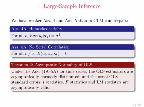
Ass. 4A: Homoskedasticity

For all t, V ar(ut|xt) = σ2.

Ass. 5A: No Serial CorrelationFor all t 6= s, E(ut, us|xt) = 0

Theorem 2: Asymptotic Normality of OLS

Under the Ass. (1A–5A) for time series, the OLS estimators areasymptotically normally distributed, and the usual OLSstandard errors, t statistics, F statistics and LM statistics areasymptotically valid.

16 / 23

Large-Sample Inference

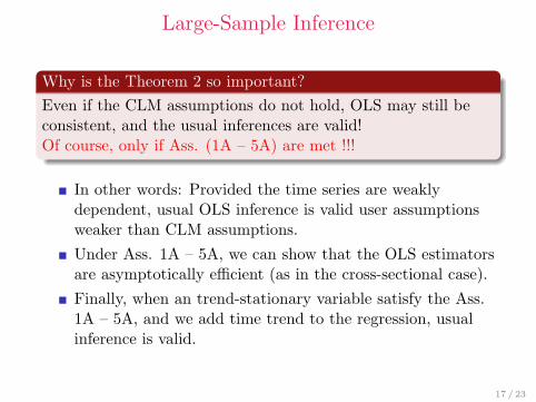
Why is the Theorem 2 so important?Even if the CLM assumptions do not hold, OLS may still beconsistent, and the usual inferences are valid!Of course, only if Ass. (1A – 5A) are met !!!

In other words: Provided the time series are weaklydependent, usual OLS inference is valid user assumptionsweaker than CLM assumptions.Under Ass. 1A – 5A, we can show that the OLS estimatorsare asymptotically efficient (as in the cross-sectional case).Finally, when an trend-stationary variable satisfy the Ass.1A – 5A, and we add time trend to the regression, usualinference is valid.

17 / 23

Highly Persistent Time Series in RegressionAnalysis

Highly persistent = strongly dependent.Unfortunately, many economic time series have strongdependence. Ass. on weak dependence violated.This is no problem, if the CLM assumptions (1 – 6) fromprevious Lecture holds.But, usual inference is susceptible to violation.

18 / 23

Random Walk

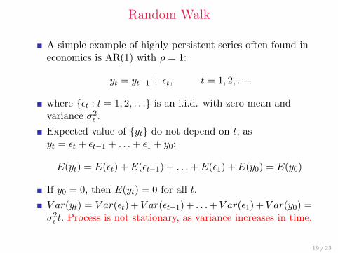
A simple example of highly persistent series often found ineconomics is AR(1) with ρ = 1:

yt = yt−1 + εt, t = 1, 2, . . .

where {εt : t = 1, 2, . . .} is an i.i.d. with zero mean andvariance σ2

ε .Expected value of {yt} do not depend on t, asyt = εt + εt−1 + . . .+ ε1 + y0:

E(yt) = E(εt) + E(εt−1) + . . .+ E(ε1) + E(y0) = E(y0)

If y0 = 0, then E(yt) = 0 for all t.V ar(yt) = V ar(εt) + V ar(εt−1) + . . .+ V ar(ε1) + V ar(y0) =σ2ε t. Process is not stationary, as variance increases in time.

19 / 23

Random Walk

Thus RW is highly persistent, as value of yt todayinfluences all the future values of yt+h:E(yt+h|yt) = yt for all h ≥ 1.Do you remember an AR(1) with ρ < 1?:E(yt+h|yt) = ρhyt for all h ≥ 1 ⇒with h→∞, E(yt+h|yt) = 0.(Ex.3): Interactive Example in Mathematica.(NOTE: To make this link work, you need to have Lecture3.cdf at the same directory

and Free CDF player installed on your computer.)

A random walk is a special case of an unit root process.

20 / 23

Random Walk

It is important to distinguish between highly persistenttime series and trending time series.Interest rate, inflation rate, unemployment rate can behighly persistent, but they do not have trend.Finally, we can have highly persistent time series withtrend: random walk with trend:

yt = α+ yt−1 + εt, t = 1, 2, . . .

where α is a drift term (see interactive Ex. 3).E(yt+h|yt) = αh+ y0.

21 / 23

Transforming Highly Persistent Time Series

Highly persistent time series can lead to very misleadingresults if CLM are violated. (do you remember spuriousregression problem?)We need to transform it into a weekly dependent process.Weakly dependent process will be referred to asintegrated of order zero, I(0).Random Walk is integrated of order one, I(1).It’s first difference is integrated of order zero, I(0):

∆yt = yt − yt−1 = εt, t = 1, 2, . . .

Therefore {∆yt} is i.i.d. sequence and we can use it foranalysis.(Ex.3.3): Interactive Example in Mathematica.

22 / 23

Thank you

Thank you very much for your attention!

23 / 23