46

Rev. Téc. Ing. Univ. Zulia. Vol. 31, Nº 3, 48 - 65, 2008

Application of the factorial design and finite element methods to optimize the solidification of Cu-5wt%Zn alloy in a sand mold

M.M. Pariona1, G.A. Salem2 and N. Cheung3

1,2Department of Mathematics and Statistics, State University of Ponta Grossa, UEPG

Campus Uvaranas, Block CIPP, Laboratory LIMAC, CEP:84030900, Ponta Grossa, PR, Brazil. mmpariona@uepg.br, moisespariona@uol.com.br

1,3Department of Materials Engineering, University of Campinas - UNICAMP, PO Box

6122, 13083-970, Campinas-SP, Brazil. cheung@fem.unicamp.br

Abstract

In the study reported in this work, two-dimensional numerical simulations were

accomplish for the solidification of the Cu-5 wt %Zn alloy in industrial greensand. The

latent heat release during the solidification using different mathematical models was

incorporated. In order to accomplish this work, the finite elements technique and the

ANSYS software program were used. The thermo-physical properties of the alloy Cu-5 wt

%Zn were considered temperature-dependent, while for sand were considered constant.

In addition, a full three-level Box-Behnken factorial design has been employed in order

to investigate the effect of the three factors on the casting process, namely initial

temperature of the mold, the convection in the external mold and the latent heat release

during the phase change. The results of the heat transfer shown throughout the 2D

system, such as thermal flow, thermal gradient and the cooling curves at various points

of the cast metal/mold were determined. It was verified that the mold temperature and

the mathematical model of the latent heat realease are the most important parameters in the solidification process.

Key words: Numerical simulation, finite elements, factorial design in three levels, solidification of alloy Cu-5wt%Zn, sand mold, latent heat release.

Aplicación de la técnica de diseño factorial y del método de elementos finitos

para optimizar la solidificación de la aleación Cu-5wt%Zn en un molde de arena

Resumen

En este trabajo fue realizada la simulación numérica en 2-D para la solidificación de la

aleación Cu-5wt%Zn en molde de arena industrial a verde. Fue incorporada en esta

investigación la liberación del calor latente durante la solidificación usando diferentes

modelos matemáticos. Para realizar este trabajo, la técnica de elementos finitos y el

software ANSYS fueron usados. Para este finalidad las propiedades termofísicas de la

aleación Cu-5wt%Zn fueron consideradas dependientes con la temperatura, entre tanto,

para la arena fueron considerados constantes. Además, el planeamiento factorial de Box-

Behnken en tres niveles fue empleado para investigar el efecto de los tres factores sobre

el proceso de la fundición, fueron entre ellos: la temperatura del molde, la convección en

la parte externa del molde y la liberación del calor latente durante el cambio de fase. Los

resultados de la transferencia de calor se presentaron en el sistema 2D para el flujo de

calor, el gradiente térmico, las curvas de enfriamiento en la pieza solidificada y en el

molde. Fue verificado que la temperatura del molde y el modelo matemático de la

liberación del calor latente durante el cambio de fase son los más importantes parámetros del proceso de la solidificación.

47

Palabras clave: Simulación numérica, elementos finitos, planeamiento factorial en tres niveles, solidificación de la aleación Cu-5wt%Zn, molde de arena, generación de calor.

Recibido el 23 de Abril de 2007 En forma revisada el 05 de Noviembre de 2008

1. Introduction

Throughout the manufacturing industry, casting process simulation has been widely

accepted as an important tool in product design and process development to improve

yield and casting quality. Casting simulation requires high-quality information concerning

thermo-physical and physical properties during solidification. Some properties have been

measured for specific alloys, but these data are generally reduced. Furthermore, the

information may be incomplete in the sense that not all properties have been measured

and sometimes, disparate information from a variety of sources is used to build up the

database for one specific alloy. In order to overcome the lack of data and achieve a

better understanding of how changes according to composition range of an alloy may

affect solidification properties, it is highly desirable to develop experimental techniques

or computer models for calculation of the thermo-physical and physical properties of multi-component alloys for the process of reliable solidification [1].

The computer simulation of cooling patterns in castings has done much to broaden our

understanding of casting and mold system design. The structural integrity of shaped

castings is closely related to the time-temperature history during solidification, and the

use of casting simulation could do much to increase this knowledge in the foundry industry [2].

The ability of heat to flow across the casting and through the interface from the casting

to the mold directly affects the evolution of solidification and plays a notable role in

determining the freezing conditions within the casting, mainly in foundry systems of high

thermal diffusivity such as chill castings. Gravity or pressure die castings, continuous

casting and squeeze castings are some of the processes where the product’s soundness

is more directly affected by heat transfer at the metal/mold interface [2].

Experimental design is a systematic, rigorous approach to solve engineering problem

that applies principles and techniques at the data collection stage so as to ensure the

generation of valid, precise, and accurate engineering conclusions [3]. It is a very

economic way of extracting the maximum amount of complex information and saving a

significant experimental time and the material used for analyses and personal costs as

well [4]. Different experimental designs are used for different objectives. For example,

randomized block designs can be used to compare data sets, and full or fractional factorial design can be used for screening relevant factors [3].

The design of experimental mixtures configures a special case of surface response

methodologies using mathematical and statistical techniques, with important applications

not only in new products design and development, but also in the improvement of the

design of existing products. In short, the methodology consists firstly to select the

appropriate mixtures from which the surface response might be calculated; and, further,

having the surface response, a prediction of the property value can be obtained for any

design, from the changes in the proportions of its components [5]. The other important

issue is for engineering experimenters who wish to find the conditions under which a

certain process attains the optimal results. In other words, it is aimed to determine the

levels of the operational factors at which the response reaches its optimum. The

optimum could be either a maximum or a minimum of a function of the design parameters [5].

48

Factorial design is a useful tool in order to characterize multivariable processes. It gives

the possibility to analyze the important influent factors of the process, and to identify

any possible interactions among them.

1.1. Mathematical solidification heat transfer model

The mathematical formulation of heat transfer to predict the temperature distribution

during solidification is based on the general equation of heat conduction in the unsteady

state, which is given in two-dimensional heat flux form for the analysis of the present study [2, 6-8].

where is density [kgm–3]; c is specific heat [J kg–1 K–1]; k is thermal conductivity [Wm–

1K–1]; ∂T/∂t is cooling rate [K s–1], T is temperature [K], t is time [s], x and y are space

coordinates [m] and Q represents the term associated to the latent heat release due to

the phase change. In this equation, it was assumed that the thermal conductivity, density, and specific heat vary with temperature.

In the current system, no external heat source was applied and the only heat generation

was due to the latent heat of solidification, L (J/kg) or DH (J/m3). Q is proportional to the

changing rate of the solidified fraction, fs, as follows [2, 6, 7].

where ∂fs ∂t is the rate of the solid fraction along the solidification.

Therefore, Eq. (2) is actually dependent on two factors: temperature and solid fraction.

The solid fraction can be a function of a number of solidification variables. But in many

systems, especially when undercooling is small, the solid fraction may be assumed as

being dependent on temperature only. Different forms have been proposed to the

relation between the solid fraction and the temperature. One of the simple forms is a linear relation [7]:

where Te and Ts are, respectively, the liquid and solid temperature (K). Scheil is another

widely used relation, which assumes uniform solute concentration in the liquid but no

diffusion in the solid [7]:

where ko the equilibrium partition coefficient of the alloy.

49

Eq. (1) defines the heat flux [9], which is released during liquid cooling, solidification and

solid cooling in classical models. The heat evolved after solidification was assumed to be

equal zero, i.e. for T<Ts, Q= 0. However, experimental investigations [9] show that

lattice defects energy, during solidification increase solid free energy, proportionally to

defects type. Lattice defects and vacancy are condensed in the already solidified part of

crystal and increase enthalpy of the solid and thus the latent heat will decrease. Due to

this fact, another way to represent the change of the solid fraction during solidification can be written as [9].

Considering c´, as pseudo specific heat, as and combining Eqs. (1) and

(2), one obtains [7, 9]

1.2. The factorial design technique

The factorial design technique is a collection of statistical and mathematical methods

that are useful for modeling and analyzing engineering problems. In this technique, the

main objective is to optimize the surface response that is influenced by various process

parameters. Surface response methodology also quantifies the relation between the

controllable input parameters and the obtained response surfaces [10]. The design procedure of surface response methodology is as follows [11]:

i. Designing a series of experiments for adequate and reliable measurement of the surface response.

ii. Developing a mathematical model of the second-order surface response with the best

fittings.

iii. Finding the optimal set of experimental parameters that produce a maximum or minimum value of response.

iv. Representing the direct and interactive effects of process parameters through two

and three-dimensional plots. If all variables are assumed to be measurable, the surface response can be expressed as follows [5]:

y= f(x1, x2, x3, …xk) (7)

where y is the answer of the system, and xi the variables of action called variables (or

factors).

The goal is to optimize the variable response y. It is assumed that the independent

variables are continuous and controllable by experiments with negligible errors. It is

required to find a suitable approximation for the true functional relation between

50

independent variables (or factors) and the surface response. Usually a second-order model is utilized in surface response methodology:

where x1, x2,…,xk are the input factors which influence the response y; bo, bii (i=1,

2,…,m), bij (i=1, 2,…,m; j=1,2,…,m) are unknown parameters and e is a random error.

The b coefficients, which should be determined in the second-order model, are obtained by the least square method.

The model based on Eq. (8), if m=3 (three variables) this equation is of the following

form:

where y is the predicted response, bo model constant; x1, x2 and x3 independent

variables; b1, b1 and b3 are linear coefficients; b12, b13 and b23 are cross product coefficients and b11, b22 and b33 are the quadratic coefficients [Kwak, 2005].

In general Eq. (8) can be written in matrix form [5].

Y=bX + e (10)

where Y is defined to be a matrix of measured values, X to be a matrix of independent

variables. The matrixes b and å consist of coefficients and errors, respectively. The solution of Eq. (10) can be obtained by the matrix approach [10; 11].

b=(X’X)–1X’Y (11)

where X’ is the transpose of the matrix X and (X’X)–1 is the inverse of the matrix X’X.

The objective of this work was to study the solidification process of the alloy Cu-5 wt

%Zn during 1.5 h of cooling. It was optimized through the factorial design in three

levels, where the considered parameters were: temperature of the mold, the convection

in the external mold and the generation of heat during the phase change. The

temperature of the mold was initially fixed in 298, 343 and 423 K, as well as the loss of

heat by convection on the external mold was fixed in 5, 70 and 150 W/m2.K. For the

heat generation, three models of the solid fraction were considered: the linear

relationship, Scheil´s equation and the equation proposed by Radovic and Lalovic [9]. As

result, the transfer of heat, thermal gradient, flow of heat in the system and the cooling

curves in different points of the system were simulated. In addition, a mathematical

model of optimization was proposed and finally an analysis by the factorial design of the considered parameters was made.

2. Methodology of the Numerical Simulation

The finite elements method was used in this study [12-15]. Software program Ansys

version 11 [16] was used to simulate the solidification of alloy Cu-5 wt %Zn in green-

sand mold. Effects due to fluid motion and contraction are not considered in the present work.

51

The geometry of the cast metal and the greensand mold is illustrated in Figure 1(a),

which is represented in three-dimensions. However, in this work the analysis was

accomplish in 2-D, which is illustrated in Figure 1(b). The material properties of a Cu-5

wt %Zn alloy were taken from the reference Miettinen [17]. In Figure 2, the phase

diagram of alloy Cu-Zn is presented [18]. An equilibrium partition coefficient of the alloy

ko=0.12 was considered in this study. Three pseudo specific heat (c´) obtained from the

equations (3), (4) and (5). These equations were denoted respectively by models A, B

and C, and the sand thermo-physical properties was given by Pariona and Mossi [19, 20].

52

In this study, the Box-Behnken factorial design in three levels [5, 21, 22] was chosen to

find out the relation between the solidification parameters. Independent variables

(factors) and their coded/actual levels were the mold temperature (x1), the convection

phenomenon (x2) and the mathematical model (x3) of the latent heat release. (Z)

represents the result of the temperature after 1.5 h of solidification. The factorial design

is shown in Table 1. For this design type a nomenclature was adopted, where for the

inferior state of the variable it was denoted by (-1), for the intermediate state by (0) and for the superior state by (+1).

53

The initial and boundary conditions were applied to geometry of the Figure 1 according

to Table 1. The boundary condition was the convection phenomenon, occurring at the

outside walls of the sand mold, as shown in Table 1. The convection coefficient at the

mold wall was considered constant in this work, due to lack of experimental data. The

effects of the refractory paint and of the gassaging process were not taken into

consideration either. The final step, consisted in solving the problem of heat transfer of

the mold/cast metal system using Equation (6) and the convergence condition was

controlled. Heat transfer is analyzed in 2-D form, as well as the heat flux and the

thermal gradient. In addition, the thermal history for some points in the cast metal and in the mold is discussed.

Table 1

Factorial design of the solidification parameters

x1

Mold

Temperature

x2

Convection

phenomenon

(hf)

x3

Mathematic

model

Z -

Temperature

after 1.5 h of

solidification

(K)

–1 298 K 5 W/m2K A

0 343 K 70 W/m2K B

+1 423 K 150 W/m2K C

1 –1 –1 –1 806.799

2 –1 –1 0 775.945

3 –1 –1 +1 862.902

4 –1 0 –1 800.301

5 –1 0 0 769.408

6 –1 0 +1 855.752

7 –1 +1 –1 798.197

8 –1 +1 0 767.562

9 –1 +1 +1 854.967

10 0 –1 –1 840.174

11 0 –1 0 809.199

12 0 –1 +1 897.176

13 0 0 –1 833.699

14 0 0 0 802.835

15 0 0 +1 890.279

16 0 +1 –1 832.200

17 0 +1 0 801.430

18 0 +1 +1 890.110

19 +1 –1 –1 899.860

20 +1 –1 0 868.171

21 +1 –1 +1 958.587

22 +1 0 –1 893.996

23 +1 0 0 862.277

24 +1 0 +1 953.026

54

25 +1 +1 –1 893.136

26 +1 +1 0 861.015

27 +1 +1 +1 952.674

3. Result and Discussion

The solidification results from the given conditions at the lines 7, 8 and 9 of Table 1,

which correspond respectively to the lowest temperatures for each mathematical model

of latent heat release, were discussed. Each one of the lines corresponds to the

temperature of the mold for the lower state (-) and for convection phenomenon for the higher state (+).

The condition mentioned on line 9 of Table 1 was chosen to present heat transfer results,

where the temperature field is shown in Figure 3(a) in all the system mold and in the

cast metal (Figure 3(b)). This last case can be visualized in more detail in part (b),

where an almost uniform temperature is observed. In the geometric structure of the

mold there is a core constituted of sand that is represented by a white circle in Figure

3(b), which can be verified also in Figure 1(a). In Figure 4 the results of the thermal

gradient and the thermal flux are shown, where the thermal gradient goes from the cold

zone to the hot zone. On the other hand, the thermal flux goes from the hot zone to the

cold zone. Also the convergence of the solution was studied; this point is discussed in more detail by Pariona and Mossi [19, 20].

55

56

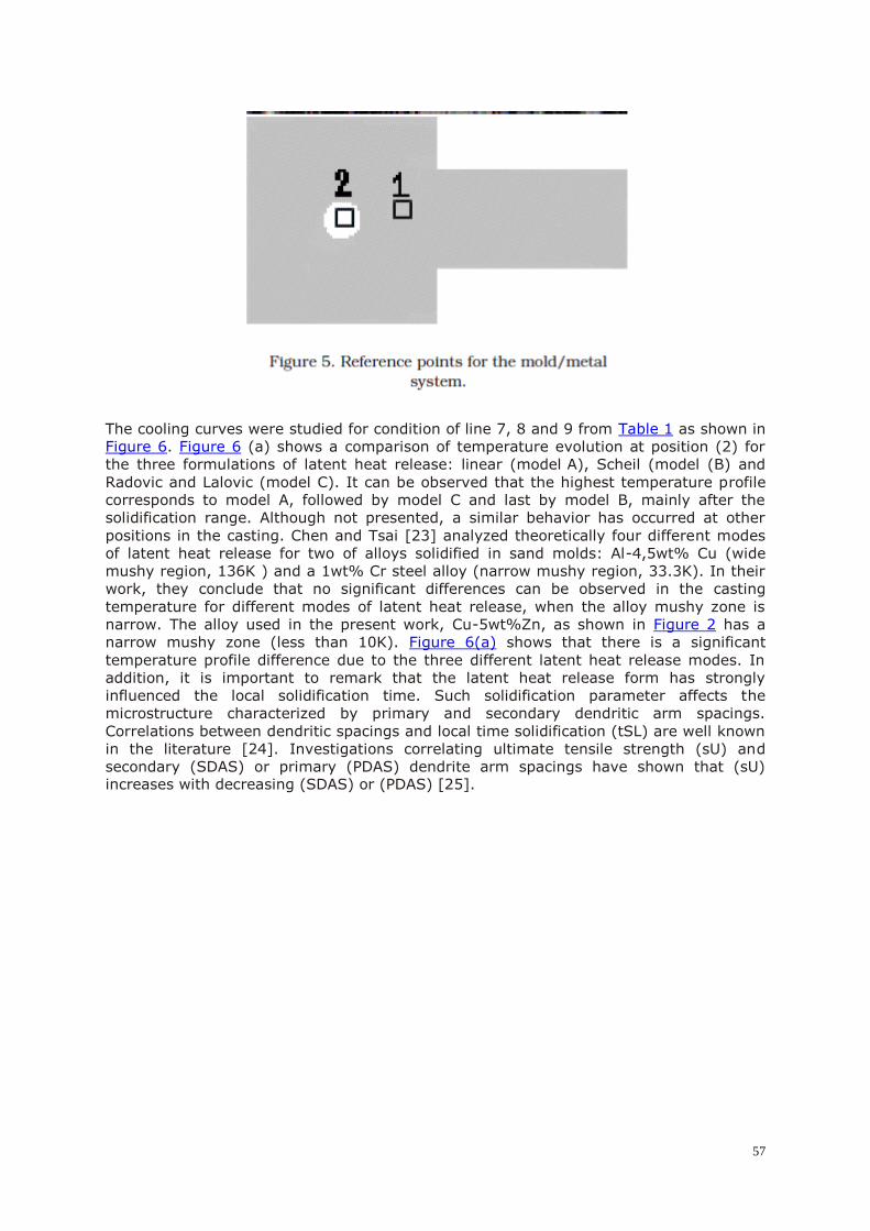
In order to simulate the cooling curves, two points were considered, as shown in Figure

5: one located in the core (2 point) and the other in the metal (1 point). The three forms

of latent heat release were applied into the mathematical model and the resulting thermal profiles were compared.

57

The cooling curves were studied for condition of line 7, 8 and 9 from Table 1 as shown in

Figure 6. Figure 6 (a) shows a comparison of temperature evolution at position (2) for

the three formulations of latent heat release: linear (model A), Scheil (model (B) and

Radovic and Lalovic (model C). It can be observed that the highest temperature profile

corresponds to model A, followed by model C and last by model B, mainly after the

solidification range. Although not presented, a similar behavior has occurred at other

positions in the casting. Chen and Tsai [23] analyzed theoretically four different modes

of latent heat release for two of alloys solidified in sand molds: Al-4,5wt% Cu (wide

mushy region, 136K ) and a 1wt% Cr steel alloy (narrow mushy region, 33.3K). In their

work, they conclude that no significant differences can be observed in the casting

temperature for different modes of latent heat release, when the alloy mushy zone is

narrow. The alloy used in the present work, Cu-5wt%Zn, as shown in Figure 2 has a

narrow mushy zone (less than 10K). Figure 6(a) shows that there is a significant

temperature profile difference due to the three different latent heat release modes. In

addition, it is important to remark that the latent heat release form has strongly

influenced the local solidification time. Such solidification parameter affects the

microstructure characterized by primary and secondary dendritic arm spacings.

Correlations between dendritic spacings and local time solidification (tSL) are well known

in the literature [24]. Investigations correlating ultimate tensile strength (sU) and

secondary (SDAS) or primary (PDAS) dendrite arm spacings have shown that (sU) increases with decreasing (SDAS) or (PDAS) [25].

58

59

Figure 6 (b) shows a comparison of temperature evolution at position (4) for the three

formulations of latent heat release. It can be observed again, that the highest

temperature profile corresponds to model A, followed by model C and last by model B, and this behavior is repeated for the other positions in the mold.

A three level Box-Behnken design [5, 21, 22] was used to determine the responses of

the three variables x1, x2 and x3, basing in Table 1. The result of this analysis is shown in

the Pareto’s diagram (Figure 7). In this figure the estimated valor of the result Z is

presented with the significance level (p) of 95%, showing the variables with and without

influences significant. The notation adopted for this analysis was, “L” means linear, “Q”

means quadratic. For example, “(1)” is the main effect of the first factor and “2L by 3Q”

means the linear interaction of the parameter 2 (convection phenomenon) with the

quadratic effect of parameter 3 (latent heat release form). In Figure 7, two significant

influences were found: x1 (mold temperature) with linear effect and x3 (mathematical

model) with linear and quadratic effects. The other effect of the independent variables

and interactions are negligible in this figure. In order to understand better this analysis,

other type of standard graph was accomplished, and it is shown in Figure 8. This figure

of the factorial design was built based on the Student’s probability distribution (t) [22].

In this figure the main effects and their interactions with significant influence can be

observed by those dispersed points (around of the straight line). Those points that

belong to the concentrated region points are of the negligible influence. It can be

observed in Figure 8 that the biggest positive influence is due to the main effect of x1

(mold initial temperature) with linear behavior, followed by the linear and quadratic

effect of parameter 3 (latent heat release form). Parameter x2 with linear behavior

presents a small negative influence on the factorial design and the other effects had a

negligible behavior, around zero, as presented in Figure 8. For this analysis a

mathematical model was proposed, given by the following equation Z:

60

61

In this equation the linear and quadratic coefficients are the most important parameters

and the other coefficients are negligible (they are considered as residue). Precisely the

most significant coefficients belong to the variables which strongly influence the result, as it can be observed in Figures 7 and 8.

Figure 9 presents the surface response plots [5, 21], obtained from Eq. (12), that

describe the influence of the factors on the overall desirability. Fig. 9(a) shows the 3D

surface response relation between convection phenomenon (x2) and latent heat release

form (x3) at zero level of mold temperature (x1). Note that, for a given value of x2, as

the x3 increases and the Z decreases until a minimum value for the interval of x3

between -0.8 and 0.2. After this minimum point, Z changes its behavior and start to

increase as the x3 increases reaching the highest value of 958.587, as can be seen in

Table 1. For a given value of x3, it can be observed that z profile is almost constant in

relation to x2 increase. Another way to visualize Z variation, is to project Z on the x2 and

x3 plane in terms of grayscale. The region limited by the white points on this curve

represents the Z confidence interval. For other levels of x1, the surface graph behavior has same characteristic as previously mentioned.

62

63

Fig 9(b) shows the effect of mold temperature (x1) and latent heat release form (x3) at

zero level of convection phenomenon (x2). In this case, x1 e x3 generated a complex

surface of paraboloid type. According to the surface projection on the x1 and x3 plane, for

a given x3 value, it can be observed that the variation of Z is linear in relation to x1 and

this fact can be confirmed by the point x1(L) mentioned at the graph Figure 8. On the

other hand, the same cannot be affirmed in relation to x3, if the same analysis is done.

For a given value of x1, the variation of z is parabolic in relation to x3 and this fact can be observed by the points x3(L) and x3(Q) mentioned at the graph of Figure 8.

Fig 9(c) shows the effect of mold temperature (x1) and convection phenomenon (x2) at

zero level of latent heat release (x3). Note that, as the x1 factor increases, the Z

increases. But, for a given value of x1, it is observed that for every x2 value, Z is almost

constant. As a result, the surface geometry is not a complex one, if we compare to the surface geometry of Figure 9b.

In this type of analysis, one can realize that the parameters x1 and x3 had variations

more accentuated than the parameter x2. This behavior is also verified in the Figures 7 and 8.

4. Conclusion

The three latent heat release forms implemented into the model resulted in significant

different thermal responses, which contradicts a previous report in the literature.

In this study, a three-level Box-Behnken factorial design combining with a surface

response methodology was employed for modeling and optimizing three operations

parameters of the casting process. According to this study, it was observed that the

parameters, such as, mold temperature and the mathematical model of the latent heat

realease are the most important in the solidification process. The factorial design method

is a useful tool to determine what factors are crucial in the solidification process and thus, a special care needs to be taken during the project elaboration of the casting.

5. Acknowledgements

The authors acknowledge financial support provided by CNPq (The Brazilian Research Council).

6. References

1. Guo Z., Saunders N., Miodownik A.P. and Schillé J.-Ph. “Modelling of materials

properties and behaviour critical to casting simulation”. Materials Science and

Engineering, A 413-414: (2005). 465-469.

2. Ferreira I.L., Spinelli J.E., Pires J.C. and Garcia A. “The effect of melt temperature

profile on the transient metal/mold heat transfer coefficient during solidification”.

Materials Science and Engineering, A 408: (2005). 317-325.

3. Xiao Z., Vien A. “Experimental designs for precise parameter estimation for non-linear

models” . Minerals Engineering, 17: (2004). 431-436.

4. Kincl M., Turk S., Vrecer F. “ Application of experimental design methodology in

development and optimization of drug release method. International Journal of

Pharmaceutics” , 291: (2005). 39-49.

64

5. Aslan N. “Modeling and optimization of Multi-Gravity Separator to produce celestite

concentrate”. Powder Technology, 174: (2007). 127-133.

6. Santos CA., Fortaleza EL., Ferreira CRF., Spim JA. and Garcia A. “A solidification heat

transfer model and a neural network based algorithm applied to the continuous casting

of steel billets and blooms”. Modelling Simul Mater Sci Eng, 13: (2005). 1071-1087.

7. Shi Z. and Guo Z.X. “Numerical heat transfer modelling for wire casting” . Materials

Science and Engineering, A365: (2004). 311-317.

8. Dassau E., Grosman B. and Lewin D.L. “Modeling and temperature control of rapid

thermal processing”. Computers and Chemical Engineering, 30: (2006). 686-697.

9. Radovic Z. and Lalovic M. “Numerical simulation of steel ingot solidification process” .

Journal of Materials Processing Technology, 160: (2005). 156-159.

10. Kwak J.S. “Application of Taguchi and response surface methodologies for geometric

error in surface grinding process”. International Journal of Machine Tools and

Manufacture, 45: (2005). 327-334.

11. Gunaraj V., Murugan N. “Application of response surface methodologies for

predicting weld base quality in submerged arc welding of pipes”. Journal of Materials

Processing Technology, 88: (1999). 266-275.

12. Su X. “Computer aided optimization of an investment bi-metal casting process”.

Ph.D. Thesis, University of Cincinnati, Department of Mechanical, Industrial and Nuclear

Engineering. Cincinnati, 2001.

13. Shi Z. and Guo Z.X. “Numerical heat transfer modelling for wire casting”. Materials

Science and Engineering, A365: (2004). 311-317.

14. Janik M. and Dyja H. “Modelling of three-dimensional temperature field inside the

mould during continuous casting of steel”. Journal of Materials Processing Technology,

157-158: (2004). 177-182.

15. Grozdanic´ V. “Numerical simulation of the solidification of a steel rail-wheel casting

and the optimum dimension of the riser” . Materiali in tehnologije, 36: (2002). 39-41.

16. Handbook Ansys, Inc, Canonsburg, PA, 2007.

17. Miettinen J. “Thermodynamic-Kinetic simulation of solidification in binary fcc copper

alloys with calculation of thermophysical properties”. Computational Materials Science,

22: (2001). 240-260.

18. Thermo-Calc Software, Stockholm, Sweden, 2007.

19. Pariona M.M. and Mossi A.C. “Numerical Simulation of Heat Transfer During the

Solidification of Pure Iron in Sand and Mullite Molds” . J of the Braz Soc of Mech Sci &

Eng, XXVII: (2005). 399-406.

65

20. Pariona M.M. and Mossi A.C. “Numeric simulation of the solidification of the pure iron

varying the solidification process parameters”. Rev Téc Ing Univ Zulia, 29: (2006). 197-

208.

21. Paterakis P.G., Korakianiti E.S., Dallas P.P, Rekkas, D.M. “Evaluation and

simultaneous optimization of some pellets characteristics using a 33 factorial design and

the desirability function”. International Journal of Pharmaceutics, 248: (2002). 51-60.

22. Montgomery C.D. “Design and Analysis of Experiments”, John Wiley & Sons, New

York, 1999.

23. Chen J.H., Tsai H.L. “Comparison on different modes of latent heat release for

modeling casting solidification”, AFS Transactions, (1990) 539-546.

24. Garcia, A, “Solidificação - Fundamentos e Aplicações”. Editora da Unicamp, Campinas

- SP, 2007.

25. Quaresma, J.M.V., Santos, C.A., Garcia, A. “Correlation between unsteady-state

solidification conditions, dendrite spacings, and mechanical properties of Al-Cu alloys”.

Metallurgical and Materials Transactions A, 31A: (2000). 3167-3177.