Application of Pulse Response Extraction to Nonlinear Data ... · Application of Pulse Response Extraction to Nonlinear Data Channels 4 The pulse response analysis methods described

DesignCon 2017

Application of Pulse Response Extraction to Nonlinear Data Channels

Richard Allred, [email protected]

Michael Steinberger, [email protected]

Todd Westerhoff, [email protected]

DesignCon 2017 1

ABSTRACT

Even when the waveform source is nonlinear, it is possible to extract an apparent pulse response from a time domain data waveform. While such a pulse response's mathematical properties are limited, it can still be used to provide accurate BER estimates through statis-tical analysis, and offers other insights through pulse response analysis. This paper reviews two known methods for pulse response extraction and, through comparison to time domain simulation results for both NRZ and PAM4 modulations, presents some pos-sibilities and limitations of this approach in the analysis of nonlinear data channels.

Author(s) Biography

Richard AllredRichard Allred has nearly a decade of experience in cutting edge signal integrity. After receiving his Masters degree from the University of Utah, he joined Intel in Oregon where he worked on the Larrabee GPU project and lead the memory interface KIT. Next he joined Inphi, where he contributed to the industry's first CMOS 28G VSR / 100G Ethernet PHY. In 2013 he joined SiSoft where he now focuses on IBIS-AMI modeling and tool development. He is the author of several DesignCon papers, has a patent pending and is pursuing a Ph.D. at the University of Utah. When not working, he enjoys spending time with his family and getting out of cell-phone range in the mountains and deserts of the western US.

Michael SteinbergerMichael Steinberger, Ph.D., Lead Architect for SiSoft, has over 30 years' experience designing very high speed electronic circuits. Dr. Steinberger holds a Ph.D. from the Uni-versity of Southern California and has been awarded 14 patents. He is currently responsi-ble for the architecture of SiSoft's Quantum Channel Designer tool for high speed serial channel analysis. Before joining SiSoft, Dr. Steinberger led a group at Cray, Inc. perform-ing SerDes design, high speed channel analysis, PCB design and custom RAM design.

Todd WesterhoffTodd Westerhoff, VP Semiconductor Relations at SiSoft, has over 37 years of experience in modeling and simulation, including 20 years of signal integrity experience. He is responsible for SiSoft's activities working with semiconductor vendors to develop high-quality simulation models. Todd has been heavily involved with the IBIS-AMI modeling specification since its inception. He has held senior technical and management positions for Cisco and Cadence and worked as an independent signal integrity consultant. Todd holds a B.E.E.E. degree from the Stevens Institute of Technology in Hoboken, New Jer-sey.

Application of Pulse Response Extraction to Nonlinear Data Channels 2

1.0 Overview

This paper offers an engineering approach to the analysis and performance estimation of nonlinear high speed serial channels. While there are rigorous mathematical approaches to the analysis and performance estimation of linear, time invariant (LTI) high speed serial channels, the mathematics breaks down when the LTI assumption is violated. The other generic approach is time domain simulation; however, it is impractical to achieve signifi-cant statistical coverage for the bit error rates typically required from high speed serial channels.

The approach in this paper is an engineering approach in the sense that it depends on an approximation for which we can offer no rigorous mathematical proof. That is, we assume that a pulse response can be a useful characterization of a serial channel even if that pulse response was derived from the time domain waveform of a nonlinear channel. As is the case with all approximations, there are limits to both the accuracy and application of this approximation. Nonetheless, it can be a very useful engineering tool so long as the engi-neer considers these limitations when making design decisions.

1.1 Applications and Limitation

This paper addresses only intersymbol interference as an impairment, as there are known techniques for introducing other impairments such as noise, jitter and crosstalk once the intersymbol interference has been evaluated. For intersymbol interference on nonlinear serial channels, we consider two primary problems:

1. Design/evaluation of channel equalization

2. Bit error rate estimation for low error rates

Channel Equalization: For an LTI channel, one can obtain a pulse response by convolving an ideal pulse with the appropriate impulse response. If the impulse response is for the combination of transmit equalizer, channel, and receive equalizer, there are straightfor-ward visual techniques for understanding the effectiveness of the equalization and the trade-offs between the different equalization mechanisms available [1]. However, the impulse response is not defined for a nonlinear channel and so a pulse response cannot be produced through the linear convolution method.

BER Estimation: While statistical analysis is a very effective method for estimating the bit error rate at low error rates, it also depends on the LTI assumption and is therefore not directly applicable to nonlinear channels. The other option is time domain simulation. However, as will be demonstrated in a later section, it simply isn’t practical to run a time domain simulation long enough to achieve statistically significant data for a low error rate.

By defining an alternate approach to calculating a pulse response, this paper introduces new options for addressing these two problems. We will use the term “pseudo-pulse response” to indicate that the response is not necessarily the response of an LTI channel, and therefore does not have the same mathematical properties as the pulse response of an LTI channel.


The pulse response analysis methods described in [1] can be applied directly to pseudo-pulse responses, and the analysis of such a waveform will produce equally useful engi-neering insights into channel equalization. Furthermore, statistical analysis based on pulse responses produced by this alternate approach generates reliable results for low error rates.

Pseudo-pulse responses do have their limitations, however. One particularly visible limita-tion is that a step response generated using a pseudo-pulse response has no useful applica-tion that we’ve been able to find. This comment applies especially to statistical analysis based on step responses rather than pulse responses- it simply doesn’t work when the pulse response was derived using this alternate approach.

1.2 Pulse Response Calculation Methods

The pulse response calculation methods presented in this paper extract an equivalent pulse response from a time domain simulation. The steps are

1. Run the time domain simulation long enough that the system reaches a steady state. While we do present an approach for handling relatively small violations of time invari-ance, the system must first converge to its steady state operating range.

2. Run a predetermined repeating data pattern through the system and accumulate a time domain waveform at the output of the system for one complete repetition of that data pattern.Time variance: In the case of a channel with a small amount of time variation, it may be helpful to accumulate the average from several iterations of the repeating data pat-tern.

3. Use either Hilbert space projection or the inversion of a circulant matrix to extract an equivalent pulse response from the time domain waveform at the output of the system. Both of these methods are relatively simple to implement, are computationally very efficient, and yield equivalent results.

This approach has the advantage that it can be applied to time domain waveforms from either LTI or nonlinear systems. For an LTI system, the pulse response is exactly the same as that obtained using linear convolution. For even a highly nonlinear system, the resulting pulse response can still be recognized as a pulse response.

From a mathematical perspective, there are two main limitations:

1. The results are very much dependent on the data pattern chosen. The characteristics of the autocorrelation of the data pattern are visible in the resulting pulse response. We have gotten good results with linear feedback shift register sequences, also call pseudo-random bit sequences (PRBS), although we have found PRBS7 to be too short to pro-duce good results.

2. Both pulse response extraction techniques involve the inversion of a linear operator, and are therefore subject to small variations at frequencies for which the spectral den-sity of the time domain waveform is low. For a nonlinear system and a repeating data pattern, there will always be such frequencies, especially at frequencies equal to an


integer multiple of the data rate. The numerical artifacts due to these frequencies are readily visible in either the time or frequency domain.

1.3 Approximation Characterization

Since what this paper offers is an engineering approximation, any results are at best dem-onstrations of the degree to which the approximation is effective in one or more specific cases, and cannot be generalized beyond the data presented. We can only state that in our experience in many analyses performed over the last eight years, this approximation has proven to produce useful results.

In order to understand the accuracy limitations of pseudo-pulse responses, results are com-pared to time domain simulation results for varying amounts of nonlinearity in the chan-nel.

For the channel equalization analysis application, we will compare the linear pulse with the pulse response computed for the different amounts of channel nonlinearity. The chan-nel and equalization were chosen specifically to make the effects of nonlinearity clearly visible for the NRZ modulation. It will be seen that although there are clearly visible arti-facts due to the nonlinearity, those artifacts tend to be at bit boundaries rather than near the bit sampling time, and therefore do not affect the accuracy of the engineering analysis.

For the statistical analysis applications, we will compare the bathtub curve predicted by the statistical analysis of a pseudo-pulse response to the bathtub curve produced through time domain simulation. The underlying assumption is that although time domain simula-tion may have its limitations, it does at least accurately model the nonlinearities and time variations, and so is the most reliable baseline available.

This comparison between statistical analysis and time domain simulation must, however, account for the uncertainty associated with the finite duration of the time domain simula-tion. For a given decision timing offset, the accuracy of the error rate estimate becomes very poor when the number of detected error events is small. We will present the simple equations that describe the accuracy of time domain simulations and show this inaccuracy explicitly when comparing results. The net result is that even for very long time domain simulations, a useful comparison can still only be made for error rates that are many orders of magnitude higher than the error rate required for most high speed serial channels. The associated engineering assumption is that if statistical analysis of a pseudo-pulse response matches time domain simulation within the error limits of the time domain simulation, then it’s as reliable a prediction as we can find for lower error rates.

1.4 PAM4

While the first approximation characterizations will be for NRZ modulation, we do also apply pseudo-pulse analysis to channels with PAM4 modulation. However, in a PAM4 eye, the outer eyes can have a smaller eye height than the inner eye. We model this com-pression of the outer eyes as being due to gain compression, resulting in a lower amplitude for the outer symbols than would be predicted by linear analysis.


In order to get useful results, we’ve found it necessary to modify the statistical analysis method by hypothesizing an amplitude compression factor for the outer symbols. This amplitude compression factor is derived from the PAM4 waveform, and we will show results vs. saturation level in the same way we do for NRZ.

2.0 Accuracy of Time Domain Simulations

2.1 BER Standard Deviation Calculation

Consider for the sake of specificity a time domain simulation in which the data bits at the output of the receiver decision circuit are compared directly to a time shifted version of the uncorrelated (“random”) data used to drive the transmitter. That is, the time shift is chosen in such a way that the data at the output of the receiver match the time shifted transmit bits most of the time. Following some settling time for the simulation, the mis-matches are counted- producing an error count for the simulation.

Suppose, furthermore, that this bit comparison and error counting is performed both for the decision clock at the timing produced by the receiver’s clock recovery circuit and for decision clock timings offset from the recovered clock timing. The result will be a curve of error count vs. receiver clock offset. Suppose that the clock offset has been varied from negative one half of the symbol time to one half of the symbol time. Then the error counts can be expressed as a function . If the total number of bits simulated after

the settling time of the simulation is , then the estimated error rate vs. clock offset is

(EQ 1)

and the plot of vs. is called a bathtub curve because the estimated error rate tends to be approximately one half for timing offsets at the ends of the range but falls to a low value in the center of the range.

Recognize, however, that a bathtub curve derived in this way can only be an estimate because there was only a finite number of bits in the simulation. Even if the transmit data was truly random, the simulation was only a finite sample of a statistical process.

If we adopt the assumption that the individual bit errors for a given clock offset are statis-tically independent events, then we can use the same mathematics that Physicists use for event counting experiments [2]- namely that the variance of the measurement is equal to the square root of the average number of events counted. This is often approximated as the square root of the number of events actually counted. For the time domain simulation experiment, the resulting equation for the standard deviation of the error rate estimate is

(EQ 2)

τo

Ne τo( )

Nt

perr τo( )Ne τo( )

Nt----------------=

perr τo( ) τo

σ τo( )Ne τo( )

Nt--------------------=


For bit errors due to intersymbol interference, the assumption that the individual error events are independent is actually optimistic, especially at higher error rates. As demon-strated by some data presented at an FEC tutorial [3], errors due to intersymbol interfer-ence tend to cluster, although not because of DFE error propagation. Rather, it appears that the intersymbol interference from several timing offsets can combine multiple times to produce errors that are relatively close together. At one company that studied these phe-nomena extensively, they came to attribute these error clusters to “killer packets”.

If, as seems to be the case, bit errors due to intersymbol interference are not quite statisti-cally independent, then the number of statistically independent events is actually lower than the number of bit errors. If the average size of a statistically independent error event is , then Equation 2 becomes

(EQ 3)

For the work reported in this paper, we have chosen not to pursue the subject of error clus-tering, and so will use Equation 2 as an optimistic lower bound for the standard deviation of the error rate estimate.

Another problem occurs when there have been no error events in the simulation for a given clock offset. The fact that no errors were counted does not necessarily mean that the error rate at that clock offset is identically zero. All it means is that the error rate is at least somewhat lower than the resolution of the simulation. In this case, we cannot adopt the approximation that the average number of errors counted is equal to the number of errors actually counted, and so Equation 2 is not a valid approximation. In this case we will iden-tify a error rate floor based on the length of the simulation

(EQ 4)

Confidence Limits: As a further approximation, we assume that the probability density function at a given clock timing approximates a Gaussian function. The 90% confidence limits are then at

(EQ 5)

2.2 Time Domain Simulation Accuracy Demonstration

To demonstrate the mathematics of the previous section, statistical analysis and two time domain simulations were run for a perfectly LTI channel. One of the time domain simula-tions was for a million bits while the other was for 300 million bits. In this section, we will compute the standard deviation for the two different lengths of time domain simulation, and we will compare the results to the results from statistical analysis. Note that since the channel is LTI, the pseudo-pulse response is all but identical to the pulse response com-

a

σ τo( )a

Ne τo( )a

----------------

Nt------------------------ a

Ne τo( )Nt

--------------------= =

σmin1Nt-----=

perr τo( ) 1.6σ τo( )±


puted through linear convolution; and so the results obtained from statistical analysis would be all but identical as well.

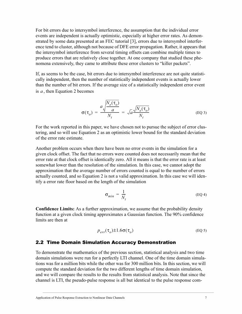
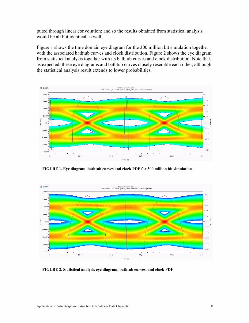
Figure 1 shows the time domain eye diagram for the 300 million bit simulation together with the associated bathtub curves and clock distribution. Figure 2 shows the eye diagram from statistical analysis together with its bathtub curves and clock distribution. Note that, as expected, these eye diagrams and bathtub curves closely resemble each other, although the statistical analysis result extends to lower probabilities.

FIGURE 1. Eye diagram, bathtub curves and clock PDF for 300 million bit simulation

FIGURE 2. Statistical analysis eye diagram, bathtub curves, and clock PDF


Figure 3 is a comparison between the eye diagram contours for the 300 million bit simula-tion and the statistical analysis. Contours are shown for the probabilities 10-3, 10-6, and 10-9. These contours are included primarily as a baseline for later contour comparisons.

FIGURE 3. Eye contour comparison: 300 million bit time domain (blue) vs. statistical analysis (red). Contours at 10-3, 10-6 and 10-9.

Figure 4 and Figure 5 compare the bathtub curves for the one million bit simulation, the 300 million bit simulation and the statistical analysis. The one million bit error rate esti-mate and its upper and lower 90% confidence limits are shown in red. The 300 million bit error rate estimate and its upper and lower limits are shown in green, and the statistical analysis result is shown in blue. Figure 4 shows all of the data while Figure 5 is a more detailed view of the most important data.

FIGURE 4. Bathtub curve comparison between one million bit simulation, 300 million bit simulation, and statistical analysis


Note how the data remains consistent with the upper and lower confidence limits, and how the error rate resolution increases going from the one million bit simulation to the 300 mil-lion bit simulation to the statistical analysis. Note also that even the 300 million bit simu-lation provides no useful information about the clock offsets that might produce a 10-12 error rate, whereas the statistical analysis does.

FIGURE 5. Detailed view of bathtub curve comparison

3.0 Pulse Response Extraction

The problem to be solved is: Given a repeating data pattern and a repeating sampled time domain waveform generated from that data pattern, compute a pulse response

which could have produced the waveform from the data pattern.

Given , data sequence length and samples per symbol , one can represent the data pattern as a sequence of impulses

(EQ 6)

The desired result is that

(EQ 7)

where is the circular convolution operator for waveforms of length .

While the goal of the Hilbert space projection is to create a pulse response which produces a least square error approximation to the time domain waveform, the circulant matrix approach demonstrates that the solution is exact. The two approaches solve the same equa-tion and therefore produce the same result. The Hilbert space projection approach is most

d n[ ]w m[ ]

p m[ ]

d n[ ] N M

u m[ ] d k[ ]δ m kM–( )k 0=

N 1–

∑=

w m[ ] u m[ ] p m[ ]⊗=

NM


efficient computationally for PRBS patterns while the circulant matrix approach maintains its computational efficiency over a wide range of data patterns.

3.1 Hilbert Space Projection Approach

Hilbert space projection approximates a target vector as the linear combination of a set of vectors called basis vectors. The basis vectors form a subspace of the Hilbert space. Every vector in the subspace is a linear combination of the basis vectors and every linear combi-nation of basis vectors is a member of the subspace. The target vector is a member of the Hilbert space but usually not a member of the subspace and so there usually isn’t an exact match.

In the case of pulse extraction, the set of basis vectors is the set of all

circularly shifted versions of the impulse sequence . That is,

(EQ 8)

Note that there is a basis vector for every sample position in the waveform.

A Hilbert space also has an inner product that produces a real or complex number from two vectors in the space. For this problem the inner product is simply the usual vector inner product

(EQ 9)

The approximation is then calculated (Gram-Schmidt procedure) by first calculating a vector of inner products with the target

(EQ 10)

and a matrix of inner products of the basis vectors with each other, called the Gram matrix:

(EQ 11)

The so-called “normal equation” is the vector equation

(EQ 12)

where is a column vector containing the samples of the desired pulse response. The solution is therefore

(EQ 13)

bk{ } 0 k N<≤

u m[ ]

bk m[ ] u m[ ] δ m k–( )⊗≡

x m[ ] y m[ ]• x n[ ] y n[ ]⋅n 0=

NM

∑≡

α

α k[ ] bk m[ ] w m[ ]•=

G

G i j,[ ] bi m[ ] bj m[ ]•≡

Gp α=

p

p G 1– α=


The desired pulse response is then read directly from the vector .

3.2 Circulant Matrix Approach

The circulant matrix approach casts Equation 7 as a matrix equation

(EQ 14)

where is a column vector containing the samples of the target waveform, is a matrix in which each row is a circularly shifted version of as in Equation 8 and is a col-umn vector containing the samples of the desired pulse response.

The equation is solved by inverting the matrix . Since each row is a circularly shifted version of the row above it, the matrix is called a circulant matrix. Such a matrix can be inverted very efficiently [4] using essentially Fourier transform techniques. (Another way to look at this is that Equation 7 can easily be transformed to the frequency domain, solved in the frequency domain and then transformed back to the time domain; however, try to avoid dividing by small numbers.)

A future paper by Richard Allred will expand on this approach in a number of ways.

4.0 Equalization Characterization Results

To make the effects of nonlinearity on NRZ modulation as clearly visible as possible, we designed a relatively low loss channel with a comparatively large amount of ringing due to multiple reflections, as shown in Figure 6. Since the channel loss is abnormally low, a lumped model was used for one of the transmission lines in order to reduce the numerical artifacts at high frequencies. It is a poor design for performance but within our range of experience from studies of real systems [5]. This channel was combined with a receiver consisting of a saturating nonlinearity and DFE equalization. Since the channel loss was so low, no transmit equalization was required.

FIGURE 6. Demonstration channel for NRZ modulation

The goal of this demonstration design is to get the nonlinearity to affect a linear equalizer. Since a saturating nonlinearity insert between the final stage of equalization and the deci-

p m[ ] p

w Up=

w Uu m[ ] p

U


sion point will have very little effect on the resulting error rate, the linear equalizer must be inserted between the saturating nonlinearity and the receiver decision point. That’s DFE.

The four receiver saturation curves are shown in Figure 7. Y0 is completely linear up to a saturation voltage of volts, while the saturation curves Y1 through Y3 introduce increasing degrees of saturation. The primary difference between Y2 and Y3 is that Y3 is a rounder curve that starts introducing nonlinear distortion at lower amplitudes.

The receiver’s DFE has five taps and uses the typical zero-forcing algorithm to choose its tap values.

FIGURE 7. Demonstration saturation curves

The Hilbert space projection approach of Section 3.1 using a PRBS11 pattern was applied to the demonstration channel described above. Figure 8 is a plot of the resulting pseudo-pulse responses for each of the saturation curves. In this figure and the subsequent two fig-ures, the time scale has been set to unit intervals (UI) instead of seconds, the response baselines are set to zero volts, and the response has been shifted in time so that the clock time that would recovered from the response is set to zero. This clock recovery was per-formed using the “hula hoop” algorithm described in [1]. Figure 8 is presented as a com-plete view of the data; however, it doesn’t show very much.

Figure 9 is a magnified view that would typically be used to analyze equalization behav-ior. In this figure, the time alignment, time scale, and response baseline make it easier to understand the equalization behavior. The main pulse is at time zero and the response val-ues at integer multiples of one UI are the intersymbol interference contributors from adja-cent symbols.

In Figure 9, the intersymbol interference contributors for the first five adjacent symbols are zero, demonstrating that the DFE taps are performing as expected, even with the pres-ence of the saturating nonlinearity. Figure 9 also shows that as the degree of nonlinearity

0.5±


is increased, the amplitude of the main pulse gets smaller. This was also expected. Thus, at least for this demonstration project, the pseudo-pulse response seems to be useful for the analysis of channel equalization behavior in the sense that it illustrates the behavior we expect for a case we understand.

FIGURE 8. Pseudo-pulse responses vs. Nonlinearity

FIGURE 9. Pseudo-pulse responses for analyzing equalization behavior


Figure 10 is a magnified view of the artifacts in a pseudo-pulse response. These artifacts are very short in duration and not particularly large in amplitude; but they persist across the entire time space of the response. We have experimented with removing these artifacts and have found that in fact they are absolutely required to get results from statistical anal-ysis that match time domain simulation results. Without these artifacts, the statistical anal-ysis results are significantly optimistic.

The pseudo-pulse artifacts become a dominant feature when a step response is calculated from a sequence of pseudo-pulse responses, as shown in Figure 11. Using the variable def-initions from Section 3.0, the step response is calculated as

(EQ 15)

When a step response is calculated from a linear pulse response, the value of the pulse response decays to zero and stays there; so the baseline value from previous pulse responses in the calculation have minimal effect on the steady state value of the step. However for the pseudo-pulse response, the sum continues to grow. There is even a little of this phenomenon for the Y0 saturation curve because it saturates at and there were a few samples in the waveform that had a greater magnitude than that.

FIGURE 10. Magnified view of pseudo-pulse response artifacts

s m[ ] p m kM–[ ]k 0=

m kM 0≥–

∑=

0.5±


FIGURE 11. Step responses produced from pseudo-pulse responses

Figure 12 is a magnified view of the step responses. In this view, it appears that the arti-facts end up forming a ripple that has a period equal to one UI. This is an illustration of the linear operator inversion numerical processing limitation mentioned in Section 1.2. The repeating data waveform driving the channel has very low spectral density at frequencies close to integer multiples of the data rate; however the nonlinear response of the channel tends to cause these spectral nulls to become shallower in the output waveform. In essence, the output spectral density is divided by the input spectral density. This is particu-larly clear for the circulant matrix approach described in Section 3.2. (Remember that comment about trying to avoid dividing by small numbers?) This division of one spectral density by another produces very large peaks in the spectral density of the pseudo-pulse response at frequencies which are an integer multiple of the data rate.

FIGURE 12. Magnified view of step responses produced by pseudo-pulse responses


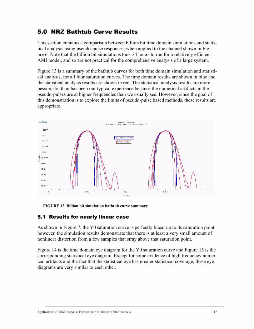
5.0 NRZ Bathtub Curve Results

This section contains a comparison between billion bit time domain simulations and statis-tical analysis using pseudo-pulse responses, when applied to the channel shown in Fig-ure 6. Note that the billion bit simulations took 24 hours to run for a relatively efficient AMI model, and so are not practical for the comprehensive analysis of a large system.

Figure 13 is a summary of the bathtub curves for both time domain simulation and statisti-cal analysis, for all four saturation curves. The time domain results are shown in blue and the statistical analysis results are shown in red. The statistical analysis results are more pessimistic than has been our typical experience because the numerical artifacts in the pseudo-pulses are at higher frequencies than we usually see. However, since the goal of this demonstration is to explore the limits of pseudo-pulse based methods, these results are appropriate.

FIGURE 13. Billion bit simulation bathtub curve summary

5.1 Results for nearly linear case

As shown in Figure 7, the Y0 saturation curve is perfectly linear up to its saturation point; however, the simulation results demonstrate that there is at least a very small amount of nonlinear distortion from a few samples that stray above that saturation point.

Figure 14 is the time domain eye diagram for the Y0 saturation curve and Figure 15 is the corresponding statistical eye diagram. Except for some evidence of high frequency numer-ical artifacts and the fact that the statistical eye has greater statistical coverage, these eye diagrams are very similar to each other.


FIGURE 14. Y0 saturation curve time domain eye for one billion bits

FIGURE 15. Y0 saturation curve statistical eye diagram

Figure 16 compares the eye diagram contours for an error rate of 10-9. The time domain eye contour is in blue and the statistical analysis contour is in red. Given that the time domain simulation was only a billion bits and the contours are for 10-9, the correlation between contours is quite good.

Figure 17 is a detailed comparison of the bathtub curves for the time domain simulation and statistical analysis. In this figure, the time domain result along with its upper and lower confidence limits are all shown in blue while the statistical analysis bathtub curve is shown in red. For a lower error rate such as 10-12, it appears that the time domain result is optimistic while the statistical analysis result is pessimistic. Although we have no way to evaluate this conjecture, it appears that the truth lies somewhere in between.


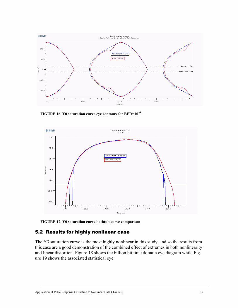
FIGURE 16. Y0 saturation curve eye contours for BER=10-9

FIGURE 17. Y0 saturation curve bathtub curve comparison

5.2 Results for highly nonlinear case

The Y3 saturation curve is the most highly nonlinear in this study, and so the results from this case are a good demonstration of the combined effect of extremes in both nonlinearity and linear distortion. Figure 18 shows the billion bit time domain eye diagram while Fig-ure 19 shows the associated statistical eye.


FIGURE 18. Y3 saturation curve time domain eye for one billion bits

FIGURE 19. Y3 saturation curve statistical eye

Figure 20 is a comparison of eye diagram contours at 10-9, with the time domain contour shown in blue and the statistical analysis contour show in red. Since the duration of the time domain simulation was only a billion bits, it is likely that the time domain contour is slightly optimistic while the statistical analysis contour is slightly pessimistic.

The bathtub curves for the Y3 saturation curve are shown in Figure 21, again with the time domain curve and its confidence limits shown in blue while the statistical analysis curve is shown in red. The statistical analysis result definitely appears to be pessimistic while the time domain result is still probably a little optimistic.


FIGURE 20. Y3 saturation curve eye contours for BER=10-9

FIGURE 21. Y3 saturation curve bathtub curve comparison

The effect of numerical artifacts in Figure 19 is much greater than we usually see, and Fig-ure 22 is much more representative of a typical statistical eye diagram. In Figure 22, the channel discontinuities were reduced by a factor of two and continuous time linear equal-ization (CTLE) was introduced in the receiver. The resulting statistical eye still shows a distinct increase in the outer amplitude at the edges of the eye; however, the inner eye is much better behaved. The increase in outer amplitude at the edge of the eye seems to occur whenever the channel is nonlinear.


Figure 22 also shows the statistical analysis bathtub curve in red and a bathtub curve for a 10 million bit simulation in black. This is also a more typical relationship between statisti-cal analysis and time domain simulation.

FIGURE 22. Y3 saturation curve with reduced channel discontinuities and improved equalization

6.0 Application to PAM4

A nonlinear PAM4 channel offers additional challenges to pseudo-pulse based statistical analysis. Figure 23 shows the eye diagram for a PAM4 signal over a relatively short non-linear channel. Note in particular that the outer eyes have much less height than the inner eye. When we applied pseudo-pulse based statistical analysis directly to this case, the inner eye was too small and the outer eyes were too big.

FIGURE 23. Eye diagram for PAM4 over nonlinear channel


We’ve obtained much better results by modifying the symbol amplitudes in the statistical analysis while using the pseudo-pulse response produced for the NRZ modulation. That is, we introduced an inner amplitude factor such that the symbol amplitudes in the statisti-

cal analysis must be modified by the symbol voltage factors . The

overall process is

1. Run the nonlinear channel with the same PRBS11 NRZ data pattern used in Section 5.0 for NRZ modulation. Extract a pseudo-pulse response from that waveform.

2. Run an additional set of PAM4 symbols to measure the symbol amplitudes. The symbol sequence we used was 00000002222222221111111113333333. Measure the amplitude in the middle of each section of repeating symbols and calculate a symbol voltage fac-tor .

3. Apply PAM4 statistical analysis to the pseudo-pulse response, using the modified sym-bol voltage factors.

Figure 24 is an example of the resulting eye contour comparison to time domain simula-tion results, using NRZ symbols in the pseudo-pulse method and offsetting the symbol voltages as described above. The pseudo-pulse results are optimistic compared to the time domain simulation results; however the contour shapes, sizes and positions for the time domain simulation and pseudo-pulse statistical analysis generally resemble each other.

FIGURE 24. Contour comparison when using NRZ symbols and identified symbol voltages

Statistical analysis eye heights using this method were compared to time domain simula-tion eye heights for simulations of ten million symbols. Channel length was varied from

a

1 1– a–3

---------------- 1 a+3

------------ 1, , ,–

a


10 inches to 35 inches in 5 inch steps, and the same four different degrees of nonlinearity were used as for NRZ in Section 5.0.

FIGURE 25. Nonlinear PAM4 eye height comparison for BER=10-3

FIGURE 26. Nonlinear PAM4 eye height comparison for BER=10-6

While the results are not perfect, they do represent a useful engineering approximation. Consider, furthermore, that the error count for a 10-6 error rate in a ten million symbol simulation is relatively small; so the variance of the time domain results, though not shown, can be expected to be significant at that error rate.


7.0 Summary

This paper has offered an engineering approach to the analysis of nonlinear data channels, in the sense that the methods presented are approximations whose accuracy should be determined before the results are used to make engineering decisions. In that sense, we have presented an evaluation of accuracy under conditions that include a combination of extreme nonlinearity and extreme linear distortion.

We have presented two methods for extracting a pulse response from a time domain wave-form, and have demonstrated that such a pulse response provides useful insights into chan-nel equalization. We have also demonstrated that pulse response based statistical analysis using such a pulse response can produce useful estimates of a channel’s error rate. Finally, we have shown how this statistical analysis method can be modified to produce useful per-formance estimates for nonlinear PAM4 channels.

8.0 References1. Donald Telian, Michael Steinberger, Barry Katz, “New SI Techniques for Large System

Performance Tuning”, DesignCon2016, January 2016.

2. Philip R. Bevington, Data Reduction and Error Analysis for the Physical Sciences, pg. 40, McGraw-Hill, copyright 1969.

3. Prof. Shu Lin, Cathy Liu and Michael Steinberger, “A Brief Tour of FEC for Serial Link Systems, tutorial 10-TU1, DesignCon2015, January 27, 2015.

4. I. J. Good, “On the Inversion of Circulant Matrices”, Biometrika, Vol. 37, No. 1/2, pg. 185-6, June 1950.

5. Steinberger, Wildes, Higgins, Brock and Katz, “When Shorter isn’t Better”, DesignCon2010, February 2, 2010.


Documents

Application of Pulse Response Extraction to Nonlinear Data ... · Application of Pulse Response Extraction to Nonlinear Data Channels 4 The pulse response analysis methods described