Embed Size (px)
Citation preview

DEVELOPMENT OF THE ULTRASHORT PULSE NONLINEAR OPTICAL
MICROSCOPY SPECTRAL IMAGING SYSTEM
A Dissertation
by
ANTHONY CHIEN-DER LEE
Submitted to the Office of Graduate Studies of
Texas A&M University
in partial fulfillment of the requirements for the degree of
DOCTOR OF PHILOSOPHY
August 2011
Major Subject: Biomedical Engineering

Development of the Ultrashort Pulse Nonlinear Optical Microscopy Spectral Imaging
System
Copyright 2011 Anthony Chien-der Lee

DEVELOPMENT OF THE ULTRASHORT PULSE NONLINEAR OPTICAL
MICROSCOPY SPECTRAL IMAGING SYSTEM
A Dissertation
by
ANTHONY CHIEN-DER LEE
Submitted to the Office of Graduate Studies of
Texas A&M University
in partial fulfillment of the requirements for the degree of
DOCTOR OF PHILOSOPHY
Approved by:
Chair of Committee, Alvin T. Yeh
Committee Members, Andreas Holzenburg
Kristen Maitland
Kenith Meissner
Head of Department, Gerard Coté
August 2011
Major Subject: Biomedical Engineering

iii
ABSTRACT
Development of the Ultrashort Pulse Nonlinear Optical Microscopy Spectral Imaging
System. (August 2011)
Anthony Chien-der Lee, B.S., The University of Texas at Austin
Chair of Advisory Committee: Dr. Alvin T. Yeh
Nonlinear Optical Microscopy (NLOM) has been shown to be a valuable tool for
noninvasive imaging of complex biological systems. An effective approach for
multicolor molecular microscopy is simultaneous excitation of multiple fluorophores by
broadband sub-10-fs pulses. This dissertation will discuss the development of two
spectral imaging systems using the principles of nonlinear optical microscopy for pixel-
by-pixel spectral segmentation of multiple fluorescent spectra. The first spectral system
is reliant on a fiber-optic cable to transmit fluorescent signal to a spectrometer, while the
second is based on a spectrometer with an aberration-corrected concave grating that is
directly coupled to the microscope. A photon-counting, 16-channel multianode
photomultiplier tube (PMT) is used for both systems.
Custom software developed in LabVIEW controls multiple counter cards as well as a
field-programmable gate array (FPGA) for 1 Hz acquisition of 256x256x16 spectral
images. Biological specimens consisting of multicolor endothelial cells and zebrafish
will be used for experimental verification. Results indicate successful spectral

iv
segmentation of multiple fluorophores with a decrease in signal-to-noise ratio in the
FPGA-based imaging system.

v
ACKNOWLEDGEMENTS
First and foremost, I would like to thank my committee chair, Dr. Yeh, for his support
throughout my time here in the biomedical engineering department. He has guided me
through a research project which I initially thought to be beyond my abilities.
I would also like to thank Dr. Vitha of the Microscopy and Imaging Center. My results
would not have been possible without his assistance in the development of the optical
hardware for the second spectral system. His technical knowledge in optics has been
invaluable as well.
Last but not least, I would like to thank the rest of my committee, the department faculty,
my friends, and family for being here during my Ph.D. and providing an unforgettable
experience at Texas A&M University.

vi
NOMENCLATURE
CFP Cyan Fluorescent Protein
CW Continuous Wave
DAQ Data Acquisition
DIO Digital Input/Output
DMA Direct Memory Access
EC Endothelial Cell
ECFP Enhanced Cyan Fluorescent Protein
EYFP Enhanced Yellow Fluorescent Proten
FPGA Field-programmable Gate Array
FWHM Full-width at Half Maximum
GFP Green Fluorescent Protein
HDL Hardware Description Language
IPL Inner Plexiform Layer
KLM Kerr Lens Mode-locking
NA Numerical Aperture
NI National Instruments
NLOM Nonlinear Optical Microscopy
NOMS Nonlinear Optical Microscopy System
NOMSIS Nonlinear Optical Microscopy Spectral Imaging System
NOMSISv1 Nonlinear Optical Microscopy Spectral Imaging System Version 1

vii
NOMSISv2 Nonlinear Optical Microscopy Spectral Imaging System Version 2
PMT Photo-multiplier Tube
RTSI Real-time Systems Integration
SHG Second Harmonic Generation
SNR Signal-to-noise Ratio
TPF Two Photon Fluorescence
TTL Transistor-transistor Logic
UI User Interface
VISA Virtual Instrument Software Architecture
YFP Yellow Fluorescent Protein

viii
TABLE OF CONTENTS
Page
ABSTRACT .............................................................................................................. iii
ACKNOWLEDGEMENTS ...................................................................................... v
NOMENCLATURE .................................................................................................. vi
TABLE OF CONTENTS .......................................................................................... viii
LIST OF FIGURES ................................................................................................... x
LIST OF TABLES .................................................................................................... xiii
CHAPTER
I INTRODUCTION ................................................................................ 1
II THEORY OF NONLINEAR OPTICAL MICROSCOPY .................. 6
2.1 Lasers .................................................................................... 6
2.2 Nonlinear Optical Signals ..................................................... 10
III NONLINEAR OPTICAL MICROSCOPY SYSTEM ......................... 15
3.1 NOMS System Setup ............................................................ 15
3.2 Laser Scanning ...................................................................... 18
3.3 Photon Counting .................................................................... 21
3.4 Software Development .......................................................... 22
IV NONLINEAR OPTICAL MICROSCOPY SPECTRAL IMAGING
SYSTEM .............................................................................................. 33
4.1 Fiber-based Spectral Assembly ............................................. 33
4.2 Software Development .......................................................... 36
ix
CHAPTER Page
4.3 Limitations of Spectral Acquisition ...................................... 42
4.4 Directly-coupled Spectral Assembly ..................................... 43
V FIELD-PROGRAMMABLE GATE ARRAYS ................................... 46
5.1 Field-programmable Gate Array Basics ................................ 46
5.2 Software Development .......................................................... 48
VI EXPERIMENTAL VALIDATION ..................................................... 56
6.1 Optical Collection Efficiencies ............................................. 56
6.2 Noise Removal ...................................................................... 62
6.3 In Vitro Imaging of an Angiogenic System .......................... 64
6.4 Spectral Analysis of Multicolor Zebrafish... ......................... 67
VII CONCLUSION AND RECOMMENDATIONS ................................. 72
REFERENCES .......................................................................................................... 74
APPENDIX A ........................................................................................................... 78
APPENDIX B ........................................................................................................... 131
APPENDIX C ........................................................................................................... 139
VITA ......................................................................................................................... 149

x
LIST OF FIGURES
FIGURE Page
2.1 Schematic of a standard laser ..................................................................... 7
2.2 Energy diagram of absorption and emission .............................................. 8
2.3 KLM setup for a pulsed laser ..................................................................... 10
2.4 Quantum well diagram for two photon excitation fluorescence ................ 11
2.5 Calculated T(ω) for a 10-fs (blue) and 100-fs (red) pulse .......................... 13
2.6 Integrated two-photon power spectrum versus pulse duration ................... 14
3.1 NOMS system setup ................................................................................... 16
3.2 NOMS microscope setup ........................................................................... 17
3.3 3D mouse tail tendon .................................................................................. 18
3.4 Laser scanning patterns using (a) raster and (b) triangle waveforms ......... 19
3.5 Mouse tail imaging using (a) raster and (b) triangle scanning patterns ..... 20
3.6 Counter timing example ............................................................................. 22
3.7 NOMS state chart ....................................................................................... 24
3.8 State machine template ............................................................................... 25
3.9 Stage initialization code ............................................................................. 26
3.10 UI event handler example........................................................................... 27
3.11 Open channels state S2 ............................................................................... 28
3.12 Acquire data state S3 .................................................................................. 30
3.13 Analyze data state S4 ................................................................................. 31

xi
FIGURE Page
3.14 Save data state S5 ....................................................................................... 32
4.1 NOMSISv1 system setup ........................................................................... 34
4.2 NOMSISv1 optical setup with (a) schematic of the changes made
within the microscope and (b) spectrometer setup ..................................... 35
4.3 Channel activation ...................................................................................... 37
4.4 Data processing .......................................................................................... 38
4.5 Wavelength selection and graph configuration .......................................... 39
4.6 Nonlinear Optical Microscopy Spectral Imaging System interface ........... 41
4.7 NOMSISv2 spectrometer setup .................................................................. 44
5.1 FPGA trigger detection .............................................................................. 49
5.2 FPGA counting channels ............................................................................ 50
5.3 FPGA data storage ..................................................................................... 52
5.4 Reading from FIFO .................................................................................... 55
6.1 System comparisons ................................................................................... 60
6.2 Noise removal ............................................................................................ 63
6.3 Collected (a) pre-processed and (b) post-processed data ........................... 64
6.4 TPF spectra for CFP, GFP, and YFP ......................................................... 65
6.5 Spectral analysis of endothelial cells ......................................................... 66
6.6 Spectral graph of zebrafish eye .................................................................. 68
6.7 Discrete masking of the zebrafish eye ........................................................ 69
6.8 Spectral subtraction to isolate (a) EYFP and (b) ECFP ............................. 70
6.9 Autofluorescence of wild-type zebrafish ................................................... 70

xii
FIGURE Page
6.10 Multicolor zebrafish eye expressing ECFP and EYFP with a view (a) of
the whole eye and (b) zoomed into the retina ............................................ 71

xiii
LIST OF TABLES
TABLE Page
4.1 Dispersion of Horiba concave grating ........................................................ 45
5.1 Pulse transitions. ......................................................................................... 51
6.1 Experimental configurations with calculated SNR. ................................... 61

1
CHAPTER I
INTRODUCTION
Nonlinear Optical Microscopy (NLOM) systems provide a non-invasive method of
imaging dynamic and complex biological processes over a period of time. Using
femtosecond pulses, nonlinear signals can be collected from endogenous and exogenous
markers by means of two photon excitation and second harmonic generation. Two-
photon excitation spectra can be calculated as
T(ω) |∫ (ω
0
) (ω
) d |
(1.1)
where (ω) represents the pulse electric field in the frequency domain and Ω is the
iterative variable for integration across all frequency components. By overlapping the
two-photon excitation spectra with the molecular two-photon absorption of an excitable
fluorophore γ(ω0), two-photon transition probability can then be represented as a
proportional relationship,
∫ γ(ω0) |∫ (ω0
) (
0
ω0
)d |
dω0
0
(1.2)
where ħω0 is the transition energy. Two-photon transition probability represents the
likelihood of nonlinear signal generation. Therefore, maximizing this value is highly
desirable to enhance NLOM signals.
____________
This dissertation follows the style of Optics Express.

2
The calculation shows that optimizing two-photon transition involves broadening of the
spectral profile for the pulses, which occurs as the pulse is shortened in the time domain.
The condition can be met with pulses in the fs range, typically 100 fs for standard
NLOM systems. As pulse duration further decreases towards a magnitude of 10,
spectral bandwidth increases respectively because of the Fourier relationship. This
broadening allows for simultaneous excitation of multiple fluorophores, a characteristic
which does not exist in 100 fs pulses [1,2]. When applied to an NLOM laser pulsed at
sub-10 fs, the spectral bandwidth is broadened to ~125 nm, allowing for a time-efficient
spectral imaging modality with no detrimental effect to image quality [1]. By using
detectors and optical filters, fluorescent and second harmonic signal can be transferred
and separated in imaging software to display individual components of a biological
sample[3]. Ultimately, NLOM imaging provides a fast and efficient way to generate two
and three dimensional images quickly and noninvasively.
The usage of ultrashort pulses also benefits from an improvement in depth-based NLOM
imaging. Three-dimensional NLOM imaging depth is typically limited by the
generation of out-of-focus fluorescence at the surface of the sample as laser power
intensity is increased [4,5]. When the sample’s fluorescent signal degrades as the laser
focuses into the sample due to scattering, the fluorescence intensity at the focus
approaches that of the fluorescence intensity generated at the surface. This limitation
exists for transform-limited 100 fs pulses used with most NLOM lasers. By introducing
dispersion and generating a sub-10 fs chirped pulse with an ultrashort-pulse laser, the
3
highly concentrated fluorescent signal at the focus is expected to significantly reduce
depth limitation of NLOM imaging due to the dispersive characteristics of ultra-short
pulses [6].
Present-day NLOM systems typically use individual photomultiplier tubes set at specific
wavelengths to detect fluorescent signal. In order to collect signal at different
wavelengths, either the optical filter needs to be adjusted manually or an additional
detector needs to be used in conjunction. Additionally, these systems use a laser with
~100 fs pulse width which have a much narrower excitation spectrum [1]. Tuning the
laser to a new central wavelength is an additional requirement for spectral imaging [7].
The continuous tuning and calibration required for these systems makes spectral
experimentation on living specimen a difficult and time-consuming task. Although
useful for systems containing one or two fluorescent specimen, the information provides
little insight to the emission spectra of samples containing multiple fluorophores. In
order to understand the true chemical and biological composition of specimens, the
system should detect signal with respect to emission wavelength using an ultrashort
pulse laser. The ability to distinguish between spectral characteristics of specimens with
closely related emission spectra is also highly desired.
The solution is to design a multi-channel detection system using a detector capable of
acquiring signal across a large spectrum, an ultrashort pulse laser allowing for broadband
excitation, and National Instruments (NI) hardware to perform high-speed data

4
acquisition. The primary goal of the dissertation is the design of a high-speed 16-
channel NLOM system using a sub-10 fs laser.
In order to begin development of the 16-channel imaging system, a two-channel imaging
system must be designed capable of acquiring images matching that of the lab’s current
imaging software. Images acquired with this software could then be used as a reference
for verification of the new imaging system. Known as the Nonlinear Optical
Microscopy System (NOMS), the system is a fully functional 2-channel imaging system
capable of acquiring a 3-dimensional stack of images automatically. The data may be
saved in binary format for ease of analysis using third-party programs such as
MATLAB. Additionally, NOMS can open saved files to review images that have been
previously acquired. After completion, the system can be expanded for 16-channel
multispectral NLOM imaging, resulting in the Nonlinear Optical Microscopy Spectral
Imaging System (NOMSIS).
LabVIEW is the chosen form of programming for NOMSIS development because of its
ability to communicate between the hardware and software with ease. Unlike standard
text-based programming languages such as C and Java, LabVIEW uses a graphical
programming language known as “G” which follows a dataflow programming
architecture. Graphical programming is much like writing out an algorithm on paper.
By laying out functional “blocks” which perform a specific task and connecting them
with “wires ” the software can directly convert the layout to machine code for execution.

5
This leads to a quick and easy solution to tasks which would normally take many lines of
typed code. Additionally, graphical programming allows for multiple starting points
where data execution begins. Computers equipped with multi-core processors can
automatically take advantage of this implementation and load-balance the instructions
between multiple threads. Because text-based programming languages execute using the
top-to-bottom approach, writing a program to take advantage of multi-core processors is
much more difficult. LabVIEW usage has grown significantly in the years as it proves
capable of creating complex programs to solve modern engineering problems [8-10].
After development, verification and comparison of the systems are performed.
Experimental datasets verify spectral delineation of multiple fluorophores, as well as
provide an insight to the optical collection efficiencies of the designs.

6
CHAPTER II
THEORY OF NONLINEAR OPTICAL MICROSCOPY
Background and theory behind the principles of operation of the system is discussed in
Chapter II. Principles of laser operation are reviewed in Section 2.1, and theory behind
nonlinear optical signals is discussed in Section 2.2.
2.1 LASERS
Due to the necessity of using lasers in NLOM, understanding their basic principles is
essential. The term laser was initially derived as an acronym from Light Amplification
from Stimulated Emission of Radiation. Stimulated emission, or highly organized
emission of light, is the key concept in the term which leads to the generation of laser
light.
A typical laser is generated from a highly reflective cavity containing two mirrors, one
fully reflective while the other is semi-reflective. A gain medium, the Ti:Al2O3 crystal,
within the cavity is excited via a pump source. The pump can vary from sources such as
an external light, a secondary laser, or an electrical current. For our lab, the pump
source is another laser, an Nd:YVO4. As seen in Figure 2.1, the pump source excites the
molecules from the gain medium into a higher energy level through absorption.

7
Figure 2.1. Schematic of a standard laser.
When the molecules return to ground state, spontaneous emission of a photon of lesser
energy is generated as illustrated in Figure 2.2. This photon is at 800 nm for our system.
Spontaneous emission lacks a uniform direction; however a few of the photons will be
emitted at a direction parallel to the cavity. This means the photon will bounce back
from the mirror and return to the gain medium, allowing for what is known as stimulated
emission. Stimulated emission takes place when an emitted photon collides with an
electron already in an excited state. The electron will fall to ground state and generate
an additional photon. Without the mirrors within the cavity, stimulated emission would
cause a quick depletion of excited molecules.

8
Figure 2.2. Energy diagram of absorption and emission.
Population inversion, a state when more molecules are in the excited state than ground
state, exists when the mirrors in the cavity reflect the photons to propagate a continuous
cycle of stimulated emission. Finally, lasing occurs as the amplified light within the
cavity exits through the semi-reflective mirror.
After establishing a continuous wave (CW) laser, we need to understand the mechanism
known as mode-locking which generates a pulsed laser. The bandwidth of a laser pulse
in the time domain is the Fourier transform of the spectral width in the frequency
domain. Because of the inverse relationship between the time and frequency domains, a
pulse with the broadest possible spectrum, or the greatest possible number of cavity
modes, will also have the shortest possible time duration. The phases for each of the
lasing cavity modes are locked. Constructive interference between the superposition of
cavity modes creates a high-intensity pulse, whereas destructive interference cancels out
the energy, allowing for a series of pulses.
9
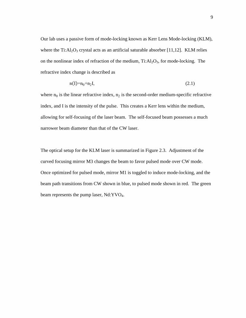
Our lab uses a passive form of mode-locking known as Kerr Lens Mode-locking (KLM),
where the Ti:Al2O3 crystal acts as an artificial saturable absorber [11,12]. KLM relies
on the nonlinear index of refraction of the medium, Ti:Al2O3, for mode-locking. The
refractive index change is described as
n( ) n0 n (2.1)
where n0 is the linear refractive index, n is the second-order medium-specific refractive
index, and is the intensity of the pulse. This creates a Kerr lens within the medium,
allowing for self-focusing of the laser beam. The self-focused beam possesses a much
narrower beam diameter than that of the CW laser.
The optical setup for the KLM laser is summarized in Figure 2.3. Adjustment of the
curved focusing mirror M3 changes the beam to favor pulsed mode over CW mode.
Once optimized for pulsed mode, mirror M1 is toggled to induce mode-locking, and the
beam path transitions from CW shown in blue, to pulsed mode shown in red. The green
beam represents the pump laser, Nd:YVO4.

10
Figure 2.3. KLM setup for a pulsed laser.
2.2 NONLINEAR OPTICAL SIGNALS
The polarization of high-intensity pulses interacting with electric fields can be
represented as
i i k(1) i k
( ) k i k
( ) k l (2.2)
which is the Taylor series expansion for the nth
order susceptibility of the sample, (n)
.
Linear microscopy, such as one-photon confocal fluorescence, can be described by the
(1)
term. The remaining higher order describes nonlinear effects. NLOM traditionally

11
relies on two principle theories: second harmonic generation arising from the (2)
term,
and two-photon fluorescence (TPF) arising from the (3)
term.
Two-photon excitation microscopy relies on the simultaneous absorption of two photons
and generation of fluorescent emission through molecular relaxation. As illustrated in
Figure 2.4, a molecule absorbs two photons of low energy which satisfies the transition
requirements to go from ground state E1 to excited state E2. The resulting output from
intramolecular vibrational relaxation is an emission photon with energy greater than a
single absorbed photon. For our system, the absorption will arise from the 800 nm
ultrashort pulses.
Figure 2.4. Quantum well diagram for two photon excitation fluorescence.
Second harmonic generation (SHG), also known as frequency doubling, arises from the
unique nature of a specimen. Nonlinear interaction between the laser and a sample of
non-centrosymmetric structure allow for effective combination of two incident photons,

12
generating a new photon of twice the energy and frequency, and at half the wavelength.
Specimens which possess centrosymmetric structure have no SHG signal because of the
non-zero second harmonic coefficient. SHG microscopy is prevalent in many biological
studies, such as the cornea of the eye and collagen protein, both of which naturally
possess the unique qualities required for SHG.
While TPF signal only originates from the molecular relaxation shortly after absorption,
SHG signal is only generated when the pulse is actively hitting the sample. Because
both TPF and SHG signals are derived from the same theory for nonlinear optics, no
additional modification is needed in a nonlinear optical imaging system as long as the
detection wavelengths are within range.
Nonlinear signal generation can be calculated as a relation to pulse duration, Tp. Using
Equation 1.1, two-photon power spectrum T(ω) is calculated using a duration-dependent
Gaussian approximation for a transform-limited pulses as shown in Figure 2.5. Using 10
and 100 fs pulses for comparison, we observe a much broader waveform for the two-
photon transition energy in the 10 fs pulse. The data indicates that the usage of a shorter
pulse significantly increases two-photon excitation due to the increased bandwidth.

13
Figure 2.5. Calculated T(ω) for a 10-fs (blue) and 100-fs (red) pulse.
The conclusion can be further validated by plotting two-photon power spectrum for
multiple pulse durations. Shown in Figure 2.6, we observe a slope of -1 which indicates
that two-photon transition probability will increase proportionally with 1/Tp. At this
point Equation 1.2 is limited by the pulse, thus shortening of pulse duration is ideal for
maximizing nonlinear signals. However there are limitations as transition probability is
not constricted to just the pulse, but also the molecular two-photon absorption.
Assuming a transform-limited infinitely short pulse, two-photon excitation becomes
infinitely broad in the time domain. Because the molecular absorption profile is still
Gaussian, the fluorophore is unable to absorb all frequency components of the laser.
250 300 350 400 450 500 5500
0.1
0.2
0.3
0.4
0.5
0.6
0.7
0.8
0.9
1
Two-photon Transition Energy (hc/E)
Inte
nsity (
A.U
.)

14
This causes the transition probability of Equation 1.2 to yield diminishing returns as
pulse duration becomes shorter [6].
Figure 2.6. Integrated two-photon power spectrum versus pulse duration.
10-14
10-13
108
109
1010
1011
Pulse Duration (s)
Inte
gra
ted T
wo-p
hoto
n P
ow
er
Spectr
um
(A
.U.)

15
CHAPTER III
NONLINEAR OPTICAL MICROSCOPY SYSTEM
With the proper knowledge of NLOM principles, we can now develop an imaging
system known as the Nonlinear Optical Microscopy System (NOMS). NOMS system
development is discussed in Section 3.1. Section 3.2 describes the technique to control
scanning mirrors. Section 3.3 discusses the photon counting procedure, and software
development is examined in Section 3.4.
3.1 NOMS SYSTEM SETUP
NOMS hardware setup is illustrated in Figure 3.1. The laser first passes through
dispersion compensation optics. Dispersion compensation mirrors are necessary to
create negative dispersion in order to cancel out the positive dispersion induced by the
microscope optics. This pre-compensation ensures a high peak power at the focus and
prevents a loss in excitation and detection efficiencies. A neutral density filter (not
shown in figure) can be placed anywhere along the laser pathway to attenuate power.
The laser then passes through computer-controlled dual-axis galvanometers, which are
further discussed in Section 3.2. Upon entering the microscope, the laser passes through
a telescope which guides the laser to be imaged onto the back focal aperture of the
objective lens as shown in Figure 3.2. The laser passes through the microscope, and
signal from the sample returns through a dichroic short pass mirror. The mirror is

16
Figure 3.1. NOMS system setup.
chosen to be a 635 nm short-pass in order to minimize back-scattering of the laser into
the detection optics, as desired signal NLOM signal for the system is not greater than
635 nm. The signal passes through a tube lens and two long-pass dichroic mirrors.
These mirrors separate incoming signal into two channels, one channel for optical signal
shorter than 430 nm, and one pathway for signal shorter than 620 nm but greater than
430 nm. Each channel enters selective band-pass mirrors which isolate desired
wavelength pass-bands. Finally, focusing lenses are used for entrance into the
photomultiplier tubes (PMT). The PMTs convert the optical signals into electrical
signals and transfers the data into discriminators which further translate the electrical
signal into transistor-transistor-logic (TTL) pulses. These pulses are counted and
detected by the computer, as described in Section 3.3, finally rendering a working image.
A stage-control signal sent by the computer allows for automated imaging in the z-
dimension. The usb-controlled signal instructs the stage to change position with a
precision up to 1/20th
of a µm. By changing the focus of the sample and collecting a

17
series of images, a 3-dimensional image can be generated from a stack of 2-dimensional
data.
Figure 3.2. NOMS microscope setup.
Experimental validation is performed by acquiring SHG signal from a mouse tail tendon.
Mouse tail tendons are an excellent sample to use for testing purposes in NLOM due to
the ease of generating second harmonic signal. The tendon is placed under the objective
and SHG signal is collected by NOMS. Using sawtooth scanning and voltage-guided
mirrors, NOMS collects and saves a stack of 2-d images. Post-processing of the stack
creates a working figure for the tendon as illustrated in Figure 3.3. The data concludes
that NOMS is a capable method for non-invasive image generation of biological
samples.

18
Figure 3.3. 3D mouse tail tendon.
3.2 LASER SCANNING
Laser-guided scanning is a standard for modern optical imaging systems. In order to
ensure the laser passes across all desired portions of a sample, various scanning patterns
are used. For 2-dimensional X-Y galvanometer scanning, the most common forms are
raster and triangle scanning. Raster scanning, shown in Figure 3.4(a), is a series of line
scans originating from the same side and moving across the sample’s X-axis. In Figure
3.4(b), triangle scanning moves the laser in reverse direction on every other line.

19
Figure 3.4. Laser scanning patterns using (a) raster and (b) triangle waveforms.
The scanning mirror galvanometers, are sensitive to electrical voltage, within a range
typically ±15V. As the voltage changes, the mirrors move to corresponding positions
with high accuracy and precision. This allows for voltage-based control to generate the
desired scanning waveforms. Because guidance of the laser is limited to two mirrors,
these scanning patterns need to be simulated as one continuous flow. The x-axis
scanning is created using voltage generation of a sawtooth waveform for raster scanning,
and a triangle waveform for triangle scanning. The y-axis scanning pattern is always a
sawtooth waveform.
Although both patterns should theoretically generate the same images, minute
differences still exist when data is acquired. Raster scanning of the tendon generates
signal distortion at the left and right sides of the image as seen in the Figure 3.5(a). This
is due to the sudden transition of the mirror’s x-axis to return to the original location
while signal collection and image processing continuously occurs. The issue can be
reduced by increasing the scanning time which allows the mirror to move at a slower
pace. As seen with the usage of triangle scanning in Figure 3.5(b), this distortion issue is

20
virtually eliminated. Because triangle scanning has the x-axis continue from the end of
each line rather than returning to the original location, mechanically-induced distortion
of the image is not an issue. However upon closer examination of the triangle-scanned
tendon, there exists a slight discontinuity in the fibers which can be described as “ agged
edges.” The issue comes from the small variations in the scanning pattern arising from
the reverse-scanning of the sample on every return segment of the triangle waveform
pattern. This discontinuity prevents images from being as clear as the datasets acquired
from raster-scanning. Ultimately, a slow, raster-based scanning pattern would be the
ideal form of laser-scanning for system development.
Figure 3.5. Mouse tail imaging using (a) raster and (b) triangle scanning patterns.

21
3.3 PHOTON COUNTING
In photon counting, signal from the sample is picked up by a PMT which creates a spike
in its output signal. This output signal is in the form of an electrical current which is
read by a preamplifier/discriminator (F-100T, Advanced Research Instruments Corp.).
The discriminator generates a TTL pulse whenever the electrical current from the
detector exceeds a manually specified threshold setting. The TTL pulses are counted
directly and correspond to the intensity of a pixel on a grayscale intensity graph. Proper
signal triggering and timing algorithms must be understood in order for photon counting
to properly generate images. Figure 3.6 is an example of photon counting which is
properly triggered and interpreted. By generating an internal clock signal corresponding
to the desired scanning speed, it can act as both a starting trigger signal as well as a pixel
divider. Although not shown on the figure, the X-Y scanning mirrors are also triggered
with this signal. As photons are picked up and pulsed through the discriminator, the
hardware will then count the pulses and store them within memory for image processing.
The integer counts arrive into the computer as a series of arrays. NOMS rearranges the
arrays as they arrive to create a final 256x256 image.

22
Figure 3.6. Counter timing example.
3.4 SOFTWARE DEVELOPMENT
NOMS takes advantage of two standardized LabVIEW programming algorithms: the
Standard State Machine, and the User Interface (UI) Event Handler. The Standard State
Machine operates on a process of dividing a program into various subsections, each of
which runs a particular segment of code. The computer traverses between each
subsection, known as a state, based on particular conditional events within the code or
actions taken by the computer operator. Ultimately, the State Machine will loop back to
the beginning to start once more, or end up at a STOP state which instructs the program
to terminate. The UI Event Handler is the second LabVIEW programming algorithm
used for NOMSIS. This algorithm is used when a program requires user input among
numerous controls on the front panel, each of which performs a unique task. When a

23
task is completed, the program control returns to wait for the next UI command. If
illustrated as a state machine, the UI Event Handler would be a single state which
continuously returns to itself upon completion. By integrating both the Standard State
Machine and the User Interface Event Handler algorithms, complex programs can be
efficiently created within the LabVIEW software.
NOMS programming summary is divided into seven states as seen in Figure 3.7.
nitialization state S0 opens communication with the LUDL lectronics’ MAC5000
stage controller for the microscope. In order for 3-dimensional data acquisition to work
properly, NOMS must get a successful pingback from the stage controller indicating
successful data initialization. This allows NOMS to send commands directly to the stage
which controls vertical movement along the Z-axis. If the response has failed, the user
can choose to check the connections and retry the initialization. The second option
would be to continue with stack acquisition disabled, in which case NOMSIS will
disable 3-dimensional imaging processes. This initialization state only needs to be run
once during the operation of the software, which is why the state diagram does not return
to the S0 state upon completion.

24
Figure 3.7. NOMS state chart.
Complete code for NOMS is too extensive for placement within text, so it may be
referenced within Appendix A. Only the essential portions of NOMS for each state will
be discussed within the chapters. LabVIEW implementation of the state machine
architecture is simplified by usage of a template built into the software. By nesting a
case structure within a while loop, a shift register may be used to determine transition
states. Figure 3.8 shows the most basic layout of the State Machine template, with the
Initialize state, corresponding to S0, set to execute first. When developing NOMS, the
stage initialization driver provided by LUDL Electronics is placed inside the case
S0
S1
S2
S3 S4
S5
S6
S0: Initialization
S1: Wait for User Input S2: Open Channels
S3: Acquire Data
S4: Analyze Data
S5: Save Data
S6: Emergency Exit
Data Flow
User Input Error Detection

25
structure. LabVIEW then updates the next transition state and loops back to begin the
next state.
Figure 3.8. State machine template.
Implementation of state S0 requires the usage of drivers provided from LUDL
Electronics. These drivers allow for the integration and detection of the microscope
stage into the NOMS software. Figure 3.9 shows the code, which is used as a sub-vi,
and placed inside the Initialize state of NOMS. By making use of NI Virtual Instrument
Software Architecture (VISA), artificial drivers can be programmed for third-party
hardware and become recognizable by LabVIEW.

26
Figure 3.9. Stage initialization code.
The code uses the hardware address generated by NI VISA for USB-based initialization
of the mechanical stage of the microscope. If the software executes without error,
NOMS will transition to state S1. Failure to execute properly will allow the user to
check for errors and retry, or simply continue without stage-controlled imaging.
User Interface state S1 is the primary state where user-controlled operations are
controlled. This state checks which controls on the interface are being interacted with by
the user. The majority of interactions will result in a small change to the front panel,
such as “graying” out different locations followed by the state returning to itself.
Implementation is performed by using an Event Structure. The event structure is used to
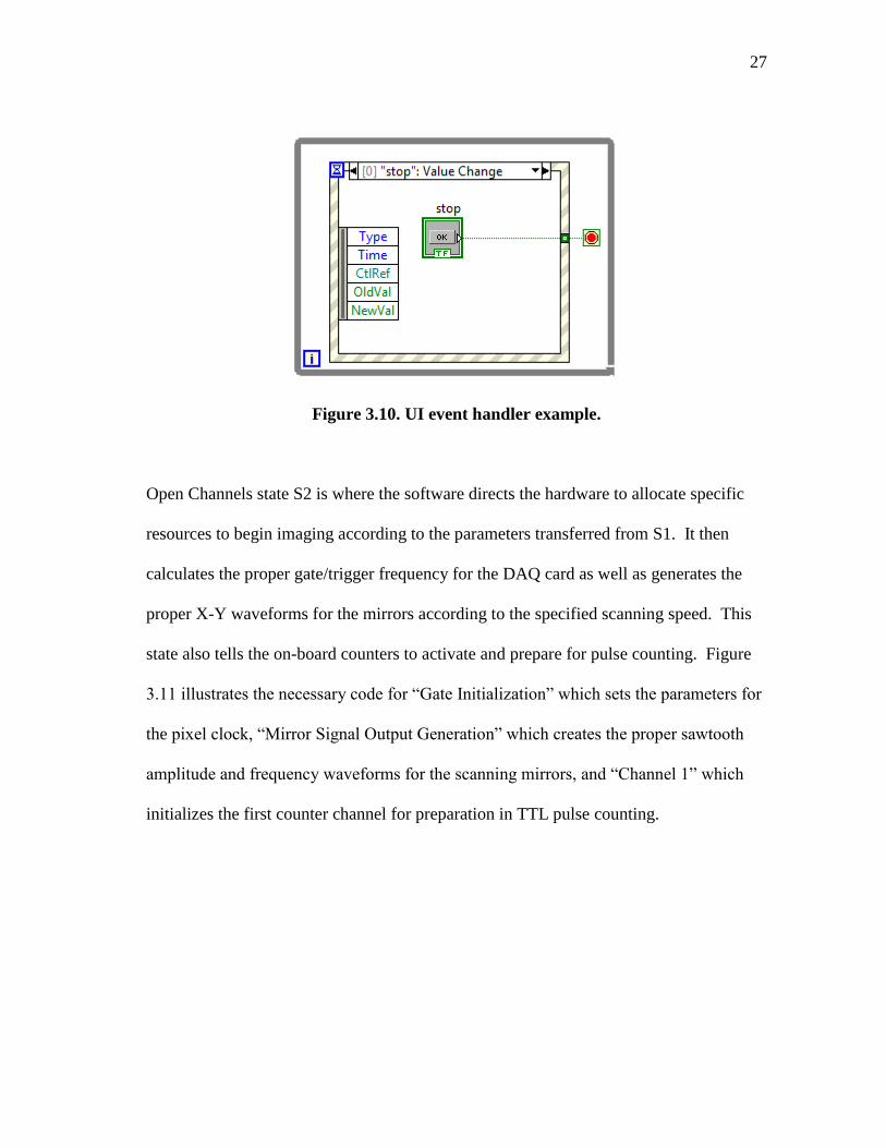
execute code when certain user-based events are executed. Figure 3.10 shows a simple
UI Event Handler example if the “stop” button is pressed on-screen. The corresponding
action is to stop the while loop. For NOMS, once the state detects the “Start” button
being pressed, the computer proceeds to state S2.
27
Figure 3.10. UI event handler example.
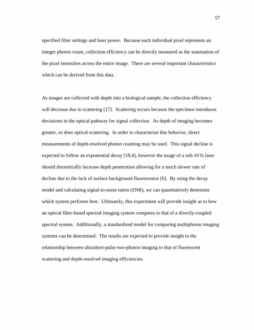
Open Channels state S2 is where the software directs the hardware to allocate specific
resources to begin imaging according to the parameters transferred from S1. It then
calculates the proper gate/trigger frequency for the DAQ card as well as generates the
proper X-Y waveforms for the mirrors according to the specified scanning speed. This
state also tells the on-board counters to activate and prepare for pulse counting. Figure
.11 illustrates the necessary code for “Gate nitialization” which sets the parameters for
the pixel clock “Mirror Signal Output Generation” which creates the proper sawtooth
amplitude and frequency waveforms for the scanning mirrors and “Channel 1” which
initializes the first counter channel for preparation in TTL pulse counting.

28
Figure 3.11. Open channels state S2.

29
Acquire Data state S3 is where actual imaging takes place. Data is received from the
activated counter channels of S2 and split into segments of 4,096 pixels at a time as seen
in Figure 3.12. Because the counter cards only count upward from pixel-to-pixel,
subtraction must take place to determine the true count corresponding to each pixel. The
short C script in the formula node performs this subtraction when the array is received
from the counter. This data is then reshaped from a 1-dimensional array into an 8x256
pixel 2-dimensional array and displayed to the screen. The process is repeated 31
additional times to generate the entire 256x256 pixel image. When continuously
scanning an image, the code takes the prior 8x256 array and replaces it with the updated
array, allowing for smooth updating of the image. The counters are then deactivated,
and the laser is then instructed to diverge from the sampling region.

30
Figure 3.12. Acquire data state S3.
Analyze Data state S4 is primarily for multiple-scanning calculations. Because many
experiments desire the ability to rescan the area to improve signal-to-noise ratio within
an image, a state must exist to determine whether additional scans are necessary to
complete the acquisition of the current image layer. This check is performed in the
sequence structure of Figure 3.13. An internal Scan Counter is used to determine
whether the current scan number matches that of the user-specified value. If the value
has not yet been reached, the software is instructed to return to state S2 to perform an

31
additional scan. The corresponding pixels in the new image are then directly added to
the respective portion in the old one, creating a new image.
Figure 3.13. Analyze data state S4.
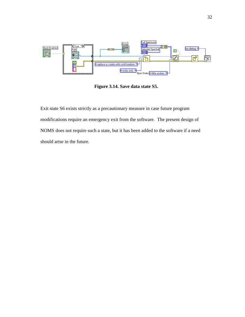
Save state S5 is used to transfer the data within the intensity images into readable files in
the computer hard drive. The code, shown in Figure 3.14, concatenates the two images
generated in NOMS as a 256x256x2 3-dimensional array, and saves the data as a binary
file in little-endian format. The little-endian format stores data corresponding to the
least-significant byte first. This characteristic is important as many computation
applications such as MATLAB can only read data stored in little-endian format. Data
stored in big-endian, with the most-significant byte first, will be loaded with corrupted
data. State S5 also detects whether or not 3-dimensional stack acquisition has completed
acquisition. If incomplete, a command is sent to the MAC5000 stage to move the stage
along the Z-axis at the specified step size, and the system returns to state S2 to take the
next image.
32
Figure 3.14. Save data state S5.
Exit state S6 exists strictly as a precautionary measure in case future program
modifications require an emergency exit from the software. The present design of
NOMS does not require such a state, but it has been added to the software if a need
should arise in the future.

33
CHAPTER IV
NONLINEAR OPTICAL MICROSCOPY SPECTRAL IMAGING SYSTEM
Spectral acquisition of samples is important when given biological systems with multiple
intrinsic and extrinsic fluorophores. This spectral data can be used for delineation and
separation of colors, ultimately acting as a non-invasive method for separation of
different biological components. The system has been named the Nonlinear Optical
Microscopy Spectral Imaging System (NOMSIS). This chapter discusses the
development of two variations of NOMSIS, to be referred as NOMSISv1 and
NOMSISv2. The reasons for the development of two versions will be examined as well.
4.1 FIBER-BASED SPECTRAL ASSEMBLY
Hardware development of NOMSISv1 is summarized in Figure 4.1. The optical setup is
identical to that of NOMS up until detection. Instead of using the optical band-pass
filters, fluorescent signal from the sample is directed through a tube lens coupled to an
optical fiber and into a spectrometer housing containing a 16-channel PMT [13] as
illustrated in Figure 4.2(a). The PMT then converts the optical fluorescence into sixteen
channels of analog current. The electrical current is translated by an array of
discriminators into 16-channel TTL pulses for photon counting.

34
Figure 4.1. NOMSISv1 system setup.
Like NOMS, TTL pulses are detected by the NI PCI-6602 counter card, but two cards
are used instead of one to accommodate all 16 channels. The software then uses the
values of the counters and rearranges them as intensity pixels. Finally, LabVIEW
renders a working image directly onto the front panel.
The multimode optical fiber with high numerical aperture (NA = 0.22) with a large core
(910 µm) delivers fluorescent signal to the remotely located spectrometer optics. Within
the spectrometer, NOMSISv1 incorporates a Czerny-Turner setup in a Littrow
configuration for Figure 4.2(b). Exiting the fiber, the first optical component is an
achromatic lens (d = 38.1 mm, f = 90.0 mm) for collimating divergent light. The light is
then sent to a diffraction grating (53-067-455R, Richardson Grating) blazed at 530 nm.
A focusing lens of f = 75.0 mm is then used to demagnify the diffracted light onto the
16-channel detector (R5900U-00-L17, Hamamatsu).

35
Figure 4.2. NOMSISv1 optical setup with (a) schematic of the changes made within
the microscope and (b) spectrometer setup.
Linear dispersion of the diffraction grating represents the spectral extent per unit width.
This dictates the spectral range that the spectrometer can detect. The formula for linear
dispersion is represented as
d
dx cos( )
mdLB
1 .5 nm (4.1)
where is the diffraction angle m is the diffraction order, d is the groove density of the
grating, and LB is the focal length of the focusing lens. Setting the central wavelength to
490 nm, we yield a spectral range of 350-630 nm, with each channel covering
approximately 17.58nm of the spectrum.

36
4.2 SOFTWARE DEVELOPMENT
Modification of the user interface, as well as key components within NOMS source code
is essential in making a working system for NOMSIS. The first portion of NOMS code
requiring changes is the channel activation of the counters from S2 of the state diagram.
Activation of each individual counting channel was expanded from simply 2 channels, to
16. Figure 4.3 illustrates the activation of channels 6-8. We can see that each channel
possesses the same code for activation, with exception to the I/O input task which
corresponds to the respective data line. The remaining channels not on the figure are
activated in a similar fashion. One additional requirement is the modification of the
counting mechanism from DMA to Interrupt, as seen in the invoke node.
State S3 requires modification as well. Figure 4.4 illustrates the processing of incoming
pulses. The data is collected and subtracted from the previous element because of the
upward counting of the individual counters. This separates the individual elements of
the array as actual pulse counts. Once again, the code is duplicated and source code for
all 16 channels can be implied from the figure.

37
Figure 4.3. Channel activation.

38
Figure 4.4. Data processing.

39
Significantly differing from NOMS, the code in Figure 4.5 is used for the front panel
selection boxes, allowing for the on-off display of user-desired spectral channels. The
series of Boolean selections are formatted into an array and processed by the for loop.
The loop will sum together all of the individual 256x256 images that have been selected
by the user on the front panel, creating a representative intensity image. The loop also
generates the x-axis to be used for the spectral wavelengths of each channel.
Figure 4.5. Wavelength selection and graph configuration.
As seen in Figure 4.6, the NOMSIS software displays this array according to selected
controls on the front panel. While actively collecting data, the imaging parameters are
replaced by a spectral influence graph. This graph shows an on-the-fly spectral

40
representation of the sample as a whole by taking the summation of all the pixels in each
corresponding channel. Each summation is representative of a single point on the
spectrum and can be directly plotted onto the graph. The sample used in the image was
endothelial cells expressing green fluorescent protein (GFP) embedded within a collagen
matrix.
Selection 1 of Figure 4.6 shows the entire sample by selection of the channels
corresponding to the peaks in the spectrum. We can clearly see both SHG signal from
collagen and TPF of GFP from the cells. Selection 2 isolates the collagen by simply
choosing the SHG channels, and selection 3 isolates the GFP signal from the cells. This
effectively allows for quick spectral segmentation of biological specimen for uniquely
different fluorescent markers.

41
Figure 4.6. Nonlinear Optical Microscopy Spectral Imaging System interface.

42
4.3 LIMITATIONS OF SPECTRAL ACQUISITION
Upon completion of the initial 16-channel system, one significant limitation became
apparent. The imaging speed must be greatly reduced in order to prevent an internal
buffer error. Because the two NI PCI-6602 counter cards contain only three Direct
Memory Access (DMA) channels per card, high-speed imaging is limited to a maximum
of six channels at a time. DMA is a method used to transfer data into memory without
involving the computer’s C U. Without enough DMA channels, counting mechanism is
changed to Interrupt – a processing mechanism which requires the usage of the CPU for
data transfer. Unfortunately in order to use all sixteen channels at once and prevent the
buffer from overflowing, the imaging speed needs to be greatly reduced – the fastest
possible speed being sixteen seconds per image. Because previous studies have shown
that cellular migration can occur at a rate well over 1 µm/min [14], sixteen seconds per
image becomes insufficient for experiments collecting large quantities of data.
The alternative to this problem is to use a field-programmable gate array (FPGA) from
National Instruments (PCI-7811R). Since an FPGA has much more memory, sixteen
physical channels of data can be taken in a single high-speed DMA channel. This
implementation should theoretically solve the issue with the counter cards and allow
scanning frequency up to 1 image per second [15], and has motivated the need to create
a new spectral system, NOMSISv2.

43
4.4 DIRECTLY-COUPLED SPECTRAL ASSEMBLY
The system layout for NOMSISv2 is quite similar to NOMSISv1, with hardware
changes made starting from the spectrometer. In addition to using FPGA, which will be
discussed in detail in the following chapter, a more simplified approach to designing a
spectrometer is desired as well.
Instead of using an optical fiber, NOMSISv2 directly couples the fluorescence detection
optics to the microscope as seen in Figure 4.7. At the side port of the microscope, an
achromat of f = 35.0 mm will be used to demagnify the image of the exit aperture of the
objective lens. An adjustable slit is used to control signal from the demagnifying lens.
In order to mimic the optical fiber of NOMSISv1, the slit is open to the same distance as
the diameter of the optical fiber. A mirror then directs this light onto an aberration-
corrected concave holographic grating (533-01-370, Horiba) which can be directly
transferred to the 16-channel detector (R5900U-200-L16, Hamamatsu). The use of a
concave grating has been shown to simplify the optical setup for spectral imaging due to
its unique shape, allowing for the input slit to be directly imaged onto a PMT [16].

44
Figure 4.7. NOMSISv2 spectrometer setup.
The linear dispersion of the Horiba concave grating is
d n
dx 10
cos( ) cos γ
knL
(4.2)
where is the diffraction angle, is the tilt angle of the detector plane relative to the
normal of the diffracted beam, k is the diffraction order, n is the groove density, and LH
is the effective focal length. Unlike the grating used in NOMSISv1, the concave grating
has nonlinear dispersion, becoming shorter as the wavelength increases. Dispersions
from the formula are summarized in Table 4.1 for the central wavelength of each
channel of the detector.
Mirror
Achromat Lens
Concave Aberration-corrected Blazed Grating (Horiba)
Microscope Objective
Microscope Field Lens
Mirror
16-channel PMT

45
Table 4.1. Dispersion of Horiba concave grating.
Channel
Number
Dispersion
(nm/mm)
Central
Wavelength (nm)
0 21.4 350.7
1 21.1 371.8
2 20.7 392.5
3 20.4 412.9
4 20.0 432.9
5 19.7 452.7
6 19.4 472.0
7 19.0 491.0
8 18.7 509.7
9 18.3 528.0
10 18.0 546.0
11 17.7 563.7
12 17.3 580.9
13 16.9 597.9
14 16.6 614.4
15 16.3 630.7
The results show the corresponding dispersion, with the shorter wavelengths possessing
a larger channel width. Varying slightly from NOMSISv1, the spectral range for
NOMSISv2 is from 340-639 nm.

46
CHAPTER V
FIELD-PROGRAMMABLE GATE ARRAYS
A field-programmable gate array (FPGA) is used for many engineering applications to
streamline signal processing and data analysis. To overcome the limitations of
NOMSISv1, an FPGA is used to collect high-speed data. Section 5.1 provides a brief
overview of FPGA technology, and Section 5.2 details the integration of FPGA code
into NOMSISv2.
5.1 FIELD-PROGRAMMABLE GATE ARRAY BASICS
An FPGA is a programmable integrated circuit capable of running an instruction set,
known as hardware description language (HDL), at speeds independent of the
computer’s clock speed. This allows a complex program to run on the oldest of
computers while avoiding hardware speed issues. FPGAs can also interface with
external systems, allowing for a smooth integration of FPGA into existing technology.
As modern-day technology advances, more and more systems are incorporating the
usage of FPGA hardware.
Inside the board, an FPGA consists of digital hardware known as logic blocks which are
interconnected with one another. Once the HDL code is compiled and synthesized, the
programmable interconnects turn on or off respectively, and a unique digital circuit is

47
then created to represent the desired system. The configuration is saved as a single
bitfile which can be stored directly to a computer’s hard drive. Analogous to a
computer’s executable file a bitfile represents the set of DL instructions that have been
programmed by the user for the FPGA. This allows the FPGA to immediately configure
the digital circuit without re-synthesis of HDL code.
HDL is a low-level programming language which directly interfaces with digital logic
circuits and memory registers. To make FPGA programming as familiar as possible to
the standard LabVIEW developer, NI created the FPGA Module which masks the
complexity of writing HDL code. Users may program the FPGA with a specialized
LabVIEW function set designed specifically for FPGA boards.
The NI PCI-7811R FPGA was chosen for photon counting implementation. The FPGA
has an internal clock of 40 MHz. If each clock cycle is used to check on the High/Low
status of an incoming pulse, it would take two clock cycles to determine a pulse has
passed. This means photon counting can only be as fast as half the internal clock, 20
MHz. By default, the discriminators have a pulse width of 10 ns. Because the FPGA can
only check the digital lines once every 25 ns, a 10 ns pulse may be completely missed by
the FPGA. Therefore, the discriminators will need to have their pulses expanded to a
value greater than or equal to 25 ns. With NOMSISv2, an adjustment of 30 ns pulse
width will be used to be safe.
48
The 16-channel data is stored inside the FPGA's high-speed FIFO (first in, first out)
memory stack. In the case of a 1-second scan, the FPGA would be configured to store
data once every 15.26 µs. From there, NOMSISv2 can pull the data at its own pace for
image rendering. The FPGA software will have basic input/output elements. By using it
as sub-element within the NOMSIS software, the FPGA code can be directly integrated
into present LabVIEW code.
5.2 SOFTWARE DEVELOPMENT
FPGA code will replace the channel-activation sub-vi within state S2 for NOMSIS. To
begin LabVIEW FPGA-based photon counting, the FPGA requires some form of
starting signal to act as the trigger. For this, we can use the same pixel clock as
generated for NOMSISv1 by interconnecting the signal into an FPGA input channel.
Using the FPGA palette, the corresponding data channel can be placed within a while
loop to continuously poll the input until the signal has arrived.
FPGA trigger detection code is shown in Figure 5.1. Because the pixel clock acts as a
trigger mechanism for photon counting, the signal must pass directly to the FPGA for
activation of the counting channels. The signal enters the FPGA board via the Real-time
System Integration (RTSI) cable internally attached to the data acquisition board within
the computer. RTSI buses act as the interconnection for different hardware systems, in
this case the FPGA board and the data acquisition board. The while loop will

49
continuously check the status of the RTSI channel until it receives a digital high value,
thus exiting the loop and entering the counting portion of code.
Figure 5.1. FPGA trigger detection.
FPGA counting consists of two portions: pulse counting, and data storage. Figure 5.2
demonstrates the code required for the pulse counting to take place. The green logic line
entering from the left is from the trigger detection output. Once the trigger gives the
active signal to begin counting, the internal 40 MHz clock of the FPGA is activated for a
single-cycle timed while loop, meaning it executes the code within the loop on every
rising edge of the clock.

50
Figure 5.2. FPGA counting channels.
The code first checks if Clear Counts control is 1 or 0. Initially it will always begin as 0,
then checks the signal lines of each respective digital input/output (DIO) channel. If the
DIO channel transitions from 0 to 1, then the counter will increment itself. Any other
combination will leave the counter unchanged, as care must be taken to not increment
the counter until the entire pulse has been detected and passed through the channel.
Table 5.1 demonstrates this behavior of the counters as the FPGA takes measurements
from each DIO. Action will only be taken when pulse transitions are detected. Once
Clear Counts changes to a 1, every counting channel will reset itself to zero counts.
This acts as a reset mechanism to restart the counting at the beginning of each pixel.

51
Table 5.1. Pulse transitions.
Status Old Value New Value Transition Detected
No Pulses 0 0 No
Pulse Received 0 1 Yes
Pulse Still Active 1 1 No
Pulse Exit 1 0 No
Data storage for the FPGA is seen in Figure 5.3. FPGAs have a built-in stack for
temporary memory storage. This stack is known as a first-in, first-out (FIFO) stack. In
memory systems, FIFO stacks are beneficial when receiving large blocks of data on a
continuous basis. This data can be removed and processed from the stack by the
computer starting from the element that came first, as the name FIFO implies. If data
arrives faster than the computer can process, FIFO stacks are typically implemented. In
the case of high-speed photon counting, FIFO is essential. The FIFO buffer will store
incoming photon counts and remove them when the computer has caught up to the
remaining data elements to be processed.

52
Figure 5.3. FPGA data storage.
53
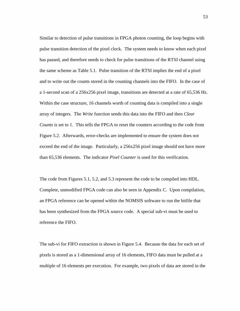
Similar to detection of pulse transitions in FPGA photon counting, the loop begins with
pulse transition detection of the pixel clock. The system needs to know when each pixel
has passed, and therefore needs to check for pulse transitions of the RTSI channel using
the same scheme as Table 5.1. Pulse transition of the RTSI implies the end of a pixel
and to write out the counts stored in the counting channels into the FIFO. In the case of
a 1-second scan of a 256x256 pixel image, transitions are detected at a rate of 65,536 Hz.
Within the case structure, 16 channels worth of counting data is compiled into a single
array of integers. The Write function sends this data into the FIFO and then Clear
Counts is set to 1. This tells the FPGA to reset the counters according to the code from
Figure 5.2. Afterwards, error-checks are implemented to ensure the system does not
exceed the end of the image. Particularly, a 256x256 pixel image should not have more
than 65,536 elements. The indicator Pixel Counter is used for this verification.
The code from Figures 5.1, 5.2, and 5.3 represent the code to be compiled into HDL.
Complete, unmodified FPGA code can also be seen in Appendix C. Upon compilation,
an FPGA reference can be opened within the NOMSIS software to run the bitfile that
has been synthesized from the FPGA source code. A special sub-vi must be used to
reference the FIFO.
The sub-vi for FIFO extraction is shown in Figure 5.4. Because the data for each set of
pixels is stored as a 1-dimensional array of 16 elements, FIFO data must be pulled at a
multiple of 16 elements per execution. For example, two pixels of data are stored in the

54
FIFO as a series of integer elements from [E0, E1, E2, ..., E31]. E0-E15 represents the
first pixel, while E16-E31 represents the second. To reduce strain on the CPU, 1024
pixels are acquired at once, meaning Number of Elements is set to 16,384. The invoke
node pulls all of the elements from FIFO using Counts.Read, and immediately
reprocesses the data from a 1-dimensional 1x16384 element array into a 3-dimensional
1 x4x 5 array using LabV W’s built-in array functions. The loop afterwards
prepares this array for insertion directly into the front panel of NOMSIS as a processed
image. This process is repeated 64 more times until the entire 256x256x16 image has
been fully acquired. The code is placed as a sub-vi within S3 of the state machine
algorithm.

55
Figure 5.4. Reading from FIFO.

56
CHAPTER VI
EXPERIMENTAL VALIDATION
With two NLOM spectrometers, we need to compare the two setups and determine
which design produces the ideal signal collection, as well as provide datasets as
validation of working systems. Section 6.1 discusses the theoretical and experimental
comparisons between NOMSISv1 and NOMSISv2. Section 6.2 explains data processing
method for noise removal. Sections 6.3 and 6.4 describe experiments for using
NOMSIS as a valid method of spectral imaging and analysis.
6.1 OPTICAL COLLECTION EFFICIENCIES
Optical collection efficiency refers to the ability of the collection optics to detect signal
from incoming fluorescent photons. This limitation is primarily based on the least-
efficient optical component in the detection pathway. Fluorescent signal collection for
the NOMS system is strictly limited by the numerical aperture of the objective. Signal
collection for NOMSISv1 is limited to the numerical aperture of the fiber, whereas
signal collection for NOMSISv2 is limited to the numerical aperture of the optical
grating.
By recording depth-resolved three-dimensional data, a comparison can be made by
observing both of the spectral systems’ image stacks with respect to NOMS data at its
57
specified filter settings and laser power. Because each individual pixel represents an
integer photon count, collection efficiency can be directly measured as the summation of
the pixel intensities across the entire image. There are several important characteristics
which can be derived from this data.
As images are collected with depth into a biological sample, the collection efficiency
will decrease due to scattering [17]. Scattering occurs because the specimen introduces
deviations in the optical pathway for signal collection. As depth of imaging becomes
greater, so does optical scattering. In order to characterize this behavior, direct
measurements of depth-resolved photon counting may be used. This signal decline is
expected to follow an exponential decay [18,4], however the usage of a sub-10 fs laser
should theoretically increase depth penetration allowing for a much slower rate of
decline due to the lack of surface background fluorescence [6]. By using the decay
model and calculating signal-to-noise ratios (SNR), we can quantitatively determine
which system performs best. Ultimately, this experiment will provide insight as to how
an optical fiber-based spectral imaging system compares to that of a directly-coupled
spectral system. Additionally, a standardized model for comparing multiphoton imaging
systems can be determined. The results are expected to provide insight to the
relationship between ultrashort-pulse two-photon imaging to that of fluorescent
scattering and depth-resolved imaging efficiencies.

58
The optical collection efficiency can be quantitatively represented as the spectrometer’s
etendue, which characterizes the ability of a system’s acceptance of light. Geometric
etendue, represented as G, is a function of the area S representing the source of light and
the numerical aperture NA expressed as
( ) (6.1)
In an ideal system with perfect transmission of light, two optical systems can be directly
compared by taking their ratio of etendue, or
( )
( ) ( )
( )
(6.2)
Because the optical setup for NOMSISv1 and NOMSISv2 use the same geometric area,
the etendue ratio can be further simplified to
( )
( ) ( )
( )
(6.3)
which implies the etendue of NOMSISv2, G2, is 29% more efficient than G1, the etendue
of NOMSISv1. The calculation is based on the assumption of 100% transmission of
light through all optical components, which is not the true representation of the optical
setup. By factoring in the transmission efficiencies of optical components such as the
gratings and mirrors, a more accurate representation is
( )
( )
( )
( )
(6.4)
where T1 represents the average transmission efficiency of the concave grating, T2 is the
average transmission efficiency of the linear grating, and T3 through T5 represent the

59
transmission through the coated lenses. Ultimately, the optical setup of NOMSISv2
should theoretically be 48% more efficient than that of NOMSISv1.
Unfortunately this calculation also assumes ideal photon collection of the electrical
components with equivalent SNR. As mentioned in Chapter IV, several counting
electronics were modified in order to fit the parameters required for FPGA counting in
NOMSISv2. Direct comparison through theoretical equations is limited because of the
manual thresholding required of the discriminators. The only way to fully compare the
two systems is experimentally through analysis of the data stacks and raw photon counts.
The experiment is performed on the upright microscope using a green fluorescent slide
and imaged in software to collect the raw photon counts. The fluorescent slide is imaged
completely through top to bottom, and the photon counts are plotted with respect to
depth. Laser power and sample location is fixed to prevent any deviations in data due to
variables. SNR comparisons will ultimately determine the ideal imaging system.
The experiment is performed using four different NLOM setups. NOMS is to be used as
a control for a point of reference. NOMSISv1 is then used to take the exact same stack.
An intermediary setup, using the fiber-based optics of NOMSISv1 with the FPGA
counting of NOMSISv2 helps differentiate between the root cause of any significant
SNR differences between the optics and electronics. Finally, the experiment is repeated
one last time using the NOMSISv2 setup. Two goals are desired in the experiment. The
first is proper exponential decay of the signal with respect to depth, verifying the

60
different NLOM setups as properly collected data. The second is to determine the SNR
of the systems using the data, effectively providing the true conclusion as to which
optical system performs better in its current state.
Figure 6.1 summarizes the results in the graph of raw photon counts versus depth in µm.
2-channel data is displayed using the entire dataset from NOMS. The spectral systems
are displayed using the summation of data in the five strongest channels, effectively
representing the photons collected for spectral full-width at half-max (FWHM).
Choosing only the channels representing FWHM minimizes the effects of noise on both
spectral systems and allows for irrelevant noise to be excluded from the true SNR. As
expected, an exponential decay is observed for all system setups.
Figure 6.1. System comparisons.

61
The absolute maxima for all setups should exist at the same depth. For the fiber-based
spectral detector, a lack of water under the immersion objective created a delay in signal
generation. We can take note that the actual peak for the setup is roughly 5% higher
than presented in the figure which should slightly increase the SNR. Because the
fluorescent slide is not infinitely thick, the expected value for noise in SNR would be
that of the raw photon counts after the laser has passed through the slide. Therefore,
calculation of the SNR can be performed by taking the ratio between the strongest point
in the signal curve with respect to the corresponding signal at the drop-off point when
the laser has passed through the sample. The results are summarized in Table 6.1.
Table 6.1. Experimental configurations with calculated SNR.
NLOM Setup Optics Electronics SNR
NOMS Filters Counter Cards 61.1
NOMSISv1 Fiber-based Spectrometer Counter Cards 20.5
Intermediary Fiber-based Spectrometer FPGA 7.78
NOMSISv2 Directly-coupled Spectrometer FPGA 6.20
NOMSISv1 is expected to have a fair reduction in SNR compared to NOMS due to the
reduction in NA and attenuation of optical transmission from the spectrometer. As the
experimental setup changed from NOMSISv1 to the Intermediary, a surprising reduction
of nearly 3x SNR is observed. Based on the green line of Figure 6.1, the results show
that the usage of the new discriminators with FPGA-based photon counting caused a

62
significant reduction in the maximum signal. The root cause may be from a loss in
efficiency in counting by using an FPGA as well as an increase in noise from the new
discriminator array. The data indicates that NOMSISv1 is the ideal system when taking
spectral images of samples that are not time-limited.
6.2 NOISE REMOVAL
High quality images are a necessity for processing and presentation of experimental
datasets in NLOM. Because the discriminators for NOMS and NOMSIS are highly
sensitive to electromagnetic interference from the environment, a few datasets may
easily be clouded by noise. This is evident by the random speckle pattern apparent
within images. For our NLOM systems, noise can be removed by a simple algorithm of
equating the noisy pixel to a non-problematic neighbor. The image resolution is high
enough to perform the task without causing aberrations in the data.
LabVIEW code for noise removal is shown in Figure 6.2. The corresponding intensity
data enters the loop from the left, with a user-specified noise threshold set into the
threshold control. Because LabVIEW supports basic C programming code, the data can
be passed into a formula node which contains the algorithm for noise removal. The code
analyzes data row-by-row, and compares the intensity difference from one pixel to the
next. If this difference exceeds the threshold value, the noisy pixel is set equal to the
intensity of its neighbor. The current state of NOMS and NOMSIS do not implement

63
this feature automatically, however future work could implement the threshold control
into the front panel of the software for automated noise removal.
Figure 6.2. Noise removal.
Figure 6.3 validates this process as seen in the pre-processed and post-processed images
for despeckling of a zebrafish eye. The unprocessed dataset on the left has a fair number
of pixels plagued with noise. This is most easily identified by the bright spots in the
dark portions of the image. With a threshold level of 70 for this particular sample, a
total of 1,150 noise pixels covering roughly 1.8% of the image are removed via post-
processing. This process saves valuable time and prevents the need for reacquisition of
datasets when noise exists throughout an image.

64
Figure 6.3. Collected (a) pre-processed and (b) post-processed data.
6.3 IN VITRO IMAGING OF AN ANGIOGENIC SYSTEM
Experimental validation of NOMSISv1 is performed using an in vitro model that mimics
angiogenesis [13]. Human endothelial cells (EC) expressing green (GFP), yellow
(YFP), and cyan fluorescent proteins (CFP) are mixed and stimulated to penetrate a 3D
well consisting of collagen matrix. Given time to incubate, the cells assemble into
multicellular structures surrounding an open lumen. The goal of the experiment is to
delineate multiple colored ECs from a body consisting of multiple fluorescent
fluorophores.

65
For initial reference spectra, confluent populations of each fluorescent EC cell line are
imaged within a 12-well plate. Data for corresponding spectra are normalized and
shown in Figure 6.4.
Figure 6.4. TPF spectra for CFP, GFP, and YFP.
The mixed sample of ECs within the collagen is allowed to incubate and invade the
collagen for 60 hours before imaging. Figure 6.5 illustrates a resulting representative
image of the system taken near the monolayer of the sample. The numbered spectra
correspond to the regions marked in the NOMSIS image, with false color applied to
illustrate the locality of fluorescence. SHG from the collagen is left in grayscale.

66
Figure 6.5. Spectral analysis of endothelial cells. Scale bar 15 µm.
Region 1 corresponds to expression of second harmonic signal from collagen. Regions 2
through 4 correspond to endothelial cells expressing GFP, YFP, and CFP, respectively.
Region 5 corresponds to the lumen of the cell, which lacks signal as expected and
corresponds to dark count of background signal. The data shows that the system can
clearly identify individual spectra expressed from multiple fluorophores with just a
single scan of data.

67
6.4 SPECTRAL ANALYSIS OF MULTICOLOR ZEBRAFISH
The zebrafish eye has become an important model for study due to the similarities in
morphology to the human eye [19-21]. The fast life cycle of the fish, transparency of
the embryo, and the large number of eggs allows for detailed studies to be performed for
analysis of eye development. NOMSISv2 will be validated by a study of zebrafish
expressing multiple fluorescent fluorophores within the eye. Multicolor zebrafish were
provided by researchers from Georgia Health Sciences University and prepared as
described [22]. Mating between the fish have produced an embryo with positive
expression of enhanced CFP (ECFP) from transgene pax6-DF4:gap43-CFP and
enhanced YFP (EYFP) from transgene UAS:gap43-YFP.
EYFP expression is targeted to the retinal bipolar interneurons of the eye, and ECFP
expression is a membrane-tagged reporter and expressed in membranous regions of the
fish. The inner plexiform layer (IPL) is where several retinal neuron subtypes –
including bipolars – make synaptic connections. It can be clearly identified by its unique
semicircular structure within the retina and surrounding the lens. Because the ECFP is
membrane-tagged, the IPL and other synaptic neuropils are labeled strongly since they
are membrane-rich regions. Using the same zebrafish data illustrated in Figure 6.3, the
spectrum is shown in Figure 6.6. The graph clearly indicates two unique fluorophores
represented by the two maxima in the graph at 405 nm and 500 nm. Unlike the dataset
from the ECs, spectral analysis of the zebrafish eye will be performed using subtraction

68
instead of localized analysis. Because the spectral graph represents the image as a
whole, individual pixels can be uniquely classified by applying a mask. When analyzing
pixels corresponding to EYFP, the spectrum will exhibit a strong unique peak
corresponding to the 500 nm channel. Similarly, the pixels corresponding to the
membranous expression of ECFP will have a unique peak at 405 nm. This characteristic
allows us to apply a discrete mask to the data, segmenting the image into ECFP, EYFP,
and background.
Figure 6.6. Spectral graph of zebrafish eye.
The mask in Figure 6.7 represents the discretized image of the zebrafish eye. Each pixel
is processed and assigned a color. Black if there is no signal, blue if the signal is most
likely ECFP, and green if the signal is most likely EYFP. This information can be used
to identify the corresponding fluorescent signal of the fluorophore as well as determine
color assignment when processing an image.

69
Figure 6.7. Discrete masking of the zebrafish eye.
Isolating the individual reporters within the image can be done using simple subtraction
between channels. By taking the individual image corresponding to the yellow and cyan
channels, subtraction from one another yields the regions of the desired fluorophore. As
seen in Figure 6.8(a), subtraction from the yellow channel removes the IPL from the
retina in the eye. The remaining signal from the bipolar neurons remains strong and
visible. Figure 6.8(b) performs the same subtraction, only this time removing yellow
from cyan. The resultant image isolates the IPL as the membranous-tagged reporter.

70
Figure 6.8. Spectral subtraction to isolate (a) EYFP and (b) ECFP.
Endogenous autofluorescence must be accounted for as well. To identify and exclude
the signal caused by autofluorescence, we use a wild type zebrafish with no exogenous
reporters as seen in Figure 6.9. We can clearly identify the areas where untagged bipolar
neurons would exist. The IPL, although visible, is much weaker in signal intensity.
Figure 6.9. Autofluorescence of wild-type zebrafish.

71
After identifying the desired fluorescent markers, we can recombine the initial dataset
and color the morphologically relevant portions of the image as shown in Figure 6.10(a).
The image shows expression of ECFP and EYFP reporters within the eye, with false-
colors blue representing ECFP and yellow representing EYFP. Using the wild-type
zebrafish to identify autofluorescence, the corresponding signal is left in grayscale. The
white box marks a region of distinguishable bipolar interneurons, with the overexposure
in the right part of the eye caused by the angle of the fish during imaging. The dominant
cyan band marked by the arrow within the retina represents the IPL. Figure 6.10(b)
decreases the field of view and displays a close-up of the retina, allowing for a better
look at the neurons. These results show that NOMSISv2 is a valid spectral system for
NLOM, obtaining useful results in biological systems regardless of the reduction
observed in the SNR.
Figure 6.10. Multicolor zebrafish eye expressing ECFP and EYFP with a view (a) of
the whole eye and (b) zoomed into the retina.

72
CHAPTER VII
CONCLUSION AND RECOMMENDATIONS
This study encompassed the development and benefits of using NLOM as a valid form
of spectral imaging. Using the LabVIEW Professional Development System, we
developed an in-house NLOM system for two-channel imaging in multiple dimensions
known as NOMS. Using optical filters, the system is capable of targeting reporters of
known emission wavelengths and generates respective intensity images. NOMS was
validated by a three-dimensional acquisition of a mouse tail tendon. The system is still
used regularly by the Tissue Microscopy Lab for two-channel data acquisition.
Because an ultrashort pulse laser allows for simultaneous excitation of multiple
fluorophores across a large spectrum, acquisition of more than two nonlinear signals
required a new method of collection which motivated development of NOMSISv1.
Using a multimode fiber-optic cable, delivery of fluorescent signal occurred in a
spectrometer isolated from the microscope. A multi-channel PMT detected optical
signals which were diffracted through a grating and allowed for spectral imaging of a
biological system on-the-fly. An angiogenesis model demonstrated the system’s
capabilities of spectral delineation.
Limited DMA channels prevented the system from collecting images at speeds faster
than 16 seconds. The desire for high-speed imaging motivated the development of

73
NOMSISv2. Overcoming this limitation required the use of an FPGA, which also came
with an updated discriminator array. Updating the system motivated a change in the
optics as well. A spectrometer directly coupled to the microscope was chosen in hopes
to increase optical collection efficiency and optimize SNR. Experimental comparison
between the two systems contradicted the calculations, as SNR in NOMSISv2 declined
due to the counting mechanism from either the FPGA or discriminator arrays. Despite
the decline in efficiency, NOMSISv2 performed well in the experimental validation of a
multicolor zebrafish sample. Excitation of EYFP and ECFP yielded spectral data for
bipolar interneurons and the membrane-rich IPL, respectively.
As technology develops, new methods for improving optical efficiency of the system can
be utilized. Future work should involve increasing the collection efficiency of the
spectral systems by identifying new optics with higher NA. Additionally, locating the
source of the significant reduction in SNR is vital to further enhancement of the system.
Whether the reduction was induced by the decrease in photon counting speed required
by the FPGA or poor performance of the new discriminators, identifying the problem
should significantly improve system performance. Since FPGA-based photon counting
was limited to 20 MHz, newer technological advances should increase this limit and
ultimately gain the capability to perform photon counting at ultra-high speeds. By using
newer PMTs capable of 32 channels, spectral resolution may be further enhanced.

74
REFERENCES
1. A. T. Yeh, H. Gibbs, J. J. Hu, and A. M. Larson, "Advances in nonlinear optical
microscopy for visualizing dynamic tissue properties in culture," Tissue
Engineering Part B Rev. 14(1), 119-31 (2008).
2. R. K. Benninger, M. Hao, and D. W. Piston, "Multi-photon excitation imaging of
dynamic processes in living cells and tissues," Reviews of Physiology,
Biochemistry, and Pharmacology 160, 71-92 (2008).
3. P. P. Provenzano, C. T. Rueden, S. M. Trier, L. Yan, S. M. Ponik, D. R. Inman,
. J. Keely and K. W. liceiri “Nonlinear optical imaging and spectral-lifetime
computational analysis of endogenous and exogenous fluorophores in breast
cancer ” Journal of Biomedical Optics 13, 031220 (2008).
4. A. Leray and J. Mertz, "Rejection of two-photon fluorescence background in
thick tissue by differential aberration imaging," Optics Express 14, 10565-10573
(2006).
5. P. Theer and W. Denk, "On the fundamental imaging-depth limit in two-photon
microscopy," Journal of the Optical Society of America A 23, 3139-3149 (2006).
6. S. Pang, A. T. Yeh, C. Wang, and K. E. Meissner, "Beyond the 1/Tp limit: two-
photon-excited fluorescence using pulses as short as sub-10-fs," Journal of
Biomedical Optics 14, 054041 (2009).

75
7. A. J. Radosevich, M. B. Bouchard, S. A. Burgess, B. R. Chen, and E. M. C.
Hillman, "Hyperspectral in vivo two-photon microscopy of intrinsic contrast,"
Optics Letters 33, 2164-2166 (2008).
8. G. Faraco and L. Gabriele “Using LabV W for applying mathematical models
in representing phenomena ” Computers & ducation 49(3), 856-872 (2007).
9. M. A. Alia, T. M. Younes and S. A. Alsabbah “A design of a D self-tuning
controller using LabV W ” Journal of Software ngineering and Applications
4(3), 161-171 (2011).
10. M. A. Alia, T. M. Younes, and M. A. Zalata “Development of equivalent virtual
instruments to PLC functions and networks ” Journal of Software ngineering
and Applications 4(3), 172-180 (2011).
11. J. errmann “Theory of Kerr-lens mode locking: role of self-focusing and
radially varying gain ” Journal of the Optical Society of America B 11, 498-512
(1994).
12. T. Brabec C. Spielmann . F. Curley and F. Krausz “Kerr lens mode locking ”
Optics Letters 17(18), 1292-1294 (1992).
13. A. M. Larson, A. Lee, P.-F. Lee, K. J. Bayless and A. T. Yeh, "Ultrashort pulse,
multispectral nonlinear optical microscopy," Journal of Innovative Optical
Health Sciences 2(1), 27-35 (2009).
14. J. Huth, M. Buchholz, J. M. Kraus, M. Schmucker, G. Wichert, et al.,
“Significantly improved precision of cell migration analysis in time-lapse video

76
microscopy through use of a fully automated tracking system ” BMC Cell
Biology 11(24), 1-12 (2010).
15. C. Buehler, K. H. Kim, U. Greuter, N. Schlumpf, and P. T. C. So, "Single-
photon counting multicolor multiphoton fluorescence microscope," Journal of
Fluorescence 15, 41-51 (2005).
16. L. Yan, C. T. Rueden, J. G. White, and K. W. Eliceiri, "Applications of
combined spectral lifetime microscopy for biology," Biotechniques 41(3), 249-
253 (2006).
17. F. elmchen and W. Denk “Deep tissue two-photon microscopy ” Nature
Methods 2, 932-940 (2005).
18. A. K. Dunn, V. P. Wallace, M. Coleno, M. W. Berns, and B. J. Tromberg,
"Influence of optical properties on two-photon fluorescence imaging in turbid
samples," Applied Optics 39, 1194-1201 (2000).
19. C. B. Kimmel, W. W. Ballard, S. R. Kimmel, B. Ullmann, and T. F. Schilling,
“Stages of embryonic development of the zebrafish ” Developmental Dynamics
203, 253-310 (1995).
20. T. Greiling and J. . Clark “ arly lens development in the zebrafish: a three-
dimensional time-lapse analysis ” Developmental Dynamics 238, 2254-2265
(2009).
21. Z. Li, N. M. Joseph and S. S. aster “The morphogenesis of the zebrafish eye
including a fate map of the optic vesicle ” Developmental Dynamics 218, 175-
188 (2000).

77
22. J. Ariga, S. L. Walker and J. S. Mumm “Multicolor time-lapse imaging of
transgenic zebrafish: visualizing retinal stem cells activated by targeted neuronal
cell ablation ” Journal of Visualized Experiments 43, (2010):
http://www.jove.com/details.php?id=2093.

78
APPENDIX A
NOMS SOURCE CODE
nomsis.vi
Primary vi file for NOMS. Although front panel names it as NOMSIS and there are
controls for spectral control, the features are disabled and the software functions as a 2-
channel NLOM system.
Connector Pane

79
Front Panel

80
Block Diagram
State S0 – Initialization. Sub-vi checks for proper initialization from the microscope
stage. If failure, user is prompted to retry or ignore. Corresponding results will be
shown in the on-screen indicator.

81

82
State S1 – Wait for User Input. Event structure waits for action from the user. If Laser
Divergence is checked, DC voltage signals are sent to the mirrors to minimize laser-
sample interaction. Controls and indicators are set to default value.

83

84
If the Start button is pressed, NOMS sets initial front panel display settings and sets the
next state to S2. If other buttons are pressed, NOMS simply adjusts the visual front
panel accordingly and returns to state S1.
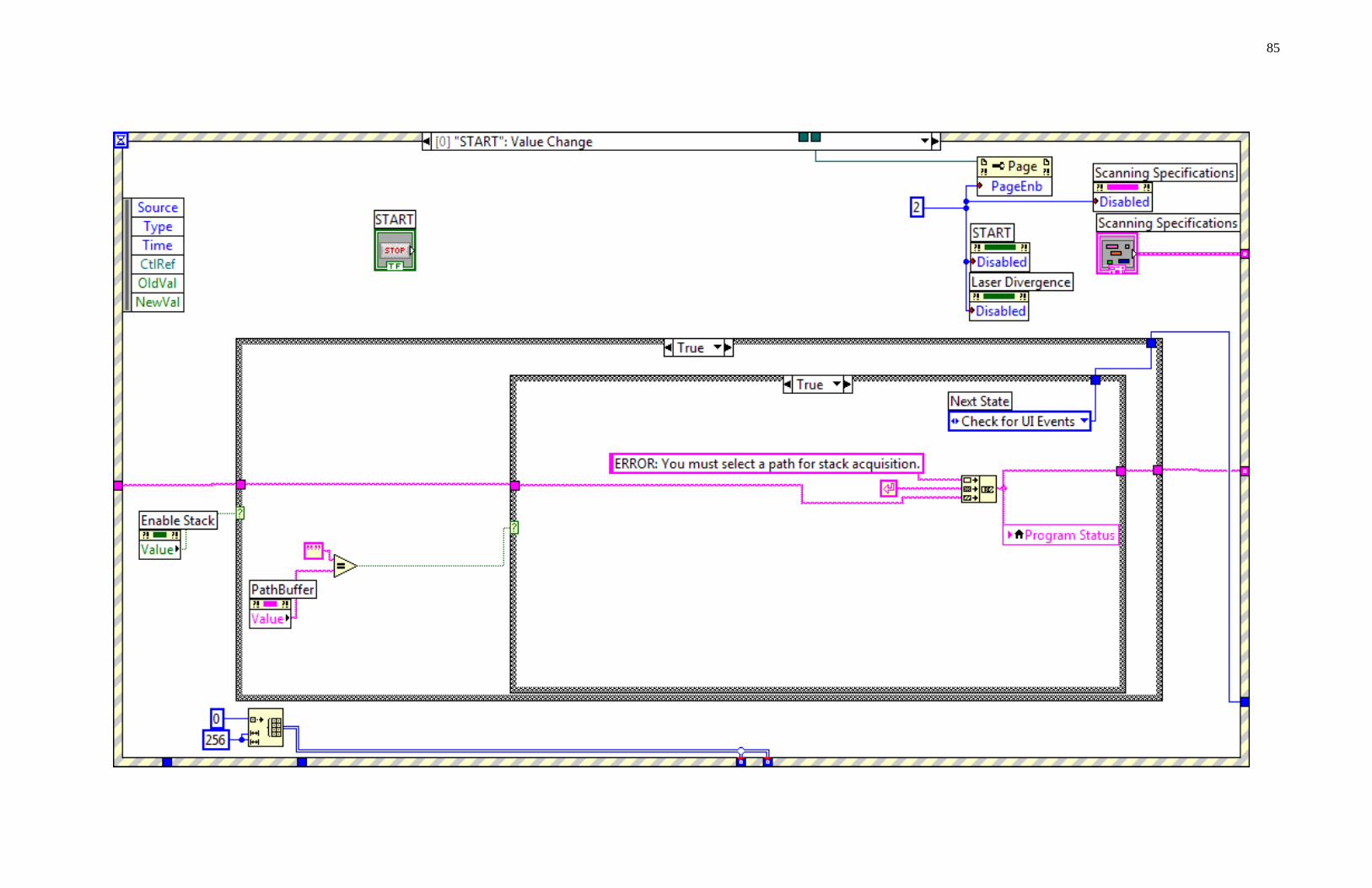
85

86
The current location of the stage is stored into the on-screen indicator. This value is also
used to determine the appropriate offsets when performing 3-dimensional imaging.

87
No action is taken if the Stop button is pressed during S1.

88
If the save button is pressed, next state is set to S5.

89
Aesthetic modifications.

90
Aesthetic modifications.

91
Aesthetic modifications.

92

93
Sub-vi called when Path button is pressed. User is prompted to select a folder, and the path is stored in PathBuffer.

94
Aesthetic modifications.

95
State S2 – Open Channels. Pixel clock frequency is calculated based on user-inputted
speed settings. A counter channel from the DAQ card initializes the waveform. Two
analog output channels are initialized as well, set for amplitude and frequency based on
user-specified settings. Two counter channels are activated on the counter cards for TTL
pulse counting.

96
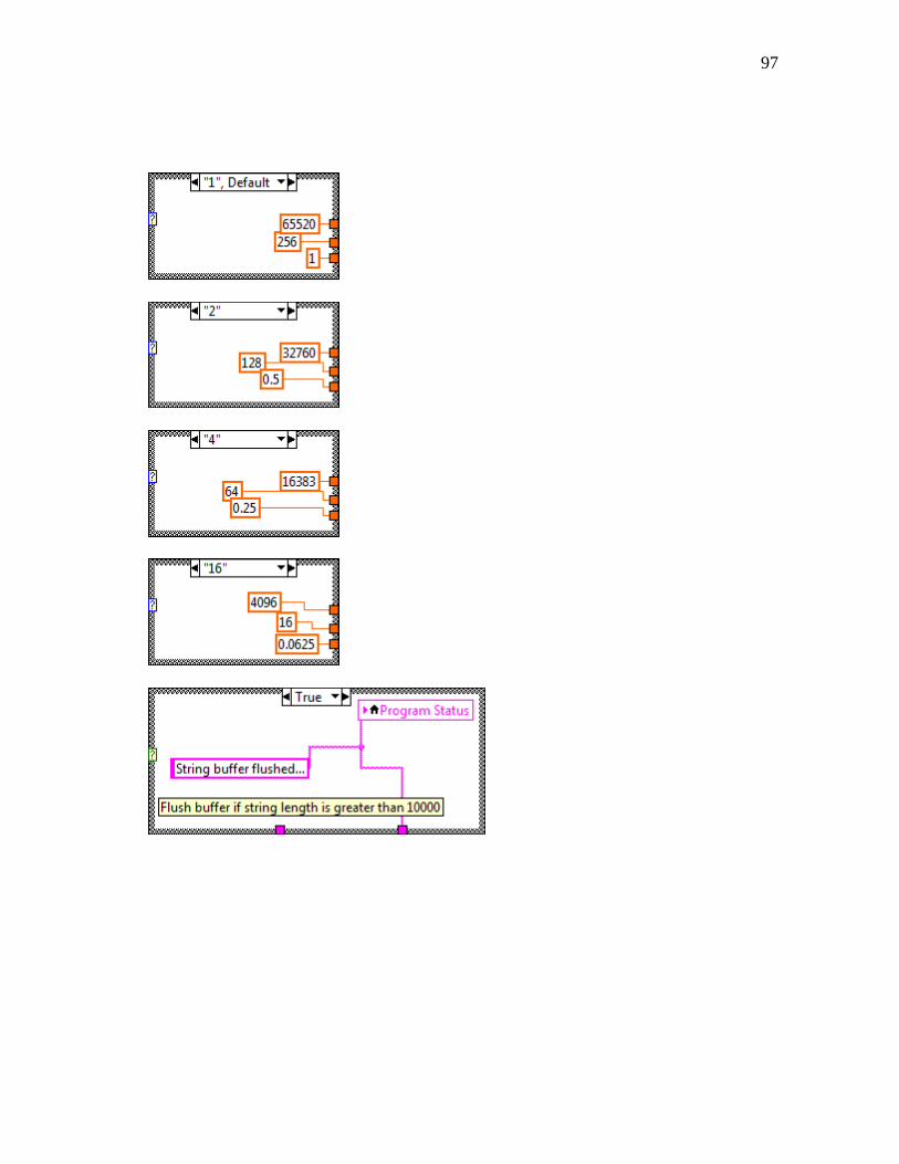
97

98

99
State S3 – Acquire Data. Pulses are collected by the counter cards within the for loop
while the pixel clock and mirror waveforms continuously generates signal. Subtraction
using a Formula Node creates actual photon count from continuously incrementing
counter card data. Counts are organized into a 2-dimensional array and displayed on-
screen. Upon completion, the laser is instructed to diverge from the sample.

100
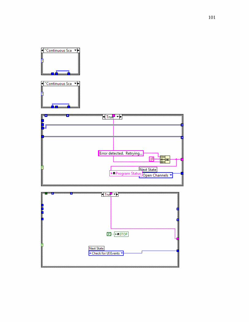
101

102

103
State S4 – Analyze Data. System checks progress on stack acquisition by an internal
counter. If an additional scan is necessary, next state is set to S2, otherwise it is set to
S5.

104

105

106

107
State S5 – Save Data. The software reads input parameters corresponding to desired file
type to be saved. The data from both channels is transferred to a sub-vi for saving, and
the on-screen indicator updates upon successful saving. If z-axis stack collection is
enabled, the stage is sent commands over USB to update stage location.

108

109

110
State S6 – Emergency Exit. Emergency stop for instantly quitting the software.
Implemented for the sake of completeness, but not used within the State Machine.

111

112
Rotate2DArray90DegreeMultiple.vi
Pre-existing VI. This VI rotates a 2D array in either clockwise or clockwise by a
multiple of 90 degrees.
Connector Pane
Front Panel

113
Block Diagram
lasershift.vi
Sub-vi used for laser divergence. Appropriate channels are initialized and activated
when divergence is desired.
Connector Pane

114
Front Panel
Block Diagram
IOMAC5000.vi
Pre-existing VI. SubVI for sending commands to the MAC5000 and receiving responses
from the MAC5000.

115
Connector Pane
Front Panel

116
Block Diagram

117
Browse_Folders.vi
Pre-existing VI. Sub-vi allows for an on-screen interface for prompting the user to select
a folder in the computer.
Connector Pane

118
Front Panel
Block Diagram
save data.vi
Sub-vi used to save collected data to the hard drive.

119
Connector Pane
Front Panel

120
Block Diagram
Property nodes are used to identify true boundaries for images. The images are exported
into the appropriate format selected by the user.
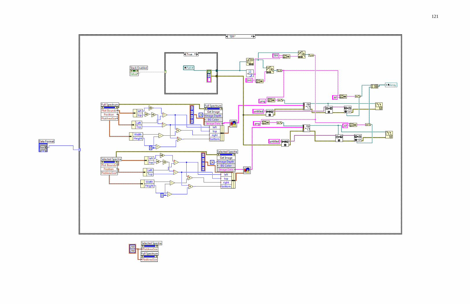
121

122

123

124

125
Waveform Buffer Generation.vi
Pre-existing VI. This subVI is used to create a Sine, Square, Triangle or Sawtooth
Waveform. The inputs to this VI are the Waveform Type, which determines if the output
waveform is a Sine, Square, Triangle, or Sawtooth Waveform, the amplitude, Desired
Frequency, Samples per Buffer, and Cycles per Buffer.
The Desired Frequency, Samples per Buffer, and Cycles per Buffer are used to calculate
the sample clock rate. The DAQmx Timing property node sets the sample clock rate for
the device specified in the task/channels in control.
The actual, coerced, sample clock rate is returned and used as an input to the Basic
Function Generator.vi. The Basic Function Generator returns a waveform of data with
timing information.
The formula below was used to determine the sample clock rate:
Desired Frequency=[(Cycles/Buffer)X(Sample Clock Rate)]/Samples per Buffer

126
Note: The Block Diagram rearranges the variables to solve for Sample Clock Rate
Connector Pane

127
Front Panel
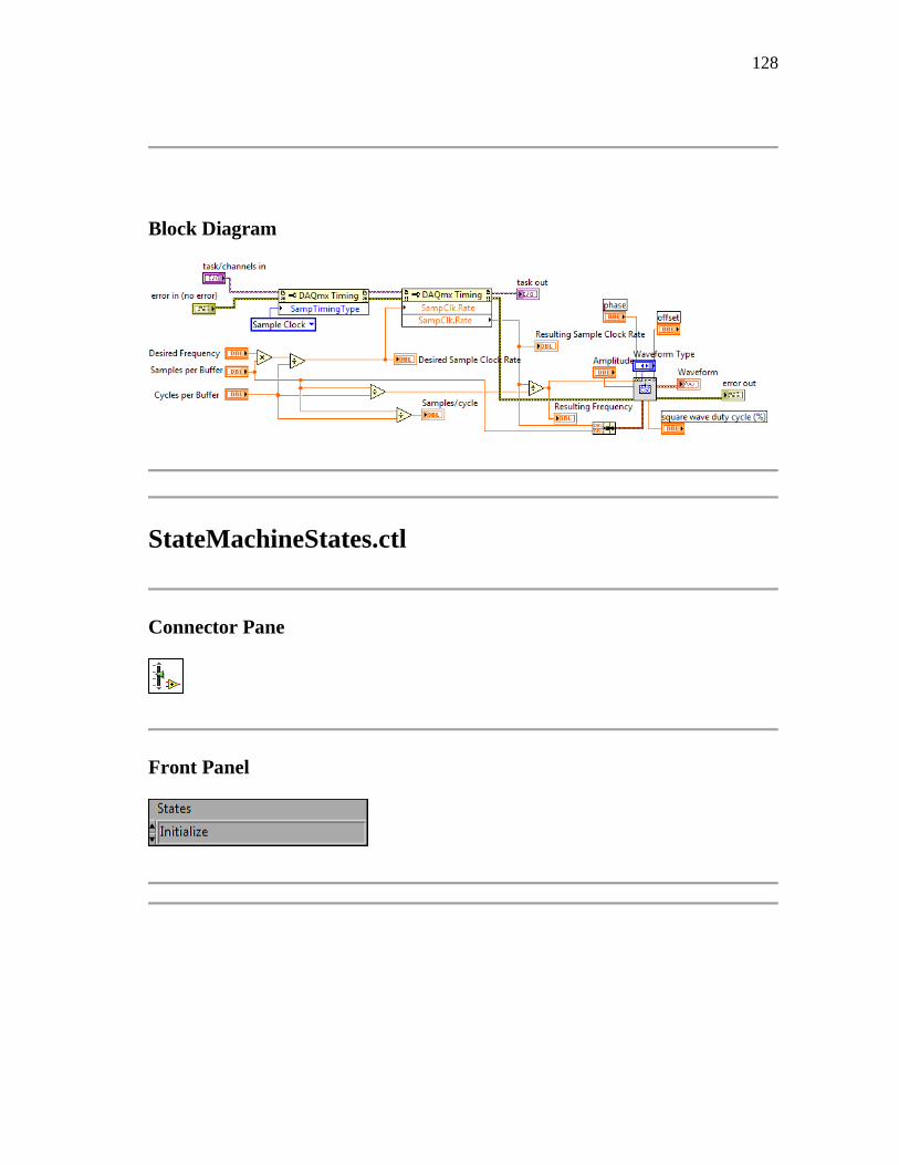
128
Block Diagram
StateMachineStates.ctl
Connector Pane
Front Panel

129
Initialization.vi
Pre-existing VI. VI initializes and configures the MAC5000; the user chooses whether
communication with the MAC5000 occurs over the Serial Port(RS232) or the USB port.
This VI should be run once at the beginning of a larger program.
Note:
Serial Port communication occurs over Serial Port 1; if the user wants to use a different
Serial Port the VISA Resource name needs to be changed in the block diagram from
ASRL1::INSTR to ASRL#::INSTR where # is the number of the Serial Port.
To use USB communication, the user needs to set up the VISA protocol using the VISA
driver development wizard. After setting up the VISA driver, the user needs to enter the
correct VISA resource name in the block diagram. Note the VISA resource name is
specific to a particular USB Bus; if the MAC5000 is plugged into another USB bus the
user needs to set up the VISA resource name again.
Connector Pane
Front Panel

130
Block Diagram

131
APPENDIX B
NOMSISV1 SOURCE CODE
Only modifications from NOMS are shown. Code not shown can be assumed to match
that of NOMS.
nomsis.vi
NOMSIS uses an updated front panel with 3 viewing panels, selectable channels, and an
on-screen spectrum.
Connector Pane

132
Front Panel

133
Block Diagram
Modification to State S2 – Initialize Channels. Code for channel activation is
replicated to activate all channels of both counter cards. Acquisition method
changed from DMA to Interrupt to prevent buffer overflow errors.

134

135
Modification to State S3 – Acquire Data. Data is acquired from all 16
channels of the counter card. Using the same code as NOMS, the code is
replicated with the only change being the corresponding channel number. The
data is compiled together as a 3-dimensional array before exiting the sub-vi.

136

137
Based on the array of channels selected on the front panel, only the active
indices of the array are pulled out and integrated together. Summed data is
then shown on-screen.

138

139
APPENDIX C
NOMSISV2 SOURCE CODE
Only modifications from NOMSISv1 are shown. Code not shown can be assumed to
match that of NOMSISv1.
Modification to State S2 – Activate Channels. Pixel clock is transferred to the FPGA via
RTSI channel. FPGA reference is opened instead of activating any counters.

140

141
FPGAread.vi
Sub-vi used to acquire and process pulses from the FPGA data stack. This sub-vi
replaces the one for data processing in NOMSISv1.
Connector Pane

142
Front Panel
Block Diagram
Acquiring data within FPGA is simplified due to the usage of a data stack. The Invoke
Node pulls data from the stack and immediately processes it into a NOMSIS 3-
dimensional array.

143

144
FPGACount16.vi
FPGACount16.vi represents the source code used for synthesis into the HDL bitfile.
Once compiled, the bitfile is stored on the hard drive and acts as a standalone
representation of the source code. The code is referenced directly by State S2.

145

146
The FPGA receives trigger signal sent over RTSI from the DAQ card. Upon activation,
the FPGA-based digital lines act as pulse counters by comparing for pulse transitions as
mentioned within the text. Upon each rising edge of the pixel clock, the current value of
the counter is stored into the FPGA data stack and reset to zero.
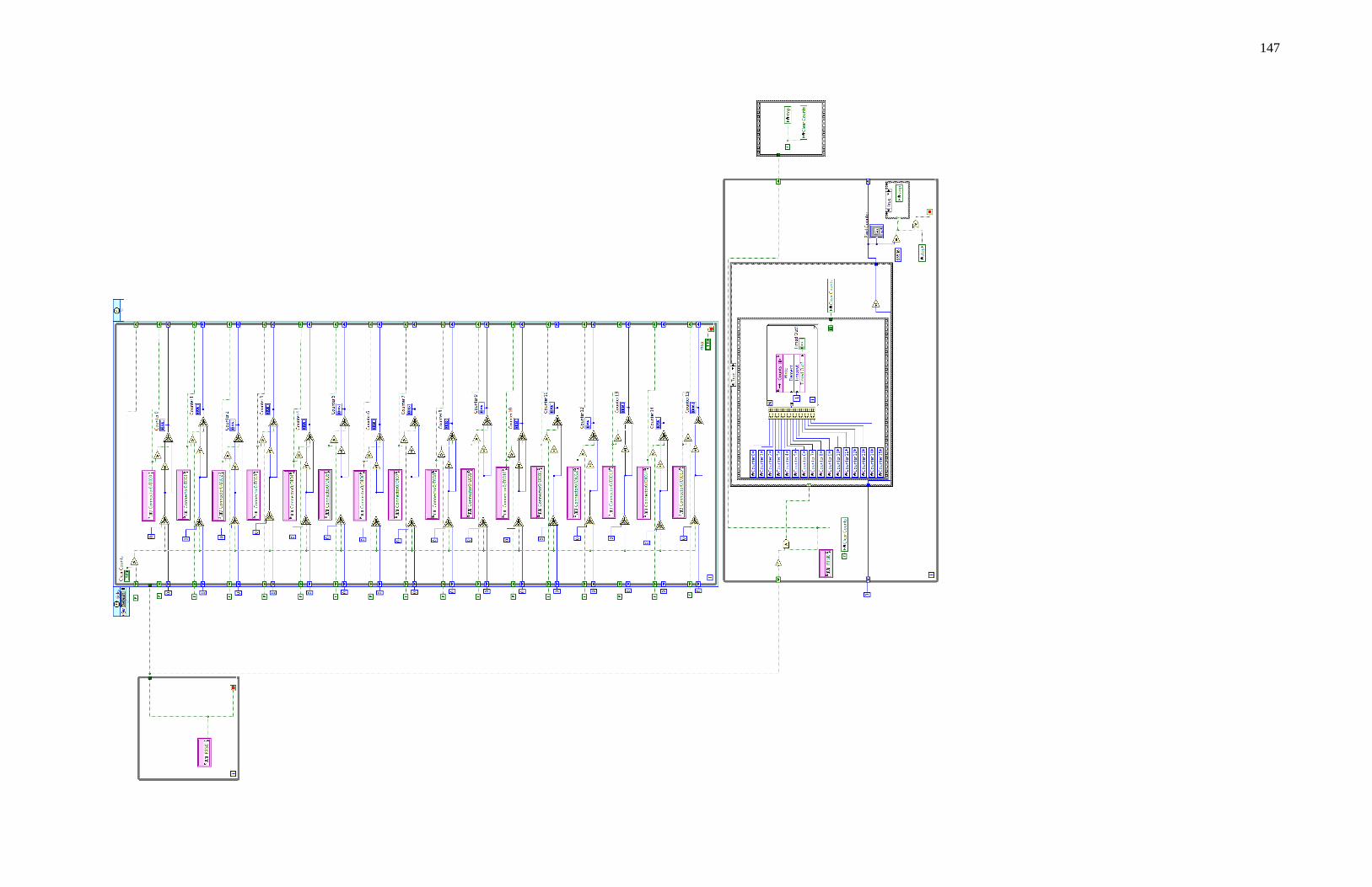
147

148

149
VITA
Anthony Chien-der Lee received his Bachelor of Science degree in electrical engineering
from The University of Texas at Austin in 2004. Shortly afterwards, he entered the
graduate program in May 2005 at Texas A&M University in College Station. He
received his Doctor of Philosophy degree in biomedical engineering in August 2011, and
will enter the Master of Business Administration program in the Mays Business School
immediately afterwards. His research interests include medical instrumentation and
imaging systems. He plans on entering the medical device industry upon completion of
his education.
Mr. Lee may be reached at 337 Zachry Engineering Center, Biomedical Engineering,
3120 TAMU, College Station, TX 77843-3120. His cellular number is 713-261-3841,
and e-mail address is [email protected].


![Generation of short pulses 2.7 fs. Ultrashort pulse generation 15 fs pulse Time [fs] Wavelength [m] Single cycle pulse](https://img.pdfslide.us/doc/110x75/56649d2b5503460f94a00e2a/generation-of-short-pulses-27-fs-ultrashort-pulse-generation-15-fs-pulse.jpg)


![Linear and nonlinear shaping of ultrashort optical pulses.scienze-como.uninsubria.it/phil/Doctorate/english/verifiche/... · Linear and nonlinear shaping of ultrashort optical pulses.]](https://img.pdfslide.us/doc/110x75/5e7c137d259a9a2cd039068a/linear-and-nonlinear-shaping-of-ultrashort-optical-linear-and-nonlinear-shaping.jpg)