Appendix B

Weight of Evidence Analysis

This page intentionally left blank

SAN JOAQUIN VALLEY PM2.5 WEIGHT OF EVIDENCE ANALYSIS

i

TABLE OF CONTENTS

EXECUTIVE SUMMARY ................................................................................................. 1

1. INTRODUCTION ...................................................................................................... 1

2. PM2.5 STANDARDS AND HEALTH EFFECTS ....................................................... 3

3. MONITORING IN THE SAN JOAQUIN VALLEY ...................................................... 4

a. Established monitoring network ......................................................................... 4

b. Extensive field studies ........................................................................................ 4

4. NATURE AND EXTENT OF THE PM2.5 PROBLEM ............................................... 7

a. Current air quality ............................................................................................... 7

b. Seasonal variability. ........................................................................................... 7

c. Diurnal variability ................................................................................................ 8

d. Chemical composition ........................................................................................ 9

e. Spatial distribution of the major PM2.5 components; local versus regional ...... 11

f. Episode development ....................................................................................... 13

5. SECONDARY AMMONIUM NITRATE FORMATION ............................................. 15

a. Chemistry ......................................................................................................... 15

b. Limiting precursor concept ............................................................................... 16

c. Role of ammonia in ammonium nitrate formation ............................................. 17

d. Role of VOC in ammonium nitrate formation .................................................... 24

6. SECONDARY ORGANIC AEROSOL FORMATION ............................................... 32

7. EMISSION SOURCES OF WINTERTIME PM2.5 ................................................... 34

a. Emission inventory ........................................................................................... 34

b. Chemical markers of source types ................................................................... 36

c. Source apportionment using source receptor models ...................................... 37

d. Photochemical modeling source apportionment ............................................... 41

8. PM2.5 AIR QUALITY PROGRESS ......................................................................... 42

a. Annual PM2.5 trends ........................................................................................ 42

b. 24-Hour PM2.5 trends ...................................................................................... 43

ii

c. Meteorology impacts on air quality ................................................................... 44

d. Annual trends adjusted for meteorology ........................................................... 47

e. 24-hour trends adjusted for meteorology ......................................................... 48

f. Trends in 24-hour, seasonal, and hourly PM2.5 ............................................... 50

g. Chemical composition trends ........................................................................... 55

h. Emission inventory trends ................................................................................ 57

9. LINKING AIR QUALITY TRENDS TO EMISSION REDUCTIONS ......................... 58

a. NOx control ...................................................................................................... 58

b. Residential wood burning controls ................................................................... 60

10. MODELED ATTAINMENT DEMONSTRATION .................................................. 62

a. Modeling results ............................................................................................... 62

b. Benefits of emission reductions from on-going programs ................................ 63

c. Evaluation of precursor sensitivity .................................................................... 64

d. Demonstrating attainment at Bakersfield-California ......................................... 70

11. SUMMARY .......................................................................................................... 71

REFERENCES .............................................................................................................. 72

APPENDIX 1

APPENDIX 2

APPENDIX 3

APPENDIX 4

E-1

EXECUTIVE SUMMARY

The San Joaquin Valley 2012 PM2.5 Plan demonstrates that the San Joaquin Valley will attain the PM2.5 24-hour standard of 35 ug/m3 as expeditiously as practicable due to adopted and proposed control measures. As part of the attainment demonstration, the 2012 PM2.5 Plan specifically identifies the: 1) most expeditious date of when the San Joaquin Valley (Valley) will attain the standard, 2) attainment plan precursors, 3) amount of emissions needed to attain, and 4) sources to control. The weight of evidence analysis provides a set of complementary analyses that supplement the required modeling. Because all methods have strengths and weaknesses, examining an air quality problem in a variety of ways offsets the limitations and uncertainty that are inherent in air quality modeling. This approach also provides a better understanding of the overall problem and the level and mix of emissions controls needed for attainment. Analyses conducted by Air Resources Board (ARB) and San Joaquin Valley Air Pollution Control District (SJVAPCD or District) staff, along with findings from the California Regional Particulate Air Quality Study (CRPAQS) provide the supplemental information supporting the attainment demonstration. CRPAQS was a public/private partnership designed to advance our understanding of the nature of PM2.5 in the Valley and guide development of effective control strategies. The study included monitoring at over 100 sites as well as data analysis and modeling, results of which have been published in over 60 papers and presented at national and international conferences. Studies such as CRPAQS provide valuable information that supports the State Implementation Plan (SIP) process in a number of ways. First, these studies provide additional observational data that help to provide a more detailed understanding of the nature of the PM2.5 problem in the San Joaquin Valley. This data also is used to update the fundamental algorithms contained within air quality models, thereby enhancing their ability to simulate observed air quality conditions. Finally, they provide an improved basis for model applications used in the preparation of SIPs and a more robust platform for evaluating the response to emission controls and predicting future air quality. What is the nature of the 24-hour PM2.5 problem in the Valley? The geography of the San Joaquin Valley, along with weather patterns influence the accumulation, formation, and dispersion of PM2.5. As a result, PM2.5 concentrations are generally higher in the central and southern portions of the Valley, with highest values in the urban areas of Fresno and Bakersfield. Concentrations are highest during the winter months of November through February. During these months, high-pressure weather systems over Northern California can cause the atmosphere to become stagnant for extended periods, resulting in PM2.5 episodes that can persist from several days up to several weeks. Ammonium nitrate and carbonaceous material (organic and elemental carbon) are the largest constituents of PM2.5 on exceedance days, comprising 85 to 90 percent of the

E-2

mass. Geological material (dust), and ammonium sulfate are small contributors. Ammonium nitrate is formed in the atmosphere from reactions of gaseous precursors. Emissions of nitrogen oxides (NOx) from mobile sources and stationary sources react with ammonia which is primarily emitted from livestock operations, fertilizer application, and mobile sources. The stagnant, cold, and damp conditions that occur during the winter promote the formation and accumulation of ammonium nitrate. Elevated concentrations can be found at both urban and rural sites. In contrast, organic carbon is highest in urban areas due to emissions from residential wood combustion, commercial cooking operations, and mobile source tailpipe emissions which are largest in urban areas. Due to the localized urban increment from these activities, which adds to the more regional ammonium nitrate concentrations, the highest PM2.5 concentrations in the Valley occur at urban sites. What progress has been made in reducing PM2.5 concentrations?

The Valley has experienced progress in reducing both annual average and 24-hour PM2.5 concentrations over the last ten years. Between 2001 and 2011, annual average design values in the Valley declined between 30 and 40 percent at individual monitoring locations. Overall, annual PM2.5 trends adjusted for the effects of meteorology indicate that between 1999 and 2010, annual PM2.5 concentrations decreased about 40 to 50 percent at Bakersfield and Fresno due to emission reductions. With on-going implementation of the 2008 PM2.5 Plan, annual average PM2.5 concentrations in the Valley are expected to continue to improve and reach attainment in 2014.

During this same time period, 24-hour PM2.5 design values in the Valley have also decreased between approximately 30 and 50 percent. In addition, the number of days exceeding the 24-hour standard decreased by about 45 to 50 percent. After adjusting for the influence of meteorology, the number of exceedance days has decreased between 60 and 65 percent in Bakersfield and Fresno.

Additional evaluations provide further insight into the annual and 24-hour PM2.5 progress that has been observed. For example, as the fraction of days recording PM2.5 levels above the 24-hour standard has decreased, there has been a corresponding increase in the fraction of days below the level of the annual standard of 15 ug/m3. Average concentrations during the winter months have decreased, and under similar meteorological conditions, peak 24-hour concentrations during episodes are now 40 percent lower than they were ten years ago. What are the attainment plan precursors? Ambient PM2.5 is comprised of many different constituents and as a result there are multiple precursor pollutants that lead to PM2.5 formation (directly emitted PM2.5, NOx, sulfur oxides (SOx), volatile organic compounds (VOCs), and ammonia). The U.S. Environmental Protection Agency’s (U.S. EPA) PM2.5 implementation rule specifies that a precursor is considered “significant” for control strategy development purposes when a significant reduction in the emissions of that precursor pollutant leads to a significant decrease in PM2.5 concentrations. Such pollutants are known as

E-3

“PM2.5 attainment plan precursors” (72 FR 20586). The PM2.5 implementation rule also establishes a presumption that PM2.5, NOx, and SOx are attainment plan precursors, while VOCs and ammonia are not. For the annual PM2.5 plan, PM2.5, NOx, and SOx were identified and approved as the only attainment plan precursors by U.S. EPA. Given the large contribution of ammonium nitrate on 24-hour PM2.5 exceedance days, a number of different studies and analyses were evaluated to understand the role of VOCs and ammonia in ammonium nitrate formation in the San Joaquin Valley and to determine whether they should be considered attainment plan precursors for the 2012 24-hour PM2.5 Plan. The amount of ammonium nitrate produced depends upon the relative atmospheric abundance of its precursors. It is therefore important to understand which precursor controls are most effective in reducing ammonium nitrate concentrations. In simple terms, the precursor in shortest supply will limit how much ammonium nitrate is produced. This is known as the limiting precursor and controls of this precursor will have the most significant benefits in reducing PM2.5 concentrations. The precursor assessment for the 24-hour PM2.5 plan included evaluation of emissions inventories, monitoring studies, and photochemical modeling analyses of ammonium nitrate sensitivity to precursor emission reductions. While emissions inventory and monitoring data can indicate the relative abundance of the different precursors, photochemical models provide a quantitative approach to simulate the effects that emission reductions in each of gaseous precursors would have on the predicted ammonium nitrate concentrations. Evaluation of both emissions inventory and monitoring data concluded that the ammonia-rich conditions throughout the Valley demonstrate that NOx rather than ammonia is the limiting precursor during wintertime PM2.5 episodes. In addition, photochemical modeling studies found that while large reductions in NOx led to commensurate reductions in ammonium nitrate, comparable reductions in ammonia were much less effective. Precursor sensitivity modeling conducted for the 2012 PM2.5 Plan showed that on a per ton basis, reductions in NOx are approximately nine times more effective than reductions in ammonia. Finally, evaluation of ambient air quality trends show that reductions in NOx emissions, gaseous NOx concentrations, and particulate nitrate all track each other well. Evaluation of monitoring studies also provided some evidence that VOCs could be important at times, however these studies were not conclusive. Therefore photochemical modeling studies are more appropriate to assess the overall impact of VOC controls. These modeling studies found that at current NOx levels, further VOC emission reductions produce essentially no benefit, and in some instances may actually lead to an increase in ammonium nitrate concentrations. Findings from these prior studies were supported by precursor sensitivity modeling conducted for the 2012 PM2.5 SIP, which indicated a very small disbenefit from reductions in VOCs.

E-4

As noted previously, U.S. EPA’s PM2.5 implementation rule directs SIP planning efforts and regulation to those pollutants generally known to significantly contribute to PM2.5 concentrations. Based on the weight of evidence presented from historical studies, coupled with the modeled precursor sensitivity analyses conducted as part of the 2012 PM2.5 Plan, VOCs and ammonia are not considered significant precursors for 24-hour PM2.5. Therefore the 2012 24-hour PM2.5 plan attainment precursors are directly emitted PM2.5, NOx, and SOx. When will the Valley attain the 24-hour PM2.5 standard? Consistent with U.S. EPA guidelines, air quality modeling was done to predict future PM2.5 concentrations at each monitoring site in the San Joaquin Valley. This modeling shows attainment of the 24-hour PM2.5 standard by 2019 in all counties except Kings and Kern, based on implementation of the ongoing control program. In these counties, additional focused emission reductions are needed to provide for attainment. The modeling analysis includes new emission reductions each year between now and 2019 from implementation of a combination of adopted ARB and District programs. As a result, most sites in the northern and central Valley are expected to attain prior to 2019. ARB staff then modeled a scenario with an enhanced wood burning curtailment program Valley wide, which would be designed to prevent wood burning on days that may lead up to a PM2.5 exceedance. The predicted design values for each site from this modeling scenario are shown in Table E-1.

Table E-1.

2019 Modeled 24-hour PM2.5 Design Values with Enhanced Residential Wood Burning Curtailment Program.

Monitoring Site Design Value (µg/m3) Bakersfield - California 35.7 Bakersfield - Planz 32.9 Corcoran - Patterson 32.1 Visalia - N. Church 29.4 Fresno - Hamilton 28.6 Fresno - First 30.5 Clovis 28.6 Merced 22.6 Modesto 24.7 Stockton 21.4 While adoption of a more stringent wood burning curtailment program brings the Bakersfield-California site very near attainment, further reductions are still needed and will be provided through a measure to achieve additional emission reductions from commercial cooking operations. Design values at all other sites are well below attainment levels.

E-5

What is the attainment control strategy?

In order to determine the emission reductions needed to bring Bakersfield into attainment, ARB staff conducted additional modeling sensitivity runs to assess the relative efficacy of further reductions of different PM2.5 precursors. The current 24-hour PM2.5 standard modeling demonstrates that on a relative basis the greatest benefits are achieved from reductions in sources of directly emitted PM2.5, followed by NOx, based on U.S. EPA’s relative response factor procedures. Kern County specific model sensitivity runs were also conducted to evaluate the benefits of emission reductions focused on the Bakersfield area. These runs show that directly emitted PM2.5 emission reductions are approximately 8 times more effective than NOx reductions. The implementation of new reductions from California’s on-going emission control programs will provide the majority of the emission reductions needed to attain the 24-hour PM2.5 standard throughout the San Joaquin Valley in 2019. The PM2.5 design value at the Bakersfield-California site must decrease by approximately 45 percent to demonstrate attainment. Between 2007, the base year used in the photochemical modeling attainment demonstration and 2019, implementation of these control programs will reduce NOx emissions by 55 percent. The weight of evidence analysis has demonstrated that prior reductions in NOx have resulted in commensurate reductions in ambient concentrations of nitrate. This is consistent with modeled predictions that demonstrate a nearly 50 percent reduction in ammonium nitrate concentrations. In addition, while directly emitted PM2.5 emissions in aggregate are decreasing by nearly 30 percent, a major focus of the attainment control strategy is further curtailment of residential wood burning, along with implementation of a measure to reduce emissions from commercial cooking. District analysis has demonstrated the significant benefits of past implementation of wood burning curtailment. Further, examination of emission sources surrounding the Bakersfield-California monitor, and a modeling sensitivity run support the benefits of reducing emissions from cooking operations. The final attainment demonstration for the Bakersfield-California design site is provided in Table E-2.

E-6

Table E-2.

Attainment Demonstration for the Bakersfield-California Design Value Site.

2007 Design Value (ug/m3)

2019 Design Value with Wood

Burning Program Enhancement

(ug/m3)

2019 Final Design Value (ug/m3)

65.6 35.7 ≤35.4 Note: The benchmark for attainment is a design value that is equal to

or less than 35.4 µg/m3.

Consideration of the entirety of information presented in the weight of evidence provides a consistent assessment that supports the modeled attainment date of 2019. The substantial continuing reductions that will result from implementation of the ongoing control program, coupled with new measures addressing residential wood burning and cooking, are consistent with the results predicted in the modeled attainment demonstration.

1

1. INTRODUCTION

The 2012 PM2.5 Plan demonstrates that the San Joaquin Valley will attain the PM2.5 24-hour standard as expeditiously as practicable due to adopted and proposed control measures. As part of the attainment demonstration, the 2012 PM2.5 Plan specifically identifies the: 1) most expeditious date for when the San Joaquin Valley (SJV or Valley) will attain the standard, 2) attainment plan precursors, 3) amount of emissions needed to attain, and 4) sources to control. Following U.S. Environmental Protection Agency (U.S. EPA) guidance and procedures, the attainment demonstration was conducted through a modeled attainment test. Photochemical modeling was used to identify the most expeditious attainment date, the relative benefits of controlling different PM2.5 precursor pollutants, and the magnitude of emission reductions needed from each pollutant. The Weight of Evidence (WOE) analysis provides a set of complementary analyses that supplement the required modeling.

A WOE approach looks at the entirety of the information at hand to provide a more informed basis for the attainment strategy. Because all methods have strengths and weaknesses, examining an air quality problem in a variety of ways offsets the limitations and uncertainty that are inherent in air quality modeling. This approach also provides a better understanding of the overall problem and the level and mix of emissions controls needed for attainment. The U.S. EPA recognizes the importance of a comprehensive assessment of air quality data and modeling and encourages this type of broad assessment for all attainment demonstrations. In their modeling guidance, they further note that the results of supplementary analyses may be used in a WOE determination to show that attainment is likely despite modeled results which may be inconclusive (U.S. EPA 2007). Following the U.S. EPA guidance, future year modeled 24-hour design values that fall between 32 and 37 ug/m3 need to be accompanied by a WOE demonstration to determine whether attainment will occur. This range in modeled design values reflects the uncertainty in predicting absolute PM2.5 concentrations that is inherent in air quality modeling, and therefore recognizes that an improved assessment of attainment can be derived from examining a broader set of analyses. U.S. EPA recommends that three basic types of analyses be included to supplement the primary modeling analysis in the WOE approach: 1) analyses of trends in ambient air quality and emissions, 2) observational models and diagnostic analyses, and 3) additional modeling evaluations. The scope of the WOE analysis is different for each nonattainment area. The level of detail appropriate for each area depends upon the complexity of the air quality problem, how far into the future the attainment deadline is, and the amount of data and modeling available. For example, less analysis is needed for an area that is projecting attainment near-term and by a wide margin, and for which recent air quality trends have demonstrated significant progress, than for areas with more severe air quality challenges

2

The following sections present the WOE assessment that supports the attainment demonstration the 24-hour PM2.5 standard in the San Joaquin Valley.

3

2. PM2.5 STANDARDS AND HEALTH EFFECTS PM2.5 is a complex mixture of particles and liquid droplets that vary in size and chemical composition. As a subset of PM10, particles with diameters up to 10 micrometers, PM2.5 comprises particles with diameters up to 2.5 micrometers (Figure 1). PM2.5 contains a diverse set of substances including elements such as carbon and metals, compounds such as nitrates, sulfates, and organic materials, and complex mixtures such as diesel exhaust and soil or dust. Some of the particles are directly emitted into the atmosphere. Others, referred to as secondary particles, result when gases are transformed into particles through physical and chemical processes in the atmosphere. Figure 1. PM2.5 particle diameter compared to the thickness of a single strand of hair.

Numerous health effects studies have linked exposure to PM2.5 to increased severity of asthma attacks, development of chronic bronchitis, decreased lung function in children, increased respiratory and cardiovascular hospitalizations, and even premature death in people with existing cardiac or respiratory disease. In addition, California has identified particulate exhaust from diesel engines as a toxic air contaminant – suspected to cause cancer, other serious illnesses, and premature death. Those most sensitive to PM2.5 pollution include people with existing respiratory and cardiac problems, children, and older adults. Ambient air quality standards establish the levels above which PM2.5 may cause adverse health effects. In 1997, U.S. EPA adopted the first set of PM2.5 air quality standards, an annual standard of 15 µg/m3 and a 24-hour standard of 65 µg/m3. To address the 1997 PM2.5 standards, the San Joaquin Valley Air Pollution Control District (SJVAPCD or District) adopted the 2008 PM2.5 Plan. At the time of plan development, the San Joaquin Valley already attained the 24-hour standard, thus the 2008 PM2.5 Plan focused on the annual PM2.5 standard. U.S. EPA approved this Plan in 2011 (76 FR 41338; 76 FR 69896). In 2006, U.S. EPA tightened the 24-hour standard to 35 µg/m3. Attainment of this standard is the focus of the SJV 2012 PM2.5 Plan.

4

3. MONITORING IN THE SAN JOAQUIN VALLEY

a. Established monitoring network An extensive network of PM2.5 monitors throughout the SJV provides data to assess compliance with ambient air quality standards and to study the nature of ambient PM2.5. Currently, the network comprises 21 monitoring sites. Many sites include multiple monitoring instruments running in parallel. Seven sites operate Federal Reference Monitors (FRMs), which provide regulatory data that are used to assess compliance with the federal PM2.5 standards. An additional 20 monitors provide hourly PM2.5 measurements. Eleven of these continuous monitors are Federal Equivalent Monitors (FEM), which can also be used to assess compliance with the standards. The FRM and FEM monitoring sites are shown in Figure 2. The locations of these monitors are designed to capture population exposure. In addition, data collected at these monitors serve to report air quality conditions to the public, and support forecasting for the District’s agricultural and residential burning curtailment programs. Finally, four sites have chemical speciation monitors. The speciation monitors collect samples that are further analyzed in the laboratory to determine the chemical make-up of PM2.5. Figure 2. San Joaquin Valley PM2.5 monitoring network (FRMs and FEMs, October 2012).

b. Extensive field studies The San Joaquin Valley is one of the most studied areas in the world with an extensive number of publications in peer-reviewed international scientific/technical journals and other major reports. Since 1970, close to 20 major field studies have been conducted in the Valley and surrounding areas that have elucidated various aspects of the nature and

5

causes of ozone and particulate matter. A comprehensive listing of publications (reports and peer-reviewed journal articles) is provided in Appendix 1. The first major study specifically focused on particulate matter was the Integrated Monitoring Study in 1995 (IMS-95), which was the pilot study for the subsequent California Regional Particulates Air Quality Study (CRPAQS) in 2000 (Solomon and Magliano, 1998). IMS-95 formed the technical basis for the SJV 2003 PM10 Plan that was approved by the U.S. EPA in 2004 (71 FR 63642), and the Valley was subsequently re-designated as attainment in 2008 (73 FR 66759). CRPAQS was a key component of the technical foundation for the SJV 2008 PM2.5 Plan that U.S. EPA approved in 2011 (76 FR 41338; 76 FR 69896). Although conducted more than ten years ago, CRPAQS findings remain relevant to the development of the current 24-hour PM2.5 Plan. CRPAQS was a public/private partnership designed to advance the understanding of the nature of PM2.5 in the Valley and guide development of effective control strategies. The study included monitoring at over 100 sites (Figure 3) as well as data analysis and modeling, results of which have been published in over 60 papers and presented at national and international conferences. The field campaign was carried out between December 1999 and February 2001. CRPAQS improved our understanding of the spatial and temporal distribution of PM2.5 in the Valley, its chemical composition, transport and transformation processes, and contributing sources. More details on CRPAQS can be found at the following link: http://www.arb.ca.gov/airways/ccaqs.htm.

Figure 3. CRPAQS monitoring program.

Findings from CRPAQS and other studies have been integrated into the conceptual model of PM2.5 in the San Joaquin Valley. The conceptual model provides the scientific foundation for the WOE analysis supporting the 24-hour PM2.5 standard attainment demonstration. Specific findings are integrated into the various WOE analysis sections of this document.

6

Further field studies relevant to PM2.5 include the California portion of the Arctic Research of the Composition of the Troposphere (ARCTAS-CARB) which took place in 2008 (Jacob, et al., 2010) and Research at the Nexus of Air Quality and Climate (CalNex2010) conducted in 2010 (www.esrl.noaa.gov/csd/calnex/). The monitoring operations for both studies occurred during the early to mid-summer and extended over Southern California and the Central Valley. Some study findings have been published (e.g., Kaduwela and Cai, 2009, Cai and Kaduwela, 2011, Kelly et al., 2011), but data analysis is still in progress.

7

4. NATURE AND EXTENT OF THE PM2.5 PROBLEM

a. Current air quality The geography of the San Joaquin Valley, along with large-scale regional and local weather patterns, influence the accumulation, formation and, dispersion of air pollutants. Covering nearly 25,000 square miles, the Valley is a lowland area bordered by the Sierra Nevada Mountains to the east, the Pacific Coast range to the west, and the Tehachapi Mountains to the south. The mountains act as air flow barriers, with the resulting stagnant conditions favoring the accumulation of pollutants. To the north, the Valley borders the Sacramento Valley and Delta lowland, which allows for some level of pollutant dispersion. As a result of geography and meteorology, PM2.5 concentrations are generally higher in the southern and central portions of the Valley. To determine attainment for the 24-hour standard, the design value at each monitoring site must be calculated following strict U.S.EPA protocols. The design value represents a three-year average of the 98th percentile of the measured PM2.5 concentrations. Depending on a site’s 24-hour PM2.5 data collection schedule, the 98th percentile usually corresponds to a value between the 2nd and the 8th highest value. If the design value is equal to or below 35.4 μg/m3, the site attains the standard. Figure 4 shows the 2011 24-hour PM2.5 design values throughout the San Joaquin Valley. All sites currently record design values above the standard, although design values are generally lower in the northern and central Valley. Urban sites in the Fresno and Bakersfield areas register the higher design values. Figure 4. 2011 24-hour design values

b. Seasonal variability PM2.5 concentrations in the San Joaquin Valley exhibit a strong seasonal pattern, with highest concentrations occurring from November through February (Figure 5). During the winter, PM2.5 builds up over several days or weeks. These PM2.5 episodes are caused by increased activity in some emission sources and by meteorological

010203040506070

PM2.

5 De

sign

Val

ue (µ

g/m

3 )

2011 24-Hour PM2.5 Design Values

Standard

8

conditions that are conducive to the build-up and formation of PM2.5. During the winter, high-pressure weather systems over California can cause the atmosphere to become stagnant for extended periods leading to temperature inversions. Under normal conditions, temperature decreases with altitude, allowing free upward air flow and dispersing emissions and pollutants. In contrast, a temperature inversion positions a layer of warmer air above cooler air, impeding upward flow of emissions and air pollutants. Often the inversion layer is lower than the mountains surrounding the Valley, trapping emissions and pollutants. Figure 5. Seasonal variation in PM2.5 concentrations at Bakersfield-California.

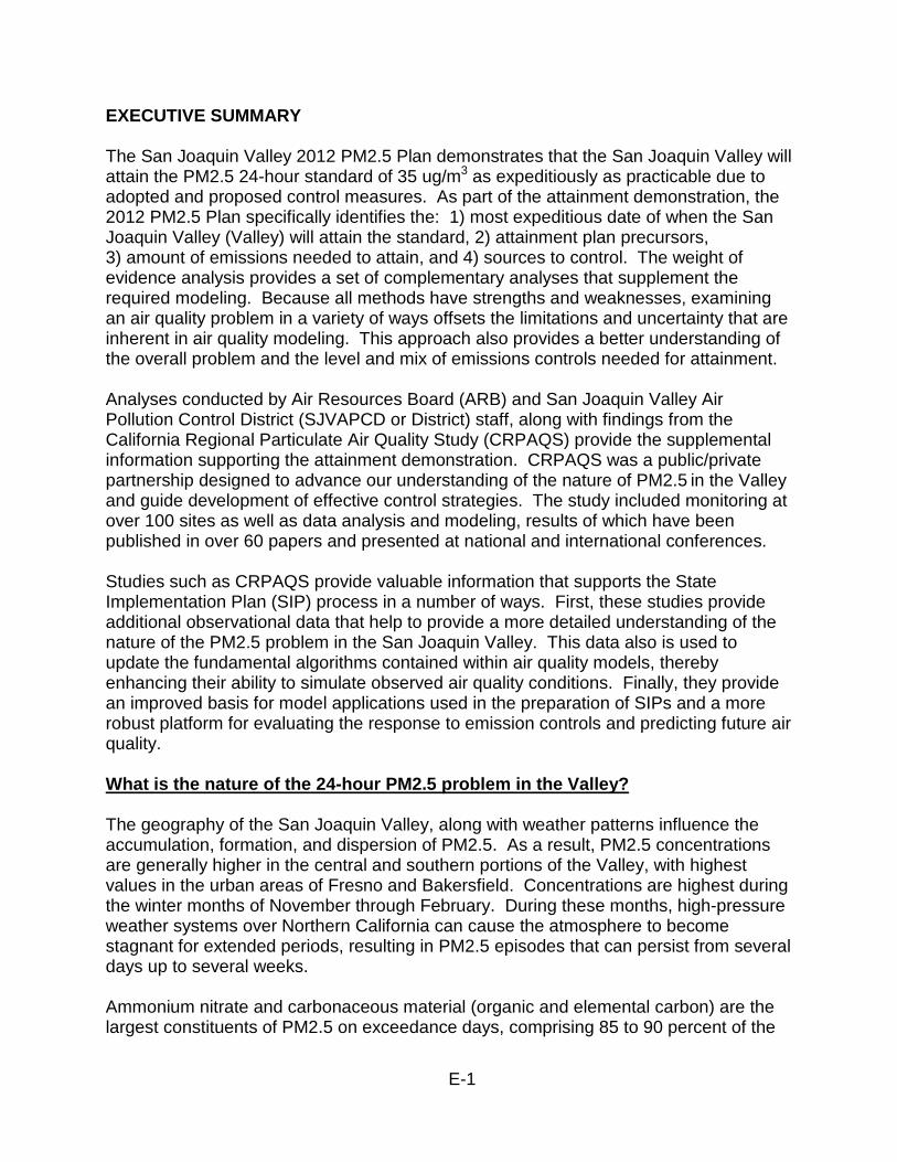
c. Diurnal variability During the winter, PM2.5 levels in the San Joaquin Valley also vary significantly across the 24-hour period. For example, in urban Fresno, the highest PM2.5 concentrations occur during the night (Figure 6). Peak evening concentrations generally reflect the influence of lowering inversion heights which trap pollutants close to the surface, as well as increased activity from evening commute traffic and residential wood combustion. The smaller peak of PM2.5 concentrations observed during mid-day is due in part to traffic activity, but mostly reflects secondary pollutant formation and PM2.5 formed above the inversion layer from previous day’s emissions that mix back to the surface during the day.

0

10

20

30

40

50

1 2 3 4 5 6 7 8 9 10 11 12

Con

cent

ratio

n (µ

g/m

3)

Month

2009-2011 Monthly Average PM2.5 Concentration at Bakersfield-California

9

Figure 6. Variation in hourly PM2.5 concentrations during the winter at Fresno-1st.

d. Chemical composition Examination of the chemical make-up of PM2.5 on days exceeding the daily standard provides another important element in understanding the nature of PM2.5 in the Valley and contributing sources. The pie charts in Figure 7 show the current chemical components that contribute to PM2.5 on days that exceed the standard at urban sites in the southern (Bakersfield), central (Fresno), and northern (Modesto) regions of the Valley. These sites currently record the highest PM2.5 concentrations in their corresponding regions. While the relative percentages vary, in all cases the major components are ammonium nitrate and organic material (organic carbon). Ammonium nitrate is the largest contributor to PM2.5, especially in the southern region. At Bakersfield, ammonium nitrate constitutes about 65 percent of PM2.5, while at Fresno and Modesto it constitutes about 55 percent. Ammonium nitrate is formed in the atmosphere from chemical reactions of NOx and ammonia. Sources emitting NOx include motor vehicles and stationary combustion sources. The largest sources of ammonia are livestock operations, fertilizer application, and mobile. The stagnant, cold, and damp conditions that occur during the winter promote the formation and accumulation of ammonium nitrate. Additional information on ammonium nitrate formation can be found in section 5. The organic matter component of PM2.5 is largest in the central and northern portions of the Valley. Organic matter constitutes about 30 percent of PM2.5 at Modesto and Fresno compared to less than 20 percent at Bakersfield. Activities such as residential wood combustion, cooking, biomass burning, and direct tailpipe emissions from mobile sources contribute to the PM2.5 organic matter component. Ammonium sulfate and elemental carbon each contribute about five percent at the three sites. Ammonium sulfate is also formed in the atmosphere from SOx emitted from

0

10

20

30

40

50

0 4 8 12 16 20PM2.

5 C

once

ntra

tion

(μg/

m3 )

Time-of-day

2009-20011 Average Hourly PM2.5 Variation During Nov-Dec at Fresno-1st

2009-2011

10

combustion sources. Elemental carbon results from mobile and stationary combustion sources, with significant contributions from diesel sources. Geological material contributes to a lesser extent, about five percent at Bakersfield and about two percent at Modesto and Fresno. Geological material comes from dust suspended into the air by vehicle travel on roads, soil from agricultural activities, and other dust producing activities such as construction. Figure 7. 2009-2011 average peak day PM2.5 chemical composition at a) Bakersfield, b) Fresno, and c) Modesto.

Ammon. Nitrate 65%

Ammon. Sulfate

7%

Organic Matter 17%

ElementalCarbon

5%

Geologic. 5%

Elements 1%

a) 2009-2011 Peak Day PM2.5 Composition at Bakersfield

Ammon. Nitrate 54%

Ammon. Sulfate

6%

Organic Matter 29%

Elemental Carbon

6%

Geologic. 2%

Elements 3%

b) 2009-2011 Peak Day PM2.5 Composition at Fresno-1st

Ammon. Nitrate 56%

Ammon. Sulfate

6%

Organic Material

28%

ElementalCarbon

6%

Geologic. 2%

Elements 2%

c) 2009-2011 Peak Day PM2.5 Composition at Modesto

11

e. Spatial distribution of the major PM2.5 components; local versus regional

As noted previously, high PM2.5 concentrations in the Valley occur almost exclusively during multiday pollution episodes under stagnant winter weather conditions. The duration and strength of an episode depends on atmospheric stability, but episodes can last several weeks. Once the weather conditions conducive to an episode set in, PM2.5 concentrations increase due to the accumulation of primary pollutants and formation of secondary pollutants.

Each episode has a regional as well as local component (Turkiewicz et al., 2006). High concentrations of nitrate can occur over large regions, including both urban and rural areas (Figure 8). As shown in Figure 9, ammonia is mostly concentrated in rural areas, particularly between Fresno and Bakersfield. On the other hand, high concentrations of organic carbon are more localized around urban sites, especially Fresno, with lower concentrations at rural sites (Figure 10).

The differences between the regional and local component can be traced back to the emission sources and subsequent formation and transport processes for each chemical component. Gaseous precursors of ammonium nitrate (NOx and ammonia) are transported much more efficiently than directly emitted organic matter particles (Ying and Kleeman, 2009). Although, some of the emitted NOx forms ammonium nitrate in urban areas, it is also transported to downwind regions where it reacts with ammonia to form particulate ammonium nitrate in the rural areas. While transport does occur, the distances are still relatively limited, with transport distances of 50 to 60 kilometers in the central and southern Valley. Ying et.al. (2009) found for example that most of the PM2.5 nitrate in Bakersfield is produced from sources within the southern Valley.

In contrast, carbonaceous aerosols are emitted into the atmosphere as particles and have a shorter lifetime due to higher deposition rates. Under stagnant conditions they can only be transported a short distance and therefore, have the greatest impact locally. Transport distances for carbonaceous aerosols during CRPAQS were only 20 to 40 kilometers. Due to this localized organic carbon increment, which adds to the more regional ammonium nitrate concentrations, the highest PM2.5 concentrations occur at urban sites.

12

Figure 9. Spatial distribution of annual ammonia (NH3) concentrations (2/1/2000-1/31/2001) during CRPAQS (Chow et al., 2005).

Figure 8. Spatial distribution of winter ammonium nitrate concentrations measured during CRPAQS (Chow et al., 2005).

13

f. Episode development The development of PM2.5 episodes in the Valley is strongly controlled by meteorological conditions. The rate of concentration buildup depends on the intensity of atmospheric stability, with concentrations building up faster at urban sites than at rural sites (Turkiewicz et al., 2006). Figure 11 illustrates the differences in the PM2.5 buildup rate between an urban (Fresno) and a rural (Selma) site in the Fresno area during CRPAQS. Although urban sites reach the highest overall concentrations, at the end of an episode rural sites may reach equivalent levels. However, because of the lag in the overall buildup rate, rural sites have fewer days above the standard and lower episode-average concentrations.

Figure 11. Atmospheric stability and buildup of PM2.5 concentrations at an urban site (Fresno) and a rural site (Selma) in the Fresno area during the December 2000 CRPAQS episode.

-5

0

5

10

15

20

020406080

100120140160

12/19/00 12/22/00 12/25/00 12/28/00 12/31/00 1/3/01 1/6/01 Stab

ility

(T85

0-Tm

in °C

)

PM2.

5 M

ass

(µg/

m3 )

Episode Day

Fresno PM2.5 Selma PM2.5 Stability

Figure 10. Spatial distribution of winter organic carbon concentration measured during CRPAQS (Chow et al., 2005).

14

The rate of buildup and the differences between urban and rural sites can be explained by the differential contributions of ammonium nitrate and organic carbon. Throughout the duration of an episode, ammonium nitrate concentrations tend to build to a plateau that is maintained until a weather front breaks the stagnation, causing the levels to decrease. Figure 12 illustrates the buildup of ammonium nitrate concentrations measured during the 2000/2001 PM2.5 episode in Bakersfield. This ammonium nitrate buildup generally begins in urban areas, followed by a buildup in rural areas as urban NOx is mixed downwind and reacts with rural ammonia. In contrast, organic carbon is largest in urban areas, and tends to be more stable across an episode, although individual peaks can occur during periods of enhanced wood burning such as weekends and holidays. The combination of early ammonium nitrate buildup along with the urban organic carbon increment results in the highest concentrations being observed in urban areas. The abrupt decrease in concentrations on January 8th was due to the passage of a cold front effectively ending the PM2.5 episode.

Figure 12. Ammonium nitrate concentrations at Bakersfield during the 2000/2001 CRPAQS episode.

01020304050607080

12/2

3/00

12/2

4/00

12/2

5/00

12/2

6/00

12/2

7/00

12/2

8/00

12/2

9/00

12/3

0/00

12/3

1/00

1/1/

01

1/2/

01

1/3/

01

1/4/

01

1/5/

01

1/6/

01

1/7/

01

1/8/

01

Conc

entr

atio

ns (u

g/m

3 )

Ammonium Nitrate Concentrations at Bakersfield during the 2000/2001 CRPAQS Episode

Hourly

24-hr Avg.

15

5. SECONDARY AMMONIUM NITRATE FORMATION

a. Chemistry As discussed previously, the cooler temperatures and higher humidity of the winter months are conducive to ammonium nitrate formation through a complex process involving NOx, ammonia, and VOCs. This occurs both at the surface and aloft, via both daytime and nighttime chemistry. Understanding the interactions amongst these precursors is needed to design an appropriate and effective approach to reduce ammonium nitrate. During the day, NO2 is oxidized to nitric acid (HNO3). This daytime pathway also involves sunlight, VOCs, and background ozone: O3 OH Main oxidant is OH NO NO2 HNO3 Requires high sunlight, VOC rich environment During the night, nitric acid is formed through oxidation of NO2 (via N2O5) by background ozone: O3 O3 H2O Main Oxidant is Ozone (O3) NO NO2 NO3 N2O5 2 HNO3 Favors low sunlight intensity, wet conditions The nitric acid formed from these reactions then combines with ammonia (NH3) to form ammonium nitrate (NH4NO3): HNO3 + NH3 NH4NO3 Since the chemistry of NOx to nitric acid formation involves multiple steps and also depends on the availability of oxidants, only a portion of the NOx emitted ultimately forms ammonium nitrate. An early photochemical modeling study applying a box model to a typical winter episode in the San Joaquin Valley found that approximately 33 percent of the molecules of emitted NOx were converted to ammonium nitrate (Stockwell et. al. 2000). A subsequent study that modeled the January 4-6, 1996 episode in the San Joaquin Valley with the University California Davis/California Institute of Technology (UCD-CIT) photochemical transport model found that on average, only 13 to 18 percent of the emitted NOx (expressed as NO2) was converted to ammonium nitrate (Kleeman et. al. 2005). The fraction of NOx converted varied by location, with urban regions converting little NOx to ammonium nitrate, while in remote areas up to 70 percent NOx was converted. As previously described, NOx emissions mostly originate from urban traffic and transportation corridors, while ammonia is primarily generated from livestock operations,

16

fertilizer application, and mobile sources. Analysis of CRPAQS measurements suggest that, on average, daytime production of nitric acid in the San Joaquin Valley is relatively slow, and that nighttime production is the more dominant pathway (Lurmann et al. 2006). Although daytime mixing is limited, NOx and ammonia emitted during the day can be mixed upward where nighttime interactions can occur more regionally to form ammonium nitrate. Based on analyses conducted to characterize the atmospheric transport and dispersion processes during the winter CRPAQS episodes, MacDonald et al. (2006) found that the ammonium nitrate that is formed aloft during the night is subsequently entrained into the daytime boundary layer. This was observed through a rapid rise in hourly ammonium nitrate concentrations which coincided with the growth of the surface mixed layer (Watson and Chow 2002). These mechanisms help explain the more regional distribution of ammonium nitrate that is observed throughout the Valley.

b. Limiting precursor concept The amount of ammonium nitrate produced will depend on the relative atmospheric abundance of its precursors – VOCs, NOx, and ammonia (NH3). It is therefore important to understand which precursor controls are most effective in reducing ammonium nitrate concentrations. In simple terms, the precursor in shortest supply will limit how much ammonium nitrate is produced. This is known as the “limiting” precursor. The following figures provide an illustration of this concept. As shown in Figure 13, each molecule of ammonia pairs with one NOx molecule to produce one molecule of ammonium nitrate. In this example, there are more ammonia molecules than NOx, and therefore not all of the ammonia participates in forming ammonium nitrate, i.e. there is “excess” ammonia. Figure 14 illustrates the impact of reducing NOx. Here, a reduction in NOx, the less abundant precursor, leads to a commensurate reduction in ammonium nitrate. In contrast, Figure 15 illustrates that a larger reduction in the more abundant precursor, ammonia, results in no reduction in ammonium nitrate, as the ammonia reduced did not participate in ammonium nitrate production. Figure 13. Ammonium nitrate formation.

17

Figure 14. Reducing the less abundant precursor is more effective in reducing ammonium nitrate.

Figure 15. Reducing the more abundant precursor is less effective in reducing ammonium nitrate.

The following sections describe the current state of the science regarding the role of ammonia, VOCs, and NOx in ammonium nitrate formation and identify the most effective precursors for control.

c. Role of ammonia in ammonium nitrate formation A number of different studies and analyses were evaluated to understand the role of ammonia in ammonium nitrate formation in the San Joaquin Valley. These included: a) comparison of the magnitude of the NOx and ammonia emissions inventories, b) ambient measurements of ammonia, nitric acid, and particulate ammonium; and c) photochemical modeling analyses of ammonium nitrate sensitivity to precursor emission reductions. While evaluation of emissions inventory and ambient data can provide indications of the relative abundance of different precursors, photochemical models provide a tool to quantitatively evaluate the impact of reducing precursor emissions on resulting ammonium nitrate concentrations.

18

Emission inventory As discussed in the limiting precursor section, the precursor in shortest supply limits the amount of ammonium nitrate formation. An evaluation of the magnitude of NOx and ammonia emissions provides a first level assessment of the relative abundance of these two precursors. Table 1 lists NOx and ammonia winter emissions in the current inventory for three years (2000, 2011, and 2019). As Figure 13 in the limiting precursor section illustrated, in simple terms it takes one molecule of NOx and one molecule of ammonia to form one molecule of ammonium nitrate. However, due to differing molecular weights, one ton of NOx contains fewer molecules than one ton of ammonia. Therefore it is most appropriate to make an emissions inventory comparison after normalizing for molecular weight. Due to emission source test procedures, most NOx emissions are expressed in terms of nitrogen dioxide (NO2). Since one NO2 molecule weighs 46 universal atomic units (u) and one NH3 molecule weighs 17 u, one ton of NH3 has 2.7 times (46 u/17 u) the number of molecules as one ton of NO2. Dividing the NOx emissions by 2.7 therefore provides a common basis for comparison to the ammonia emissions. On this normalized comparison basis, ammonia is significantly more abundant than NOx, particularly in future years (Table 1). In addition, as noted in the chemistry section, only a portion on the NOx is ultimately converted to ammonium nitrate. Table 1. Comparison of NOx and ammonia emissions in selected years.

Year Winter NH3 emissions (tpd)

Winter NOx emissions (tpd)

Normalized NOx emissions (tpd)

2000 330 550 204 2011 386 330 122 2019 360 209 77

Monitoring studies Ambient measurements of precursor concentrations provide another method to investigate the relative abundance of each precursor and therefore which is most effective for control of ammonium nitrate. Blanchard, et al. (2000) examined two metrics using ambient data collected during the IMS-95 field program in the San Joaquin Valley. The first parameter was the excess of particulate ammonium plus gas-phase ammonia over the sum of nitric acid, particulate nitrate, and particulate sulfate. The second was the ratio of particulate to total nitrate concentrations. Both metrics indicated an excess of ammonia in most IMS-95 samples and concluded that greater reductions in aerosol nitrate would occur when nitric acid was reduced rather than ammonia.

19

Lurmann, et al. (2006) also compared ammonia and nitric acid ambient concentrations measured in the San Joaquin Valley during the winter of 2000/2001 as part of CRPAQS. Figures 16 and 17 show the concentrations of nitric acid and ammonia measured at the rural Angiola site and at the urban Fresno site. At both sites ammonia concentrations are generally at least an order of magnitude higher than the nitric acid concentrations. These ammonia-rich conditions throughout the Valley indicate that, during the winter, nitric acid rather than ammonia is the limiting precursor. Figure 16. Comparison of ammonia and nitric acid concentrations measured at Angiola during the winter of 2000/2001 as part of CRPAQS.

Comparison of Ammonia and Nitric Acid Concentrations Angiola - Winter 2000/2001

-10

0

10

20

30

40

50

60

-2 0 2 4 6 8 10 12 14 16 18HNO3 Concentration (ug-N/m3)

NH

3 C

once

ntra

tion

(ug-

N/m

3)

1:1 Line

20

Figure 17. Comparison of ammonia and nitric acid concentrations measured at Fresno during the winter of 2000/2001 as part of CRPAQS.

The amount of gaseous ammonia (NH3) compared to particulate ammonium (NH4) provides another indicator of how much of the ammonia is converted to ammonium nitrate and therefore whether there is excess ammonia available. These measurements were collected at a larger number of sites during CRPAQS. Figure 18 shows the concentrations of particulate ammonium and gaseous ammonia at three urban sites (Fresno-1st, Bakersfield-California, and Bakersfield-residential), and three rural sites (Angiola, Pixley, and Feedlot) measured during the 2000/2001 winter CRPAQS episode. Overall, the levels of particulate ammonium at all sites are comparable, consistent with a regional formation mechanism of ammonium nitrate. Although ammonia concentrations are higher at the rural sites, especially at the Feedlot site, there is still a large amount of ammonia at each site beyond the amount that reacted with nitric acid to form ammonium nitrate. Again, these ammonia rich conditions indicate that nitric acid, rather than ammonia is the limiting precursor.

Comparison of Ammonia and Nitric Acid Concentrations Fresno - Winter 2000/2001

-4

0

4

8

12

16

20

-2 0 2 4 6 8

HNO3 Concentration (ug-N/m3)

NH

3 C

once

ntra

tion

(ug-

N/m

3)

1:1 Line

21

Figure 18. Comparison of particulate ammonium and gaseous ammonia concentrations measured throughout the SJV during the winter of 2000/2001 as part of CRPAQS.

Photochemical Modeling In contrast to the previous analyses, photochemical models provide a quantitative approach to simulate the effects that emission reductions in each of the gaseous precursors would have on the predicted ammonium nitrate concentrations. A number of modeling studies have been conducted by ARB staff and academic researchers to evaluate precursor sensitivity. An investigation of precursor limitations for the January 4-6, 1996 PM2.5 episode measured in San Joaquin Valley as part of the IMS-95 field study used the UCD-CIT model. This sensitivity analysis revealed that NOx controls were the most effective control strategy to reduce PM2.5 ammonium nitrate concentrations (Kleeman, et al. 2005). In this study, a 50 percent reduction in NOx emissions resulted in a 25 percent reduction in total nitrate, while a 50 percent reduction in ammonia emissions resulted in a 10 percent reduction in total nitrate. The results of this analysis are shown graphically across the entire San Joaquin Valley in Figure 19.

Rural

Urban

22

Figure 19. Particulate nitrate reductions in response to 50 percent reductions in precursor emissions on January 6, 1996.

In 2006, ARB staff modeled air quality during the three week winter CRPAQS episode using U.S. EPA’s Community Multiscale Air Quality (CMAQ) model with California-specific modifications and corrections (Liang et al. 2006). Figure 20 illustrates the effects that reducing the emissions of ammonia and NOx have on ammonium nitrate levels. This modeling indicated that reducing ammonia emissions by 50 percent

23

reduced ammonium nitrate by less than 5 percent. On the other hand, reducing NOx emission by 50 percent reduced ammonium nitrate concentrations by approximately 35 percent. This analysis, therefore, indicated that reducing NOx emissions was the most beneficial control strategy to reduce ammonium nitrate. Figure 20. Percent ammonium nitrate reduction in response to 50 percent reduction in NOx or ammonia emission reductions at Fresno during the winter of 2000/2001.

In another study based on sensitivity analyses using CMAQ-Madrid simulations of the December 2000 CRPAQS episode, Pun et al. (2009) found that a 50 percent reduction in NOx emissions reduced ammonium nitrate by approximately 50 percent at rural sites and between 30-45 percent at Bakersfield. As shown in Figure 19, a 50 percent reduction in ammonia emissions did not have a significant effect on ammonium nitrate concentrations at urban sites. At the rural site of Angiola, ammonium nitrate concentrations decreased between 10 and 25 percent. However, such reductions in ammonium nitrate occurred only at the end of the episode, when PM2.5 concentrations at the rural site reached approximately 80 µg/m3 and urban concentrations peaked at over 110 µg/m3 (Figure 21). Such high PM2.5 levels are no longer reached in the Valley. The authors noted that under wintertime conditions, nitric acid concentrations in the SJV were small and therefore ammonium nitrate formation was generally limited by the availability of nitric acid rather than ammonia.

-60%

-50%

-40%

-30%

-20%

-10%

0%

Perc

ent N

itrat

e R

educ

ed

50% NOx Reduction 50% Ammonia Reduction

24

Figure 21. Time series with daily observations, base case simulation results and results from the sensitivity cases of (a) nitrate and (b) PM2.5 at Angiola (left) and Bakersfield (right). (Source: Pun et al., 2009, excerpt from Figure 2, pg. 406).

Taken together, the emission inventory, monitoring data, and precursor sensitivity analyses all indicate that in the San Joaquin Valley, NOx, rather than ammonia is the limiting precursor for ammonium nitrate formation.

d. Role of VOC in ammonium nitrate formation

A number of studies have also been examined regarding the role of VOCs in ammonium nitrate formation. These include both monitoring studies conducted as part of CRPAQS, as well as studies that used differing types of air quality modeling to quantitatively assess the expected change in ammonium nitrate to hypothetical VOC reductions.

Monitoring studies As previously mentioned, there are two primary pathways through which ammonium nitrate can form. During the day, NO2 is oxidized to nitric acid. Nitric acid then reacts with ammonia to form ammonium nitrate. This daytime nitric acid formation pathway involves sunlight, VOCs, and background ozone. During the night, nitric acid is formed

25

through oxidation of NO2 (via N2O5) by background ozone, which then also reacts with ammonia to form ammonium nitrate. Studies by Pun et al. (1998, 2004) suggested that the daytime pathway may be important and therefore the formation of ammonium nitrate would be sensitive to changes in VOC emissions. However, other studies (Lurmann et al., 2006), suggest that on average, daytime production of nitric acid in the San Joaquin Valley is relatively slow and that nighttime production of ammonium nitrate aloft, which then mixes to the surface after sunrise could explain the observed homogeneous patterns of ammonium nitrate in the Valley. Ying et al. (2009) also theorized that the ozone concentration aloft in the San Joaquin Valley is predominantly due to the regional background and does not vary significantly with surface-level VOC emissions. Therefore, nighttime ammonium nitrate formation in the San Joaquin Valley would not be sensitive to VOC reductions. While the monitoring studies cited above provide evidence that the VOC pathway may be important at times, these studies do not provide quantitative information about the overall role of and cannot be used to evaluate the benefits of, VOC controls. Rather, modeling studies are more appropriate to assess the overall impact of precursor controls.

Photochemical Modeling Staff reviewed the results of six modeling studies containing information on the significance of VOC controls in reducing ammonium nitrate in the San Joaquin Valley. While the results of the earliest studies were mixed, later studies provide generally consistent results regarding the role of VOCs. In assessing the potential benefits of VOC controls it is important that significance be interpreted in the context of California’s overall control program with its strong focus on NOx control to achieve benefits for both PM2.5 and ozone. Two early studies used simplified box modeling to explore the sensitivity of ammonium nitrate to VOC and NOx reductions. One of the two studies simulated a typical winter episode (Stockwell et al., 2000) and found that decreases in VOC emissions had little effect. The second study (Pun and Seigneur, 2001) simulated winter conditions during the 1996 IMS-95 pilot study around the Fresno area. The study found that ammonium nitrate formation decreased with VOC emission reductions, but increased with NOx reductions. Pun and Seigneur (2001) theorized that reducing NOx could lead to higher concentrations of the hydroxyl radical (OH) and increase the overall rate of nitrate production, despite the reductions in NOx. However, the box modeling approach used had a number of limitations, including lack of transport into/out of the box, robust vertical transport, and use of an older chemical mechanism. In addition, the VOC emissions were increased by a factor of two to improve model performance. As such, the box modeling did not fully represent the complete scope of atmospheric variations and has limited usefulness in assessing the responsiveness to VOC controls.

26

Subsequent modeling sensitivity studies for the same winter episode were conducted with the UCD-CIT model, an advanced research grade modeling system (Kleeman et al., 2005). The authors concluded that NOx emission controls are more effective in reducing PM2.5 nitrate concentrations in the San Joaquin Valley. Summary study results indicate that on average, large reductions in VOC emissions (on the order of 50 percent) reduced PM2.5 nitrate concentrations by approximately 17 percent. However, to evaluate the significance and effectiveness of VOC controls in the context of control strategy design, the study’s isopleths of PM2.5 nitrate response to combined NOx/VOC emission reductions provide more in-depth information. Figures 22 (a) and 23 (a) show that, based on the shapes of the graphs, NOx controls are the most effective approach to reduce PM2.5 nitrate concentrations at Fresno and at the location with the highest modeled PM2.5 nitrate concentration (grid location -85 km Northing, 90 km Easting) respectively. Once NOx controls are taken into consideration, VOC emission reductions produce essentially no benefit, and in some instances may actually lead to an increase in PM2.5 nitrate concentrations. For example, as illustrated in Figure 22 (a) for Fresno, after considering an approximately 70 percent reduction in NOx emissions resulting from existing and proposed controls, reductions in VOC emissions to any level would not decrease PM2.5 nitrate concentrations. Furthermore, at grid location -85 km Northing, 90 km Easting (Figure 23 (a)), any level of VOC emission reductions would actually cause an increase in nitrate concentrations. Nitrogen-containing molecules such as PAN can act as temporary sinks for nitrogen dioxide (NO2). When VOCs are controlled, the reduced availability of certain radicals, which are generated from VOCs, reduces the amount of NO2 that is sequestered, thereby increasing the availability of NO2 and enhancing ammonium nitrate formation (Meng et al., 1997).

27

Figure 22. 24-hour average NOx/VOC particulate nitrate isopleths at Fresno for (a) all sources, (b) diesel engines, (c) catalyst equipped gasoline engines, and (d) upwind sources of nitrate. Units are µg/m3. (Source: Kleeman et al., 2005, Figure 3 pg. 5333).

28

Figure 23. 24-hour average NOx/VOC particulate nitrate isopleths at grid location -85 km Northing, 90 km Easting for (a) all sources, (b) diesel engines, (c) catalyst equipped gasoline engines, and (d) upwind sources of nitrate. Units are µg/m3. (Source: Kleeman et al., 2005, Figure 5 pg. 5335).

Three additional modeling studies investigated the more recent two-week winter episode of 2000-2001 that occurred during the CRPAQS field study. In the first study, preliminary data from modeling of this CRPAQS winter episode conducted using the Lagrangian form of the UCD-CIT model qualitatively confirm that NOx control is the most efficient method to reduce nitrate concentrations (Kleeman, M.J., personal communication, May 2008). Figure 24 illustrates the response of PM2.5 nitrate concentrations to NOx and VOC emission reductions at a rural (Angiola) and an urban (Fresno) site on December 31, 2000. Again, based on their shapes, these graphs show that NOx controls are the most effective approach to reduce PM2.5 nitrate

29

concentrations. Once NOx controls are taken into consideration (approximately 70 percent reduction in NOx emissions), reductions in VOCs of up to 30 percent produce basically no benefit (Fresno). Furthermore, at some locations (Angiola) any VOC emission reductions may actually lead to an increase in PM2.5 nitrate concentrations. Figure 24. The isopleths plot of PM2.5 nitrate with emission control of NOx and VOC at Angiola (ANG) and Fresno (FEI) after a five-day back trajectory simulation for December 31, 2000. Units are in µg/m3. (Source: Kleeman, M.J., personal communication, May 2008).

A second study conducted simulations of the two-week CRPAQS episode with the CMAQ photochemical model (Livingston, et al., 2009). The study consisted of two simulations. The first was a baseline scenario using a preliminary emissions inventory. This simulation showed that 50 percent reductions in anthropogenic VOC and NOx emissions had similar effects in reducing ammonium nitrate (about 20 percent each). A second simulation was conducted using an updated emission inventory representing a more accurate spatial distribution of total ammonia emissions (referred to as “Vehicle NH3” scenario, per Livingston, P., personal communication, January 19, 2011). This second 50 percent VOC reduction simulation showed a much lower response to VOC controls. The response was lowered to a 12 percent reduction in ammonium nitrate, with a corresponding increase in responsiveness to NOx control of 38 percent reduction in ammonium nitrate. These results are consistent with those found by Kleeman et al., 2005. A third study modeled one week of the CRPAQS episode using a version of CMAQ with a more advanced chemical mechanism (CMAQ-Madrid) (Pun et al, 2009). In contrast to the earlier Pun study using a simplified box modeling approach, this later work found

30

that on average, nitrate was most sensitive to reductions in NOx emissions. While isopleths were not provided, the time evolution of nitrate and PM2.5 mass to VOC response illustrated in Figure 25 provides further details regarding the efficacy of VOC control. The response of nitrate to a 50 percent reduction in VOC emissions increased as PM2.5 levels rose during the episode. In urban areas, a 50 percent reduction in anthropogenic VOC emissions caused small reductions in nitrate, on the order of 10 percent, on the modeled days when 24-hour PM2.5 concentrations measured over 100 µg/m3 at urban sites and above 65 µg/m3 in rural areas. The difference in the VOC response on the days with the higher PM2.5 concentrations as compared to those days with lower concentrations may be due to a difference in the chemical formation regime for nitrate. In general, there is sufficient background ozone to generate enough free radicals to initiate and propagate the chemistry of nitrate formation (Ying et. al, 2009). However, on days with high PM2.5 concentrations, the daytime photochemistry may have contributed to a rapid increase in nitrate, resulting in higher VOC and NOx sensitivity. It does not appear that VOCs contributed significantly to the free radical budget on the simulated days mainly because rapid increases in ozone were not observed. The effect of VOC levels on nitrate formation may also have a diurnal pattern since the hydroxyl and hydroperoxyl radical levels are high during the daytime and negligible at night. In addition, more reactive VOCs react quickly during the day and there is a minimal carry over to the next day. Therefore, it is reasonable to assume that the higher response to VOC and NOx at higher PM2.5 concentrations may be due to the nitrate formation mechanism rather than to PM2.5 accumulation due to the length of the episode. Overall, nitrate was only responsive to a 50 percent reduction in VOCs at PM2.5 concentration levels that are no longer reached in the San Joaquin Valley. Currently, the 24-hour PM2.5 design value in the Valley is 62 µg/m3 recorded at Bakersfield and the rest of the Valley records 24-hour design values between 38 µg/m3 and 58 µg/m3. Given the current levels of PM2.5, we believe the Valley is now in a nitrate chemical formation regime that is less responsive to VOC controls.

31

Figure 25. Time series with daily observations, base case simulation results and results from the sensitivity cases of (a) nitrate and (b) PM2.5 at Angiola (left) and Bakersfield (right). (Source: Pun et al., 2009, excerpt from Figure 2, pg. 406).

Taken together, these air quality modeling studies indicate that in the San Joaquin Valley, NOx, rather than VOCs, is the limiting precursor for nitric acid, and subsequent ammonium nitrate formation.

32

6. SECONDARY ORGANIC AEROSOL FORMATION VOC emissions also have the potential to contribute to secondary organic aerosols (SOA). While these components contribute to observed PM2.5 concentrations in the San Joaquin Valley to a small degree, the weight of evidence indicates that anthropogenic VOC is not a significant contributor to PM2.5.

SOA form when intermediate molecular weight VOCs, emitted by anthropogenic and biogenic sources, react and condense in the atmosphere to become aerosols. In addition, lighter VOCs participate in the formation of atmospheric oxidants which then participate in the formation of SOA. The processes of SOA formation are complex and have not been fully characterized. The apportionment of PM2.5 organic carbon to primary and secondary components is a very active area of current research.

Using the UCD-CIT model, Chen et al. (2010) investigated the apportionment of PM2.5 organic carbon for the 2000/2001 CRPAQS episode. From the total predicted PM2.5 organic carbon in the urban Fresno and Bakersfield areas, six percent and four percent were SOA, respectively, while in the rural Angiola area, 37 percent was SOA. The major SOA precursors of secondary organic aerosol were long-chain alkanes followed by aromatic compounds. The sources of these precursors were solvent use, catalyst gasoline engines, wood smoke, non-catalyst gasoline engines, and other anthropogenic sources, in that order.

In contrast, on an annual average basis, secondary organic aerosols derived from anthropogenic VOC emissions account for only one to two percent of the annual total PM2.5 concentrations throughout the Valley. ARB air quality modeling exercises conducted as part of the SJV 2008 PM2.5 Plan attainment demonstration analysis using the CMAQ model showed that primary PM2.5 emissions are the main contributor to organic aerosols and SOA contribute to only a small extent. Furthermore, as illustrated in Figure 26, SOA are mostly formed during the summertime, when total PM2.5 concentrations are low, and are mainly derived from biogenic emission sources. On an annual average basis, SOA derived from anthropogenic VOC emissions are a small part of the organic aerosol concentrations (three to five percent).

33

Figure 26. Daily contributions to organic aerosol concentrations in Bakersfield in 2000 modeled with CMAQ: Primary organic aerosols (PA), secondary aerosols formed from biogenic VOC emissions (SB) and secondary aerosols formed from anthropogenic source VOC emissions (SA). Units are µg/m3.

As part of the CRPAQS study, simulations of a wintertime episode conducted using CMAQ-Madrid, a model with an enhanced secondary organic aerosol formation mechanism, also found that organic aerosol concentrations were dominated by directly emitted (primary) emissions. The study found that, because of the dominance of primary PM2.5 organic matter, a 50 percent reduction in anthropogenic VOC emissions has limited effects on the modeled PM2.5 organic matter (Pun, et al., 2009).

These study results show that for secondary organic aerosols, further VOC reductions would have very limited effectiveness in reducing PM2.5 concentrations.

BAC

0

2

4

6

8

10

12

14

1 16 31 46 61 76 91 106

121

136

151

166

181

196

211

226

241

256

271

286

301

316

331

346

361

SBSAPA

34

7. EMISSION SOURCES OF WINTERTIME PM2.5

a. Emission inventory

Emission inventories provide emission estimates for sources of directly emitted (primary) PM2.5 and of each of the gaseous precursors of secondary PM2.5 (NOx, SOx, and ammonia). Table 2 lists the main PM2.5 components and links them to their largest emission sources based on the 2011 San Joaquin Valley emission inventory data. Emission sources are listed in descending order of magnitude. As described in section 4d, ammonium nitrate is the main PM2.5 component, contributing about 55 to 65 percent of PM2.5. It is formed in the atmosphere from reactions of NOx and ammonia. Heavy-duty diesel vehicles (trucks) emit most of the NOx, followed by off-road equipment, light-duty vehicles, and trains. Ammonia is primarily emitted from livestock husbandry, fertilizer application, and mobile sources. Ammonium sulfate, formed in the air from reactions of SOx and ammonia, contributes about five percent to PM2.5. SOx is mostly emitted from fuel combustion sources in oil and industrial manufacturing processes. Organic carbon, which contributes about 20 to 30 percent to PM2.5, and elemental carbon, which contributes about five percent of PM2.5, are directly emitted, with key sources being residential fuel combustion, managed burning, diesel trucks, and commercial cooking operations. Geological, a minor component contributing about two to five percent of the PM2.5 mass, is directly emitted from activities generating dust, such as farming operations and on-road and off-road vehicle travel, as well as wind-blown dust. It should be noted that while wind-blown dust may contribute on some winter days, PM2.5 exceedances primarily occur on very stagnant days when windblown dust emissions are minimal. While emission inventories provide a broad overview of Valley wide and county level sources, additional methods using ambient data and source apportionment modeling provide supplemental information on the sources directly impacting individual monitoring sites. The following sections describe these analyses.

35

Table 2. Main emission sources of PM2.5 components. PM2.5 Component (percent of PM2.5)

Process Emission Sources

Ammonium nitrate

(about 55-65 percent)

Formed in the atmosphere from the reactions of NOx and ammonia emissions

NOx: Heavy duty diesel vehicles account for 40 percent of the 2011 winter NOx emissions. Farm equipment, off-road equipment, light and medium duty trucks, trains, light duty passenger cars, and residential fuel combustion account for an additional 40 percent. Ammonia: Livestock husbandry, fertilizer application, and mobile sources account for over 90 percent of the 2011 winter ammonia emissions.

Ammonium sulfate

(about 5 percent)

Formed in the atmosphere from the reactions of SOx and ammonia emissions

SOx: Fuel combustion in oil production, at electric utilities, and in manufacturing and industrial boilers, heaters, and engines, manufacturing of chemicals and glass related products, residential wood combustion, and aircraft account for about 75 percent of the 2011 winter SOx emissions.

Organic Carbon (about 20-30 percent)

Directly emitted from motor vehicles and combustion processes

Combustion PM2.5: Residential fuel combustion, managed burning and disposal, diesel trucks, cooking, oil and gas production, and farm equipment account for 80 percent of the combustion PM2.5 emissions.

Elemental Carbon (about 5 percent)

Directly emitted from motor vehicles and combustion processes

Geological (about 2-5 percent)

Directly emitted from dust generating sources

Dust PM2.5: Farming operations, fugitive windblown dust, paved and unpaved road dust, mineral processes, and construction and demolition account for 100 percent of the 2011 dust PM2.5 emissions.

36

b. Chemical markers of source types Selected compounds measured in the atmosphere can serve as chemical markers for specific sources. Based on this approach, as part of the extensive monitoring effort during CRPAQS, residential wood combustion was identified as the main source of PM2.5 organic carbon in the San Joaquin Valley. Measurements of levoglucosan, a chemical marker for wood smoke were conducted throughout the San Joaquin Valley. Figure 27 illustrates the geographical distribution of the annual averages of these levoglucosan measurements (pink circles on the map). Each circle size is proportional to the levoglucosan concentration. The largest levoglucosan levels occurred in urban areas, most notably the Fresno area (FSF and FSR), as did the largest PM2.5 organic carbon levels depicted on the small map to the upper left. The second largest levoglucosan levels the San Joaquin Valley were measured in Modesto (M14), sequentially followed by Bakersfield (BAC) and then Corcoran (COP). Figure 27. Spatial distribution of annual levoglucosan measured throughout the San Joaquin Valley during CRPAQS (Watson, J., Roth, P., 2006).

Additional measurements of levoglucosan collected during the winter of 2003/2004 in the Fresno area showed wood smoke was a significant percentage of PM2.5 at all locations, ranging from 10 to 40 percent (Figure 28).

37

Figure 28. Wood smoke contribution to PM2.5 at Fresno-1st during a number of winter days in 2003 and 2004 (Gorin et al., 2005).

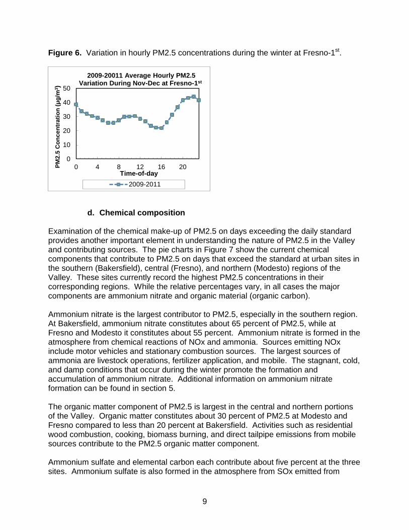
c. Source apportionment using source receptor models Source receptor models (also known as observational models) can be used to determine the relative importance of the different types of PM2.5 emission sources at individual monitoring sites. The Chemical Mass Balance (CMB) model statistically relates measured chemical species of ambient PM2.5 to the chemical species emitted by diverse sources. The Positive Matrix Factorization (PMF) statistical model distinguishes correlation patterns among measured PM2.5 species to identify sources. Previous studies have applied source apportionment models to IMS-95 and CRPAQS data. For the present study, both CMB and PMF were applied to recent PM2.5 data collected in the San Joaquin Valley.

Prior Source Apportionment Studies In earlier studies, Schauer and Cass, 2000 estimated source contributions to wintertime PM2.5 through CMB modeling of data collected during the IMS-95 field study. Chen et al., 2007, applied two types of multivariate statistical models, PMF and UNMIX, to identify sources contributing to wintertime PM2.5 during the CRPAQS field study. In addition, Chow et al., 2005, applied CMB to the CRPAQS data set. Table 3 summarizes the source contributions to wintertime PM2.5 estimated through these studies. In all cases, ammonium nitrate is the major source, contributing approximately 50 percent to wintertime PM2.5 throughout the Valley (23-site average); ranging from 40 and 50 percent at urban sites (Fresno and Bakersfield) to around 65 percent at rural sites (Kern Wildlife Refuge and Angiola). The combined biomass burning and cooking source, dominated by biomass burning, contributes over 25 percent of PM2.5

05

1015202530354045

Perc

ent C

ontr

ibut

ion

Wood Smoke Contribution to PM2.5 at Fresno-1st

38

Table 3. Wintertime PM2.5 source contributions estimates for IMS-95 and CRPAQS.

Source Contribution Estimates (% of PM2.5 mass) Study and

Sites Salt Dust Exhaust Biom Burn Cook Amm.

Sulfate Amm. Nitrate

Sec Orga Misc

Gas Dies IMS-951 Fresno avg. of 12/26-28/1995 and 1/4-6/1996

- 1.0 2.5 9.6 37.8 6.4 4.8 32.6 4.9 0.5

Bakersfield avg. of 12/26-28/1995 and 1/4-6/1996

- 1.5 3.4 9.5 18.6 5.1 7.5 41.6 12.1 0.7

Kern WR avg. of 12/26-28/1995 and 1/4-6/1996

- 0.9 0 5.0 0.5 0.0 7.9 66.8 15.6 3.2

CRPAQS, UNMIX2

23-site avg. Nov. 2000 - Jan. 2001

0 3 15 24 5 51 2

CRPAQS, PMF2

23-site avg. Nov. 2000 - Jan. 2001

0 5 10 23 3 48 11

CRPAQS, CMB3

Fresno IOPs4 0.2 0.3 1.5 5.8 48.9 3.1 40.1

Bakersfield IOPs4 0.2 1.2 6.4 4.5 30.4 3.9 53.5

Angiola IOPs4 0.3 5.2 7.4 1.9 14.8 4.4 65.9

Sierra Nevada Foothills IOPs4

0.2 1.2 4.0 7.4 41.8 4.7 40.6

1 Schauer and Cass, 2000. 2 Chen et al., 2007. 3 Chow et al., 2005. 4 IOPs = Intensive Operating Periods, 12/15-18/200, 12/26-28/2000, 1/4-6/2001, and 1/31/2001- 2/3/2001. a Secondary organic aerosol estimated from organic carbon not accounted for by primary source profiles.

39

valley wide, constituting the second major source at urban sites – with larger contributions at Fresno than at Bakersfield. In contrast, biomass burning and cooking are not a major sources at rural sites. Engine exhaust, dominated by diesel, is the third major source of directly emitted PM2.5, contributing approximately 10 to 15 percent to PM2.5 valley wide. Since secondary organics are estimated from the organic carbon not accounted for by the apportionment of other organic carbon sources, small changes in the organic carbon content in the chemical composition profiles for other sources may impact the estimate of the secondary organics contribution.

Recent Source Apportionment Studies

Chemical Mass Balance Modeling

Source contributions during high PM2.5 concentration days at Bakersfield-California (BAC) and Fresno –1st Street (FSF) were estimated by applying the CMB model version 8.2 to individual PM2.5 samples using PM2.5 source profiles developed during previous studies. The PM2.5 samples were from days measuring concentrations greater than 30 µg/m3 between 2007 and 2010. Per U.S. EPA guidance, between 2007 and 2009, the carbon collection and analysis method was changed to improve comparability with the rural Interagency Monitoring of Protected Visual Environments (IMPROVE) PM2.5 carbon data. Since the new carbon method started operating in May 2007 at Bakersfield and in April 2009 at Fresno, the CMB analysis relied on 2007-2010 data from Bakersfield and 2009-2010 data from Fresno. Appendix 2 describes this CMB analysis in further detail.

Figure 29 shows the calculated contributions to ambient PM2.5 from sources included in the CMB model. Ammonium nitrate, the most significant source, contributed 67 percent at Bakersfield and 54 percent at Fresno-1st. Biomass burning, which included residential wood combustion and agricultural, prescribed burning, and likely also cooking, contributed nine percent at Bakersfield and 23 percent at Fresno. Motor vehicle exhaust (diesel and gasoline combined) accounted for ten percent at Bakersfield and 12 percent at Fresno-1st. Ammonium sulfate contributed eight percent at Bakersfield and six percent at Fresno-1st. Contributions of the remaining sources were minor at both sites.

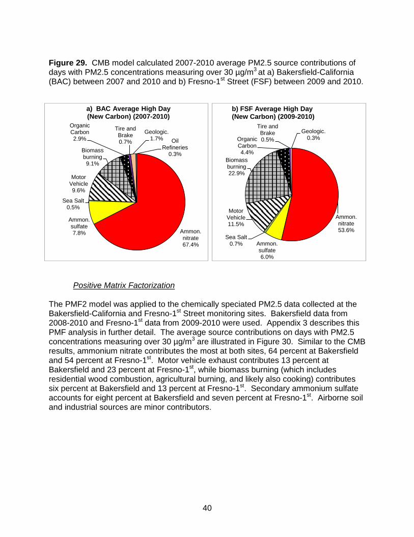
40

Figure 29. CMB model calculated 2007-2010 average PM2.5 source contributions of days with PM2.5 concentrations measuring over 30 µg/m3 at a) Bakersfield-California (BAC) between 2007 and 2010 and b) Fresno-1st Street (FSF) between 2009 and 2010.

Positive Matrix Factorization The PMF2 model was applied to the chemically speciated PM2.5 data collected at the Bakersfield-California and Fresno-1st Street monitoring sites. Bakersfield data from 2008-2010 and Fresno-1st data from 2009-2010 were used. Appendix 3 describes this PMF analysis in further detail. The average source contributions on days with PM2.5 concentrations measuring over 30 µg/m3 are illustrated in Figure 30. Similar to the CMB results, ammonium nitrate contributes the most at both sites, 64 percent at Bakersfield and 54 percent at Fresno-1st. Motor vehicle exhaust contributes 13 percent at Bakersfield and 23 percent at Fresno-1st, while biomass burning (which includes residential wood combustion, agricultural burning, and likely also cooking) contributes six percent at Bakersfield and 13 percent at Fresno-1st. Secondary ammonium sulfate accounts for eight percent at Bakersfield and seven percent at Fresno-1st. Airborne soil and industrial sources are minor contributors.

Ammon. nitrate 53.6%

Ammon. sulfate 6.0%

Sea Salt 0.7%

Motor Vehicle 11.5%

Biomass burning 22.9%

Organic Carbon 4.4%

Tire and Brake 0.5%

Geologic. 0.3%

b) FSF Average High Day (New Carbon) (2009-2010)

Ammon. nitrate 67.4%

Ammon. sulfate 7.8%

Sea Salt 0.5%

Motor Vehicle 9.6%

Biomass burning 9.1%

Organic Carbon 2.9%

Tire and Brake 0.7%

Geologic. 1.7% Oil

Refineries 0.3%

a) BAC Average High Day (New Carbon) (2007-2010)

41

Figure 30. Average high day source contributions estimated using PMF on days with PM2.5 concentrations measuring over 30 µg/m3 at a) Bakersfield-California (BAC) between 2008 and 2010 and b) Fresno-1st Street (FSF) between 2009 and 2010.

While the absolute magnitude of the contributions estimated by the two models vary to some extent, taken together, the CMB and PMF source apportionment studies confirm the importance of secondary ammonium nitrate contributions to PM2.5 on high concentration days. In addition, motor vehicle exhaust and biomass burning were found to be significant contributors to primary PM2.5.

d. Photochemical modeling source apportionment While observational models like CMB and PMF are most useful in identifying sources of primary PM2.5, photochemical models are needed to identify sources of secondary PM2.5. Ying et al. (2008, 2009) simulated the 2000/2001 CRPAQS PM2.5 episode using the source-oriented UCD-CIT air quality model. Source apportionment of primary PM2.5 in the SJV found elemental and organic carbon (EC and OC) to be the two largest components. Wood burning was the major OC source in the Valley, contributing approximately 50 percent to the total PM2.5. At Fresno, wood burning accounted for approximately 70 to 80 percent of the OC, while meat cooking accounted for approximately 10 to 15 percent. Diesel engines were identified as the major EC source. These results are generally consistent with those of the receptor modeling discussed above. Source apportionment of secondary nitrate at Fresno revealed diesel engines were the largest contributor to nitrate, accounting for approximately 40 percent of the PM2.5 nitrate, while catalyst equipped gasoline engines accounted for approximately 20 percent. Agricultural sources accounted for approximately 80 percent of the PM2.5 ammonium.

42

8. PM2.5 AIR QUALITY PROGRESS

a. Annual PM2.5 trends On an annual average basis, PM2.5 air quality has improved over the last ten years. As shown in Figure 31, annual design values at sites in the northern (e.g., Modesto), central (e.g., Fresno-1st) and southern regions (e.g., Bakersfield) in the Valley show progress towards attainment of the standard. The design value -- the metric used to determine compliance with the standard -- represents the average of three consecutive annual averages of the PM2.5 concentrations measured at a specific site (e.g. the 2011 PM2.5 annual design value is the average of the 2009, 2010, and 2011 annual average PM2.5 concentrations). If the annual design value is equal to or below 15.0 μg/m3, the site attains the standard. Between 2001 and 2011, annual design values in the Valley declined between 30 and 40 percent. The largest decreases occurred in the northern and central Valley, where, based on 2011 design values, most sites attain the annual PM2.5 standard. While the southern Valley has shown less improvement, sites are nearing attainment, with design values about 10 to 20 percent over the standard. With on-going implementation of the 2008 PM2.5 Plan, air quality in the Valley is expected to continue to improve and reach attainment in 2014. Figure 31. Trend in annual PM25 design values (2001-2011) at the Bakersfield-California, Fresno-1st, and Modesto monitoring sites.

0

5

10

15

20

25

30

2001 2002 2003 2004 2005 2006 2007 2008 2009 2010 2011

Des

ign

Valu

e (µ

g/m

3 )

Change in Annual PM2.5 Design Values

Bakersfield-California Fresno-1st Modesto

Standard

43

b. 24-Hour PM2.5 trends As illustrated in Figure 32, over the long-term, the 24-hour PM2.5 design values also show a downward trend. The most pronounced progress occurred between 2001 and 2003. Extensive wildfires occurred during the summer of 2008 in Northern California. These wildfires adversely impacted the 2008, 2009, and 2010 design values throughout the Valley, with a greater impact in the northern Valley. Overall, between 2001 and 2011, the 24-hour PM2.5 design values in the Valley have decreased between 30 and 55 percent. Figure 32. Trend in 24-Hour PM2.5 Design Values (2001-2011) at the Bakersfield-California, Fresno-1st, and Modesto monitoring sites.

Meeting the PM2.5 24-hour standard poses a significant challenge because the focus is on the most severe days, which are strongly influenced by meteorology as well as emissions from episodic activities, such as residential wood burning. Thus, evaluating multiple PM2.5 air quality parameters and the meteorology effects on air quality trends provides a broader picture of progress in the Valley. Looking at the number of days with measured PM2.5 concentrations over the 35 µg/m3 standard provides another way to assess PM2.5 trends. Over the long term, between 1999 and 2011, the number of days exceeding the standard decreased by about 50 percent at the Bakersfield-California site and by about 45 percent at the Fresno-1st site (Figure 33). The increase in the number of exceedance days in 2011 compared to 2010 was due to the very severe meteorological conditions experienced in the Valley during the winter of 2011. The Valley experienced similar meteorological conditions during the 1999-2000 and 2000-2001 winters. The total number of exeedance days, however, was much higher during these earlier years, providing evidence that the

0102030405060708090

100

2001 2002 2003 2004 2005 2006 2007 2008 2009 2010 2011

PM2.

5 D

esig

n Va

lue

(µg/

m3 )

Change in 24-Hour PM2.5 Design Values

Bakersfield-CA Fresno-1st ModestoInclude wildfire impacts

44

emission reductions achieved in the Valley have resulted in significant PM2.5 air quality improvement. Figure 33. Trend in measured days over the 24-Hour standard of 35 µg/m3 (1999-2011) at the Bakersfield-California and Fresno-1st monitoring sites.

c. Meteorology impacts on air quality

Although the San Joaquin Valley is large, almost 250 miles long and 80 miles wide, it has a reasonably uniform climatology characterized by hot, dry summers and cool, rainy winters. Mountains on the eastern, western, and southern edges create a long deep basin that can allow pollutants to accumulate under stagnant weather conditions.

The “Pacific High”, a semi-permanent subtropical high pressure system located off the west coast of North America, and the “Great Basin High”, a high pressure region that forms in the winter to the area east of the Sierra Nevada Mountains, are major influences on Valley weather, particularly in the winter. In turn, the strength and position of these high pressure regions are influenced by the strength of the El Nino/Southern Oscillation. El Nino years, characterized by warmer than normal temperatures in the equatorial Pacific and La Nina years, characterized by colder than normal temperatures, can alter the position of the Pacific High, allowing or blocking the passage of frontal systems through California and the San Joaquin Valley. A strong La Nina year can keep the Pacific High from moving south in the winter, diverting normal winter frontal systems northward, and resulting in drier conditions in California, particularly in the southern portions of the State. Due to decreases in the number and strength of frontal systems passing through the Valley, as well as increases in potential stagnant conditions, a strong La Nina year can result in higher than expected PM2.5 concentrations.

0

10

20

30

40

50

60

70

80

1999 2000 2001 2002 2003 2004 2005 2006 2007 2008 2009 2010 2011

Num

ber o

f day

s

Measured Days over 24-Hour PM2.5 Standard of 35 ug/m3

Bakersfield-CA Fresno-1stInclude wildfire impacts

45

In a normal year, when the Pacific High moves south in winter and diminishes in strength, storms can penetrate further into the Valley, bringing clouds and rain. In between these storms, higher pressure can build, bringing mild, bright, sunny weather. A strong Great Basin High can direct winds into the Valley, cleaning out any accumulated particulates. When the Great Basin High is weak, cool, damp air can be trapped in the Valley, with stagnant conditions and poor ventilation lasting for days. The frontal systems which pass through the Valley in winter are weaker than those in the summer and the approach of a weak, slow-moving system can bring light surface winds with weak vertical mixing. The resulting stagnant conditions can persist for extended periods before the frontal system bringing precipitation and stronger winds finally passes through the area. The southern portion of the Valley is effectively blocked by the Tehachapis and the Coast Ranges to the south and west, leaving it dependent on frontal systems from the north for much needed precipitation and winds to scour out any accumulated pollutants. Stagnant conditions can lead to temperature inversions. Under normal conditions, temperature decreases with height, allowing free upward air flow and dispersion of emissions and pollutants. In contrast, a temperature inversion positions a layer of warm air above cooler air impeding upward air flow. Often the inversion layer is lower than the mountains surrounding the Valley providing a “cap” and effectively trapping pollutants. The frequency and intensity of the two high pressure systems and the speed and intensity of the periodic storm systems that clean the air are expected to cause large variations in year-to-year average wintertime PM2.5 concentrations. Measurements conducted during the CRPAQS winter of 2000/2001 indicated that high PM2.5 concentrations usually occur during days dominated by a strong upper-level ridge of high pressure located over Central California (Figure 34 ) (MacDonald et al., 2006). These days are characterized by light winds, low mixing heights, and limited pollutant dispersion. These PM2.5 episodes can last weeks, making addressing the 24-hour PM2.5 standard in the Valley a significant challenge. Figure 34. Frequency of high PM2.5 days in different regions of the San Joaquin Valley corresponding to different synoptic meteorological conditions during the CRPAQS winter of 2000/2001 (Mac Donald et al., 2006).

46

Examples of the impact of La Nina on Valley weather patterns can be seen during the winters of 2011/2012 and 2000/2001, the period during CRPAQS. As noted above, the winter of 2000/2001 was characterized by the persistence of strong surface high pressure that brought light-to-calm winds and stable, stagnant conditions to the Valley. Several fairly strong frontal systems crossed through the region, bringing precipitation, high wind speeds, and strong vertical mixing, allowing accumulated pollutants to disperse. The winter of 2011/2012 was also characterized by a strong surface high-pressure system, but frontal passages were weaker and drier with less vertical mixing, allowing stagnant conditions to continue for longer periods. The graphs in Figures 35 and 36 compare PM2.5 concentrations measured at Bakersfield and Fresno, respectively, between November 1, 2011 and February 29, 2012 to the PM2.5 concentrations measured during the same four months (November through February) in earlier years (1999/2000 and 2000/2001). The 2011/2012 air quality was much better compared to earlier years for all air quality statistics. Peak 24-hour concentrations were over 40 percent lower. The average concentration during the four months period was also 40 percent lower. The number of days over the 24-hour standard of 35 µg/m3 was cut by about 35 percent. Even more significant was the 70 percent decline in the number of days with very high concentrations (over 65 µg/m3).

Figure 35. Comparison of the 2011/2012 PM2.5 episode to the CRPAQS episodes of 1999/2000 and 2000/2001 at Bakersfield-California.

020406080

100120140160180

11/1

11/7

11/1

311

/19

11/2

512

/112

/712

/13

12/1

912

/25

12/3

11/

61/

121/

181/

241/

30 2/5

2/11

2/17

2/23

2/29

PM2.

5 (u

g/m

3 )

Select PM2.5 Episodes at Bakersfield-California

1999-2000

2000-2001

2011-2012

47

Figure 36. Comparison of the 2011/2012 PM2.5 episode to the CRPAQS episodes of 1999/2000 and 2000/2001 at Fresno 1st.

d. Annual trends adjusted for meteorology To understand the effects of emission reductions on ambient PM2.5 concentration trends, the effects of meteorology need to be separated out as fully as possible. The Classification and Regression Trees (CART) method was used for this purpose in the SJV. CART-defined relationships developed for Bakersfield and Fresno accounted for most, but not all, of the effects of meteorology on the annual PM2.5 trends. One aspect that may not have been fully captured was the role of carryover of PM2.5 during extended duration episodes. Further analysis is underway to better address this impact within the CART analysis. Appendix 4 describes the current CART analysis in further detail. The meteorology-adjusted (met-adjusted) trends in the figures below integrate the CART-defined meteorology-effects. For example, in years with meteorology conditions more conducive to PM2.5 formation, the PM2.5 concentrations were adjusted downward. Conversely, the PM2.5 concentrations were adjusted upward in years with meteorology conditions less conducive to PM2.5 formation. Met-adjusted trends are designed to be better indicators than the observed trends for showing the effects of changing emissions. At Bakersfield, the resulting meteorology-adjusted trend between 1999 and 2010 indicates greater decline in PM2.5 concentrations than the unadjusted trend (Figure 37), while at Fresno the two trends are generally similar (Figure 38). Overall, the meteorology-adjusted trends indicate that between 1999 and 2010, the annual average PM2.5 concentrations decreased about 40 to 50 percent at both locations due to emission reductions.

020406080

100120140160180

11/1

11/7

11/1

311

/19

11/2

512

/112

/712

/13

12/1

912

/25

12/3

11/

61/

121/

181/

241/

30 2/5

2/11

2/17

2/23

2/29

PM2.

5 (u

g/m

3 )

Select PM2.5 Episodes at Fresno-1st

1999-2000

2000-2001

2011-2012

48

Figure 37. Observed and met-adjusted PM2.5 trends in Bakersfield.

Figure 38. Observed and met-adjusted PM2.5 trends in Fresno.

e. 24-hour trends adjusted for meteorology Similar to annual average trends, the number of exceedance days that occur each year can be strongly affected by differences in meteorological conditions from year to year. Figure 39 shows observed and met-adjusted trends for PM2.5 exceedance days in the Bakersfield and Fresno areas. The observed values each year may differ from those in

0

10

20

30

1998 1999 2000 2001 2002 2003 2004 2005 2006 2007 2008 2009 2010 2011

PM2.

5(µ

g/m

3 )

Year

Observed and Met-Adjusted PM2.5 Trends in Bakersfield Area

Observed PM2.5 ConcentrationsMet-Adjusted PM2.5Linear (Observed PM2.5 Concentrations)Linear (Met-Adjusted PM2.5)

0

10

20

30

1998 1999 2000 2001 2002 2003 2004 2005 2006 2007 2008 2009 2010 2011

PM2.

5(µ

g/m

3 )

Year

Observed and Met-Adjusted PM2.5 Trends in Fresno Area

Observed PM2.5 ConcentrationsMet-Adjusted PM2.5Linear (Observed PM2.5 Concentrations)Linear (Met-Adjusted PM2.5)

49

Figure 33 for several reasons including a) they are averages of multiple sites in each area, b) more days could be included where missing values could be imputed (missing values were filled in using relationships in existing data), and c) some days with incomplete meteorological data could not be included in the analysis. The met-adjusted trend for Bakersfield shows a stronger decline compared to the observed trend, while in Fresno the observed and met-adjusted trends are similar. The decrease from 1999 through 2010 for the met-adjusted trend is 60 to 65 percent in both areas. Figure 39. Observed and met-adjusted trends for PM2.5 exceedance days in a) the Bakersfield area and b) the Fresno area.

50

f. Trends in 24-hour, seasonal, and hourly PM2.5 Comparing the change in the frequency distribution of 24-hour PM2.5 concentrations over the last decade provides another means of looking at air quality changes over the years. As illustrated in Figure 40, the fraction of days recording PM2.5 over the 24-hour standard of 35 μg/m3 decreased between the three-year periods of 1999-2001 and 2009-2011 at the three monitoring sites shown. At Bakersfield, the frequency decreased from over 15 to less than ten percent, at Fresno from 20 to less than ten percent, and at Modesto from about ten percent to less than five percent. In contrast, during these same periods, the fraction of days recording concentrations at or below the annual standard increased from about 50 up to 70 percent at Bakersfield, from 55 up to 70 percent at Fresno, and from about 65 up to 80 percent at Modesto. Figure 40. Change in PM2.5 concentration frequency distribution between the 1999-2001 and 2009-2011 periods at the a) Bakersfield-California, b) Fresno-1st, and c) Modesto monitoring sites.

01020304050607080

0-15 >15-25 >25-35 >35-50 >50-65 >65-90 > 90

% o

f Sam

ples

Concentration (ug/m3)

a) Decrease in PM2.5 Concentrations at Bakersfield-California

1999-2001 2009-2011

01020304050607080

0-15 >15-25 >25-35 >35-50 >50-65 >65-90 > 90

% o

f Sam

ples

Concentration (µg/m3)

b ) Decrease in PM2.5 Concentrations at Fresno-1st

1999-2001 2009-2011

0102030405060708090

0-15 >15-25 >25-35 >35-50 >50-65 >65-90 > 90

% o

f Sam

ples

Concentration (ug/m3)

c) Decrease in PM2.5 Concentrations at Modesto

1999-2001 2009-2011

51

In the San Joaquin Valley, PM2.5 concentrations over the 24-hour standard occur during the winter season. Figure 41 illustrates the overall downward trend in the three-year averages of 1st and 4th quarter (Q1+Q4) PM2.5 concentrations between the periods of 1999-2002 and 2009-2011. Over the long-term, Q1+Q4 average PM2.5 concentrations decreased by 37 percent at Bakersfield and Modesto and 47 percent at Fresno. Most recently, between the periods of 2004-2006 and 2009-2011, Q1+Q4 average PM2.5 concentrations decreased by eight percent at Bakersfield, 11 percent at Fresno, and ten percent at Modesto. Figure 41. Change in three-year averages of 1st and 4th quarter PM2.5 concentrations at the Bakersfield-California, Fresno-1st, and Modesto monitoring sites.

0

5

10

15

20

25

30

35

40

45

2001 2002 2003 2004 2005 2006 2007 2008 2009 2010 2011

Con

cent

ratio

n (u

g/m

3 )

Change in Three-Year Averages of 1st and 4th Quarter PM2.5 Concentrations

Bakersfield-CA

Fresno-1st

Modesto

52

Focusing on changes in winter (November through February) average PM2.5 concentrations in years when meteorological conditions were most conducive to PM2.5 formation and accumulation provides further insight into PM2.5 air quality progress. These years include 2000, 2002, 2007, and 2011, which as illustrated on Figure 33, also had the highest numbers of days measuring over the 24-hour PM2.5 standard. Figure 42 illustrates the decrease in the winter average PM2.5 concentrations in these four years at the Bakersfield-California, Fresno-1st, and Modesto monitoring sites. Comparing 2000 to 2011, winter average PM2.5 concentrations decreased by about 35 percent in Bakersfield, about 40 percent in Fresno, and about 30 percent in Modesto. Comparing the more recent years of 2007 and 2011, winter average PM2.5 concentrations decreased by about 30 percent in Bakersfield, 20 percent in Fresno, and ten percent in Modesto. Figure 42. Changes in winter-months average (January, February, November, December) PM2.5 concentrations at the Bakersfield-California, Fresno-1st and Modesto monitoring sites among years with most PM2.5 conducive meteorology.

05

101520253035404550

2000 2002 2007 2011

Con

cent

ratio

n (µ

g/m

3)

Changes in Winter Months Average PM2.5 Concentrations

Bakersfield-CA Fresno-1st Modesto

53

Progress in PM2.5 is further corroborated by comparing changes in monthly average PM2.5 concentrations between 1999-2001 and 2009-2011 (Figure 43). The overall PM2.5 seasonal pattern has not changed; however the average monthly concentrations have decreased. The most significant improvements in PM2.5 have been achieved during the winter months.

Figure 43. Changes in PM2.5 monthly concentrations between the 1999-2001 and 2009-2011 three-year periods at the a) Bakersfield-California, b) Fresno-1st, and c) Modesto monitoring sites.

0

10

20

30

40

50

60

1 2 3 4 5 6 7 8 9 10 11 12

Con

cent

ratio

ns (u

g/m

3)

Month

b) Changes in PM2.5 Seasonal Pattern Fresno-1st

1999-2001 2009-2011

0

10

20

30

40

50

60

1 2 3 4 5 6 7 8 9 10 11 12

Con

cent

ratio

ns (u

g/m

3)

Month

a) Changes in PM2.5 Seasonal Pattern Bakersfield-California

1999-2001 2009-2011

0

10

20

30

40

50

1 2 3 4 5 6 7 8 9 10 11 12

Con

cent

ratio

ns (u

g/m

3)

Month

c) Changes in PM2.5 Seasonal Pattern at Modesto

1999-2001 2009-2011

54

Comparing changes in PM2.5 diurnal patterns offers further insights into the progress achieved. Figure 44 illustrates changes in the three-year averages of hourly PM2.5 concentrations recorded during November and December between 2001-2003 and 2009-2011 at a) Bakersfield-California, b) Fresno-1st, and c) Modesto. The overall diurnal patterns have not changed, yet hourly concentrations have decreased throughout the day. Peak daytime concentrations decreased approximately 20 percent, and peak nighttime concentrations approximately 30 percent. Figure 44. Changes in the average November-December PM2.5 hourly concentrations between the 1999-2001 and 2009-2011 three-year periods at the a) Bakersfield-California, b) Fresno-1st, and c) Modesto monitoring sites.

0

10

20

30

40

50

60

70

0 4 8 12 16 20

PM2.

5 C

once

ntra

tion

(ug/

m3 )

Time-of-day

b) Changes in PM2.5 Diurnal Variation (Nov-Dec) at Fresno-1st Street

2001-2003 2009-2011

0

10

20

30

40

50

60

0 4 8 12 16 20PM2.

5 C

once

ntra

tion

(ug/

m3 )

Time-of-day

a) Changes in PM2.5 Diurnal Variation (Nov-Dec) at Bakersfield-CA

2001-2003 2009-2011

0

10

20

30

40

50

60

0 4 8 12 16 20PM2.

5 C

once

ntra

tion

(ug/

m3 )

Time-of-day

Change in PM2.5 Diurnal Variation (Nov-Dec) at Modesto

2001-2003 2009-2011

55

g. Chemical composition trends As previously discussed, PM2.5 concentrations measured at monitoring sites in the SJV have decreased from the 1999-2001 to the 2009-2011 three-year periods. Trends in individual PM2.5 chemical components, as well as emission inventory trends were evaluated to highlight the main chemical components leading to the progress in PM2.5 air quality and to evaluate the response to State and District control programs. Speciation monitors in the SJV collect data on PM2.5 chemical composition. Figures 45, 46, and 47 illustrate the trends in the individual PM2.5 components at Bakersfield, Fresno, and Modesto. Between 2007 and 2009, the carbon collection and analysis method was changed to improve comparability with the rural IMPROVE PM2.5 carbon data. Since the change was implemented mid-year, there are gaps in carbon data for years with a mix of the old and new methods. Ammonium nitrate, ammonium sulfate, and carbon compounds are the major constituents of PM2.5. On an annual average basis, concentrations of these key constituents have all shown significant decreases. Ammonium nitrate concentrations in the Valley declined about 40 percent between 2002 and 2011. During the same time-frame, concentrations of ammonium sulfate and carbon compounds declined about 20 to 30 percent. The most significant declines occurred between 2002 and 2003, and again between 2007 and 2010. Figure 45. Trends in PM2.5 chemical components at Bakersfield.

0

2

4

6

8

10

12

2002200320042005200620072008200920102011

Con

cent

ratio

ns (u

g/m

3)

Trends in PM2.5 Chemical Components at Bakersfield

Ammonium Nitrate

Ammonium Sulfate

Geological

Elements

OM_Old

EC_New

OM_New

56

Figure 46. Trends in PM2.5 chemical components at Fresno-1st.

Figure 47. Trends in PM2.5 chemical components at Modesto.

The 2012 SJV PM2.5 Plan’s Appendix A describes further analyses on PM2.5 air quality trends.

0

2

4

6

8

10

12

14

2002 2003 2004 2005 2006 2007 2008 2009 2010 2011

Con

cent

ratio

ns (u

g/m

3)

Trends in PM2.5 Chemical Components at Fresno-1st

Ammonium NitrateAmmonium SulfateGeologicalElementsEC_OldOM_OldEC_NewOM_New

0

2

4

6

8

10

12

2002 2003 2004 2005 2006 2007 2008 2009 2010 2011

Con

cent

ratio

ns (u

g/m

3)

Trends in PM2.5 Chemical Components at Modesto

Ammonium NitrateAmmonium SulfateGeologicalElementsEC_OldOM_OldEC_NewOM_New

57

h. Emission inventory trends As specified by U.S. EPA’s PM2.5 implementation rule, required PM2.5 plan precursors are directly emitted PM2.5, NOx, and SOx. As discussed in sections 5 and 6, VOCs and ammonia are not significant precursors in terms of reducing PM2.5 concentrations. Figure 48 illustrates wintertime emission trends in the San Joaquin Valley air basin from 2000 through 2011 for the three key precursors.

• NOx emissions have decreased by 219 tons per day (tpd) or 40 percent. Major reductions occurred in emissions from heavy-duty diesel trucks, stationary combustion sources, and other mobile sources (e.g., farm and off-road equipment, trains)

• Direct PM2.5 emissions decreased by 28 tpd or about 30 percent.

Major reductions occurred in emissions from residential wood combustion and entrained dust.

• SOx decreased by 15 tpd or about 60 percent. Major reductions occurred in emissions from stationary fuel combustion sources and industrial processes.

The combined downward trends in PM2.5 components and emissions of PM2.5, NOx, and SOx indicate that the ongoing control program has had substantial benefits in improving air quality in the SJV and that further emission reductions in the future are expected to provide continuing progress towards attaining the 24-hour PM2.5 standard. Figure 48. PM2.5 and PM2.5 precursor winter emission trends in the San Joaquin Valley.

0

100

200

300

400

500

600

Emis

sion

s (t

pd)

Winter Emission Inventory Trends

NOx

PM2.5

SOx

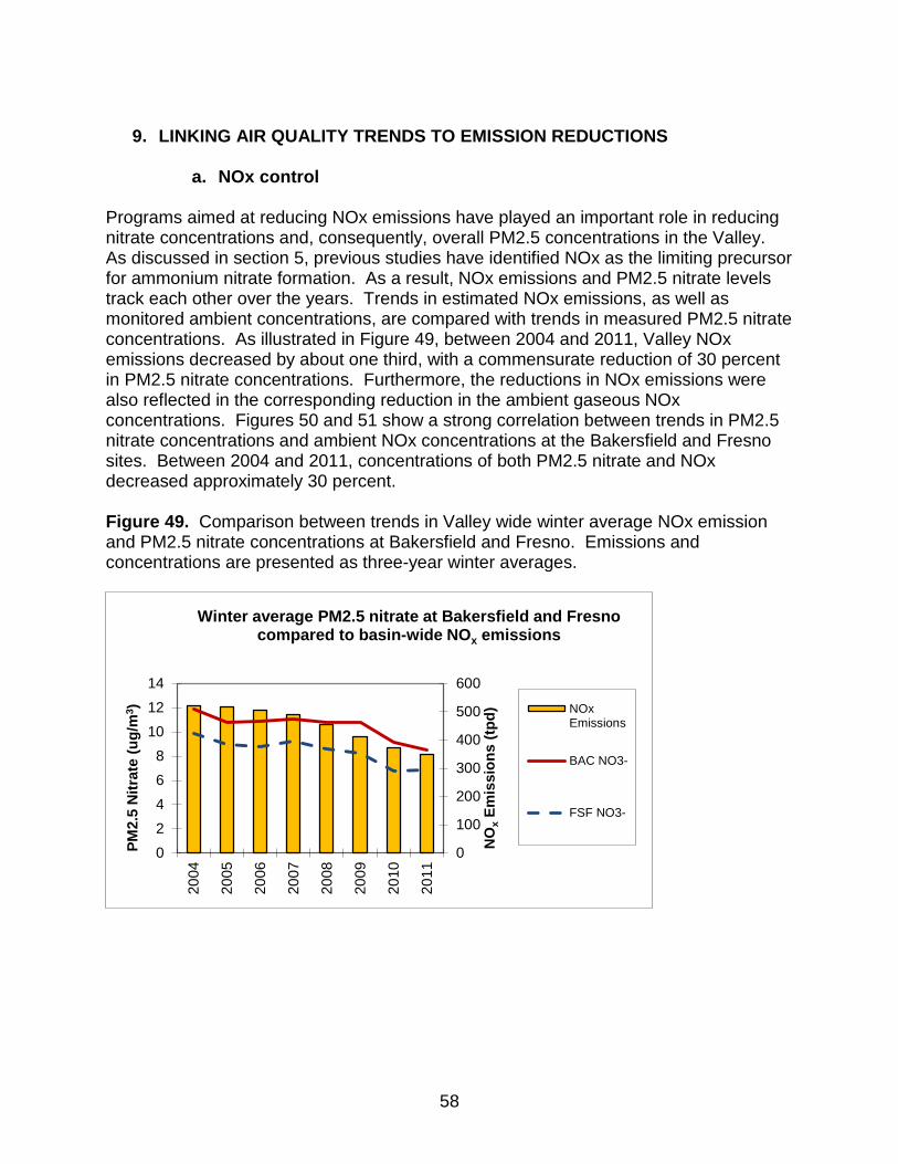
58

9. LINKING AIR QUALITY TRENDS TO EMISSION REDUCTIONS

a. NOx control

Programs aimed at reducing NOx emissions have played an important role in reducing nitrate concentrations and, consequently, overall PM2.5 concentrations in the Valley. As discussed in section 5, previous studies have identified NOx as the limiting precursor for ammonium nitrate formation. As a result, NOx emissions and PM2.5 nitrate levels track each other over the years. Trends in estimated NOx emissions, as well as monitored ambient concentrations, are compared with trends in measured PM2.5 nitrate concentrations. As illustrated in Figure 49, between 2004 and 2011, Valley NOx emissions decreased by about one third, with a commensurate reduction of 30 percent in PM2.5 nitrate concentrations. Furthermore, the reductions in NOx emissions were also reflected in the corresponding reduction in the ambient gaseous NOx concentrations. Figures 50 and 51 show a strong correlation between trends in PM2.5 nitrate concentrations and ambient NOx concentrations at the Bakersfield and Fresno sites. Between 2004 and 2011, concentrations of both PM2.5 nitrate and NOx decreased approximately 30 percent. Figure 49. Comparison between trends in Valley wide winter average NOx emission and PM2.5 nitrate concentrations at Bakersfield and Fresno. Emissions and concentrations are presented as three-year winter averages.

0

100

200

300

400

500

600

02468

101214

2004

2005

2006

2007

2008

2009

2010

2011

NO

x Em

issi

ons

(tpd)

PM2.

5 N

itrat

e (u

g/m

3 )

Winter average PM2.5 nitrate at Bakersfield and Fresno compared to basin-wide NOx emissions

NOxEmissions

BAC NO3-

FSF NO3-

59

Figure 50. Comparison of trends in wintertime PM2.5 nitrate and NOx concentrations in Bakersfield. Concentrations are presented as three-year winter averages.

Figure 51. Comparison of trends in wintertime PM2.5 nitrate and NOx concentrations in Fresno. Concentrations are presented as three-year winter averages.

Because the PM2.5 chemical speciation network is just over ten years old, data from the PM10 ion analysis network were also used to assess longer-term trends. Although, the earlier data do not meet the strict quality assurance/quality control requirements of the PM2.5 chemical speciation network, they do provide a historical perspective. The highest PM10 nitrate concentrations were measured in the Valley in early 90’s. Since then, concentrations of both PM10 nitrate and NOx have decreased about 60 percent (Figure 52). The yearly variability in the ammonium nitrate concentrations reflects the effects of the varying meteorology on ammonium nitrate formation.

0

1

2

3

4

5

6

02468

101214

2004

2005

2006

2007

2008

2009

2010

2011

NO

x (pp

hm)

PM2.

5 N

itrat

e (u

g/m

3 )

Comparison of winter average concentrations of PM2.5 nitrate and NOx in Bakersfield

NOx

NO3-

0

1

2

3

4

5

6

0

2

4

6

8

10

12

2004

2005

2006

2007

2008

2009

2010

2011

NO

x (pp

hm)

PM2.

5 N

itrat

e (u

g/m

3 )

Comparison of winter average concentrations of PM2.5 nitrate and NOx in Fresno

NOx

NO3-

60

Figure 52. Long-term trends in three-year average concentrations of PM10 nitrate and NOx in the San Joaquin Valley.

b. Residential wood burning controls

As previously discussed, annual average concentrations of PM2.5 carbon components have decreased about 20 to 30 percent since 2002. The decrease in the carbon component reflects substantial benefits from the implementation of District Rule 4901, which prohibits residential wood-burning on days when high concentrations of PM2.5 are predicted. In addition, as part of the District’s stringent smoke management program, agricultural burning is prohibited on those same days. Through a series of Rule 4901 amendments, the PM2.5 threshold for calling no-burn days was established in 2003 at 65 μg/m3 and subsequently tightened to 30 μg/m3 in 2008. District staff analyzed the effect that Rule 4901 has had on PM2.5 in the Fresno area using a statistical model developed to quantify PM2.5 reductions attributable to the 2003 and 2008 rule amendments. Based on PM2.5 concentration relationships to meteorological variables before the wood-burning curtailments came into effect, the model predicts what the PM2.5 concentrations would have been if the curtailments had not been adopted. These expected concentrations are then compared to the measured concentrations. This analysis is further described in the 2012 SJV PM2.5 Plan’s Appendix A. The analysis results indicate that as of the 2011-2012 wood-burning season, 24-hour average PM2.5 levels in Fresno have improved by 41 percent (21 μg/m³) since the 2003 and 2008 amendments to Rule 4901 (Figure 53). This improvement is especially marked in PM2.5 concentrations measured during the evening hours of 8:00 p.m. to 12:00 a.m. The average evening PM2.5 concentrations have improved by 50 percent (42 μg/m³) over the same time period. As shown in this analysis, the 2008 amendment

0

1

2

3

4

5

0123456789

10

1987

1988

1989

1990

1991

1992

1993

1994

1995

1996

1997

1998

1999

2000

2001

2002

2003

2004

2005

2006

2007

2008

2009

2010

2011

NO

x (pp

hm)

PM10

Nitr

ate

(ug/

m3 )

Three-year Average Concentrations of PM10 Nitrate and NOx in San Joaquin Valley

NO3-

NOx

61

to Rule 4901 has approximately doubled the seasonal improvements in PM2.5 attributable to the 2003 amendments. Rule 4901 will continue to play an important role in reducing PM2.5 concentrations throughout the San Joaquin Valley both within and beyond the timeframe of this plan. Figure 53: Effect of SJVAPCD’s Rule 4901 on PM2.5 concentrations in Fresno.

62

10. MODELED ATTAINMENT DEMONSTRATION

a. Modeling results Consistent with U.S. EPA guidelines, air quality modeling was done to predict future PM2.5 concentrations at each monitoring site in the San Joaquin Valley. This modeling shows attainment of the 24-hour PM2.5 standard by 2019 in all counties except Kings and Kern, based on implementation of the ongoing control program. In these counties, additional focused emission reductions are needed to provide for attainment. As required by U.S. EPA, additional analyses has been done to confirm that attainment is predicted throughout each county (i.e. in each modeled grid cell). The “Attainment Demonstration” chapter of the District’s plan provides an overview of the photochemical modeling performed. Additional information on the periods modeled, the models selected, and model application can be found in the Modeling Protocol document prepared for this effort. The air quality modeling analysis includes new emission reductions each year between now and 2019 from implementation of a combination of adopted ARB and District programs. As a result, most sites in the northern and central Valley are expected to attain by 2019. As required by U.S. EPA, the modeling replicates the base year 2007 meteorological conditions for each calendar day in the year 2019. The 2007 meteorological conditions included several periods of time especially conducive to the formation of PM2.5. Given the past effectiveness of District programs to curtail residential wood burning, ARB staff then modeled a scenario with an enhanced curtailment program, which would be designed to prevent wood burning on days that may lead up to a PM2.5 exceedance. The modeling results for this scenario indicate that only one site (Bakersfield-California) would not attain the standard with this additional level of control. The predicted design values for each site from this modeling scenario are shown in Table 4. Table 4. 2019 Modeled 24-hour PM2.5 Design Values.

Monitoring Site Design Value (µg/m3) Bakersfield - California 35.7 Bakersfield - Planz 32.9 Corcoran - Patterson 32.1 Visalia - N. Church 29.4 Fresno - Hamilton 28.6 Fresno-1st 30.5 Clovis 28.6 Merced 22.6 Modesto 24.7 Stockton 21.4

63

b. Benefits of emission reductions from on-going programs The implementation of new reductions from California’s on-going emission control programs will provide the major portion of the emission reductions needed to attain the 24-hour PM2.5 standard throughout the San Joaquin Valley in 2019. The PM2.5 design value at the Bakersfield-California site must decrease by approximately 45 percent to demonstrate attainment. Between 2007, the base year used in the photochemical modeling attainment demonstration, and 2019, implementation of these control programs will reduce NOx emissions by 55 percent. Previous sections of this WOE document have demonstrated that prior reductions in NOx have resulted in commensurate reductions in ambient concentrations of nitrate. This is consistent with modeled predictions that demonstrate a nearly 45 percent reduction in ammonium nitrate concentrations. In addition, while directly emitted PM2.5 emissions in aggregate are decreasing by nearly 30 percent, a major focus of the attainment control strategy is further curtailment of residential wood burning. Ambient measurements and modeling studies have shown the large contribution that residential wood burning has on PM2.5 exceedance days. In addition, prior District analysis has demonstrated the significant benefits of past implementation of wood burning curtailment. Therefore, the substantial continuing reductions that will result from implementation of the ongoing control program, coupled with an enhanced residential burning curtailment program, are consistent with the benefits predicted in the modeled attainment demonstration. As a result of the overall control program, coupled with the enhanced wood burning curtailment measure, ammonium nitrate concentrations are predicted to decrease by nearly 45 percent, organic carbon concentrations by approximately 65 percent, and elemental carbon concentrations by nearly 80 percent. A comparison of the concentrations of the main chemical constituents in 2007 to that predicted in 2019 at three sites (Modesto, Fresno-1st, and Bakersfield-California) illustrates the significant reductions in these components (Table 5). Table 5. Comparison of the concentration of chemical constituents for 2007 and 2019 design values at selected sites. Component

(ug/m3) Bakersfield – Calif. Fresno-1st Modesto

2007 2019 2007 2019 2007 2019

Ammonium Nitrate

41.1 22.6 32.1 17.0 28.5 15.6

Ammonium Sulfate

4.7 4.4 3.2 2.5 3.1 2.7

Organic Carbon

15.2 6.6 22.9 8.9 19.7 4.6

Elemental Carbon

2.2 0.5 2.8 0.6 1.6 0.3

64

c. Evaluation of precursor sensitivity

Effectiveness of Valley wide emission reductions In order to determine where to focus the remaining emission reductions needed to bring Bakersfield-California into attainment, as well as identify the attainment plan precursors, ARB staff conducted additional modeling sensitivity runs to assess the relative efficacy of further reductions of different PM2.5 precursors. U.S. EPA’s PM2.5 implementation rule specifies that a precursor is considered “significant” for control strategy development purposes when a significant reduction in the emissions of that precursor pollutant leads to a significant decrease in PM2.5 concentrations. Such pollutants are known as “PM2.5 attainment plan precursors” (72 FR 20586). The U.S. EPA’s implementation rule also establishes a presumption that PM2.5, NOx, and SOx are attainment plan precursors, while VOCs and ammonia are not. In the past for the annual PM2.5 plan, PM2.5, NOx, and SOx were identified and approved as the only attainment plan precursors by U.S. EPA. Results of the annual PM2.5 modeling showed that of these three pollutants, reductions in directly emitted PM2.5 was the most effective. However, because emissions change over time, it is important to continue to assess the attainment plan precursors each time a plan is developed.

Additional photochemical modeling analyses were therefore conducted to understand the relative effectiveness of emission reductions for primary PM2.5 and precursors throughout the Valley in 2019. In these analyses, the model was run with varying combinations of valley wide precursor emission reductions from anthropogenic sources:

• NOx vs. PM2.5 • NOx vs. Ammonia • NOx vs. VOCs • NOx vs. SOx

Table 6 compares the modeled effect on the 2019 design value obtained at each monitoring site from a 25 percent reduction in the specified precursor. Consistently, direct PM2.5 productions have the most benefit, followed by NOx reductions. Reductions in ammonia and SOx provide much smaller benefits, while reductions in VOCs result in very small disbenefits at many sites. Table 7 presents this same information, but normalized to reflect the reduction in design value per ton of each precursor reduced. On this basis, valley wide reductions in PM2.5 are approximately four times as effective as NOx, and approximately five times as effective as SOx. In contrast, reductions in ammonia are approximately nine times less effective than NOx, and as noted above, reductions in VOCs result in either no impact of very small disbenefits.

65

Table 6. Modeled reduction in 2019 PM2.5 design value resulting from 25 percent reduction in valley wide precursor emissions.

Monitoring Site PM2.5 Reduction (µg/m3)

Primary PM2.5

NOx Ammonia SOx VOC

Bakersfield -California 4.44 3.75 0.55 0.18 - 0.10 Bakersfield-Planz 3.80 3.64 0.58 0.19 -0.06 Visalia 3.51 3.10 0.37 0.09 -0.06 Corcoran 3.34 3.99 0.70 0.08 -0.20 Fresno-1st 4.12 2.62 0.51 0.09 0.03 Fresno-Hamilton 3.73 2.57 0.50 0.11 0.05 Clovis 3.29 3.17 0.55 0.09 0.00 Modesto 2.49 1.76 0.43 0.17 0.03 Merced 2.54 2.31 0.34 0.11 -0.01 Stockton 1.87 1.30 0.48 0.20 0.03

Table 7. Modeled PM2.5 air quality benefit per ton of valley wide precursor emission reductions.

Monitoring Site PM2.5 Benefit (µg/m3 per ton reduction)

Primary PM2.5 NOx Ammonia SOx VOC

Bakersfield-California 0.34 0.08 0.008 0.08 -0.001 Bakersfield-Planz 0.29 0.08 0.009 0.08 -0.001 Visalia 0.27 0.07 0.005 0.04 -0.001 Corcoran 0.25 0.09 0.010 0.04 -0.003 Fresno-1st 0.31 0.06 0.008 0.04 0.000 Fresno-Hamilton 0.28 0.06 0.007 0.05 0.001 Clovis 0.25 0.07 0.008 0.04 0.000 Modesto 0.19 0.04 0.006 0.08 0.000 Merced 0.19 0.05 0.005 0.05 0.000 Stockton 0.14 0.03 0.007 0.09 0.000

66

The results of these modeling sensitivity runs were also plotted on isopleth diagrams which reflect the change in the 2019 design value at each level of emission reduction. Isopleth diagrams for the Bakersfield-California site are shown in Figures 54 (a) through (d) to illustrate the overall nature of the modeled response:

• While reducing SOx results in less sulfuric acid and subsequent ammonium sulfate formation, SOx reductions have only a small effect on the predicted design value since ammonium sulfate is a small component of measured PM2.5.

• Reducing VOCs leads to very small increases in the design value because these reductions have the effect of making more NOx available for nitric acid, and subsequent ammonium nitrate formation.

• Because ammonia is much more abundant than NOx, the atmosphere is more responsive to reductions in NOx as compared to ammonia. Reductions in NOx in turn have significant benefits as ammonium nitrate is a large component of measured PM2.5.

• Reductions in directly emitted PM2.5 result in significant benefits due to the reduction in organic carbon which is a large component of measured PM2.5.

These modeling results, along with the findings from past modeling and monitoring studies highlight that reductions in directly emitted PM2.5 and NOx provide the greatest benefit in further reducing PM2.5 concentrations and making progress towards attainment. Given that significant reductions in VOCs and ammonia do not provide significant air quality benefits, per U.S. EPA guidance, the 24-hour PM2.5 attainment plan precursors are directly emitted PM2.5, NOx, and SOx.

67

Figure 54. Bakersfield–California Isopleth Diagrams.

b) NOx vs. VOC

d) NOx vs. PM2.5 c) NOx vs. Ammonia

a) NOx vs. SOx

68

Effectiveness of localized emission reductions

The valley wide precursor sensitivity modeling demonstrates that on a relative basis the greatest benefits are achieved from reductions in sources of directly emitted PM2.5, followed by NOx. Due to the stagnant conditions that occur during wintertime episodes, and the local nature of directly emitted PM2.5 carbon sources in particular, Kern County specific model sensitivity runs were also conducted to evaluate the benefits of emission reductions focused on the nonattainment sub-area. The Kern County sensitivity runs demonstrated that:

• One ton per day of directly emitted PM2.5 reductions provides a 1 µg/m3 improvement in the Bakersfield-California design value;

• One ton per day of NOx reductions provides for a 0.12 µg/m3 improvement in the Bakersfield-California design value;

• One ton per day of SOx reductions provides for a 0.21 µg/m3 improvement in the Bakersfield-California design value;

• One ton per day of ammonia reductions provides for a 0.02 µg/m3 improvement in the Bakersfield-California design value; and

• One ton per day of VOC reductions has no effect on the Bakersfield-California design value.

An examination of sources surrounding the Bakersfield-California monitoring site was then conducted in order to identify potential PM2.5 and NOx sources for further control. The forecasted 2019 PM2.5 and NOx gridded emission inventories were evaluated, focusing on the winter months of November through February when the majority of PM2.5 exceedances occur. The top five emission sources of PM2.5 and NOx in the 9 grid cells (3x3 grid cells, each measuring 4 km x4 km) centered on the Bakersfield-California monitoring site are shown in Figures 55 and 56. The main combustion sources of PM2.5 are commercial cooking, residential fuel combustion, and on-road vehicles. The main NOx source is on-road vehicles, with smaller contributions from off-road equipment, residential fuel combustion, and trains. This analysis suggests that for PM2.5, a focused effort to further reduce residential wood burning and limit emissions from commercial cooking operations would have significant benefits in reducing PM2.5 concentrations in the Bakersfield area. Key NOx sources include on- and off-road mobile sources which are already the focus of ongoing control programs.

69

Figure 55. 2019 top five wintertime PM2.5 emission sources within the Bakersfield-California 9-grid cell area (3x3 grid cells, each measuring 4 km x 4 km with the Bakersfield-California monitor located in the center cell). Wintertime emissions expressed as an average of January, February, November and December emissions.

Figure 56. 2019 top five wintertime NOx emission sources within the Bakersfield-California 9-grid cell area (3x3 grid cells, each measuring 4 km x 4 km with the Bakersfield-California monitor located in the center cell). Wintertime emissions expressed as an average of January, February, November and December emissions.

0.0

0.1

0.2

0.3

0.4

0.5

PM2.

5 Em

issi

ons

(tpd)

2019 top Five Winter PM2.5 Emission Sources withih the Bakersfield-California Nine Grid Cells

0123456

NO

x Em

issi

ons

(tpd)

2019 Top Five Winter NOx Emission Sources within Bakersfield-California Nine Grid Cells

70

d. Demonstrating attainment at Bakersfield-California While adoption of a more stringent wood burning curtailment program brings the Bakersfield-California site very near attainment, further reductions are needed to meet the attainment target of 35.4 µg/m3. Based upon the precursor sensitivity analysis and evaluation of the localized inventory discussed in the previous section, further control of PM2.5 emissions from commercial cooking operations was identified as the most effective approach to provide the emission reductions needed to reach attainment. The final attainment demonstration for the Bakersfield-California design site is provided in Table 8 below:

Table 8. Attainment Demonstration for the Bakersfield-California Design Value Site.

2007 Design Value (µg/m3)

2019 Design Value with Wood

Burning Program Enhancement

(µg/m3)

2019 Final Design Value (µg/m3)

65.6 35.7 ≤35.4 Note: The benchmark for attainment is a design value that is equal to or less than 35.4 µg/m3.

As noted above, the design value in the center column of the table reflects the implementation of ongoing control programs, as well as implementation of an enhanced residential wood burning curtailment program. The final design value reflects the combined impact of further reductions in commercial cooking, as well as a small increase in motor vehicle emissions due to updated vehicle activity data from the San Joaquin Valley Metropolitan Planning Organizations (MPOs). Based on a modeling sensitivity run, implementation of further controls on commercial cooking is expected to result in a 0.6 µg/m3 reduction in the baseline design value. The revised MPO activity data represents approximately one percent of Valley wide NOx emissions. Based on modeling sensitivity runs, this is estimated to result in a design value increase of 0.2 µg/m3. In aggregate, the modeling demonstrates a design value that meets U.S. EPA’s attainment target of 35.4 µg/m3.

71

11. SUMMARY

Consideration of the entirety of information presented in the weight of evidence provides a consistent assessment that supports the modeled attainment date of 2019. The substantial continuing reductions that will result from implementation of the ongoing control program, coupled with new measures addressing residential wood burning and cooking, are consistent with the results predicted in the modeled attainment demonstration. This weight of evidence assessment is based upon the following factors:

• Over the last decade significant progress has occurred in reducing 24-hour PM2.5 concentrations. The 24-hour design value has decreased by over 30 µg/m3, while the number of exceedance days has declined by nearly 50 percent. Meteorologically adjusted trends for the Bakersfield area show an even greater reduction in exceedance days, with a decline of over 60 percent.

• Evaluation of the air quality model response to emission reductions, as well as

model sensitivity runs demonstrates that reductions in directly emitted PM2.5 have the greatest impact per ton of emissions, followed by NOx. For example, in Kern County, PM2.5 emission reductions are approximately eight times more effective than NOx.

• Both receptor and photochemical grid based modeling have identified residential

wood burning as a significant contributor to wintertime PM2.5 concentrations. The reductions in the organic carbon component of PM2.5 that have occurred can be linked to implementation of the District’s residential wood burning curtailment program.

• Evaluation of emissions inventory data, monitoring studies, and photochemical modeling indicate that controlling NOx emissions is the most effective strategy to reduce ammonium nitrate concentrations.

• The decrease in ammonium nitrate concentrations observed at Valley monitoring

sites tracks concurrent reductions in NOx emissions as well as trends in gaseous NOx concentrations.

• Substantial NOx and PM2.5 emission reductions will occur between 2007 and 2019

due to the implementation of on-going measures and additional new measures. As a result of these programs, NOx emissions will decrease by over 50 percent, and PM2.5 emissions by nearly 30 percent.

• The modeled attainment demonstration predicts that all sites in the Valley will attain

by 2019. This modeling assessment is consistent with the benefits seen from previous reductions in the sources and pollutants being addressed as part of the attainment strategy.

72

REFERENCES Blanchard, C.L., Roth, P.M., Tanenbaum, S.J., Ziman, S.D., Seinfeld, J.H., 2000, The use of ambient measurements to identify which precursor species limit aerosol nitrate formation, J. Air & Waste Management Association, 50: 2073-2084. Cai, C. and Kaduwela, A., 2011, Photochemical Air Quality Modeling in California during the CalNex Period,CalNex 2010 Data Analysis Workshop, May 16 – 19, 2011, Joe Serna Jr. Cal/EPA Headquarters Building, 1001 I Street, Sacramento CA (http://www.arb.ca.gov/research/calnex2010/da_workshop_may2011/da_workshop_agenda_w_links.pdf). Chen, J., Ying, Q., and Kleeman, M.J., 2010, Source apportionment of wintertime secondary organic aerosol during the California regional PM10/PM2.5 air quality study, Atmospheric Environment, 44(10), 1331-1340. Chen, L.-W. A., Watson, J.G.; Chow, J.C.; Magliano, K.L., 2007, Quantifying PM2.5 source contributions for the San Joaquin Valley with multivariate receptor models, Environ. Sci. Technol., 41(8): 2818-2826. Chow, J.C.; Chen, L.-W.A.; Lowenthal, D.H.; Doraiswamy, P.; Park, K.; Kohl, S.D.; Trimble, D.L.; Watson, J.G., 2005, California Regional PM10/PM2.5 Air Quality Study (CRPAQS) - Initial data analysis of field program measurements. Report Number 2497; prepared by Desert Research Institute, Reno, NV, for California Air Resources Board, Sacramento, CA. Gorin, C.A.; Collett, J.L., Jr.; Herckes, P., 2005, Wood smoke contribution to winter aerosol in Fresno during winter 2003-2004. prepared by Colorado State Univ, Ft. Collines, CO, http://cospl.coalliance.org/fez/eserv/co:9465/ucsu5810763internet.pdf. Jacob, D.J., Crawford, J.H., Maring, H., Clarke, A.D., Dibb, J.E., Emmons, L.K., Ferrare, R.A., Hostetler, C.A., Russell, P.B., Singh, H.B., Thompson, A.M., Shaw, G.E., McCauley, E., Pederson, J.R., and Fisher, J.A., 2010, The Arctic Research of the Composition of the Troposphere from Aircraft and Satellites (ARCTAS) Mission: Design, Execution, and First Results, Atmospheric Chemistry and Physics, 10(11), 5191-5212. Kaduwela A. and Cai, C., 2009, CARB Simulation of ARCTAS-CA Measurements with MM5/CMAQ Modeling System, Presentation made at the ARCTAS-California Preliminary Data Analysis Workshop, June 30 – July 1, 2009, University of California at Davis, CA (http://www.arb.ca.gov/research/arctas/agenda.htm). Kelly, J.T., Baker, K.R., Cai, C., Avise, J., Jackson, B., and Kaduwela, A., 2011, Preliminary Inter-comparison of Photochemical Modeling by EPA and CARB for the CalNex 2010 Study, Poster presented at the 10th Annual CMAS Conference, Chapel Hill, NC, October 24-26.

73

Kleeman, M.J., Ying, Q., and Kaduwela, A., Control strategies for the reduction of airborne particulate nitrate in California's San Joaquin Valley, Atmospheric Environment, 2005, 39, 5325-5341. Lurmann, F.W., Brown, S.G., McCarthy, M.C., and Roberts, P.T., December 2006, Processes Influencing Secondary Aerosol Formation in the San Joaquin Valley during Winter, Journal of Air and Waste Management Association, 56, 1679-1693. Liang, J., Gürer, K., Allen, P.D., Zhang, K.M., Ying, Q., Kleeman, M., Wexler, A., and Kaduwela, A.,2006, A photochemical model investigation of an extended winter PM episode observed in Central California: Model Performance Evaluation, Proceedings of the 5th Annual CMAQ Models-3 User’s Conference, Chapel Hill, NC. Livingstone, P.L., et. al., 2009, Simulating PM concentrations during a winter episode in a subtropical valley: Sensitivity simulations and evaluation methods, Atmospheric Environment, 43, 5971-5977. MacDonald, C.P.; McCarthy, M.C.; Dye, T.S.; Wheeler, N.J.M.; Hafner, H.R.; Roberts, P.T., 2006, Transport and dispersion during wintertime particulate matter episodes in the San Joaquin Valley, California. J. Air Waste Manage. Assoc., 56(7):961-976. Meng, Z., Dabdub, D., and Seinfeld, J.H., July 1997, Chemical coupling between atmospheric ozone and particulate matter, Science, DOI:10.1126/science.277.5322.116, 116-119. Pun, B.K., and Seigneur, C., 1998, Conceptual model of particulate matter pollution in the California San Joaquin Valley, prepared for Pacific Gas & Electric, Document CP045-1-98. Pun, B.K., and Seigneur, C.,2001, Sensitivity of particulate matter nitrate formation to precursor emissions in the California San Joaquin Valley, Environmental Science and Technology, 35, 2979-2987. Pun, B.K., 2004, CRPAQS Task 2.7 when and where does high O3 correspond to high PM2.5? How much PM2.5 corresponds to photochemical end products? prepared for the San Joaquin Valleywide Air Pollution Study Agency. Pun, B.K., Balmori R.T.F, and Seigneur, C., 2009, Modeling wintertime particulate matter formation in Central California, Atmospheric Environment, 43, 402-409. Schauer, J.J., Cass, G.R., 2000, Source apportionment of wintertime gas-phase and particle-phase air pollutants using organic compounds as tracers, Environ. Sci. Technol. 34(9): 1821-1832.

74

Stockwell, W.R., Watson, J.G., Robinson, N.F., Steiner, W., and Sylte, W.W., 2000, The ammonium nitrate particle equivalent of NOx emissions for wintertime conditions in Central California’s San Joaquin Valley, Atmospheric Environment, 34, 4711-4717. Turkiewicz, K., Magliano, K., Najita, T., 2006, Comparison of two winter air quality episodes during the California Regional Particulate Air Quality Study. J. Air & Waste Manage. Assoc., 56, 467-473. U.S. EPA, 2007, Guidance on the Use of Models and Other Analyses for Demonstrating Attainment of Air Quality Goals for Ozone, PM2.5, and Regional Haze, EPA-454/B07-002. Ying, Q., Lu, J., Kaduwela, A., and Kleeman, M., 2008, Modeling air quality during the California Regional PM10/PM2.5 Air Quality Study (CPRAQS) using the UCD/CIT Source Oriented Air Quality Model - Part II. Regional source apportionment of primary airborne particulate matter, Atmospheric Environment, 42(39), 8967-8978. Ying, Q., Kleeman, M., 2009, Regional contribution to airborne particulate matter in central California during a severe pollution episode. Atmos. Environ., 43, 1218-1228.

Ying, Q., Lu, J., and Kleeman, M., 2009, Modeling air quality during the California Regional PM10/PM2.5 Air Quality Study (CRPAQS) using the UCD/CIT source-oriented air quality model – Part III. Regional source apportionment of secondary and total airborne particulate matter, Atmospheric Environment, 43, 419-430. West, J.J., Ansari, A.S., and Pandis, S.N., 1999, Marginal PM2.5: Nonlinear aerosol mass response to sulfate reductions in the Eastern United States, J. Air & Waste Manage. Assoc., 49, 1415-1424. Watson, J.G.; Chow, J.C., 2002, A wintertime PM2.5 episode at the Fresno, CA, supersite. Atmos. Environ., 36(3):465-475. Watson, J., Roth, P.: Evolving Science in Central California-Why do we need air quality studies? Air Quality Symposium, Fresno, CA, May 17, 2006.

1

San Joaquin Valley PM2.5 Weight of Evidence Analysis

Appendix 1

California Regional PM10/PM2.5 Air Quality Study

Publications

2

CALIFORNIA REGIONAL PM10/PM2.5 AIR QUALITY STUDY

PUBLICATIONS 1. Roth, P. M. et al., 1993, “A Proposed PM-10 Program for the San Joaquin Valley”, prepared by

Envair for the San Joaquin Valleywide Air Pollution Study Agency. 2. Gray, H.A. et al. 1995, “San Joaquin Valley Regional PM10 Study Technical Support Study 5A:

Characterizing Micrometeorological Phenomena: Mixing and Diffusion in Low Wind Speed Stable Conditions”, prepared by Systems Applications International for the San Joaquin Valleywide Air Pollution Study Agency.

3. Gillies, J. et al., 1995, “Literature Review Plan for the San Joaquin Valley Regional Particulate

Study Technical Support Study No. 5: Particle Resuspension”, prepared by the Desert Research Institute for the San Joaquin Valleywide Air Pollution Study Agency.

4. Gillies, J. et al., 1995, “Resuspension of Particles by the Wind: A Literature Review for the San

Joaquin Valley Regional Particulate Study Technical Support Study No. 5: Particle Resuspension”, prepared by the Desert Research Institute for the San Joaquin Valleywide Air Pollution Study Agency.

5. Gillies, J. et al., 1996, “Resuspension of Particles by the Wind: Research Initiatives for California

Regional Particulate Study Technical Support Study No. 5: Particle Resuspension”, prepared by the Desert Research Institute for the San Joaquin Valleywide Air Pollution Study Agency.

6. Gillies, J. et al., 1996, “Resuspension of Particles by the Wind: Modeling, Data Analysis Initiatives

for California Regional Particulate Study Technical Support Study No. 5: Particle Resuspension”, prepared by the Desert Research Institute for the San Joaquin Valleywide Air Pollution Study Agency.

7. Hagan, C. et al., 1996, “California Regional PM10 Air Quality Study: Emissions Modeling Plan”,

prepared by Envair for the San Joaquin Valleywide Air Pollution Study Agency. 8. Roth, P. M. et al., 1996, “Revisions to Cost Estimates for the Central California Fine Particle

Study”, prepared by Envair for the San Joaquin Valleywide Air Pollution Study Agency. 9. Watson, J. et al., 1996, “Data Analysis Activities for the 1995 Integrated Monitoring Study (IMS95)

of the California Regional Particulate Matter Study (CRPAQS)”, prepared by Desert Research Institute for the San Joaquin Valleywide Air Pollution Study Agency.

10. Kumar, N. et al., 1996, “User’s Guide to the UAM-AERO Model”, prepared by Sonoma Technology

Inc. for the San Joaquin Valleywide Air Pollution Study Agency. 11. Kumar, N. et al., 1996, “User’s Guide to the Speciated Rollback Model for Particulate Matter”,

prepared by Sonoma Technology Inc. for the San Joaquin Valleywide Air Pollution Study Agency.

3

12. Lurmann, F. et al., 1996, “PM10 Air Quality Models for Application in the San Joaquin Valley PM10 SIP”, prepared by Sonoma Technology, Inc. for the San Joaquin Valleywide Air Pollution Study Agency.

13. Lehrman, D. E. et al., 1996, “SARMAP II Design: Analysis of the San Joaquin Valley

Meteorological Environment During High PM10 Loading”, prepared by Technical & Business Systems, Inc. for the San Joaquin Valleywide Air Pollution Study Agency.

14. Rogge, W., 1996, “Feasibility of Using Organic Tracers for Tracking the Fate of Primary and

Secondary Aerosols from Combustion Sources”, prepared by Florida International University for the San Joaquin Valleywide Air Pollution Study Agency.

15. Chinkin, L. R. et al., 1996, “Final Workplan for Evaluation and Improvement of Methods for

Determining Ammonia Emissions in the San Joaquin Valley Technical Support Study 5”, prepared by Sonoma Technology, Inc. for the San Joaquin Valleywide Air Pollution Study Agency.

16. Chinkin, L. R., 1996, “CRPAQS TSS15: Task 3, Initial Ammonia Inventory for the San Joaquin

Valley”, prepared by Sonoma Technology, Inc. for the San Joaquin Valleywide Air Pollution Study Agency.

17. Chinkin, L. R. et al., 1996, “Review of Current Methodologies for Estimating Ammonia Emissions”,

prepared by Sonoma Technology, Inc. for the San Joaquin Valleywide Air Pollution Study Agency.

18. Watson, J. G. et al., 1996, “Final Study Plan for: Effectiveness Demonstration of Fugitive Dust

Control Methods for Public Unpaved Roads and Unpaved Shoulders on Paved Roads”, prepared by the Desert Research Institute for the San Joaquin Valleywide Air Pollution Study Agency.

19. Watson, J. G. et al., 1996, “Final Report: Effectiveness Demonstration of Fugitive Dust Control

Methods for Public Unpaved Roads and Unpaved Shoulders on Paved Roads”, prepared by Desert Research Institute for the San Joaquin Valleywide Air Pollution Study Agency.

20. Solomon, P.A. et al., 1996, “1995 Integrated Monitoring Study: Objectives and Design”, presented

at the 1996 U.S. EPA/A&WMA International Symposium on Measurement of Toxic and Related Air Pollutants, Research Triangle Park, NC.

21. Magliano, K.L. et al., 1996, “1995 Integrated Monitoring Study: Temporal Variability of Particulate

Matter - Preliminary Results”, presented at the 1996 U.S. EPA/A&WMA International Symposium on Measurement of Toxic and Related Air Pollutants, Research Triangle Park, NC.

22. Solomon, P.A. et al., 1996, “1995 Integrated Monitoring Study: Spatial and Temporal Variability of

PM10 During the Fall Saturation Study - Preliminary Results”, presented at the 1996 U.S. EPA/A&WMA International Symposium on Measurement of Toxic and Related Air Pollutants, Research Triangle Park, NC.

23. Coe, D. et al., 1996, “Emission Activity Measurement During the Fall andd Winter IMS95

Components - Preliminary Results”, presented at the 1996 U.S. EPA/A&WMA

4

International Symposium on Measurement of Toxic and Related Air Pollutants, Research Triangle Park, NC.

24. Bush, D.H. et al., 1996, “IMS95 Winter Study - Quality Assurance”, presented at the 1996 U.S.

EPA/A&WMA International Symposium on Measurement of Toxic and Related Air Pollutants, Research Triangle Park, NC.

25. Collett, J. et al., 1996, “1995 Integrated Monitoring Study: Fog Measurements in the Southern

Valley - Preliminary Results”, presented at the 1996 U.S. EPA/A&WMA International Symposium on Measurement of Toxic and Related Air Pollutants, Research Triangle Park, NC.

26. Collett, J. et al., 1996, “1995 Integrated Monitoring Study: Fog Measurements in the Northern

Valley - Preliminary Results”, presented at the 1996 U.S. EPA/A&WMA International Symposium on Measurement of Toxic and Related Air Pollutants, Research Triangle Park, NC.

27. Gray, H.A., 1996, “1995 Integrated Monitoring Study: Low Wind Speed Study - Preliminary

Results”, presented at the 1996 U.S. EPA/A&WMA International Symposium on Measurement of Toxic and Related Air Pollutants, Research Triangle Park, NC.

28. Lindsey, C. et al., 1996, “Data Collected by a Network of Radar Profilers, Rawinsonde Sounding

Stations, and Surface Meteorological Monitoring Sites During IMS95”, prepared by Sonoma Technology Inc. for the San Joaquin Valleywide Air Pollution Study Agency.

29. Barnett, A. et al., 1996, “Integrated Measurements Study - 1995 Audit Program Final Report”,

prepared by Aerovironment Environmental Services Inc. for the San Joaquin Valleywide Air Pollution Study Agency.

30. Bush, D. et al., 1996, “IMS95 Winter Study Meteorological Measurements Audits”, prepared by

Aerovironment Environmental Services, Inc. for the San Joaquin Valleywide Air Pollution Study Agency.

31. Ashbaugh, L. A. et al., 1996, “Road Silt Loadings in the San Joaquin Valley During IMS-95”,

prepared by U.C. Davis for the San Joaquin Valleywide Air Pollution Study Agency. 32. Wilson, M., 1996, “Traffic Counts in Support of the 1995 Integrated Monitoring Study”, prepared by

WILTEC for the San Joaquin Valleywide Air Pollution Study Agency. 33. Wilson, M., 1996, “Traffic Counts in Support of the 1995 Integrated Monitoring Study - Axle

Classification Counts”, prepared by WILTEC. 34. Coe, D. et al., 1996, “IMS95 Daily Activity Surveys”, prepared by Sonoma Technology Inc. for the

San Joaquin Valleywide Air Pollution Study Agency. 35. Roberts, P. et al., 1996, “Collection of Continuous Gas-Phase Data at Two Sites During IMS95”,

prepared by Sonoma Technology Inc. for the San Joaquin Valleywide Air Pollution Study Agency.

36. Westerinin, A. et al., 1996, “Final Audit Results for the Integrated Monitoring Study”, prepared by

the Air Resources Board for the San Joaquin Valleywide Air Pollution Study Agency.

5

37. Watson, J. G. et al., 1997, “The Fugitive Dust Characterization Study (FDCS): Potential Methods

and Research Needs for Receptor Methods to Distinguish Among Fugitive Dust Sources”, prepared by Desert Research Institute for the San Joaquin Valleywide Air Pollution Study Agency.

38. Watson, J. G. et al., 1997, “Analysis of Historical PM10 and PM2.5 Measurements in Central

California”, prepared by Desert Research Institute for the San Joaquin Valleywide Air Pollution Study Agency.

39. Ondov, J., 1997, “Technical Support Study No. 13: Feasibility of Using Rare Earth Isotope and

Activatable Tracers for Tracking the Fate of Primary and Secondary Aerosols from Combustion Sources”, prepared by John Ondov for the San Joaquin Valleywide Air Pollution Study Agency.

40. Pankratz, D., 1997, “Quality Assurance Project Plan for Evaluation and Improvement of Methods

for Determining Ammonia Emissions in the San Joaquin Valley”, prepared by Aerovironment for the San Joaquin Valleywide Air Pollution Study Agency.

41. Richards, L. W., 1997, “Technical Support Study 11: Investigating the Dynamics and Chemistry of

Fog Formation and Dissipation - Literature Review”, prepared by Sonoma Technology Inc. for the San Joaquin Valleywide Air Pollution Study Agency.

42. Collett, J. et al., 1997, “Technical Support Study 11: Investigating the Dynamics and Chemistry of

Fog Formation and Dissipation - San Joaquin Valley Fog Measurements During the 1995 Integrated Monitoring Study”, prepared by Colorado State University for the San Joaquin Valleywide Air Pollution Study Agency.

43. Pankratz, D. et al., 1997, “Measurements Report for High Resolution Meteorological Monitoring in

the San Joaquin Valley”, prepared by Aerovironment Environmental Service Inc. for the San Joaquin Valleywide Air Pollution Study Agency.

44. Pandis, S. et al., 1997, “Technical Support Study 11: Investigating the Dynamics and Chemistry of

Fog Formation and Dissipation Paper Copies of References Cited in the Review of Literature on Fogs”, prepared by Carnegie Mellon University for the San Joaquin Valleywide Air Pollution Study Agency.

45. Richards, L. W. et al., 1997, “Technical Support Study 11: Investigating the Dynamics and

Chemistry of Fog Formation and Dissipation Phase II Report Measurement at the Candalabra Tower”, prepared by Sonoma Technology Inc. for the San Joaquin Valleywide Air Pollution Study Agency.

46. Pandis, S. et al., 1997, “Technical Support Study 11: Investigating the Dynamics and Chemistry of

Fog Formation and Dissipation Fog Modeling”, prepared by Carnegie Mellon University for the San Joaquin Valleywide Air Pollution Study Agency.

47. Chow, J. C. et al., 1997, “San Joaquin Valley 1995 Integrated Monitoring Study: Documentation,

Evaluation, and Descriptive Data Analysis of PM10, PM2.5 and Precursor Gas Measurements Technical Support Studies No. 4 and 8”, prepared by the Desert Research Institute for the San Joaquin Valleywide Air Pollution Study Agency.

6

48. Chow, J. C. et al., 1997, “Size-resolved Particle and Light Extinction Measurements During IMS95”, presented at the A&WMAVisual Air Quality - Aerosols and Global Radiation Balance Conference, Bartlett, NH.

49. Solomon, P. A. et al., 1997. “Operational Field Monitoring Plan for the 1995/1996 Integrated

Monitoring Study (IMS95) of the California Regional PM10 Air Quality Study (CRPAQS), Post Field Version, Draft Report”, prepared by Pacific Gas & Electric Company for the San Joaquin Valleywide Air Pollution Study Agency.

50. Solomon, P. A. et al., 1997, “Site Description Report for the 1995 Integrated Monitoring Study

(IMS95) of the California Regional PM10 Air Quality Study (CRPAQS), Post Field Version, Final Report”, prepared by Pacific Gas & Electric Company for the San Joaquin Valleywide Air Pollution Study Agency.

51. Fitz, D., 1997, “Evaluation and Improvement of Methods for Determining Ammonia Emissions in

the San Joaquin Valley Field Data Report”, prepared by University of California, Riverside CE-CERT for the San Joaquin Valleywide Air Pollution Study Agency.

52. McDade, C., 1997, “Ims95 Data Analysis Draft Work Plan for Work Elements 7.3, 7.4, 7.5”,

prepared by ENSR Consulting & Engineering for the San Joaquin Valleywide Air Pollution Study Agency.

53. Magliano, K. L., 1997, “Work Plan for Chemical Mass Balance Modeling of IMS95 Data”, prepared

by the California Air Resources Board for the San Joaquin Valleywide Air Pollution Study Agency.

54. Blanchard, C., 1997, “California Regional PM10 Air Quality Study 1995 Integrated Monitoring

Study Data Analysis Combined Workplan for Tasks 4.2.1 and 4.5.6”, prepared by Envair for the San Joaquin Valleywide Air Pollution Study Agency.

55. Chinkin, L. R. et al., 1997, “IMS 95 Data Analysis Workplans for Tasks 4.1.2, 4.5.1, 4.5.3, 4.6.1,

4.6.2, 4.7.1, and 4.7.2”, prepared by Sonoma Technology, Inc. for the San Joaquin Valleywide Air Pollution Study Agency.

56. Collins, J., 1997, “IMS95 Data Analysis Workplan for Work Element 3.3 Boundaries and

Backgrounds”, prepared by the University of California, Riverside, CE-CERT for the San Joaquin Valleywide Air Pollution Study Agency.

57. Collet, J., 1997, “Work Plan for Work Element 4.6.7”, prepared by Colorado State University for

the San Joaquin Valleywide Air Pollution Study Agency. 58. Collet, J., 1997, “Work Plan for Work Element 4.6.8”, prepared by Colorado State University for

the San Joaquin Valleywide Air Pollution Study Agency. 59. Pandis, S., 1997, “Work Plan for Work Element 4.6.4”, prepared by Carnegie Mellon University for

the San Joaquin Valleywide Air Pollution Study Agency. 60. “Lehrman, D. L., 1997, “Work Plan for IMS95 Analysis Elements 2.2.2 and 2.2.3”, prepared by

Technical & Business Systems, Inc. for the San Joaquin Valleywide Air Pollution Study Agency.

7

61. McDade, C. E., 1997, “Draft Final Report IM95 Data Analysis Work Elements 7.3 Contributions of Chemical Constituents to Visibility Reduction, 7.4 Contributions of Chemical Constituents to Light Extinction Budget, 7.5 Contributions of Emission Sources to Light Extinction Budget”, prepared by ENSR Consulting and Engineering for the San Joaquin Valleywide Air Pollution Study Agency.

62. Chinkin, L. R. et al., 1998, “Use of Ambient Data to Evaluate a Regional Emission Inventory in the

San Joaquin Valley”, presented at the A&WMA PM2.5: A Fine Particle Standard Conference, Long Beach, CA.

63. Coe, D. L. et al., 1998, “Technical Support Study 15: Evaluation and Improvement of Methods for

Determining Ammonia Emissions in the San Joaquin Valley Final Report”, prepared by Sonoma Technology, Inc. for the San Joaquin Valleywide Air Pollution Study Agency.

64. Hackney, R. A. et al., 1998, “Meteorological Data Analysis of Surface, Upper Air, and Synoptic

Conditions during the Integrated Monitoring System 1995 (IMS95) Study Period, from November 1995 through January 1996”, presented at the A&WMA PM2.5: A Fine Particle Standard Conference, Long Beach, CA.

65. Hughes, V. et al., 1998, “Development of the Baseline PM-10 Emissions Inventory for Modeling

and Data Analysis of the IMS-95 Wintertime Field Study”, presented at the A&WMA PM2.5: A Fine Particle Standard Conference, Long Beach, CA.

66. Hoag, K. et al., 1998, “Integrated Monitoring Study 1995: Variations in Fog Chemistry as a

Function of Drop Size and Their Effects on Aerosol Processing”, presented at the A&WMA PM2.5: A Fine Particle Standard Conference, Long Beach, CA.

67. Collett, J. L. et al., 1998, “Integrated Monitoring Study 1995: The Effect of Internal Acid Buffering

on Aerosol Formation in San Joaquin Valley Fogs”, presented at the A&WMA PM2.5: A Fine Particle Standard Conference, Long Beach, CA.

68. Schauer, J. J. et al., 1998, “Source Apportionment of Wintertime Gas-Phase and Particle-Phase

Air Pollutants Using Organic Compounds as Tracers”, presented at the A&WMA PM2.5: A Fine Particle Standard Conference, Long Beach, CA.

69. Kaduwela, A. P. et al., 1998, “Numerical Simulation of Particulate Matter in the San Joaquin

Valley: Application of UAM-AERO to the January 4-6, 1996 Winter Episode”, presented at the A&WMA PM2.5: A Fine Particle Standard Conference, Long Beach, CA.

70. Magliano, K. L. et al., 1998, “Chemical Mass Balance Modeling of the 1995 Integrated Monitoring

Study Database”, presented at the A&WMA PM2.5: A Fine Particle Standard Conference, Long Beach, CA.

71. Coe, D. L. et al., 1998, “The Use of a Day-Specific Source Activity Database to Augment CMB

Source Apportionment Modeling”, presented at the A&WMA PM2.5: A Fine Particle Standard Conference; Long Beach, CA.

72. Kumar, N. et al., 1998, “Evaluation of Gas-Aerosol Phase Distribution of Nitrogen and Sulfur in the

IMS95 Winter Study”, presented at the A&WMA PM2.5: A Fine Particle Standard Conference, Long Beach, CA.

8

73. Richards, L. W. et al., 1998, “1995 Integrated Monitoring Study: Comparison of Light Scattering Measurements During Winter in the San Joaquin Valley”, presented at the A&WMA PM2.5: A Fine Particle Standard Conference, Long Beach, CA.

74. Dye, T. S. et al., 1998, “Mixing Depth Structure and Evolution During the Wintertime in the San

Joaquin Valley as Diagnosed from Upper-Air Meteorological Data”, presented at the A&WMA PM2.5: A Fine Particle Standard Conference, Long Beach, CA.

75. McDade, C. et al., 1998, “Optical Properties of the San Joaquin Valley Aerosol Collected During

the 1995 Integrated Monitoring Study”, presented at the A&WMA PM2.5 : A Fine Particle Standard Conference, Long Beach, CA.

76. Solomon, P.A. et al., 1998, “Overview of the 1995 Integrated Monitoring Study: Field Study, Data

Analysis, and Modeling”, presented at the A&WMA PM2.5: A Fine Particle Standard Conference,; Long Beach, CA.

77. Collett, J. L. et al., 1998, “1995 Integrated Monitoring Study: Measurements at Several Heights on

a TV Tower During Fog Events in the San Joaquin Valley”, presented at the A&WMA PM2.5: A Fine Particle Standard Conference, Long Beach, CA.

78. Blanchard, C. L. et al., 1998, “Spatial and Temporal Variability of Particulate Concentrations and

Composition as Measured in Four Saturation Monitoring Networks During the 1995 Integrated Monitoring Study in the San Joaquin Valley, California”, presented at the A&WMA PM2.5: A Fine Particle Standard Conference, Long Beach, CA.

79. Collett, J. L. et al., 1998, “Final Report: IMS95 Data Analysis Work Element 4.6.8 How Does

Acidification of Drops Due to Aqueous Phase Acid Production Limit Aerosol Formation in Fog Drops”, prepared by Colorado State University for the San Joaquin Valleywide Air Pollution Study Agency.

80. Collett, J. L. et al., 1998, “Final Report: IMS95 Data Analysis Work Element 4.6.7 The Influence of

Drop Size-Dependent Fog Chemistry on Aerosol Production and Deposition in San Joaquin Valley Fogs”, prepared by Colorado State University for the San Joaquin Valleywide Air Pollution Study Agency.

81. Lehrman, D. E. et al., 1998, “Final Report California Regional PM10/PM2.5 Air Quality Study

(CRPAQS) 1995 Integrated Monitoring Study Data Analysis Work Element 2.2.2 - Meteorological Representativeness and Work Element 2.2.3 - Fog And Low Clouds Characteristics”, prepared by Technical & Business Systems, Inc. for the San Joaquin Valleywide Air Pollution Study Agency.

82. Strader, R. et al., 1998, “Final Report 1995 Integrated Monitoring Study Data Analysis 6.5

Evaluation of Secondary Organic Aerosol Formation in Winter”, prepared by Carnegie Mellon University for the San Joaquin Valleywide Air Pollution Study Agency.

83. Pandis, S. et al., 1998, “Final Report 1995 Integrated Monitoring Study Data Analysis Fog Effects

on PM Concentration and Composition in the SJV”, prepared by Carnegie Mellon University for the San Joaquin Valleywide Air Pollution Study Agency.

9

84. Blanchard, C. L. et al., 1998, “Final Report for Tasks 4.2.1 and 4.5.6 Spatial Representativeness of Monitoring Sites and Zones of Influence of Emission Sources”, prepared by Envair for the San Joaquin Valleywide Air Pollution Study Agency.

85. Magliano, K. L. et al., 1998, “Final Report Chemical Mass Balance Modeling of Data from the 1995

Integrated Monitoring Study”, prepared by the California Air Resources Board for the San Joaquin Valleywide Air Pollution Study Agency.

86. Carr, E. L. et al., 1998, “Final Report San Joaquin Valley Regional PM-10 Study Characterizing

Micrometeorological Phenomena: Mixing and Diffusion in Low Wind Speed Conditions Phase III: Monitoring and Data Analysis”, prepared by Systems Applications International for the San Joaquin Valleywide Air Pollution Study Agency.

87. Dye, T. S. et al., 1998, “Measurement Methods Validation: Adequacy and Validation of

Meteorological Measurements Aloft During IMS95”, prepared by Sonoma Technology, Inc. for the San Joaquin Valleywide Air Pollution Study Agency.

88. Coe, D. L. et al., 1998, “Emission Source Activity Detection: Analysis of CMB Model Results and

Daily Activity Data for IMS95”, prepared by Sonoma Technology, Inc. for the San Joaquin Valleywide Air Pollution Study Agency.

89. Main, H. H. et al., 1998, “Characterization of the Spatial and Temporal Patterns of Visibility in the

San Joaquin Valley During IMS95, prepared by Sonoma Technology, Inc. for the San Joaquin Valleywide Air Pollution Study Agency.

90. Carr, E. L. et al., 1998, “1995 Integrated Monitoring Study Data Analysis Work Element 4.6.3:

Time and Length Scales for Mixing of Secondary Aerosols During Stagnation Periods”, prepared by Systems Applications International for the San Joaquin Valleywide Air Pollution Study Agency.

91. Collins, J. F., 1998, “Characterization of Boundaries and Backgrounds in the San Joaquin Valley

Integrated Monitoring Study 1995”, prepared by University of California Riverside CE-CERT for the San Joaquin Valleywide Air Pollution Study Agency.

92. Haste, T. L. et al., 1998, “Use of Ambient Data Collected During IMS95 to Evaluate a Regional

Emissions Inventory for the San Joaquin Valley”, prepared by Sonoma Technology Inc. for the San Joaquin Valleywide Air Pollution Study Agency.

93. Kumar, N., et al., 1998, “Analysis of Atmospheric Chemistry During 1995 Integrated Monitoring

Study”, prepared by Sonoma Technology, Inc. for the San Joaquin Valleywide Air Pollution Study Agency.

94. Magliano, K. L., et al., 1998, “Draft Modeling Protocol for the California Regional PM10/PM2.5 Air

Quality Study: Preliminary Approaches and Data Requirements”, prepared by the California Air Resources Board for the San Joaquin Valleywide Air Pollution Study Agency.

95. Pun, B. et al., 1998, “Comments on Field Program Plan for the California Regional PM10/PM2.5

Air Quality Study”, prepared by Atmospheric and Environmental Research for Pacific Gas & Electric.

10

96. Pun, B. et al., 1998, “Phase II Reports Integrated Monitoring Study 95: Assessment of Mathematical Models and Associated Data Needs”, prepared by Atmospheric and Environmental Research for Pacific Gas & Electric.

97. Pun, B. et al., 1998, “Conceptual Model of Particulate Matter Pollution in the California San

Joaquin Valley”, prepared by Atmospheric and Environmental Research for Pacific Gas & Electric.

98. Richards, W. L. et al., 1998, “Characterization of the Validity of Light Scattering Measurements

During the 1995 Integrated Monitoring Study”, prepared by Sonoma Technology Inc. for the San Joaquin Valleywide Air Pollution Study Agency.

99. Schauer, J. J. et al., 1998, “Source Contributions to Airborne Particles in the San Joaquin Valley

During the IMS95 Study”, prepared by California Institute of Technology for the San Joaquin Valleywide Air Pollution Study Agency.

100. Seinfeld, J. H. et al., 1998, “Grid-Based Aerosol Modeling: A Tutorial”, prepared by California

Institute of Technology for the San Joaquin Valleywide Air Pollution Study Agency. 101. Watson, J. G. et al., 1998, “Aerometric Field Program Plan for the California Regional

PM2.5/PM10 Air Quality Study”, prepared by Desert Research Institute for the San Joaquin Valleywide Air Pollution Study Agency.

102. Wilkinson, J. G., et al., 1998, “A Model to Estimate Temporally Resolved Ammonia Emissions

at a Dairy”, presented at the A&WMA 91st Annual Meeting, San Diego, CA. 103. Richards, W. L. et al., 1999, “Effects of Atmospheric Dynamics and Chemical Concentrations

on Aerosol Formation in Fog ” prepared by Sonoma Technology, Inc. for the San Joaquin Valleywide Air Pollution Study Agency.

104. Magliano, K. L. et al., 1999, “California Regional PM10/PM2.5 Air Quality Study: Objectives

and Associated Data Analysis and Modeling Approaches”, prepared by the California Air Resources Board for the San Joaquin Valleywide Air Pollution Study Agency.

105. Chow, J.C. et al., 1999, “Temporal Variations of PM2.5, PM10, and Gaseous Precursors

During the 1995 Integrated Monitoring Study in Central California”, Atmospheric Environment (33).

106. Collett, J. L. et al., 1999, “Spatial and Temporal Variations in San Joaquin Valley Fog

Chemistry”, Atmospheric Environment (33). 107. Magliano, K. L. et al., 1999, “Recommendations for Emissions Work in Support of the

California Regional PM10/PM2.5 Air Quality Study”, prepared by the California Air Resources Board for the San Joaquin Valleywide Air Pollution Study Agency.

108. Solomon, P. A. et al., 1999, “The 1995 Integrated Monitoring Study (IMS95) of the California

Regional PM10/PM2.5 Air Quality Study (CRPAQS): Study Overview”, Atmospheric Environment (33).

11

109. Solomon, P. A. et al., 1999, “Objectives and Design of Central California’s 1995 Integrated Monitoring Study of the California Regional PM10/PM2.5 Air Quality Study”, Journal A&WMA.

110. Magliano, K. L. et al., 1999, “Spatial and Temporal Variations in PM10 and PM2.5 Source

Contributions and Comparison to Emissions During the 1995 Integrated Monitoring Study”, Atmospheric Environment (33).

111. Lehrman, D. E., et al., 1999, “Assessment of the Methods and Adequacy of Meteorology

Measurements for IMS95”, Atmospheric Environment (33). 112. McDade, C. et al., 1999, “Optical Properties of the San Joaquin Valley Aerosol Collected

During the 1995 Integrated Monitoring Study”, Atmospheric Environment (33). 113. Blanchard, C. L. et al., 1999, “Spatial Scales of Transport and Influence During the 1995

Integrated Monitoring Study in California’s San Joaquin Valley”, Atmospheric Environment (33).

114. Lillis, D. et al., 1999, “Production and Removal of Aerosol in a Polluted Fog Layer - Part I

Model Development and Evaluation”, Atmospheric Environment (33). 115. Lillis, D. et al., 1999, “Production and Removal of Aerosol in a Polluted Fog Layer - Part II

Effects of Fogs on PM in the San Joaquin Valley”, Atmospheric Environment (33). 116. Collett, J. L. et al., 1999, “Internal Acid Buffering in San Joaquin Valley Fog Drops and its

Influence on Aerosol Processing”, Atmospheric Environment (33). 117. Hoag, K, J., et al., 1999, “The Influence of Drop Size-Dependent Fog Chemistry on Aerosol

Processing by San Joaquin Valley Fogs”, Atmospheric Environment (33). 118. Strader, R. et al., 1999, “Evaluation of Secondary Organic Aerosol Formation in Winter”,

Atmospheric Environment (33). 119. Pun, B. et al., 1999, “Understanding Particulate Matter Formation in the California San Joaquin

Valley: Conceptual Model and Data Needs”, Atmospheric Environment (33). 120. Magliano, K. L. et al., 1999, “Field Program Plans for the California Regional PM10/PM2.5 Air

Quality Study”, in Proceedings of the A&WMA 92nd Annual Meeting. 121. Wittig, A. E. et al., 1999, “Health and Safety Plan for the California Regional PM10/PM2.5 Air

Quality Study (CRPAQS)”, prepared by Sonoma Technology Inc. for the San Joaquin Valleywide Air Pollution Study Agency, STI-999215-1894-HASP.

122. Magliano, K.L. et al, 2000, “Coordinated Efforts of the California Regional PM10/PM2.5 Air

Quality Study and the U.S. Environmental Protection Agency Supersite in Fresno, California”, in Proceedings of the 93rd Annual A&WMA Conference, Salt Lake City, UT, June 19-24, 2000.

123. Magliano, K. L. et al., 2000, “Light Scattering Measurements in the California Regional

PM10/PM2.5 Air Quality Study”, In Proceedings of the 93rd Annual A&WMA Conference, Salt Lake City, UT, June 19-24, 2000.

12

124. Schauer, J. J. et al., 2000, “Source Apportionment of Wintertime Gas-Phase and Particle-

Phase Air Pollutants Using Organic Compounds as Tracers”, Environmental Science and Technology (34), 1821-1832.

125. Blanchard, C. L. et al. 2000, “The Use of Ambient Measurements to Identify Which Precursor

Species Limit Aerosol Nitrate Formation”, Journal of the Air and Waste Management Association (50), 2073-2084.

126. Wittig, A. E. et al., 2000, “Quality Integrated Workplan for the Continuous and Filter Air Quality

Measurements in the California Reqional PM10/PM2.5 Air Quality Study (CRPAQS)”, prepared by Sonoma Technology Inc. for the San Joaquin Valleywide Air Pollution Study Agency, STI-999214-1921-QIWP.

127. Flocchini, R. G. et al., 2001, “Sources and Sinks of PM10 in the San Joaquin Valley”, Interim

Report to U.S. Department of Agriculture, Contract Nos. 94-33825-0383 and 98-38825-6063, prepared by University of California Davis.

128. Main, H. et al. 2001, “Managing Data from the California Regional PM10/PM2.5 Air Quality

Study”, in Proceedings of the A&WMA/AGU Regional Haze and Global Radiation Balance Conference, Bend, OR, October 2-5, 2001.

129. Magliano, K.L. et al., 2001, “The California Regional PM10/PM2.5 Air Quality Study

(CRPAQS): Field Study Description and Initial Findings”, in Proceedings of the A&WMA/AGU Regional Haze and Global Radiation Balance Conference, Bend, OR, October 2-5, 2001.

130. Richards, L.W. et al., 2001, “Light Scattering Measurements During the California Regional

PM10/PM2.5 Air Quality Study”, in Proceedings of the A&WMA/AGU Regional Haze and Global Radiation Balance Conference, Bend, OR, October 2-5, 2001.

131. Watson, J. G. et al., 2001, “Comparison of Nephelometer Light Scattering Measurements in

Central California as a Function of Meteorological Variables Particle Size, and Particle Composition”, in Proceedings of the A&WMA/AGU Regional Haze and Global Radiation Balance Conference, Bend, OR, October 2-5, 2001.

132. Chow, J. C. et al., 2001, “Particle Nitrate Measurements at the Fresno Supersite", in

Proceedings of the A&WMA/AGU Regional Haze and Global Radiation Balance Conference, Bend, OR, October 2-5, 2001.

133. Lowenthal, D. H. et al., 2001, “Particle Size Relationships at the Fresno Supersite”, in

Proceedings of the A&WMA/AGU Regional Haze and Global Radiation Balance Conference, Bend, OR, October 2-5, 2001.

134. Pun B. K. et al., 2001; “Sensitivity of Particulate Matter Nitrate Formation to Precursor

Emissions in the California San Joaquin Valley”; Environmental Science and Technology; (35), 2979-2987.

135. Watson, J.G. et al., 2001, “Comparison and Evaluation of In-Situ And Filter Carbon

Measurements at the Fresno Supersite”, Journal of Geophysical Research – Atmospheres”.

13

136. Rappolt, T.J. et al., 2001, “Mapping Air Quality Plumes from Fossil Energy Sources to Assess

the Impacts of Secondary Aerosol Development”, presented at the SPE/EPA/DOE Exploration and Production Environmental Conference, San Antonio, TX, February 2001.

137. Funk, T. et. al., 2001, “Development of Gridded Spatial Allocation Factors for the State of

California”, prepared by Sonoma Technology Inc. for the San Joaquin Valleywide Air Pollution Study Agency.

138. Knuth, W. et al., 2001, “Fall Saturation Network – An Element of the Satellite Network

Operations for the CRPAQS”, prepared by Technical & Business Systems Inc. for the San Joaquin Valleywide Air Pollution Study Agency.

139. Knoderer, C, et. al., 2001, “Data Collected by a 915-MHz Radar Wind Profiler, RASS, and

Surface Meteorological Station at San Martin, California During Fall 2000 and Winter 2001 for the California Regional PM10/PM2.5 Air Quality Study (CRPAQS)”, prepared by Sonoma Technology Inc. for the San Joaquin Valleywide Air Pollution Study Agency.

140. Chung, A. et. al, 2001, “Detection of Alkaline Ultrafine Atmospheric Particles at Bakersfield,

California, Environmental Science Technology, (35), 2184-2190. 141. Bush, D. et al., 2002, “An Evaluation of Portable Nephelometer Performance During

CRPAQS”, presented at A&WMA Symposium on Air Quality Measurement Methods and Technology, November 13-15, 2002.

142. Watson, J. G. et al., 2002, “Air Quality Measurements from the Fresno Supersite”, Journal of

the Air and Waste Management Association, (50), 1321-1334. 143. Watson, J. G. et al., 2002, “A Wintertime PM2.5 Episode at the Fresno, CA, Supersite”,

Atmospheric Environment (36), 465-475. 144. Watson, J.G., 2002, “Particle Size Relationships at the Fresno Supersite”, Journal of the Air

and Waste Management Association, (52), 822-827 145. Herckes, P. et al., 2002, “Organic Matter in Central California Radiation Fogs”, Environmental

Science & Technology, (36), 4777-4782. 146. Hyslop, N. et. al., 2002, “Continuous PM Measurements in a Rural Town in the San Joaquin

Valley”, presented at A&WMA Symposium on Air Quality Measurement Methods and Technology, November 13-15, 2002.

147. Holmen B. A. et al., 2002, “Lidar-Assisted Measurement of PM10 Emissions from Agricultural

Tilling in California’s San Joaquin Valley – Part I: Lidar”, Atmospheric Environment (35), 3251-3264.

148. Holmen B. A. et al., 2002, “Lidar-Assisted Measurement of PM10 Emissions from Agricultural

Tilling in California’s San Joaquin Valley – Part II: Emission Factors”, Atmospheric Environment, (35), 3265-3277.

14

149. Technical & Business Systems Inc., 2002, “Satellite Network Operations for the California Regional PM10/PM2.5 Air Quality Study”, prepared by Technical & Business Systems Inc. for the San Joaquin Valleywide Air Pollution Study Agency.

150. Bush, D. et. al., 2002, “Final Quality Assurance Audit Report California Regional PM10/PM2.5

Air Quality Study”, prepared by Parsons Engineering Science for the San Joaquin Valleywide Air Pollution Study Agency.

151. Stiefer, P. et al., 2002, “Atlas of Ground Truth Surveys”, prepared by Sonoma Technology Inc.

for the San Joaquin Valleywide Air Pollution Study Agency. 152. Engelbrecht, J. P., 2002, “Laboratory Measurement Systems Audit”, prepared by Desert

Research Institute for the San Joaquin Valleywide Air Pollution Study Agency. 153. Countess Environmental, 2002, “Quantifying the Contribution of Fugitive Geological Dust to

Ambient PM10 and PM2.5 Concentrations in the San Joaquin Valley”, prepared for the San Joaquin Valley Air Pollution Control District.

154. Whiteaker, J.R., 2002, “Effects of Meteorological Conditions on Aerosol Composition and

Mixing State in Bakersfield CA”, Environmental Science and Technology, (36), 2345-2353.

155. Ashbaugh, L.L. et al., 2003, “Soil Sample Collection and Analysis for the Fugitive Dust

Characterization Study”, Atmospheric Environment, (37), 1163-1173. 156. Chow, J.C. et al., 2003, “Similarities and Differences in PM10 Chemical Source Profiles for

Geological Dust From the San Joaquin Valley, California”, Atmospheric Environment, (37), 1317-1340.

157. Rinehart, L.R. et al., 2003, “Characterization of PM2.5 Associated Organic Compounds of

Emission Sources Collected During the California Regional PM10/PM2.5 Air Quality Study”, in Proceedings of the 96th Annual A&WMA Conference, San Diego, CA, June 2003.

158. Najita, T. et al., 2003, “Relationship Between PM2.5 and PM10 During the California Reqional

Particulate Air Quality Study”, presented at the 2003 Annual Conference of the American Association for Aerosol Research, Anaheim, CA, October 20-24, 2003.

159. Velasco, P. et al., 2003, “Diurnal Variations in PM2.5, PM10, Chemical Components, Gaseous

Precursors, and Co-Pollutants during the California Regional Particulate Air Quality Study”, presented at the 2003 Annual Conference of the American Association for Aerosol Research, Anaheim, CA, October 20-24, 2003.

160. Turkiewicz, K. et al., 2003, “Spatial and Temporal Variations of PM2.5, PM10, and their

Chemical Components during the California Regional Particulate Air Quality Study”, presented at the 2003 Annual Conference of the American Association for Aerosol Research, Anaheim, CA, October 20-24, 2003.

161. Casuccio, G. et al., 2003, “Characterization of San Joaquin Valley Samples Using Scanning

Electron Microscopy (SEM) Techniques”, presented at the 2003 Annual Conference of the American Association for Aerosol Research, Anaheim, CA, October 20-24, 2003.

15

162. Chow, J. C. et al., 2003, “Spatial and Temporal Variations in PM2.5 Chemical Composition

during Winter, 2000/2001 Episodes in Central California”, presented at the 2003 Annual Conference of the American Association for Aerosol Research, Anaheim, CA, October 20-24, 2003.

163. Watson, J., et al., 2003, “Equivalence and Comparability Among Different PM2.5 Mass

Measurements in Central California”, presented at the 2003 Annual Conference of the American Association for Aerosol Research, Anaheim, CA, October 20-24, 2003.

164. Countess, R. et. al. 2003, “Fugitive Dust Concentrations in the San Joaquin Valley”, presented

at the 2003 Annual Conference of the American Association for Aerosol Research, Anaheim, CA, October 20-24, 2003.

165. Herckes, P. et. al., 2003, “Fog Processing of Atmospheric Organic Compounds During the

California Regional PM10/PM2.5 Air Quality Study (CRPAQS)”, presented at the 2003 Annual Conference of the American Association for Aerosol Research, Anaheim, CA, October 20-24, 2003.

166. McDonald, C. et. al., 2003, “Evaluation of Transport of Particulate Matter and Its Precursors

Into and Out of the San Joaquin Valley, California, Using Two Approaches presented at the 2003 Annual Conference of the American Association for Aerosol Research, Anaheim, CA, October 20-24, 2003.

167. Kleeman, M. et. al., 2003, “Characterization of Atmospheric Nano-Fine Particles at Bakersfield

California”, presented at the 2003 Annual Conference of the American Association for Aerosol Research, Anaheim, CA, October 20-24, 2003.

168. Kleeman, M. et. al., 2003, “Simulating Air Quality in the San Joaquin Valley with a Source-

Oriented Externally Mixed Airshed Model; Evaluation of Model Performance and Control Strategy Effectiveness”, presented at the 2003 Annual Conference of the American Association for Aerosol Research, Anaheim, CA, October 20-24, 2003.

169. Heissler, S. 2003, “Contributions of Chemical Constituents to Visibility Reduction during the

California Regional PM10/PM2.5 Air Quality Study”, presented at the 2003 Annual Conference of the American Association for Aerosol Research, Anaheim, CA, October 20-24, 2003.

170. Countess, R. et. al., 2003, “Contribution of Vegetative Burning to PM2.5 Concentrations in the

San Joaquin Valley”, presented at the 2003 Annual Conference of the American Association for Aerosol Research, Anaheim, CA, October 20-24, 2003.

171. Rappolt, T.J. et. al., 2003, “Near-Term and Low Wind Dispersion Measurements of Plumes

from Steam Generators during the CRPAQS presented at the 2003 Annual Conference of the American Association for Aerosol Research, Anaheim, CA, October 20-24, 2003.

172. Alcorn, S. et. at., 2003, “Comparisons Between California Regional PM10/PM2.5 Air Quality

Study (CRPAQS) Particle Light Scattering and Fine Particle Mass Data”, presented at the 2003 Annual Conference of the American Association for Aerosol Research, Anaheim, CA, October 20-24, 2003.

16

173. Chen, A. et. al., 2003, “Evaluating Similarities of Source Profiles Using Pair Slope Distribution (PSD) Method: Applications to PM2.5 Source Profiles from the BRAVO and CRPAQS Studies”, presented at the 2003 Annual Conference of the American Association for Aerosol Research, Anaheim, CA, October 20-24, 2003.

174. Hyslop, N. et. al., 2003, “Vertical Variations in PM and PM Precursor Concentrations in the

San Joaquin Valley, California”, presented at the 2003 Annual Conference of the American Association for Aerosol Research, Anaheim, CA, October 20-24, 2003.

175. Chang, et. al., 2003, “Aerosol Processing and Removal by Fogs: Observations in Radiation

Fogs During the CRPAQS Study”, presented at the 2003 Annual Conference of the American Association for Aerosol Research, Anaheim, CA, October 20-24, 2003.

176. Chin, et. al., 2003, “Comparison Between Particulate Matter Sampled at Urban and Rural

Locations in the San Joaquin Valley: Continuous Measurement of Single Particle Size and Composition”, presented at the 2003 Annual Conference of the American Association for Aerosol Research, Anaheim, CA, October 20-24, 2003.

177. Rinehart, L. et. al., 2003, “Semi-volatile Organic Compound Characterization and Evaluation of

PM2.5 Emission Sources Collected During the California Regional PM10/PM2.5 Air Quality Study”, presented at the 2003 Annual Conference of the American Association for Aerosol Research, Anaheim, CA, October 20-24, 2003.

178. Hering, S. et. al., 2003, “Temporal and Spatial Distribution of Fine Particle Nitrate and Black

Carbon in the San Joaquin Valley of California, USA”, presented at the 2003 Annual Conference of the American Association for Aerosol Research, Anaheim, CA, October 20-24, 2003.

179. Scow, K. M. et al., 2003, “DNA Profiling Analysis of Dust and Source Material Collected in the

CRPAQS Fall 2000 Sampling Campaign”, prepared by the University of California, Davis for the San Joaquin Valleywide Air Pollution Study Agency.

180. Hafner, H. R., et. al., 2003, “California Reqional PM10/PM2.5 Air Quality Study (CRPAQS)

Management of Anchor Site Data”, prepared by Sonoma Technology Inc for the San Joaquin Valleywide Air Pollution Study Agency, STI-999242-2087-FR.

181. Wittig, A.E., et. al., 2003, “California Regional PM10/PM2.5 Air Quality Study (CRPAQS)

Anchor Site Measurements and Operations”, prepared by Sonoma Technology Inc for the San Joaquin Valleywide Air Pollution Study Agency, STI-999231-2332-FR.

182. Hyslop, N. P., et. al., 2003, “California Regional PM10/PM2.5 Air Quality Study (CRPAQS)

Data Quality Summary Reports”, prepared by Sonoma Technology Inc for the San Joaquin Valleywide Air Pollution Study Agency, STI-999242-2310-FR.

183. Neff, W.D., et. al., 2003, “Final Report Contract 99-4PM A Study of Mesoscale Transport and

Boundary Layer Processes in the Central Valley of California”, prepared by the National Oceanic and Atmospheric Administration for the San Joaquin Valleywide Air Pollution Study Agency.

17

184. Zielinska, B. et. al., 2003, “California Regional PM10/PM2.5 Air Quality Study – Organic Compound Measurements”, prepared by Desert Research Institute for the San Joaquin Valleywide Air Pollution Study Agency.

185. Ervens, B. et. al., 2003, “On the Drop-Size Dependence of Organic Acid and Formaldehyde

Concentrations in Fog”, Journal of Atmospheric Chemistry, (46), 239-269. 186. Whiteaker, J.R., 2003, “Hydroxymethanesulfonate as a Tracer for Fog Processing of Individual

Aerosol Particles”, Atmospheric Environment, (37), 1033-1043. 187. Fitz, D. et. al., 2004, “Development of a Gas and Particulate Matter Organic Speciation Profile

Database”, prepared by the University of California, Riverside Center for Environmental Engineering and Technology for the San Joaquin Valleywide Air Pollution Study Agency.

188. Prather, K., 2004, ATOFMS Field Study Operations Final Report, prepared by the University of

California, San Diego, Prather Research Group for the San Joaquin Valleywide Air Pollution Study Agency.

189. Chow, J.C. et. al., 2004, “Comparison of PM2.5 Chemical Composition from the Fresno

Supersite During Wintertime Pollution Episodes in Central California”, presented at the 13th World Clean Air and Environmental Protection Congress and Exhibition, London England, August 2004.

190. Watson, J.G. et. al., 2004, “Particle Nitrate Sampling Artifacts in California’s San Joaquin

Valley”, presented at the 13th World Clean Air and Environmental Protection Congress and Exhibition, London England, August 2004.

191. DeYoung, R.J. et. al., 2004, “Aerosol Transport in the California Central Valley Observed by

Airborne Lidar” 192. Collett, J.L. et. al., 2004, “The Organic Composition of California Fogs”, submitted to the 3rd

International Conference on Fog and Fog Collection, Capetown, South Africa, October 2004.

193. Carillo, J.H. et. al., 2004, “An Economical Optical Fog Detector”, submitted to the 3rd

International Conference on Fog and Fog Collection, Capetown, South Africa, October 2004.

194. Hyslop, N.P., et. al., 2004, “Exploratory Data Analysis of Particulate Matter Concentrations in

Corcoran, California”, prepared by Sonoma Technology, Inc, for the San Joaquin Valleywide Air Pollution Study Agency, STI-999300-2485-FR.

195. Bahm, K.E. et. al., 2004, “Detecting Source Activities and Reconciling Ambient Measurement

Variations with Field Observations – California Regional PM10 and PM2.5 Air Quality Study (CRPAQS) Data Analysis Task 4.3”, prepared for the San Joaquin Valleywide Air Pollution Study Agency by Sonoma Technology Inc., STI-902328-2579-TM.

196. Baxter, B. et. al., 2004, “Task 1.3 Adequacy and Validity of Meteorological Measurements”,

prepared by Technical & Business Systems for the San Joaquin Valleywide Air Pollution Study Agency.

18

197. Lehrman D. et. al., 2004, “Task 3.3 How Well Do Measurements Characterize Critical

Meteorological Features”, prepared by Technical & Business Systems for the San Joaquin Valleywide Air Pollution Study Agency.

198. Knuth, B., 2004, “Task 5.1 CRPAQS Synoptic Conditions Weather Typing”, prepared by

Technical & Business Systems for the San Joaquin Valleywide Air Pollution Study Agency.

199. Held, T. et. al., 2004, “Modeling Particulate Matter in the San Joaquin Valley with a Source-

Oriented Externally Mixed Three-Dimensional Photochemical Grid Model: Atmospheric Environment, 38(22), 3689-3711.

200. Heisler, S. L., 2004, “Contributions of Chemical Constituents to Visibility Reduction During the

California Regional PM10/PM2.5 Air Quality Study”, prepared by ENSR Corporation for the San Joaquin Valleywide Air Pollution Study Agency.

201. Tracer ES&T, 2004, “California Regional PM10/PM2.5 Air Quality Study (CRPAQS) Initial Data

Analysis of Clean Airship 1 Measurements (Task 6.4)”, prepared by Tracer Environmental Sciences & Technologies, Inc., for the San Joaquin Valleywide Air Pollution Study Agency.

202. Buhr, M.P. et. al., 2004, Examination of Reactive Nitrogen Partitioning at the Bakersfield and

Angiola Field Sites”, prepared by Sonoma Technology Inc. for the San Joaquin Valleywide Air Pollution Study Agency.

203. Buhr, M.P. et. al., 2004, “Comparison and Descriptive Evaluation of the Airborne and Ground-

Based Measurements Collected During the CCOS Field Experiment”, prepared by Sonoma Technology Inc. for the San Joaquin Valleywide Air Pollution Study Agency.

204. Yoho, D. et. al., 2004, “How is Visibility Affected by Atmospheric Constituents, Sources, and

Meteorology – Sources of Light Extinction in the Mojave Desert”, prepared by Technical & Business Systems for the San Joaquin Valleywide Air Pollution Study Agency.

205. Alcorn, S.A. et. al., 2004, “Comparisons Between Light Scattering and Fine-Particle Mass

Data”, prepared by Sonoma Technology Inc. for the San Joaquin Valleywide Air Pollution Study Agency.

206. Pun, B., 2004, “CRPAQS Task 2.7 When and Where Does High O3 Correspond to High

PM2.5? How Much PM2.5 Corresponds to Photochemical End Products?”, prepared by Atmospheric and Environmental Research, Inc. for the San Joaquin Valleywide Air Pollution Study Agency.

207. Collett, J. L. et. al., 2005, “Examination of the Influence of California Regional Particulate Air

Quality Study Fog Episodes on Aerosol Formation and Removal”, prepared by Colorado State University for the San Joaquin Valleywide Air Pollution Study Agency.

208. Raffuse, S. M. et. al., 2005, “Emission Inventory Reconciliation in the San Joaquin Valley”,

prepared by Sonoma Technology Inc. for the San Joaquin Valleywide Air Pollution Study Agency.

19

209. Held, T. et. al., 2005, “A Comparison of the UCD/CIT Air Quality Model and the CMB Source-

Receptor Model for Primary Airborne Particulate Matter”, Atmospheric Environment, (39), 2281-2297.

210. Kleeman, M.J., Ying, Q., Kaduwela, A. 2005. “Control Strategies for the Reduction of Airborne

Particulate Nitrate in California’s San Joaquin Valley”. Atmospheric Environment, (39): 5325-5341.

211. Fahey, K.M., Pandis, S.N., Collett, Jr. J.L., Herckes, P. 2005. “The influence of size-

dependent droplet composition on pollutant processing by fogs”. Atmospheric Environment, (39): 4561-4574.

212. Blanchard, C., 2005, “Comparison of Particulate Nitrate Formation in Different Chemical

Regimes”, presented at the American Association for Aerosol Research (AAAR), Supersites Conference, February 2005, Atlanta, GA.

213. Cahill, T., 2005, “Continuous Analysis of Fresno Aerosols by Size, Time, and Elemental

Concentrations, March – December 2001”, presented at the American Association for Aerosol Research (AAAR), Supersites Conference, February 2005, Atlanta, GA.

214. Collett, J., 2005, “Pollution Processing by Radiation Fogs During the California Regional

PM10/PM2.5 Air Quality Study (CRPAQS)”, presented at the American Association for Aerosol Research (AAAR), Supersites Conference, February 2005, Atlanta, GA.

215. Goohs, K., 2005, “Function and Performance of a New Real-Time Black Carbon Monitor

During the 2004 Fresno Study”, presented at the American Association for Aerosol Research (AAAR), Supersites Conference, February 2005, Atlanta, GA.

216. Herckes, P., 2005, “Fog Processing of Atmospheric Organic Matter”, presented at the

American Association for Aerosol Research (AAAR), Supersites Conference, February 2005, Atlanta, GA.

217. Lurmann, F., 2005, “Spatial Representativeness of the Fresno Supersite PM and Gaseous Co-

Pollutant Measurements”, presented at the American Association for Aerosol Research (AAAR), Supersites Conference, February 2005, Atlanta, GA.

218. Magliano, K., 2005, “Comparison of Air Quality During Two Winter Episodes”, presented at the

American Association for Aerosol Research (AAAR), Supersites Conference, February 2005, Atlanta, GA.

219. Magliano, K., 2005, “PM2.5 Concentrations in Urban and Rural Areas”, presented at the

American Association for Aerosol Research (AAAR), Supersites Conference, February 2005, Atlanta, GA.

220. McCarthy, M., 2005, “The Role of Nighttime Chemistry in Winter Ammonium Nitrate Formation

in the San Joaquin Valley”, presented at the American Association for Aerosol Research (AAAR), Supersites Conference, February 2005, Atlanta, GA.

20

221. Pun, B., 2005, “Relationships Between Ozone and PM During CRPAQS”, presented at the American Association for Aerosol Research (AAAR), Supersites Conference, February 2005, Atlanta, GA.

222. Qin, X., 2005, “ATOFMS Measurements at Urban and Rural Locations: Comparison of Single

Particle Size and Composition”, presented at the American Association for Aerosol Research (AAAR), Supersites Conference, February 2005, Atlanta, GA.

223. Watson, J., 2005, “Spatial Variability of PM2.5 Species in the California Central Valley”,

presented at the American Association for Aerosol Research (AAAR), Supersites Conference, February 2005, Atlanta, GA.

224. Zielinska, B., 2005, “Semi-volatile Organic Compounds: Characterization at the Fresno

Supersite During Wintertime Stagnation Episodes”, presented at the American Association for Aerosol Research (AAAR), Supersites Conference, February 2005, Atlanta, GA.

225. Cassucio, G., 2005, “Corcoran Fall 2000 study: Apportionment of ambient PM10 using

scanning electron microscopy”, presented at the American Association for Aerosol Research (AAAR), Supersites Conference, February 2005, Atlanta, GA.

226. Chow, J., 2005, “Particulate carbon measurements in California's San Joaquin Valley”,

presented at the American Association for Aerosol Research (AAAR), Supersites Conference, February 2005, Atlanta, GA.

227. Chow, J.C., 2005, “Loss of PM2.5 Nitrate from Filter Samples in Central California”, Journal of

the Air and Waste Management Association, (55) 1158-1168. 228. Watson, J.G., et. al., 2005, “Nanoparticle and Ultrafine Particle Events at the Fresno

Supersite”. Journal of the Air & Waste Management Association, (56) 417-430. 229. Gorin, C.A., et. al., 2005, “Wood Smoke Contributions to Ambient Aerosol in Fresno During

Winter 2003-2004”. Prepared for the San Joaquin Valley Air Pollution Control District. Fresno, California.

230. Park, K., et. al., 2005, “Comparison of continuous and filter-based carbon measurements at the Fresno Supersite”. Journal of the Air & Waste Management Association, (56) 474-491.

231. Herner, J.D., et. al., 2005, “Size and Composition Distribution of Airborne Particulate Matter in Northern California 1. Particulate Mass, Carbon, and Water Soluble Ions”, Journal of the Air & Waste Management Association, (55), 30-51.

232. Turkiewicz, K., et. al., 2006, “Comparison of Two Winter Air Quality Episodes During the

California Regional Particulate Air Quality Study”. Journal of the Air & Waste Management Association (56): 467-473.

233. Rinehart, L.R., et. al., 2006, “Spatial Distribution of PM2.5 Associated Organic Compounds in

Central California”. Atmospheric Environment (40): 290-303.

21

234. Chow, J.C., Watson, J.G., Park, K., Lowenthal, D.H., Robinson, N.F., Magliano, K.L., 2006. “Comparison of Particle Light Scattering and PM2.5 Mass in Central California”. Journal of the Air & Waste Management Association (56): 398-410.

235. Chow, J.C., Watson, J.G., Lowenthal, D.H., Chen, A.L-W., Magliano, K.L., 2006. “Particulate

Carbon Measurements in California’s San Joaquin Valley”. Chemosphere (62): 337-348.

236. Chow, J.C., Chen, A.L-W., Watson, J.G., Lowenthal, D.H., Magliano, K.L., Turkiewicz, K.,

Lehrman, D., 2006. “PM2.5 Chemical Composition and Spatiotemporal Variability During the California Regional PM10/PM2.5 Air Quality Study (CRPAQS)”. Journal of Geophysical Research, (111): D10S04, doi:10.1029/2005JD006457.

237. Ying, Q., Kleeman, M.J., 2006. “Source Contributions to the Regional Distribution of Secondary Particulate Matter in California”. Atmospheric Environment (40): 736-752.

238. Herner, J.D., Green, P.G., Kleeman, M.J. 2006. “Measuring the Trace Elemental Composition

of Size-Resolved Airborne Particles”. Environmental Science and Technology (40): 1925-1933.

239. Chow, J.C., Watson, J.G., Lowenthal, D.H., Chen, A.L-W., Tropp, R., Park, K., Magliano, K.L., 2006. “PM2.5 and PM10 Mass Measurements in California’s San Joaquin Valley”. Aerosol Science & Technology (40): 796-810.

240. Lurmann, F. et. al., 2006, “Processes Influencing Secondary Aerosol Formation in the San

Joaquin Valley During Winter”, Journal of the Air & Waste Management Association, (56): 1679-1693.

241. Brown, S.G. et. al., 2006, “Wintertime Vertical Variations in Particulate Matter (PM) and

Precursor Concentrations in the San Joaquin Valley During the California Regional Coarse PM/Fine PM Air Quality Study”, Journal of the Air & Waste Management Association, (56): 1267-1277.

242. MacDonald, C.P. et. al., 2006, “Transport and Dispersion During Wintertime Particulate Matter

Episodes in the San Joaquin Valley, California, Journal of the Air & Waste Management Association, (56): 961-976.

243. Gorin, C.A. et. al., 2006, “Wood Smoke Contribution to Winter Aerosol in Fresno, CA”, Journal

of the Air & Waste Management Association, (56): 1584-1590. 244. Chow, J.C. et. al., 2006, “Evaluation of Organic markers for Chemical Mass Balance Source

Apportionment at the Fresno Supersite”, Atmos. Chem. Phys. Discuss. (6) 10341-10372

245. Grover, B.D. et. al., 2006, “Measurement of Both Volatile and Semi-Volatile Fractions of Fine

Particulate Matter in Fresno, CA”, Aerosol Science & Technology, (40): 811-826. 246. Liang, J. et. al., 2006, “Off-line Diagnostic Analyses of a Three-dimensional PM Model Using

Two Matrix Factorization Methods”, Atmospheric Environment, (40):

22

247. Qin, X. et. al., 2006, “Impact of Biomass Emissions on Particle Chemistry During the California Regional Particulate Air Quality Study”, International Journal of Mass Spectrometry, (258): 142-150.

248. Qin, X. et. al., 2006, “Comparison of Two Methods for Obtaining Quantitative Mass

Concentrations from Aerosol Time-of-Flight Mass Spectrometry Measurements”, Anal. Chem., (78): 6169-6178.

249. Chen, A.L-W., et. al., 2007, “Quantifying PM2.5 Source Contributions for the San Joaquin

Valley with Multivariate Receptor Models”. Environmental Science and Technology, (41), 2818-2826.

250. Hering, et. al., 2007, “Comparison of Particle Size Distributions at Urban and Agricultural Sites

in California’s San Joaquin Valley”. Aerosol Science and Technology, (41:1), 86-96.

251. Watson, J.G. et. al., 2008, “Estimating Aerosol Light Scattering at the Fresno Supersite”, Atmospheric Environment, (42), 1186-1196.

252. Chow, J.C. et.al., 2008, “Size Resolved Aerosol Chemical Concentrations at Rural and Urban

Sites in Central California, USA”, Atmospheric Research, (90), 243-252. 253. Ying, Q. et. al., 2008, “Modeling Air Quality During the California Regional PM10/PM2.5 Air

Quality Study (CRPAQS) Using the UCD/CIT Source Oriented Air Quality Model – Part I. Base Case Model Results”, Atmospheric Environment, (42), 8954-8966.

254. Ying, Q. et. al., 2008, “Modeling Air Quality During the California Regional PM10/PM2.5 Air

Quality Study (CRPAQS) Using the UCD/CIT Source Oriented Air Quality Model – Part II. Regional Source Apportionment of Primary Airborne Particulate Matter”, Atmospheric Environment, (42), 8967-8978.

255. Kleeman, M.J. et.al., 2008, “Size Distribution of Particle-Phase Molecular Markers During a

Severe Winter Pollution Episode”, Environmental Science & Technology, (42), 6469-6475.

256. Ying, Q. et. al., 2008, “Modeling Air Quality During the California Regional PM10/PM2.5 Air

Quality Study (CRPAQS) Using the UCD/CIT Source Oriented Air Quality Model – Part III. Regional Source Apportionment of Secondary and Total Airborne PM2.5 and PM0.1”, Atmospheric Environment, (43), 419-430.

257. Chen, J. et. al., 2009, “Source Apportionment of Visual Impairment During the California

Regional PM10/PM2.5 Air Quality Study, Atmospheric Environment, (43), 6136-6144. 258. Kleeman, M.J., et. al., 2009, “Source Apportionment of Fine (PM1.8) and Ultrafine (PM0.1)

Airborne Particulate Matter During a Severe Winter Pollution Episode, Environmental Science & Technology, (43), 272-279.

259. Livingstone, P.L., et.al., 2009, “Simulating PM Concentrations During a Winter Episode in a

Subtropical Valley and Sensitivity Simulations and Evaluation methods”, Atmospheric Environment, (43), 5971-5977.

23

260. Ying, Q., et. al., 2009, “Regional Contributions to Airborne Particulate Matter in Central California During a Severe Pollution Episode”, Atmospheric Environment, (43), 1218-1228.

261. Pun, B., et. al., 2009, “Modeling Wintertime Particulate Matter Formation in Central California”,

Atmospheric Environment, (43) 402-409. 262. Chen, J., et. al., 2010, “Source Apportionment of Wintertime Secondary Organic Aerosol

During the California Regional PM10/PM2.5 Air Quality Study”, Atmospheric Environment, (44), 1331-1340.

263. Hu, J., et. al., 2010, “Particulate Air Quality Model Predictions Using Prognostic Versus

Diagnostic Meteorology in Central California”, Atmospheric Environment, (44), 215-226.

1

San Joaquin Valley PM2.5 Weight of Evidence Analysis

Appendix 2

PM2.5 Source Apportionment for the San Joaquin Valley Air Basin Using the Chemical Mass Balance Receptor Model

2

PM2.5 Source Apportionment for the San Joaquin Valley Air Basin Using the Chemical Mass Balance Receptor Model

1) Data Collection and Screening

PM2.5 chemical composition data collected at the Bakersfield-California and Fresno-1st Street sites were used for the Chemical Mass Balance (CMB) analysis. The two sites are part of the Chemical Speciation Network (CSN) and use the SASS (Spiral Aerosol Speciation Sampler, Met One, Grants Pass, OR.) for data collection. The Bakersfield-California and Fresno-1st samplers are configured with several channels, each channel containing one 47mmfilter with a 6.7 L/min flow rate. One channel contains a Whatman Teflon®-membrane filter for mass by gravimetry and elements by XRF. Another channel includes a magnesium oxide-coated aluminum (Al) honeycomb after the cyclone followed by a Nylasorb nylon-membrane filter for water-soluble anions i.e., NO3

− and SO4=) and cations (i.e., ammonium [NH4

+] and water-soluble sodium [Na+] and potassium [K+]) by IC. In the past, another channel containing a Whatman QMA quartz-fiber filter was used for OC and EC analysis by the STN thermal/optical transmittance (TOT) protocol. In recent years changes were made to the carbon sampling and analysis method. The collection method changed from the MetOne SASS to the URG3000N sampler, which is very similar to the IMPROVE module C sampler. The analytical method was changed from the NIOSH-like thermal optical transmittance (TOT) method to IMPROVE_A thermal optical reflectance (TOR). A new backup quartz filter is also collected using the URG3000N to help assess artifacts. The backup filter is placed behind the routine quartz sampler filter. This change took place on May 3, 2007 at Bakersfield and April 1, 2009 at Fresno.

Due to the change in carbon collection and analysis method, several data sets were generated for CMB modeling to allow separate analysis of old and new carbon data. Throughout this document we will refer to ‘old carbon’ data and ‘new carbon’ data. Old carbon data were collected using the SASS sampler and analyzed using the NIOSH-like thermal optical transmittance (TOT) method. New carbon data were collected using the modified IMPROVE version II Module C sampler, the URG3000N, and analyzed using the IMPROVE-A thermal optical reflectance (TOR) method. Both old and new carbon data were corrected for sampling artifacts prior to running CMB.

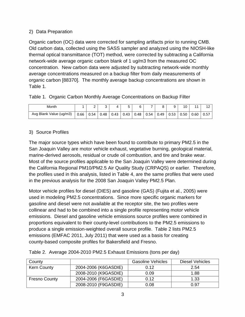
3

2) Data Preparation

Organic carbon (OC) data were corrected for sampling artifacts prior to running CMB. Old carbon data, collected using the SASS sampler and analyzed using the NIOSH-like thermal optical transmittance (TOT) method, were corrected by subtracting a California network-wide average organic carbon blank of 1 ug/m3 from the measured OC concentration. New carbon data were adjusted by subtracting network-wide monthly average concentrations measured on a backup filter from daily measurements of organic carbon [88370]. The monthly average backup concentrations are shown in Table 1.

Table 1. Organic Carbon Monthly Average Concentrations on Backup Filter

Month 1 2 3 4 5 6 7 8 9 10 11 12

Avg Blank Value (ug/m3) 0.66 0.54 0.48 0.43 0.43 0.48 0.54 0.49 0.53 0.50 0.60 0.57

3) Source Profiles

The major source types which have been found to contribute to primary PM2.5 in the San Joaquin Valley are motor vehicle exhaust, vegetative burning, geological material, marine-derived aerosols, residual or crude oil combustion, and tire and brake wear. Most of the source profiles applicable to the San Joaquin Valley were determined during the California Regional PM10/PM2.5 Air Quality Study (CRPAQS) or earlier. Therefore, the profiles used in this analysis, listed in Table 4, are the same profiles that were used in the previous analysis for the 2008 San Joaquin Valley PM2.5 Plan.

Motor vehicle profiles for diesel (DIES) and gasoline (GAS) (Fujita et al., 2005) were used in modeling PM2.5 concentrations. Since more specific organic markers for gasoline and diesel were not available at the receptor site, the two profiles were collinear and had to be combined into a single profile representing motor vehicle emissions. Diesel and gasoline vehicle emissions source profiles were combined in proportions equivalent to their county-level contributions to the PM2.5 emissions to produce a single emission-weighted overall source profile. Table 2 lists PM2.5 emissions (EMFAC 2011, July 2011) that were used as a basis for creating county-based composite profiles for Bakersfield and Fresno.

Table 2. Average 2004-2010 PM2.5 Exhaust Emissions (tons per day)

County Gasoline Vehicles Diesel Vehicles Kern County 2004-2006 (K6GASDIE) 0.12 2.54

2008-2010 (K9GASDIE) 0.09 1.88 Fresno County 2004-2006 (F6GASDIE) 0.12 1.33

2008-2010 (F9GASDIE) 0.08 0.97

4

Table 4. Source Profiles (as Percent of the PM2.5 Mass) Used in the CMB Modeling

PNO 38 35 13 18 41 54 32

SOURCE AMNIT AMSUL WBOakEuc AgBWheat OC MARINE75 TireBrke

N3IC 77.50 ± 7.75 0.00 ± 0.00 0.57 ± 0.07 0.16 ± 0.02 0.00 ± 0.00 22.88 ± 2.60 0.19 ± 1.14

S4IC 0.00 ± 0.00 72.70 ± 7.27 1.30 ± 0.83 0.44 ± 0.04 0.00 ± 0.00 7.20 ± 0.82 0.78 ± 2.10

N4CC 22.55 ± 2.26 27.30 ± 2.73 0.58 ± 0.47 0.59 ± 0.04 0.00 ± 0.00 0.00 ± 0.10 0.16 ± 0.73

NAAC 0.00 ± 0.00 0.00 ± 0.00 0.38 ± 0.15 0.54 ± 0.04 0.00 ± 0.00 28.80 ± 3.27 0.10 ± 0.42

KPAC 0.00 ± 0.00 0.00 ± 0.00 2.89 ± 0.45 6.79 ± 0.50 0.00 ± 0.00 1.07 ± 0.12 0.05 ± 0.17

OCTC 0.00 ± 0.00 0.00 ± 0.00 59.58 ± 4.75 57.03 ± 4.54 100.00 ± 10.00 0.00 ± 0.10 18.81 ± 24.53

ECTC 0.00 ± 0.00 0.00 ± 0.00 5.20 ± 1.12 10.31 ± 0.85 0.00 ± 0.00 0.00 ± 0.10 4.55 ± 5.99

ALXC 0.00 ± 0.00 0.00 ± 0.00 0.07 ± 0.05 0.07 ± 0.01 0.00 ± 0.00 0.00 ± 0.00 0.32 ± 1.89

SIXC 0.00 ± 0.00 0.00 ± 0.00 0.22 ± 0.10 0.13 ± 0.01 0.00 ± 0.00 0.01 ± 0.00 0.69 ± 1.81

PHXC 0.00 ± 0.00 0.00 ± 0.00 0.00 ± 0.01 0.00 ± 0.01 0.00 ± 0.00 0.00 ± 0.00 0.00 ± 0.05

CLXC 0.00 ± 0.00 0.00 ± 0.00 1.72 ± 2.02 6.16 ± 0.44 0.00 ± 0.00 38.74 ± 4.40 0.04 ± 0.08

KPXC 0.00 ± 0.00 0.00 ± 0.00 2.86 ± 0.93 5.50 ± 0.39 0.00 ± 0.00 1.07 ± 0.12 0.10 ± 0.36

CAXC 0.00 ± 0.00 0.00 ± 0.00 0.15 ± 0.10 0.10 ± 0.03 0.00 ± 0.00 1.10 ± 0.12 0.28 ± 1.04

TIXC 0.00 ± 0.00 0.00 ± 0.00 0.01 ± 0.02 0.01 ± 0.01 0.00 ± 0.00 0.00 ± 0.00 0.03 ± 0.38

MNXC 0.00 ± 0.00 0.00 ± 0.00 0.01 ± 0.00 0.00 ± 0.00 0.00 ± 0.00 0.00 ± 0.00 0.48 ± 0.29

FEXC 0.00 ± 0.00 0.00 ± 0.00 0.09 ± 0.06 0.07 ± 0.00 0.00 ± 0.00 0.00 ± 0.00 58.11 ± 31.26

CUXC 0.00 ± 0.00 0.00 ± 0.00 0.01 ± 0.00 1.02 ± 0.07 0.00 ± 0.00 0.00 ± 0.00 0.16 ± 0.69

ZNXC 0.00 ± 0.00 0.00 ± 0.00 0.04 ± 0.02 0.01 ± 0.00 0.00 ± 0.00 0.00 ± 0.00 0.35 ± 2.37

BRXC 0.00 ± 0.00 0.00 ± 0.00 0.00 ± 0.00 0.03 ± 0.00 0.00 ± 0.00 0.18 ± 0.02 0.00 ± 0.01

RBXC 0.00 ± 0.00 0.00 ± 0.00 0.01 ± 0.00 0.00 ± 0.00 0.00 ± 0.00 0.00 ± 0.00 0.01 ± 0.01

SRXC 0.00 ± 0.00 0.00 ± 0.00 0.00 ± 0.00 0.00 ± 0.00 0.00 ± 0.00 0.02 ± 0.00 0.23 ± 0.66

PBXC 0.00 ± 0.00 0.00 ± 0.00 0.00 ± 0.00 0.00 ± 0.00 0.00 ± 0.00 0.00 ± 0.00 0.06 ± 0.03

VAXC 0.00 ± 0.00 0.00 ± 0.00 0.00 ± 0.00 0.00 ± 0.00 0.00 ± 0.00 0.00 ± 0.00 0.00 ± 0.00

NIXC 0.00 ± 0.00 0.00 ± 0.00 0.00 ± 0.00 0.00 ± 0.00 0.00 ± 0.00 0.00 ± 0.00 0.00 ± 0.00

5

Table 4, continued.

PNO 79 80 83 84 66 67 85 86

SOURCE F6GASDIE K6GASDIE F9GASDIE K9GASDIE FDFREANN FDKERANN CHCRUC SFCRUC

N3IC 0.22 ± 1.24 0.16 ± 1.24 0.21 ± 1.24 0.16 ± 1.24 0.02 ± 0.28 0.05 ± 0.16 0.00 ± 0.05 0.00 ± 0.01

S4IC 2.77 ± 7.25 2.60 ± 7.25 2.74 ± 7.25 2.61 ± 7.25 0.56 ± 0.72 0.47 ± 0.29 14.72 ± 6.24 20.32 ± 4.24

N4CC 0.98 ± 3.24 0.89 ± 3.24 0.96 ± 3.24 0.89 ± 3.24 0.04 ± 0.18 0.13 ± 0.20 0.76 ± 0.08 0.01 ± 0.01

NAAC 0.00 ± 0.00 0.00 ± 0.00 0.00 ± 0.00 0.00 ± 0.00 0.17 ± 0.07 0.26 ± 0.24 0.25 ± 0.06 0.76 ± 0.40

KPAC 0.10 ± 0.08 0.10 ± 0.08 0.10 ± 0.08 0.10 ± 0.08 0.27 ± 0.12 0.80 ± 1.25 0.01 ± 0.01 0.06 ± 0.01

OCTC 43.05 ± 27.33 42.40 ± 27.33 42.93 ± 27.33 42.41 ± 27.33 14.34 ± 8.66 10.29 ± 5.32 1.99 ± 1.33 0.09 ± 0.12

ECTC 50.59 ± 17.73 51.50 ± 17.73 50.75 ± 17.73 51.49 ± 17.73 1.92 ± 1.29 0.69 ± 0.72 3.01 ± 1.12 0.00 ± 0.07

ALXC 0.11 ± 0.14 0.11 ± 0.14 0.11 ± 0.14 0.11 ± 0.14 9.97 ± 2.95 7.67 ± 2.53 0.00 ± 0.05 0.00 ± 0.01

SIXC 1.14 ± 4.12 0.99 ± 4.12 1.11 ± 4.12 0.99 ± 4.12 26.77 ± 9.63 22.05 ± 5.29 0.00 ± 0.08 0.01 ± 0.02

PHXC 0.14 ± 0.51 0.13 ± 0.51 0.14 ± 0.51 0.13 ± 0.51 0.33 ± 0.91 0.33 ± 0.91 0.00 ± 0.57 0.00 ± 0.17

CLXC 0.07 ± 0.30 0.06 ± 0.30 0.07 ± 0.30 0.06 ± 0.30 0.11 ± 0.08 0.46 ± 0.48 0.05 ± 0.01 0.02 ± 0.00

KPXC 0.07 ± 0.08 0.07 ± 0.08 0.07 ± 0.08 0.07 ± 0.08 2.30 ± 0.92 3.26 ± 1.59 0.00 ± 0.00 0.04 ± 0.01

CAXC 0.50 ± 1.42 0.49 ± 1.42 0.50 ± 1.42 0.49 ± 1.42 3.01 ± 0.67 5.54 ± 3.03 0.00 ± 0.03 0.06 ± 0.00

TIXC 0.01 ± 0.08 0.01 ± 0.08 0.01 ± 0.08 0.01 ± 0.08 0.48 ± 0.05 0.44 ± 0.24 0.01 ± 0.00 0.01 ± 0.00

MNXC 0.00 ± 0.01 0.00 ± 0.01 0.00 ± 0.01 0.00 ± 0.01 0.11 ± 0.02 0.11 ± 0.08 0.00 ± 0.00 0.01 ± 0.00

FEXC 0.44 ± 0.44 0.44 ± 0.44 0.44 ± 0.44 0.44 ± 0.44 5.30 ± 0.58 5.09 ± 2.84 0.71 ± 0.09 0.21 ± 0.02

CUXC 0.01 ± 0.05 0.01 ± 0.05 0.01 ± 0.05 0.01 ± 0.05 0.02 ± 0.00 0.01 ± 0.01 0.01 ± 0.01 0.00 ± 0.00

ZNXC 0.27 ± 0.41 0.26 ± 0.41 0.27 ± 0.41 0.26 ± 0.41 0.14 ± 0.08 0.07 ± 0.05 0.01 ± 0.00 0.26 ± 0.03

BRXC 0.03 ± 0.06 0.03 ± 0.06 0.03 ± 0.06 0.03 ± 0.06 0.01 ± 0.00 0.00 ± 0.00 0.00 ± 0.00 0.00 ± 0.00

RBXC 0.00 ± 0.00 0.00 ± 0.00 0.00 ± 0.00 0.00 ± 0.00 0.01 ± 0.00 0.01 ± 0.00 0.00 ± 0.00 0.00 ± 0.00

SRXC 0.00 ± 0.00 0.00 ± 0.00 0.00 ± 0.00 0.00 ± 0.00 0.03 ± 0.01 0.03 ± 0.01 0.00 ± 0.00 0.00 ± 0.00

PBXC 0.01 ± 0.03 0.01 ± 0.03 0.01 ± 0.03 0.01 ± 0.03 0.18 ± 0.13 0.09 ± 0.32 0.00 ± 0.00 0.00 ± 0.00

VAXC 0.00 ± 0.00 0.00 ± 0.00 0.00 ± 0.00 0.00 ± 0.00 0.00 ± 0.00 0.00 ± 0.00 0.42 ± 0.04 0.82 ± 0.06

NIXC 0.00 ± 0.00 0.00 ± 0.00 0.00 ± 0.00 0.00 ± 0.00 0.00 ± 0.00 0.00 ± 0.00 2.48 ± 0.25 0.79 ± 0.09

6

Biomass burning was represented using an agricultural burning profile (AgBWheat) from June through October and a composite residential wood burning profile (WBOakEuc) the rest of the year. The agricultural burning profile (AgBWheat) was based on burning of wheat stubble (Fitz et al., 2000). The residential wood burning profile (WBOakEuc) was used to represent residential wood combustion during colder months and was calculated as an average of oak and eucalyptus.

Geological material in the San Joaquin Valley comes from a variety of sources, including roads (paved and unpaved), agricultural operations such as land preparation and harvesting, construction, and soil erosion. The Central California Fugitive Dust Characterization Study acquired 47 samples from 37 areas (Chow et al., 2003). These included: 1) paved road dust from urban and rural areas, 2) unpaved road dust, 3) agricultural soil from five crop fields (almond, cotton, grape, safflower, and tomato), 4) dairy and feedlot soil, 5) salt buildup deposits from irrigation canal drainages, and 6) building construction/earthmoving soil.

In addition to these latest profiles, some older soil profiles collected in the Valley in the late 80's were also used to create composite profiles that best represent fugitive dust sources at each site in the San Joaquin Valley. Information on the relative fractions of paved and unpaved road dust, as well as agricultural dust, along with information on the seasonality of agricultural operations and predominant crop types were used to determine which source profiles to include in each composite. Site specific composite profiles were then used in the CMB analysis. Table 3 lists geological profiles included in the composites created for modeling PM2.5 concentrations. Appendix A includes additional information about geological profiles.

Table 3. Geological Composite Source Profiles

Composite Profile ID Sample ID

% Weight Applicable Area

FDKERANN

SOIL31 25

Bakersfield FDPVR1 25 FDCTF 25 SOIL13 25

FDFREANN

SOIL03 70

Fresno FDALM 10 FDGRA1 10 FDTOM1 10

7

Sea salt was represented using a reacted sea salt profile, MARINE75, in which 25 percent of the Cl was replaced by nitrate on a molar basis (Chow et al., 1996a).

Tire and brake samples were collected as part of the ‘Development of a Gas and Particulate Matter Organic Speciation Profile Database’ conducted by CE-CERT (Fitz et al., 2000). Tire and brake samples were composited into a single weighted average profile. The two profiles were weighted based on EMFAC 2011 emissions, which estimate a 9 to 1 ratio of brake emissions to tire emissions.

Secondary nitrate and sulfate were represented by pure ammonium nitrate (NH4NO3) and ammonium sulfate (NH4)2SO4. A “pure” OC profile was used to represent other unidentified primary sources, contributions from secondary OC, and the possible positive OC sampling artifacts.

Crude-oil combustion profiles were included to help explain ambient concentrations of vanadium (V) and nickel (Ni). The profile representing the Santa Fe crude-oil broiler at the Westside Kern County oil field helped to explain vanadium and nickel concentrations at Bakersfield, while the crude-oil profile representing the Chevron Racetrack boiler at the Kern River oil field provided a better fit at Fresno.

4) Fitting Species

Table 5 lists fitting species used in CMB runs.

Table 5. CMB Fitting Species Nitrate Silicon Zinc Sulfate Chlorine Bromine Ammonium Potassium Rubidium Soluble Sodium Calcium Strontium Soluble Potassium Titanium Lead Organic Carbon Manganese Vanadium Elemental Carbon Iron Nickel Aluminum Copper

5) Runs

PM2.5 chemical composition data were collected on a one in three days schedule at each site. Table 6 shows the number of samples included under each scenario.

Table 6. Number of Samples included in the CMB Runs

Site Old Carbon New Carbon BAC 157 267 FSF 390 200

8

Data for each sampling day were run individually under several scenarios. Each run included the following profiles: ammonium nitrate, ammonium sulfate, motor vehicle, fugitive dust, tire and brake wear, marine, and in the case of Bakersfield, crude oil combustion. In the case of Fresno, the crude oil combustion profile was included only when it was necessary to explain the vanadium and nickel contributions. Biomass burning and ‘other OC’ profiles were included as needed. First, all data were run with a biomass burning profile (AgBWheat from June through October, WBoakEuc the rest of the year) and the ‘other OC’. The results were examined to determine if all source contributions were positive and performance parameters were within acceptable ranges. If using the biomass burning profile along with the ‘other OC’ gave unsatisfactory results, the data were run again using just one of the two profiles, as described below.

1. Run 1 included a biomass burning profile and ‘other OC’. 2. Run 2 included a biomass burning profile but not the ‘other OC’ profile. It was

geared towards days when primary sources of organic carbon (biomass burning, motor vehicle exhaust, and geological material) sufficiently accounted for the ambient organic carbon.

3. Run 3 included ‘other OC’ but no biomass burning profile. It was geared towards days with no biomass burning and applied only when soluble potassium concentration was reported as zero.

Data from several runs were combined into a single data file to best represent source contributions. Data were combined as follows:

1. Days with estimated positive contributions from wood burning and ‘other OC’ were included in the composite file.

2. Days with estimated negative contributions from ‘Other OC’ were treated as follows:

a. If there should have been no burning on that day because the soluble potassium concentration was zero, run 3 which includes the ‘other OC’ and no wood burning was utilized.

b. If there could have been wood burning because the soluble potassium concentration was greater than zero, run 2 which includes biomass burning was used.

3. Occasionally, the results were still unsatisfactory and profiles were adjusted individually for a particular day.

Composite files were used for subsequent analysis. Table 7 shows the number of data points from each run included in the composite file.

9

Table 7. Data included in the composite file*.

Site Carbon Run 1 Run2 Run 3 Special Run Type WBOakEuc AgBWheat BAC Old 68 41 4 16 5 BAC New 80 113 28 12 0 FSF Old 176 105 7 40 9 FSF New 52 66 21 56 6

* Data with performance measures far exceeding the acceptable criteria were not included in the composite

6) Comparison of CMB Estimates using Old and New Carbon

The Bakersfield-California site has 14 days with parallel old and new carbon data. Since these data were collected during the low season, the average PM2.5 concentration was only 13.6 ug/m3. The CMB model was applied to the old and new carbon data to evaluate the impact of changing carbon collection and analysis on source contribution. Using the old carbon, 10 percent more of the mass was apportioned to sources. Regardless of what carbon data were used, the model apportioned almost the same concentration to each source, except ‘other OC’. Using the old carbon data, on average, 2.5 ug/m3 was assigned to the ‘other OC’. Switching to the new carbon data reduced the ‘other OC’ estimate to 1 ug/m3. There were also several days when the motor vehicle contribution estimate differed slightly depending on which carbon data were used. Even though, on average there is no difference in measured EC between the old and new carbon method, on these particular days the measurements differed and that difference was reflected in the motor vehicle contribution. The new OC measurement is, on average, about 50 percent lower compared to the old one. This impacts how much mass gets apportioned to the ‘other OC’ but has no impact on motor vehicle or biomass burning contributions. Figures 3 through 6 compare percent of mass and contribution from major carbon sources using old and new carbon data.

10

7) Results

The CMB model was applied to 424 samples at BAC (157 with old carbon and 267 with new carbon) and 590 samples at FSF (390 with old carbon and 200 with new). Source contribution estimates were averaged to determine a typical contribution. Separately, days with concentrations greater than 30 ug/m3 were averaged to determine the typical contribution on a high PM2.5 day.

Performance measures and statistics used to evaluate the validity of CMB source apportionments include chi-square, r-square, and percent of mass accounted for by the estimated source contributions. The target values for these performance measures are chi-square less than 4, r-square greater than 0.8, and percent of mass accounted for by

020406080

100120140

5/3/

075/

6/07

5/12

/07

5/15

/07

6/2/

076/

5/07

6/11

/07

6/14

/07

6/17

/07

6/20

/07

6/23

/07

6/26

/07

6/29

/07

7/5/

07

Perc

ent

Figure 3. Compare Percent Mass

Old_% New%

00.5

11.5

22.5

3

5/3/

075/

6/07

5/12

/07

5/15

/07

6/2/

076/

5/07

6/11

/07

6/14

/07

6/17

/07

6/20

/07

6/23

/07

6/26

/07

6/29

/07

7/5/

07

Conc

entr

atio

n (u

g/m

3)

Figure 5. Compare Motor Vehicle Estimate

Old_MV New_MV

012345678

5/3/

075/

6/07

5/12

/07

5/15

/07

6/2/

076/

5/07

6/11

/07

6/14

/07

6/17

/07

6/20

/07

6/23

/07

6/26

/07

6/29

/07

7/5/

07

Conc

entr

atio

n (u

g/m

3)

Figure 4. Compare Woodburning Estimate

Old_WB New_WB

0

1

2

3

4

5

5/3/

075/

6/07

5/12

/07

5/15

/07

6/2/

076/

5/07

6/11

/07

6/14

/07

6/17

/07

6/20

/07

6/23

/07

6/26

/07

6/29

/07

7/5/

07

Conc

entr

atio

n (u

g/m

3)

Figure 6. Compare 'Other OC' Estimate

Old_OC New_OC

11

the estimated source contributions between 80% and 120%. The average performance measures for both sites were within the acceptable limits as shown in Tables 8 and 10.

The results are discussed separately for each site for two reasons. First of all, each site switched to the new method at a different time. Second of all, 2009 had to be excluded from the annual average calculation at Bakersfield due to missing data.

a) Bakersfield (BAC)

The average PM2.5 concentration based on old carbon data for 2006 was 20.5 ug/m3. Based on the new carbon data, the 2008 and 2010 average PM2.5 concentration was 18.6 ug/m3. Between 2006 and 2007 (old carbon data) there were 29 high days with chemical composition data. The average PM2.5 concentration on these days was 47 ug/m3,. Between 2007 and 2010 (new carbon data), there were 36 high days with chemical composition data, with the average PM2.5 concentration of 46.7 ug/m3. Sources identified by the CMB accounted for 79 to 94 percent on annual basis and 94 to 95 percent on high days.

i) Annual

Ammonium nitrate dominated the PM2.5 mass contributing 42 to 47 percent of mass. Ammonium sulfate and biomass burning were the next most important sources contributing 10 to 12 percent of mass. Biomass burning contributed 9 to 10 to percent of the mass. The ‘Other OC’ contribution depended on the carbon data method; using old carbon apportioned 16 percent of mass to the ‘other OC’ while using new carbon reduced that contribution to 8 percent. Geological material comprised 7 to 10 percent of the mass. Each of the remaining sources (tire and brake wear, sea salt, and oil combustion) contributed no more than 1 percent of the mass.

ii) High Days

The ammonium nitrate contribution was even more significant on high days, ranging from 59 to 67 percent. Biomass burning and motor vehicles each contributed 9 to 13 percent. The ‘Other OC’ contribution ranged from 3 percent using new carbon to 10 percent using old carbon. Geological material contributed about 2 percent. Each of the remaining sources, tire and brake wear, sea salt, and oil combustion contributed less than 1 percent of the mass.

12

b) Fresno (FSF)

The average PM2.5 concentration based on old carbon data for 2006 to 2008 was 20.3 ug/m3. Based on the new carbon data, the 2010 average PM2.5 concentration was 14.2 ug/m3. Between 2006 and 2009 (old carbon data) there were 67 high days with chemical composition data. The average PM2.5 concentration on these days was 46.3 ug/m3. Between 2009 and 2010 (new carbon data), there were 22 high days with chemical composition data, with the average concentration of 40.6 ug/m3. Sources identified by the CMB accounted for 74 to 97 percent of the mass on an annual basis and 82 to 93 percent on high days.

i) Annual

Ammonium nitrate dominated the PM2.5 mass contributing 40 to 43 percent of the mass. Biomass burning contributed about 16 percent of the mass. Motor vehicles contributed slightly less, 11 to 13 percent. The ammonium sulfate contribution was 9 to 11 percent. The ‘Other OC’ contribution, once again, depended on carbon data; using old carbon apportioned 18 percent of mass to the ‘other OC’ while using new carbon reduced that contribution to 9 percent. Geological material comprised 4 to 6 percent of the mass. Each of the remaining sources contributed no more than 1 percent of the mass.

ii) High Days

The ammonium nitrate contribution was even more significant on high days when 52 to 54 percent of the mass was ammonium nitrate. Biomass burning was the second most significant source, contributing 19 to 23 percent. The motor vehicle contribution ranged from 9 to 12 percent. The ‘Other OC’ ranged from 4 percent using new carbon data to 13 percent using old carbon data. The remaining sources contributed less than 1 percent of the mass.

13

Table 8. BAC Source Contribution (ug/m3)

Source Profile Annual Average High Days (>=30 ug/m3)

Name 2006 2008 and 2010 2006-2007 2007-2010

# of samples Obs Count 90

138

29

36 Mconc Mconc 20.5 ± 1.1 18.6 ± 1.0 47.0 ± 2.4 46.7 ± 2.4

Cconc Cconc 19.4 ± 1.5 15.6 ± 1.2 45.0 ± 3.1 43.9 ± 3.1 Rsquare Rsquare 0.9

0.9

0.9

0.9

CHIsquare CHIsquare 3.1

2.7

1.8

1.4 %MASS %MASS 94.3

79.3

95.5

93.8

AMNIT AMNIT 8.2 ± 0.8 7.4 ± 0.7 26.7 ± 2.5 29.6 ± 2.5 AMSUL AMSUL 2.0 ± 0.6 1.9 ± 0.5 2.5 ± 1.2 3.4 ± 1.3 Biomass burning Seasonal* 1.9 ± 0.4 1.5 ± 0.3 5.7 ± 1.0 4.0 ± 0.7 Motor Vehicle K9GASDI** 2.4 ± 1.0 1.9 ± 0.6 4.2 ± 1.6 4.2 ± 1.4 OC OC 3.2 ± 1.1 1.2 ± 0.7 4.3 ± 1.7 1.3 ± 1.2 Tire and Brake TireBrk 0.2 ± 0.1 0.2 ± 0.1 0.3 ± 0.2 0.3 ± 0.2 Sea Salt MARINE75 0.1 ± 0.1 0.1 ± 0.1 0.3 ± 0.1 0.2 ± 0.1 Geological FDKERANN 1.3 ± 0.3 1.6 ± 0.3 0.7 ± 0.3 0.8 ± 0.3 Oil Refinery SFCRUC 0.3 ± 0.1 0.1 ± 0.1 0.3 ± 0.3 0.2 ± 0.3

Table 9. BAC Source Contribution (%)

Source Profile Annual Average High Days (>=30 ug/m3) Name 2006 2008 and 2010 2006-2007 2007-2010 # of samples Obs Count 90 138 29 36 AMNIT AMNIT 42.2 46.8 59.3 67.4 AMSUL AMSUL 10.2 11.9 5.6 7.8 Biomass burning Seasonal* 9.6 9.3 12.8 9.1 Motor Vehicle KGASDI** 12.3 11.8 9.3 9.6 OC OC 16.2 7.7 9.5 2.9 Tire and Brake TireBrk 1.0 1.3 0.7 0.7 Sea Salt MARINE75 0.4 0.5 0.6 0.5 Geological FDKERANN 6.7 10.3 1.6 1.7 Oil Refinery SFCRUC 1.3 0.5 0.6 0.3

* AgBWheat from June through October, WBoakEuc the rest of the year ** K6GASDIE for old carbon and K9GASDIE for new carbon

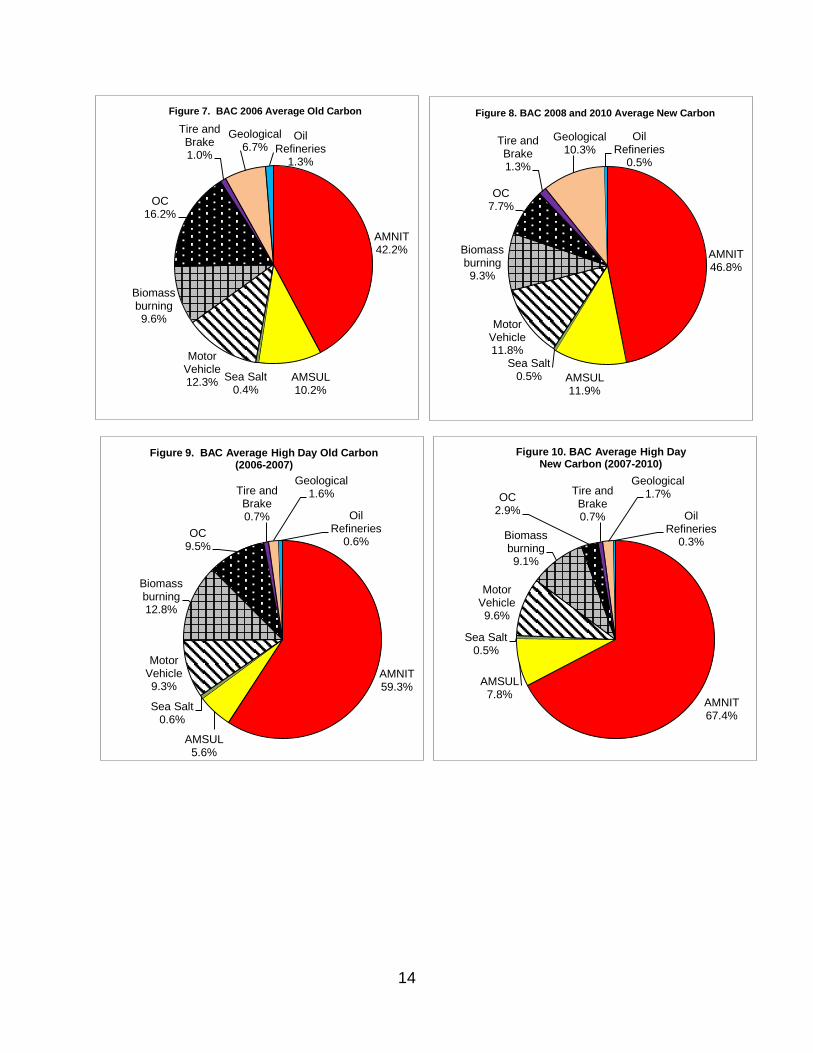
14

AMNIT 42.2%

AMSUL 10.2%

Sea Salt 0.4%

Motor Vehicle 12.3%

Biomass burning 9.6%

OC 16.2%

Tire and Brake 1.0%

Geological 6.7%

Oil Refineries

1.3%

Figure 7. BAC 2006 Average Old Carbon

AMNIT 59.3%

AMSUL 5.6%

Sea Salt 0.6%

Motor Vehicle 9.3%

Biomass burning 12.8%

OC 9.5%

Tire and Brake 0.7%

Geological 1.6%

Oil Refineries

0.6%

Figure 9. BAC Average High Day Old Carbon (2006-2007)

AMNIT 46.8%

AMSUL 11.9%

Sea Salt 0.5%

Motor Vehicle 11.8%

Biomass burning 9.3%

OC 7.7%

Tire and Brake 1.3%

Geological 10.3%

Oil Refineries

0.5%

Figure 8. BAC 2008 and 2010 Average New Carbon

AMNIT 67.4%

AMSUL 7.8%

Sea Salt 0.5%

Motor Vehicle 9.6%

Biomass burning 9.1%

OC 2.9%

Tire and Brake 0.7%

Geological 1.7%

Oil Refineries

0.3%

Figure 10. BAC Average High Day New Carbon (2007-2010)

15

Table 10. FSF Source Contribution (ug/m3)

Source Profile Annual Average High Days (>=30 ug/m3)

Name 2006-2008 2010 2006-2009 2009-2010

# of samples Obs Count 275

105

67

22 Mconc Mconc 20.3 ± 1.1 14.2 ± 0.8 46.3 ± 2.3 40.6 ± 2.1

Cconc Cconc 19.0 ± 1.5 10.8 ± 0.8 43.0 ± 2.9 33.1 ± 2.3

Rsquare Rsquare 0.8

0.9

0.9

0.9 CHIsquare CHIsquare 4.3

3.5

1.7

1.4

%MASS %MASS 96.7

74.3

92.9

81.5 AMNIT AMNIT 7.5 ± 0.7 4.7 ± 0.5 22.4 ± 2.1 17.8 ± 1.7

AMSUL AMSUL 1.7 ± 0.5 1.2 ± 0.4 2.1 ± 1.1 2.0 ± 1.0

Biomass burning Seasonal* 3.1 ± 0.5 1.7 ± 0.3 8.0 ± 1.2 7.6 ± 1.1

Motor Vehicle FGASDI** 2.1 ± 0.9 1.4 ± 0.5 4.0 ± 1.5 3.8 ± 1.3

OC OC 3.3 ± 1.1 1.0 ± 0.5 5.7 ± 2.0 1.5 ± 1.3

Tire and Brake TireBrk 0.1 ± 0.1 0.1 ± 0.1 0.2 ± 0.1 0.2 ± 0.1

Sea Salt MARINE75 0.1 ± 0.1 0.1 ± 0.1 0.2 ± 0.2 0.2 ± 0.2

Geological FDFREANN 0.8 ± 0.2 0.6 ± 0.1 0.2 ± 0.2 0.1 ± 0.1

Oil Combustion CHCRUC 0.01 ± 0.0

0.1 ± 0.0 0.0 ± 0.0

Table 11. FSF Source Contribution (%)

Source Profile Annual Average High Days (>=30 ug/m3) Name 2006-2008 2010 2006-2009 2009-2010 # of samples Obs Count 275 105 67 22 AMNIT AMNIT 40.0 43.2 52.0 53.6 AMSUL AMSUL 9.1 11.4 4.9 6.0 Biomass burning WBOakEuc 16.5 15.7 18.7 22.9 Motor Vehicle F9GASDI 11.1 13.3 9.3 11.5 OC OC 17.5 9.2 13.4 4.4 Tire and Brake TireBrk 0.8 0.8 0.5 0.5 Sea Salt MARINE75 0.6 0.9 0.5 0.7 Geological FDFREANN 4.2 5.6 0.5 0.3 Oil Combustion CHCRUC 0.1 0.0 0.1 0.0 * AgBWheat from June through October, WBoakEuc the rest of the year ** F6GASDIE for old carbon and F9GASDIE for new carbon

16

Contributions on individual exceedance days are illustrated in Figures 15 through 18. The highest contribution from each source is also summarized in Tables 12 and 13.

AMNIT 40.0%

AMSUL 9.1% Sea Salt

0.6%

Motor Vehicle 11.1%

Biomass burning 16.5%

OC 17.6%

Tire and Brake 0.8%

Geological 4.2%

Figure 11. FSF 2006-2008 Average Old Carbon

AMNIT 52.7%

AMSUL 4.9%

Sea Salt 0.5%

Motor Vehicle 11.8%

Biomass burning 24.5%

OC 4.6%

Tire and Brake 0.5%

Geological 0.4% Oil

Refineries 0.1%

Figure 13. FSF Average High Day Old Carbon (2006-2009)

AMNIT 43.2%

AMSUL 11.4% Sea Salt

0.9%

Motor Vehicle 13.3%

Biomass burning 15.7%

OC 9.2%

Tire and Brake 0.8%

Geological 5.6%

Figure 12. FSF 2010 Average New Carbon

AMNIT 53.6%

AMSUL 6.0%

Sea Salt 0.7%

Motor Vehicle 11.5%

Biomass burning 22.9%

OC 4.4%

Tire and Brake 0.5%

Geological 0.3%

Figure 14. FSF Average High Day New Carbon (2009-2010)

17

0102030405060708090

1001/

5/06

1/8/

06

1/11

/06

1/23

/06

2/4/

06

2/7/

06

2/10

/06

2/13

/06

10/2

/06

11/1

/06

11/7

/06

11/1

6/06

11/1

9/06

12/4

/06

12/7

/06

12/1

3/06

12/2

5/06

12/3

1/06

1/3/

07

1/9/

07

1/18

/07

1/21

/07

1/24

/07

1/27

/07

1/30

/07

2/2/

07

2/5/

07

2/8/

07

2/17

/07

Con

cent

ratio

ns (u

g/m

3)

Figure 15. PM2.5 Source Contribution on High Days 2006-2007 Bakersfield, Old Carbon

Oil Refining

Other OC

Biomass Burning

Motor Vehicle

Ammonium Sulfate

Ammonium Nitrate

Airborne Soil

Tires&Brakes

Sea Salt

PM2.5 Mass

0

10

20

30

40

50

60

70

80

10/2

7/07

11/2

/07

11/8

/07

11/1

4/07

11/2

6/07

11/2

9/07

12/1

1/07

12/1

4/07

12/2

3/07

1/10

/08

1/13

/08

1/16

/08

1/19

/08

2/9/

082/

12/0

82/

18/0

82/

27/0

83/

7/08

10/2

7/08

11/8

/08

11/1

7/08

11/2

0/08

11/2

6/08

12/1

1/08

11/3

/09

11/2

4/09

11/2

7/09

12/3

/09

12/2

1/09

12/2

7/09

1/5/

102/

4/10

11/4

/10

12/1

/10

12/4

/10

12/1

0/10

Con

cent

ratio

ns (u

g/m

3)

Figure 16. PM2.5 Source Contribution on High Days 2007-2010 Bakersfield, New Carbon

Oil Refining

Other OC

Biomass Burning

Motor Vehicle

Ammonium Sulfate

Ammonium Nitrate

Airborne Soil

Tires&Brakes

Sea Salt

PM2.5 Mass

18

0102030405060708090

100

1/5/

061/

11/0

61/

17/0

61/

23/0

62/

1/06

2/10

/06

2/13

/06

2/22

/06

10/2

/06

11/1

/06

11/1

6/06

11/2

2/06

11/2

5/06

12/1

/06

12/4

/06

12/7

/06

12/1

3/06

12/2

5/06

12/3

1/06

1/3/

071/

9/07

1/15

/07

1/18

/07

1/21

/07

1/24

/07

1/27

/07

1/30

/07

2/2/

072/

8/07

2/17

/07

11/2

/07

11/5

/07

11/8

/07

11/1

4/07

11/2

3/07

11/2

6/07

11/3

0/07

12/1

1/07

12/1

4/07

12/2

3/07

12/2

9/07

1/1/

081/

10/0

81/

13/0

81/

16/0

81/

19/0

82/

9/08

2/12

/08

2/18

/08

3/7/

0811

/8/0

811

/14/

0811

/26/

0811

/29/

0812

/5/0

812

/8/0

812

/11/

0812

/29/

081/

1/09

1/4/

091/

10/0

91/

13/0

91/

16/0

91/

19/0

91/

22/0

91/

28/0

91/

31/0

9

Con

cent

ratio

ns (u

g/m

3)

Figure 17. PM2.5 Source Contribution on High Days 2006-2009 Fresno, Old Carbon

Other OC

Biomass Burning

Motor Vehicle

Ammonium Sulfate

Ammonium Nitrate

Airborn Soil

Tires&Brakes

Sea Salt

PM2.5 Mass

0

10

20

30

40

50

60

70

11/1

2/09

11/1

5/09

11/2

4/09

12/3

/09

12/6

/09

12/9

/09

12/2

1/09

12/2

4/09

12/3

0/09

1/2/

10

1/8/

10

1/11

/10

1/15

/10

2/4/

10

2/19

/10

11/1

3/10

11/1

6/10

11/2

5/10

12/4

/10

12/7

/10

12/1

0/10

12/1

3/10

Con

cent

ratio

ns (u

g/m

3)

Figure 18. PM2.5 Source Contribution on High Days 2009-2010 Fresno, New Carbon

Other OC

Biomass Burning

Motor Vehicle

Ammonium Sulfate

Ammonium Nitrate

Airborn Soil

Tires&Brakes

Sea Salt

PM2.5 Mass

19

Table 12. BAC Highest Contribution by Source

Source Old Carbon New Carbon Contribution (ug/m3) Date Contribution (ug/m3) Date

Ammonium Nitrate 60 2/5/07 50 2/12/08 Ammonium Sulfate 5 10/2/06 11 1/5/10 Biomass Burning 18 12/25/06 12 11/29/07 Motor Vehicle 12 12/25/06 7 1/19/08 Other OC 9 2/5/07 5 2/12/08 Tire & Brake 0.6 1/24/07 0.8 12/4/10 Sea Salt 1 11/16/06 0.7 11/26/08 Geological 2.5 11/24/07 2.5 11/8/07 Oil Combustion 1 11/24/07 1 11/8/07

Table 13. FSF Highest Contribution by Source

Source Old Carbon New Carbon Contribution (ug/m3) Date Contribution (ug/m3) Date

Ammonium Nitrate 50 12/14/07 38 12/4/10 Ammonium Sulfate 5 12/23/07 7 1/8/10 Biomass Burning 21 1/1/08 19 11/25/10 Motor Vehicle 8 12/4/06 8 11/25/10 Other OC 13 1/19/08 6 12/24/09 Tire & Brake 0.6 12/7/06 0.4 11/24/09 Sea Salt 0.6 2/9/08 0.4 12/10/10 Geological 1.4 11/8/07 0.6 12/4/10 Oil Combustion 2 2/8/07

References

Chow, J.C., Watson, J. G., Lowenthal, D. H., and Countess, R. J.: Sources and chemistry of PM10 aerosol in Santa Barbara County, CA, Atmospheric Environment, 30, 1489-1499, 1996.

Chow, J.C., Watson, J.G., Crow, D., Lowenthal, D. H., and Merrifield, T.: Comparison of IMPROVE and NIOSH carbon measurements. Aerosol Science and Technology. 34:23-34, 2001.

Chow, J.C., Watson, J.G., Ashbaugh, L. L., and Magliano, K. L.: Similarities and differences in PM10 chemical source profiles for geological dust from the San Joaquin Valley, California. Atmospheric Environment. 37 (9-10):1317-1340, 2003.

20

Chow, J. C., Chen, L.-W. A., Lowenthal, D. H., Doriswamy, P., Park, K., Kohl, S., Trimble, D. L., and Watson, J. G.: California Regional PM10/PM2.5 Air Quality Study (CRPAQS) – Initial data analysis of field program measurements, California Air Resources Board, Sacramento, CA, by Desert Research Institute, Reno, NV, 2005.

Fitz, D. R. and Chow, J. C.: Development of gas and particulate matter organic profile database – draft work plan. Prepared for the San Joaquin Valleywide Air Pollution Study Agency, California Air Resourced Board. Sacramento, CA, by the University of California CE-CERT, Riverside, CA, 2001.

Fujita. E. M., Campbell, D., Zielinska, B., and Chow, J. C.: Kansas City PM Characterization Study, Round 1 Testing Report – Addendum A, Chemical Speciation, prepared for the U.S. Environmental Protection Agency, Desert Research Institute, Reno, NV, 2005.

21

Appendix A

Summary of Geological Profiles Used in CMB Modeling

Source Type Subtype County Sample ID Source FDKERANN Agricultural Soil Kern Soil 31 Houck, et al, 1989

Paved Road Urban Kern FDPVR1 Central California Fugitive Dust Study Animal

Husbandry Feedlot

(Composite) Kern&Fresno FDCTF

Unpaved Road Dust

Unpaved Parking lot

Kern Soil 13 Houck, et al, 1989

FDFREANN Paved Road Fresno Soil 03 Houck, et al, 1989

Agricultural Soil Almonds (Composite)

Kern, Fresno, King, and Madera

FDALM Central California Fugitive Dust Study

Agricultural Soil Grapes Fresno FDGRA1 Agricultural Soil Tomato

(Composite) Fresno FDTOM1

1

San Joaquin Valley PM2.5 Weight of Evidence Analysis

Appendix 3

Source Apportionment of PM2.5 Measured at the Fresno and Bakersfield Chemical Speciation Network Sites in San Joaquin Valley

Using the Positive Matrix Factorization Model

2

Source Apportionment of PM2.5 Measured at the Fresno and Bakersfield Chemical Speciation Network Sites in San Joaquin Valley

Using the Positive Matrix Factorization Model Sample Collection and Data Screening PM2.5 chemical speciation samples were collected on a one-in-three day schedule at the Fresno-First St. and Bakersfield-California Ave. Chemical Speciation Network (CSN) monitoring sites located in the San Joaquin Valley (SJV). There were good agreements between PM2.5 data collected by the speciation samplers and the collocated Federal Reference Method (FRM) samplers in matched Fresno data (340 samples, slope = 1.00, Intercept = 1.08, r2 = 0.97) and Bakersfield (175 samples, slope = 0.94, Intercept = 0.92, r2 = 0.94) between 2008 and 2010. The Thermal Optical Transmittance (TOT) protocol had been used to analyze carbon mass collected on the quartz filters. This method was changed to the Thermal Optical Reflectance (TOR) protocol and TOR organic carbon (OC) and elemental carbon (EC) concentrations were available starting from January 2008 and April 2009 at the Bakersfield and Fresno monitoring sites, respectively. Only the speciation data for which TOR OC and EC concentrations were available were considered in this source apportionment study. Since a carbon denuder that minimizes the positive sampling artifact caused by adsorption of gaseous organic materials was not included upstream of quartz filter in the CSN samplers, and none of the reported CSN data were blank corrected, an integrated OC artifact concentration that includes OC adsorption and desorption was estimated utilizing the intercept of the regression of OC concentrations against PM2.5 mass concentrations (Tolocka et al. 2001, Kim et al. 2005). Samples for which PM2.5 or OC concentrations had an error flag and samples for which the PM2.5 or OC data were not available were excluded from the regression analysis between PM2.5 and OC concentrations. Comparing co-located PM2.5 data measured by CSN and FRM samplers, and comparing PM2.5 and Sulfur (S) concentrations, outliers were censored for the two data sets. Using 189 data points out of 353 data points between 2009 and 2010 at Fresno and 187 data points out of 192 data points at Bakersfield between 2008 and 2010, the intercept s of 0.576 µg/m3 and 1.480 µg/m3 in PM2.5 regression against OC concentrations are considered to be the integrated OC artifact concentrations at Fresno and Bakersfield, respectively (Figure 1). The OC concentrations analyzed in this study were corrected by subtracting the integrated OC artifact concentrations.

3

Fresno-First St.

Bakersfield-California Ave.

Figure 1. OC artifact estimations: PM2.5 concentrations versus OC concentrations.

4

The Positive matrix factorization model version 2 (PMF2) model was used for the source apportionment of PM2.5 at the Fresno and Bakersfield monitoring sites. Samples were excluded from the data set for which the PM2.5, artifact corrected OC, or EC data were not available or below zero, or for which PM2.5 artifact corrected OC, or EC had an error flag. Samples for which the sum of all measured species were larger than twice the PM2.5 concentrations or the sum of all measured species were less than 50% of PM2.5 concentrations were also excluded. Finally, samples that contain fireworks particles collected on Independence Day and New Year’s Day were excluded since they had unusually high concentrations of OC, EC, K+, Na+ and metals. Overall, 10.3% of the Fresno data and 16.5% of the Bakersfield data were excluded in this study. For the chemical species screening, X-Ray Fluorescence (XRF) S was excluded from the analyses to prevent double counting of mass concentrations. Due to the higher analytical precision compared to XRF Na and XRF K, IC Na+ and IC K+ were included in the analyses. Chemical species below MDL values more than 90% were excluded. As recommended by Paatero and Hopke (2003), the species that had a Signal-to-Noise (S/N) ratio below 0.2 were excluded. Thus, a total of 174 samples and 21 species including PM2.5 mass concentrations collected between April 2009 and December 2010 were used for the Fresno site. For the Bakersfield site, a total of 147 samples and 24 species including PM2.5 mass concentrations collected between January 2008 and December 2010 were used. Since new TOR OC and EC concentrations were not accompanied by detection limit and uncertainty values, a comprehensive set of uncertainty structure (i.e., 7% of measured concentration) estimated by Kim et al. (2005) and 0.1 µg/m3 of detection limit value estimated from the State and Local Air Monitoring Stations (SLAM) speciation data were used in this study. Summaries of PM2.5 speciation data are provided in Tables A1 and A2 in the Appendix. The procedure of Polissar et al. (1998) was used to assign input data for PMF2. The measurement values are used for the input concentration data, and the sum of the analytical uncertainty and one-third of the detection limit value is used as the input uncertainty data assigned to each measured value. Concentration values below the detection limit are replaced by half of the detection limit values, and their input uncertainties are set at five-sixth of the detection limit values. Missing values are replaced by the geometric mean of the measured values for each species. To down-weight these replaced data and then to reduce their influence on the solution, their accompanying uncertainties are set at four times the geometric mean value. The conditional probability function (CPF) analysis was used to estimate the possible directions of the local source impacts (Kim and Hopke, 2004). The CPF was calculated for each source using the PMF2 source contributions coupled with wind data. As recommended by Paatero and Hopke (2003), which is to down-weight the variable in the analysis so that the noise does not compromise the solution, it was found necessary to increase the input uncertainties of OC, EC, and Cl by a factor of 3 for the Fresno data and OC and Na+ by a factor of 3 for the Bakersfield data to obtain physically interpretable PMF2 results.

5

PMF Results Seven major sources were resolved from PMF2 analyses for both sites (matrix rotational parameter: Fresno FPEAK = 0.1; Bakersfield FPEAK = 0). The comparison of the reconstructed PM2.5 contributions (sum of contributions from all sources) with measured PM2.5 concentrations shown in Figure 2 indicates that the resolved sources effectively reproduce the measured values and account for most of the variation in the PM2.5 concentrations (slope = 0.88, r2 = 0.95 for Fresno data; slope = 0.93, r2 = 0.91 for Bakersfield data). Average Source Contributions As shown in Figure 3 and Table A3 which present average source contributions, secondary nitrate contributed the most at both sites (35% at the Fresno site, 41% at the Bakersfield site). The pie charts indicate that three major sources (i.e., secondary nitrate, secondary sulfate, and motor vehicle) contributed 74% of PM2.5 concentrations at both sites. Figure 4 shows monthly average source contributions. Secondary nitrate, motor vehicle, and biomass smoke contributed the most in winter. The source profiles, corresponding source contributions, weekday/weekend variations, monthly averaged source contributions, and potential source directions are presented in Figures A1 through A10 in the Appendix. The secondary nitrate factor was identified by its high concentration of NO3

- and NH4

+. It consisted of NH4NO3 and several minor species such as secondary OC and EC that transport together. It contributed the most at both sites, accounting for 35% and 41% of the PM2.5 mass concentrations at Fresno and Bakersfield, respectively. Bakersfield showed higher secondary nitrate concentrations than Fresno. Secondary nitrate particles had winter- high trends at both sites. Secondary sulfate was identified by its high concentration of SO4

2- and NH4+ and accounted for 27% and 20% of the

PM2.5 mass concentration at Fresno and Bakersfield, respectively. Secondary nitrate and secondary sulfate did not show clear weekday/weekend variations. Secondary sulfate showed seasonal variations with higher concentrations in summer when the photochemical activity was highest at both sites. The CPF plots for secondary nitrate pointed S and NE at both sites. The CPF plots for secondary sulfate pointed SE at the Fresno site and SW at the Bakersfield site. The motor vehicle factor was identified by its high concentration of OC, EC, NO3

-, and minor species such as Fe (Watson et al., 1994). Motor vehicle emissions contributed 12% and 13% of the PM2.5 mass concentrations at Fresno and Bakersfield, respectively. Motor vehicle emissions did not show clear weekday/weekend variations at either site, however there was a winter-high seasonal trend.

6

The biomass smoke factor was characterized by OC, EC, and K+ (Watson et al., 2001) and contributed 11% and 10% to the PM2.5 mass concentrations at Fresno and Bakersfield, respectively. The biomass smoke category reflects contributions from residential wood burning and smoke from commercial cooking. The biomass smoke did not show weekday/weekend variations. The biomass smoke did show winter-high trends suggesting that it was mostly contributed by residential wood burning. The CPF plots for the biomass smoke pointed to high contributions from NE and S at both sites.

7

Fresno-First St.

Bakersfield-California Ave. Figure 2. Measured versus PMF predicted PM2.5 mass concentrations.

8

Figure 3. Average source contributions.

Figure 4. Monthly average source contributions.

9

The airborne soil factor was identified by its high concentrations of Si, Al, Ca and Fe. It contributed 7% and 10% to the PM2.5 mass concentration at Fresno and Bakersfield, respectively. Airborne soil reflects wind-blown dust as well as re-suspended crustal materials by road traffic as indicated by the presence of OC or EC in the source profiles. Airborne soil did not show clear weekday/weekend variation. Both sites exhibited autumn-high seasonal trends. The CPF plots for airborne soil suggested high contributions from SW and S at both sites. The aged sea salt factor was represented by its high concentrations of NO3

-, SO4

2-, and Na+, accounting for 6% the PM2.5 mass concentration at Fresno and 4% at Bakersfield. Aged sea salt reflects particles in which Cl- in the fresh sea salt is partially displaced by acidic gases during the transport and collected along with NO3

- and SO42-

(Song and Carmichael, 1999). Aged sea salt did not show weekday/weekend variation at either site. Aged sea salt had high contributions in summer at the Fresno site. Interestingly, it had a high contribution in winter at the Bakersfield site. The CPF plot for aged sea salt at Fresno site pointed towards NE. The CPF plot for aged sea salt at Bakersfield site suggested high contributions from NE and S. A possible industrial source such as metal processing that was characterized by OC, EC, Fe, and Zn was identified at both sites. This source accounted for 2% of the PM2.5 mass concentrations at both sites. It showed weak weekday-high variations at the Bakersfield site. The industrial source showed winter-high variations at the Fresno site. The CPF plot suggested high contributions from NE and SW at both sites.

Figure 5. Average source contributions in Fresno – First St. and Bakersfield – California Ave. when PM2.5 concentrations were higher than 30 µg/m3 in the high PM2.5 season (Nov. - Feb.).

10

Higher PM2.5 Day Contributions The average source contributions when PM2.5 concentrations were higher than 30 µg/m3 in the high PM2.5 season (Nov. - Feb.) are shown in Figure 5 for percentiles and in Table A4 for mass concentrations. The contributions from secondary nitrate and motor vehicle were increased from 35% up to 54% and from 12% up to 23%, respectively, at the Fresno site. The biomass burning contributions also increased slightly from 11% up to 13% at Fresno site. At the Bakersfield site, the contributions from secondary nitrate increased from 41% up to 64% and aged sea salt from 4% up to 6%. Conclusions PM2.5 speciation and related meteorological data collected at the Fresno-First St. and Bakersfield-California Ave. CSN monitoring sites between 2008 and 2010 were analyzed by PMF2. Seven major PM2.5 sources were identified at both monitoring sites: secondary nitrate, secondary sulfate, motor vehicle, biomass smoke, airborne soil, aged sea salt, and industrial. Annual average and high day source contributions showed that secondary nitrate, secondary sulfate, motor vehicles, and biomass burning were the largest contributors to PM2.5 concentrations. References Kim, E., Hopke, P.K. Comparison between conditional probability function and

nonparametric regression for fine particle source directions, Atmospheric Environment 38, 11, 4667-4673, 2004.

Kim, E., Hopke, P.K. and Qin, Y. Estimation of organic carbon blank values and error structures of the speciation trends network data for source apportionments, Journal of Air and Waste Management Association 55, 1190–1199, 2005.

Paatero, P., Hopke, P.K. Discarding or downweighting high-noise variables in factor analytic models, Analytica Chimica Acta, 490, 277-289, 2003.

Polissar, A.V., Hopke, P.K., Paatero, P., Malm, W.C. and Sisler, J.F. Atmospheric Aerosol over Alaska 2. Elemental Composition and Sources, Journal of Geophysical Research, 103, 19045-19057, 1998.

Song, C.H., Carmichael, G.R. The aging process of naturally emitted aerosol (sea salt and mineral aerosol) during long-range transport, Atmospheric Environment 33, 2203-2218, 1999.

11

Tolocka, M.P., Solomon, P.A., Mitchell, W., Norris, G.A., Gemmill, D.B., Wiener, R.W., Vanderpool, R.W., Homolya, J.B. and Rice, J.East versus west in the US: Chemical characteristics of PM2.5 during the winter of 1999, Aerosol Science and Technology 34, 88-96, 1999.

Watson, J.G., Chow, J.C., Lowenthal, D.H., Pritchett, L.C. and Frazier, C.A. Differences in the carbon composition of source profiles for diesel and gasoline powered vehicles, Atmospheric Environment 28(15), 2493-2505, 1994.

Watson, J.G., J.C. Chow, and J.E. Houck, PM2.5 chemical source profiles for vehicle exhaust, vegetative burning, geological material, and coal burning in northwestern Colorado during 1995, Chemosphere, 43, 1141-1151, 2001.

12

APPENDIX Table A1. Summary of PM2.5 species mass concentrations at Fresno.

Species Arithmetic

mean (µg/m3)

Geometric mean

(µg/m3)

Minimum (µg/m3)

Maximum (µg/m3)

Number of below MDL values (%)

PM2.5 14.5649 11.2762 0.3000 66.6000 0.6

OC 2.7861 1.9428 0.1600 17.4240 0.0

EC 0.7934 0.5764 0.0769 5.0400 0.6

SO4 1.2507 1.1155 0.2440 5.3900 0.6

NO3- 3.6499 1.9445 0.0445 29.1000 0

NH4+ 1.3964 0.8936 0.1380 9.3500 0.6

Al 0.0646 0.0418 0.0013 0.6330 25.3

Br 0.0042 0.0032 0.0001 0.0338 15.5

Ca 0.0420 0.0310 0.0027 0.2860 4.0

Cl 0.0563 0.0156 0.0001 0.5130 40.2

Cr 0.0026 0.0018 0.0000 0.0387 75.3

Cu 0.0044 0.0032 0.0001 0.0163 28.7

Fe 0.1007 0.0843 0.0129 0.6890 0

K+ 0.1072 0.0770 0.0169 0.6460 32.8

Mg 0.0200 0.0138 0.0002 0.1140 68.4

Mn 0.0019 0.0015 0.0000 0.0126 62.1

Na+ 0.1373 0.0972 0.0176 0.8720 3.4

Ni 0.0074 0.0017 0.0000 0.1850 65.5

Si 0.1682 0.1100 0.0006 1.6400 1.7

Ti 0.0057 0.0043 0.0001 0.0448 61.5

Zn 0.0067 0.0045 0.0004 0.0296 25.3

13

Table A2. Summary of PM2.5 species mass concentrations at Bakersfield.

Species Arithmetic

mean (µg/m3)

Geometric mean

(µg/m3)

Minimum (µg/m3)

Maximum (µg/m3)

Number of below MDL values (%)

PM2.5 20.9253 17.1631 2.9000 73.3000 0

OC 2.4981 1.7591 0.0400 18.2200 1.3

EC 1.1390 0.9764 0.2160 3.0900 0

SO4 1.6927 1.4718 0.1200 8.0600 0

NO3- 6.4908 3.2626 0.3520 35.7000 0

NH4+ 2.5874 1.5187 0.3160 14.8000 0.7

Al 0.1276 0.0818 0.0013 1.0800 12.7

As 0.0015 0.0013 0.0001 0.0056 73.3

Br 0.0058 0.0048 0.0001 0.0299 4.7

Ca 0.1096 0.0791 0.0065 0.6770 1.3

Cl 0.0436 0.0192 0.0002 0.3270 26.0

Co 0.0013 0.0010 0.0000 0.0047 76.0

Cr 0.0021 0.0016 0.0001 0.0156 80.0

Cu 0.0089 0.0064 0.0002 0.0570 10.0

Fe 0.1923 0.1555 0.0020 1.0900 0

K+ 0.1091 0.0931 0.0183 0.5280 16.0

Mg 0.0238 0.0160 0.0002 0.2310 60.7

Mn 0.0034 0.0025 0.0003 0.0276 32.7

Na+ 0.1556 0.1229 0.0168 0.6980 1.3

Ni 0.0010 0.0009 0.0000 0.0042 84.7

Si 0.3586 0.2322 0.0217 3.4300 0.7

Sr 0.0019 0.0017 0.0001 0.0120 84.0

Ti 0.0103 0.0068 0.0001 0.0818 46.7

Zn 0.0127 0.0084 0.0006 0.1300 8.7

14

Table A3. Average source contributions (µg/m3) to PM2.5 mass concentration.

Sources Average source contribution (± 95 % distribution)

Fresno Bakersfield

Secondary nitrate 4.89 (1.09) 8.07 (1.85)

Secondary sulfate 1.72 (0.16) 2.60 (0.39)

Motor vehicle 3.70 (0.44) 4.01 (0.39)

Biomass smoke 1.47 (0.28) 2.02 (0.28)

Airborne soil 0.83 (0.14) 1.97 (0.37)

Aged sea salt 1.04 (0.16) 0.79 (0.22)

Industrial 0.22 (0.03) 0.40 (0.11)

Estimated PM2.5 (µg/m3) 13.86 (1.57) 19.85 (2.27)

Measured PM2.5 (µg/m3) 14.56 (1.74) 20.48 (2.33)

15

Table A4. Average source contributions (µg/m3) to PM2.5 mass concentration at Fresno-First St. and Bakersfield-California Ave. when PM2.5 mass concentrations were higher than 30 µg/m3 between Nov. and Feb.

Sources Average source contribution (Nov. – Feb.)

Fresno Bakersfield

Secondary nitrate 20.14 28.83

Secondary sulfate 2.42 3.80

Motor vehicle 8.58 5.69

Biomass smoke 4.87 2.83

Airborne soil 0.18 0.71

Aged sea salt 0.47 2.52

Industrial 0.35 0.38

No. of days 21 25

16

Figure A1. Source profiles deduced from PM2.5 samples measured at Fresno-First St. (prediction ± standard deviation).

17

Figure A2. Source profiles deduced from PM2.5 samples measured at Bakersfield-California Ave. (prediction ± standard deviation).

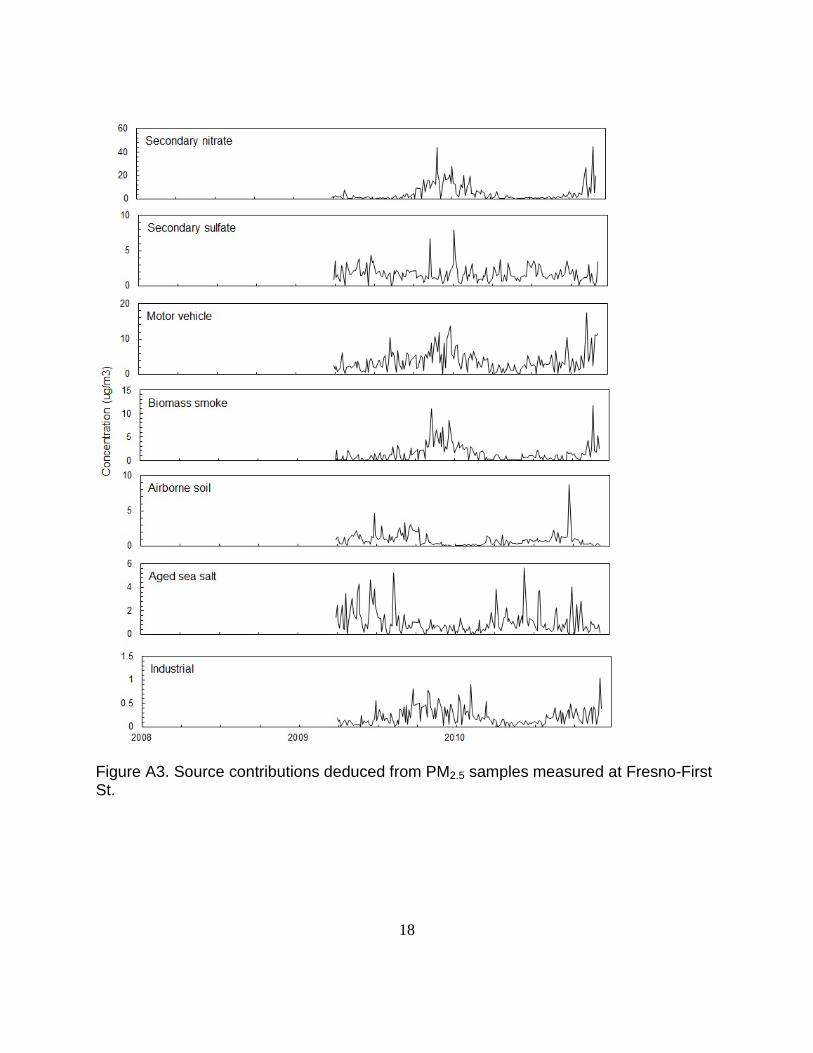
18

Figure A3. Source contributions deduced from PM2.5 samples measured at Fresno-First St.

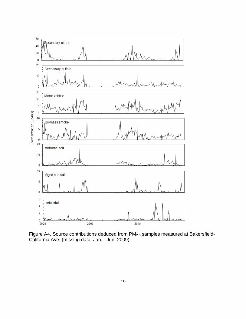
19

Figure A4. Source contributions deduced from PM2.5 samples measured at Bakersfield-California Ave. (missing data: Jan. - Jun. 2009)

20

Figure A5. Weekday/weekend variations at Fresno-First St. (mean ± 95 % distribution).

21

Figure A6. Weekday/weekend variations at Bakersfield-California Ave. (mean ± 95 % distribution).

22

Figure A7. The monthly variations of source contributions to PM2.5 mass concentration at Fresno-First St. (mean ± 95 % distribution).

23

Figure A8. The monthly variations of source contributions to PM2.5 mass concentration at Bakersfield-California Ave. (mean ± 95 % distribution).

24

Secondary nitrate

Figure A9. Conditional probability function plots for the highest 25% of the mass contributions at Fresno-First St.

25

Secondary nitrate

Figure A10. Conditional probability function plots for the highest 25% of the mass contributions at Bakersfield-California Ave.

1

San Joaquin Valley PM2.5 Weight of Evidence Analysis

Appendix 4

Methodology for Meteorological Adjustment of PM2.5 Trend Statistics

2

Introduction

Air quality trends can help reveal the effects of emission control strategies and regulations on ambient air pollution levels. However, meteorological conditions also affect pollutant levels and can obscure the effects of changing emissions on ambient air pollution levels over time. If the met-effects can be identified, quantified, and removed, the met-adjusted trends may reveal the emissions-induced trends with greater clarity.

For the San Joaquin Valley PM2.5 SIP, met-adjusted trends were prepared for annual average PM2.5 and for PM2.5 exceedance days. This Technical Appendix presents the methodology used to construct the met-adjusted trends.

1. Data Acquisition and Preparation

PM2.5 mass concentrations from the air quality monitoring sites in two major urban centers of the SJV (Bakersfield and Fresno) were collected. Meteorological data for factors that may impact the PM2.5 concentrations were also acquired from various meteorological monitoring networks. Monitors at ground level provided temperature, relatively humidity, pressure, wind speed, wind direction, precipitation, and solar radiation data. For various reasons, surface pressure, wind direction, precipitation, and solar radiation were not used in the final analysis. Routine rawinsondes (weather balloons) at Oakland provided data for 500 millibar heights and 850 millibar temperatures. These surface and upper air factors are consistent with studies of meteorological conditions associated with daily PM2.5 levels [Dye et al., 2003].

Table 1 lists the air quality and meteorological monitoring sites that provided data used in this analysis. The PM2.5 and meteorological data presented are daily regional averages of the data collected from the sites in Table 1.

Table 1. Air quality and meteorological monitoring sites

Region Air Quality Sites Meteorological Sites

Bakersfield Area

Bakersfield-Golden State Highway, Bakersfield-5558 California Avenue, Bakersfield-410 E Planz Road

Oakland (Upper Air), Mercury/Desert Rock (Upper Air), Vandenberg AFB (Upper Air), Bakersfield-Golden State Highway, Bakersfield-5558 California Avenue, Oildale-3311 Manor Street, Shafter-Walker Street, Arvin-Edison, Belridge

Fresno Area Fresno-1st Street, Clovis-N Villa Avenue Fresno-Hamilton and Winery

Oakland (Upper Air) Fresno-1st Street Clovis-N Villa Avenue,

A consistent analysis of met-effects on daily PM2.5 will benefit from and may require the presence of all PM2.5 and meteorological data for each daily record used in the analysis. If any values are missing, the entire day might be excluded from further consideration. Therefore, data completeness is very desirable for the analysis to be as meaningful as possible. To minimize instances of missing PM2.5 and meteorological

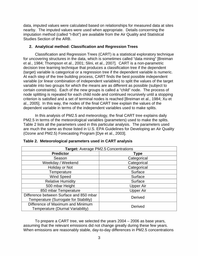
3

data, imputed values were calculated based on relationships for measured data at sites nearby. The imputed values were used when appropriate. Details concerning the imputation method (called “I-Bot”) are available from the Air Quality and Statistical Studies Section of the ARB.

2. Analytical method: Classification and Regression Trees

Classification and Regression Trees (CART) is a statistical exploratory technique for uncovering structures in the data, which is sometimes called “data mining” [Breiman et al., 1984; Thompson et al., 2001; Slini, et al., 2007]. CART is a non-parametric decision tree learning technique that produces a classification tree if the dependent (target) variable is categorical or a regression tree if the dependent variable is numeric. At each step of the tree building process, CART finds the best possible independent variable (or linear combination of independent variables) to split the values of the target variable into two groups for which the means are as different as possible (subject to certain constraints). Each of the new groups is called a “child” node. The process of node splitting is repeated for each child node and continued recursively until a stopping criterion is satisfied and a set of terminal nodes is reached [Breiman et al., 1984; Xu et al., 2005]. In this way, the nodes of the final CART tree explain the values of the dependent variable in terms of the independent variables used to make splits.

In this analysis of PM2.5 and meteorology, the final CART tree explains daily PM2.5 in terms of the meteorological variables (parameters) used to make the splits. Table 2 lists all the parameters used in this particular analysis. The parameters used are much the same as those listed in U.S. EPA Guidelines for Developing an Air Quality (Ozone and PM2.5) Forecasting Program [Dye et al., 2003].

Table 2. Meteorological parameters used in CART analysis

Target: Average PM2.5 Concentrations Predictor Type Season Categorical

Weekday / Weekend Categorical Holiday or Not Categorical Temperature Surface Wind Speed Surface

Relative Humidity Surface 500 mbar Height Upper Air

850 mbar Temperature Upper Air Difference between Surface and 850 mbar

Temperature (Surrogate for Stability) Derived

Difference of Maximum and Minimum Temperature (Diurnal Variability) Derived

To prepare a CART tree, we selected the years 2004 – 2006 as base years, assuming that the relevant emissions did not change greatly during these few years. When emissions are reasonably stable, day-to-day differences in PM2.5 concentrations

4

are mostly due to differences in meteorology. We then applied CART analysis to the base years to define a relationship (“tree”) between daily PM2.5 and daily meteorological conditions.

First, we forced the tree to be split by season so that an independent sub-tree was generated for each season. Each sub-tree consisted of one or more terminal nodes representing different meteorological classes. The CART system makes the differences in PM2.5 between the met-classes as large as possible and the differences in PM2.5 within the met-classes as small as possible. The PM2.5 concentration representing each met-class (terminal node) is the average concentration of all the days assigned to that met-class in the base years. For each day assigned to a met-class, the average PM2.5 for the met-class serves as a “predicted PM2.5” for that day. Days with high predicted values have met-conditions that are more conducive to PM2.5 formation compared to days with low predicted values.

The CART-defined relationships between meteorology and PM2.5 in the base years were then used to assign days in the other years to their appropriate met-classes based on their day-specific meteorological data. The predicted PM2.5 values for all the days are then used to adjust PM2.5 trends up or down to compensate for each year’s PM2.5-conduciveness relative to “normal”.

3. Results and Discussion

Based on daily air quality and meteorological data in 2004-2006, a CART tree with 17 met-classes (terminal nodes) was constructed for the Bakersfield area (Figure 1a) and a CART tree with 22 met-classes was constructed for the Fresno area (Figure 1b). Figure 2 indicates that ~75 – 80 percent of the variation in daily PM2.5 during the base years is accounted for by each of the CART trees. Table 3 shows that three met-factors – wind speed, stability (difference surface 850mb temperatures), and minimum surface temperature – affected daily PM2.5 concentrations strongly in both Bakersfield and Fresno, while relative humidity (RH) was more important for PM2.5 production in the Bakersfield area than in the Fresno area. In general, high PM2.5 concentrations in the Bakersfield were associated with relatively high stability, low wind speed and high RH. In Fresno, high PM2.5 was generally associated with cold mornings (low minimum surface temperature), high stability, and low wind speed.

It is worth mentioning that this CART model treats each day independently and does not directly characterize met-conditions over a sequence of days that may result in long-term buildup and transport of PM2.5.

A sensitivity analysis was, also, done to explore the impact of the selected base years on the CART results for the Bakersfield area. For this purpose, different sets of base years (2003-2005, 2004-2006, and 2006-2008) were used with CART to develop relationships between meteorology and PM2.5. The met-adjusted annual average PM2.5 concentrations proved to be quite similar regardless of the base years used in the CART analysis.

5

(a)

(b)

Figure 1. CART terminal nodes sorted by target variable predictions (PM2.5) in (a) Bakersfield area and (b) Fresno area.

20

40

60

80

BA

KE

RS

FIE

LD_P

M25

_AV

ER

AG

ETerminal Nodes Sorted By Target Variable Prediction

20

40

60

80

FRE

SN

O_A

VE

RA

GE

Terminal Nodes Sorted By Target Variable Prediction

6

(a)

(b)

Figure 2. Observations vs. CART predictions during the base years in the (a) Bakersfield and (b) Fresno areas

y = 1x + 5E-06R² = 0.7523

0102030405060708090

100

0 20 40 60 80 100

Obs

erve

d PM

2.5

at B

aker

sfie

ld

CART Predicted PM2.5 at Bakersfield Area

y = 1x - 5E-08R² = 0.789

0

10

20

30

40

50

60

70

80

90

0 10 20 30 40 50 60 70

Obs

erve

d PM

2.5

at F

resn

o Ar

ea

CART Predicted PM2.5 at Fresno Area

7

Table 3. Relative importance of met-factors in forming the CART trees on a 0 to 100 scale.

Annual average PM2.5 trends for observed data and for CART-predicted values (2004-2006 used as base years) were compared in the Bakersfield and Fresno areas. In both areas, observed PM2.5 levels decreased significantly from 1999 to 2003, were relatively flat from 2003 to 2008, then decreased in 2009 and 2010. CART-predicted trends represent meteorological conditions that affect PM2.5 concentrations. For the Bakersfield area, the CART-predicted trend indicates that met-conditions favored lower than normal PM2.5 in 1999 – 2000, normal PM2.5 from 2001 – 2006, and higher than normal PM2.5 from 2007 – 2010. The CART-predicted trend for the Fresno area indicates that met-conditions have been more stable and have had relatively small impacts on the observed PM2.5 trends from 1999 – 2010.

The CART-predicted trend information was merged with the observed trends to produce met-adjusted trends for annual average PM2.5. Figure 3 shows the observed and met-adjusted trends for (a) the Bakersfield area and (b) the Fresno area. Linear trend lines are shown for the observed and the met-adjusted trends in each area. Figure 3 indicates that the met-adjusted trend shows a greater decrease than the observed trend in the Bakersfield area, while the met-adjusted trend is similar to the observed trend in the Fresno area. In both areas, met-adjusted PM2.5 decreased by ~ 0.8 µg/m3 per year from 1999 – 2010. Overall, the met-adjusted trends indicate that average PM2.5 decreased 40 – 50 percent in the Bakersfield and Fresno areas from 1999 – 2010 as a consequence of ongoing emission reductions.

Meteorological Factor Variable Importance in Bakersfield Variable Importance in FresnoAverage Wind Speed 100 100

Aveage Surface T - 850 mbar T 69.02 56.24Minimum Surface Temperature 56.11 60.89

Season 52.52 51.48Minium Surface T - 850 mbar T 47.74 36.37

Maximum Surface T - 850 mbar T 45.59 96.49Average Relatively Humidity 40.12 10.11

Average Surface Temperature 39.84 59.65Maximum Surface Temperature 28.51 37.02

Afternoon 850 mbar Temperature 26.4 6Average 850 mbar Temperature 20.88 5.89

Average 500 mbar Height 12.42 22.91Afternoon 500 mbar Height 12.14 7.07Maximum Relative Humidity 10.45 9.67

Morning 850 mabr Temperature 6.01 5.85Maximum Surfact T - Minimum Surface T 4.15 3.76

Minimum Relative Humidity 3.54 2.84Morning 500 mbar Height 0.07 5.43

8

(a)

(b)

Figure 3. Trends of observed and meteorologically adjusted PM2.5 concentrations in (a) Bakersfield and (b) Fresno areas of the San Joaquin Valley

y = -0.56x + 1139.6R² = 0.62

y = -0.8x + 1623.7R² = 0.77

0

10

20

30

1998 1999 2000 2001 2002 2003 2004 2005 2006 2007 2008 2009 2010 2011

PM2.

5(µ

g/m

3 )

Year

Observed and Met-Adjusted Annual Average PM2.5 Trends in Bakersfield Area

Observed PM2.5Met-Adjusted PM2.5 in Bakersfield AreaLinear (Observed PM2.5)Linear (Met-Adjusted PM2.5 in Bakersfield Area)

y = -0.9x + 1820.5R² = 0.81

y = -0.8x + 1614.4R² = 0.74

0

10

20

30

1998 1999 2000 2001 2002 2003 2004 2005 2006 2007 2008 2009 2010 2011

PM2.

5(µ

g/m

3 )

Year

Observed and Met-Adjusted Annual Average PM2.5 Trends in Fresno Area

Observed PM2.5Met-Adjusted PM2.5Linear (Observed PM2.5)Linear (Met-Adjusted PM2.5)

9

Trends for exceedance days were prepared for the Bakersfield and Fresno sub-regions. For this work, an exceedance day meant that the sub-regional average daily PM2.5 concentration was greater than or equal to 35 ug/m3. Trends for the observed PM2.5 data and for the CART-predicted PM2.5 data (representing meteorological effects) were prepared.

In the Bakersfield area, similar to the annual averages, the CART-predicted exceedance days increased from the earlier years to recent years, indicating an increase in meteorological conduciveness for PM2.5. In the Fresno area, the impact of meteorology on PM2.5 exceedance days was relatively small, again similar to the annual averages. In both areas, the observed PM2.5 exceedance days were greater than the CART-predicted PM2.5 exceedance days from 1999 through 2002. The two trends were similar from 2003 through 2008. Finally, for 2009 and 2010, observed PM2.5 exceedance days decreased significantly and dipped below the CART-predicted exceedance days. The implication of these results is that emission reductions played a significant role in decreasing the PM2.5 exceedance days from 1999 – 2010, especially in the Bakersfield area.

The CART-predicted trend information was merged with the observed trends to produce met-adjusted trends for PM2.5 exceedance days. Figure 4 shows that after adjusting for meteorology, PM2.5 exceedance days decreased about 60 – 70 percent from 1999 to 2010, with decreases of ~ 3.5 days per year in the Fresno area and ~ 4.5 days per year in the Bakersfield area.

10

(a)

(b)

Figure 4. Trends of observed and meteorologically adjusted PM2.5 exceedance days in (a) the Bakersfield area and (b) the Fresno area.

y = -2.5x + 5117R² = 0.37

y = -4.5x + 8976R² = 0.73

0

30

60

90

1998 2000 2002 2004 2006 2008 2010 2012

PM2.

5Ex

ceed

ance

Day

s

Year

Observed and Met-Adjusted PM2.5 Exceedance Days in Bakersfield Area

Observed PM2.5 Exceedance Days in Bakersfield Area

Met-Adjusted PM2.5 Exceedance Days in Bakersfield Area

Linear (Observed PM2.5 Exceedance Days in Bakersfield Area)

Linear (Met-Adjusted PM2.5 Exceedance Days in Bakersfield Area)

y = -4.2x + 8449R² = 0.58

y = -3.5x + 7138R² = 0.50

0

30

60

90

1998 2000 2002 2004 2006 2008 2010 2012

PM2.

5Ex

ceed

ance

Day

s

Year

Observed and Met-Adjusted PM2.5 Exceedance Days in Fresno Area

Observed PM2.5 Exceedance Days in Fresno Area

Met-Adjusted PM2.5 Exceedance Days in Fresno Area

Linear (Observed PM2.5 Exceedance Days in Fresno Area)

Linear (Met-Adjusted PM2.5 Exceedance Days in Fresno Area)

11

4. Summary

Overall, CART analysis can help us to define the relationship between PM2.5 mass concentrations and meteorological conditions and to calculate meteorologically adjusted trends. Such trends can help reveal the impact of emission changes on air pollutant levels, and promote the development of effective air pollution control strategies and regulations. Of course, as with any statistical analysis, there are uncertainties and limitations in CART analysis. Therefore, caution is needed when interpreting the resulting air quality trends, especially when small differences occur within short time periods.

The annual average PM2.5 concentrations and the number of exceedances of the 24-hour PM2.5 standard followed similar trends in the Bakersfield and Fresno areas from 1999-2010. In the Fresno area, the meteorological conditions seem to have been relatively stable, so met-adjusted trends were similar to the observed trends. In the Bakersfield area, however, meteorological conditions were relatively less PM2.5 conducive in the earlier years (i.e. 1999-2000) and more conducive in recent years (i.e. 2007-2010), with more normal years in between. Accordingly, the met-adjusted trends for the Bakersfield area show a greater decrease in PM2.5 levels compared to the observed trends.

Based on the differences between the predicted PM2.5 levels under the observed meteorological conditions and under “normal” meteorological conditions, the PM2.5 observations are adjusted to derive met-adjusted PM2.5 trends. The analyses indicate that the met-adjusted annual average PM2.5 concentrations decreased at a rate of ~0.8 µg/m3 per year between 1999 and 2010 for a total of ~40-50 percent decrease in met-adjusted PM2.5 in the Bakersfield and Fresno areas as a result of emission reductions during this period. Met-adjusted trends for PM2.5 exceedance days indicate ~60-70 percent progress from 1999 – 2010, with decreases of ~ 3.5 days per year in the Fresno area and ~ 4.5 days per year in the Bakersfield area.

5. References

Breiman, L., J.H. Friedman, R.A. Olshen, C.J. Stone, Classification and regression trees, Wadsworth and Brooks/Cole, Monterey, 1984.

Dye, T.S., MacDonald, C.P., Anderson, C.B., Hafner, H.R., Wheeler, N.J.M., Chan, A.C., Guidelines for developing an air quality (ozone and PM2.5) forecasting program, EPA-456/R-03-002, Environmental Protection Agency, NC, U.S.A., 2003.

Slini, T., A. Kaprara, K. Karatzas, N. Moussiopoulos, PM10 forecasting for Thessaloniki, Greece, Environmental Modelling and Software, Volume 21, Issue 4, April 2006, Pages 559-565, ISSN 1364-8152, 10.1016/j.envsoft.2004.06.011, 2006.

12

Thompson, M. L., J. Reynolds, L. H. Cox, P. Guttorp, P. D. Sampson, A review of statistical methods for the meteorological adjustment of tropospheric ozone, Atmospheric Environment, Volume 35, Issue 3, Pages 617-630, ISSN 1352-2310, 10.1016/S1352-2310(00)00261-2, 2001.

Xu, M., P. Watanachaturaporn, P.K. Varshney, M.K. Arora, Decision tree regression for soft classification of remote sensing data. Remote Sensing of Environment 97, 322-336, 2005.