Chapter 5

Noise

At this point, we are able to evaluate the performance of a communication or radar link and estimate the amount ofpower we expect to receive. What is important for determining detectability, however, is not the absolute signal power(which can always be improved through amplification), but the signal to noise ratio (which cannot). We will see laterthat there are strategies for optimizing this ratio that constitute a significant fraction of the radar art. Below, we beginby investigating natural and instrumental noise sources.

5.1 Noise in passive linear networks

All the pertinent ideas were worked out in a 1928 Physical Review paper by H. Nyquist that still stands as a hallmark ofelegant, incisive reasoning (and writing). The simplest noise source, after which other noise sources can be modeled,is a resistor at finite temperature. Thermal agitation of thecharge carriers in the resistor causes a random signal toappear across its terminals. The signal is a Gaussian randomvariable in accordance with the central limit theorem,which governs the statistics of processes that depend on a large number of chance occurrences. The probability of agiven voltage being present in an infinitesimal voltage interval dv at any instant is

P (v)dv =1√

2πσv

e−v2/2σ2

vdv

which is normalized so that the total occurrence probability is unity, i.e.,∫

∞

−∞

P (v)dv = 1

and the random variablev has zero mean and varianceσ2v

σ2v = 〈v2〉 =

∫

v2P (v)dv

Thermal noise is broad-banded. The variance of the noise in abandwidth∆f Hz wide depends on the temperatureof the resistor according to Planck’s law:

σ2v(∆f) =

4hfR∆f

ehf/KT − 1

whereh is Planck’s constant (6.62 × 10−34 Js),K is Boltzmann’s constant (1.38 × 10−23 J/K), f is the frequency inHz,R is the resistance, andT is the Kelvin temperature. In the domain of radio frequencies and ‘normal’ temperatures,the exponential in the denominator can be approximated as1 + hf/KT , and the RMS noise voltage in the band∆fbecomes:

vRMS(∆f) = 2√

KTR∆f

79

R

~

T

v

Rl+jχlB=∆f

Figure 5.1: Illustration of Nyquist’s theorem. A resistorR is connected to a passive linear network (Zl = Rl + jχl)via a bandpass filter with bandwidthB = ∆f centered on frequencyf .

which is a statement of Nyquist’s theorem. Here,vRMS can be interpreted as the Thevenin equivalent noise voltagefor a resistor at temperatureT operating in a channel bandwidth∆f .

Nyquist’s theorem applies not only to resistors but to any passive linear network. The principle is illustratedin Figure 5.1. Consider a resistorR at temperatureT connected by means of a lossless bandpass filter centered atfrequencyf with bandwidthB = ∆f to a passive linear network with impedanceZl = Rl + jχl as shown. Accordingto Ohm’s law, the power delivered by the resistor to the network will be P=I2

RMSRl or

P =

∣∣∣∣

vRMS

R + Zl

∣∣∣∣

2

Rl

=4KTR∆f

|R + Zl|2Rl

The resistor and the network must eventually achieve thermodynamic equilibrium, at which point their temperatureswill be the same, and the power delivered from the network to the resistor will match the power delivered from theresistor to the network found above. This is the principle ofdetailed balance. Definev′ as the Thevenin equivalentnoise voltage of the network. Then the power delivered from the network to the resistor must be

P ′ =

∣∣∣∣

v′RMS

R + Zl

∣∣∣∣

2

R = P

Solving this equation forv′ yields

v′RMS(∆f) = 2√

KTRl∆f

which is Nyquist’s theorem generalized for any passive linear network with Thevenin equivalent resistanceRl.

In the event that the load is matched to the source,Rl = R, χl → 0, the power delivered by the noise source overthe bandwidth∆f is justP = KT∆f (W). This is the so-called available noise power under matched load conditions.This results is also referred to as Nyquist’s theorem and will be used throughout the rest of the chapter. (In the eventof an impedance mismatch, an extra factor of(1 − |Γ|2) should be included, whereΓ is the reflection coefficient.)For example, takingT = 300 K (room temperature) and considering a bandwidthB = 1 MHz gives a noise power of4× 10−15 W. This may seem like a very small amount of power, but it couldbe significant (even dominant) comparedto the signal power received directly from the terminals of an antenna, depending on the application.

5.2 Antenna noise temperature

Nyquist’s theorem applies only to passive linear devices. An antenna is such a device and so is governed by Nyquist’stheorem. However, the noise temperature of an efficient antenna is not usually related to the ambient temperature.Antennas are not ohmic (the radiation resistance is not the ohmic resistance), and the random signals on them aremainly due to something other than the thermal agitation of the charge carriers. Antennas are in radiative contact with

80

R,T

dΩ

T(θ,φ)

ν(θ,φ)

Figure 5.2: Diagram illustrating concept of antenna noise temperature.

bodies in their field of view, including bodies in the atmosphere and in space, and these radio sources almost alwaysdetermine the noise level/temperature of the antenna. The actual noise temperature depends strongly on frequency andalso on antenna pointing.

Figure 5.2 shows an antenna connected to a resistorR at temperatureT which serves as a signal source. The avail-able noise power delivered to the antenna, which is assumed to be matched to the resistor, isP = KT∆f . The powerradiated into the differential solid angledΩ in the direction(θ, φ) will consequently beP = KT∆f(D(θ, φ)/4π)δΩ.Within that solid angle is a body at temperatureT (θ, φ). Suppose that the fraction of the power absorbed by that bodyis ν(θ, φ). If the resistor and the body were in thermodynamic equilibrium, that is, the only heat source for the body(cloud) is the radiating antenna, the body and the resistor would have the same temperature, and the amount of powerreceived from the body and delivered to the resistor would equal the amount of power radiated from the resistor andabsorbed by the body:

Pr = K∆fD(θ, φ)

4πν(θ, φ)T (θ, φ)dΩ

In fact, we do not expect the resistor and the body to be in thermodynamic equilibrium. Nevertheless, this formulashould hold for arbitrary bodies at any temperatureT (θ, φ) in the antenna field of view. Note that this discussionimplies that perfectly transparent bodies (ν = 0) do not radiate and are not noise sources.

It is customary to combine the temperature and opacity functions into a single, effective sky brightness temperatureTsky(θ, φ). Furthermore, it is customary to express the antenna noise in terms of an equivalent temperature, which isrelated toPr through Nyquist’s theorem. The latter can then be expressedin terms of a weighted sum of the former:

Tant =

∫ ∫D(θ, φ)Tsky(θ, φ)dΩ∫ ∫

D(θ, φ)dΩ

where the integration is over the entire sky. For steerable antennas, different values ofTant will be associated withdifferent pointing positions and also different times of day. It is common practice to measure an antenna noise tem-perature map early in the operation of a new radio telescope or radar.

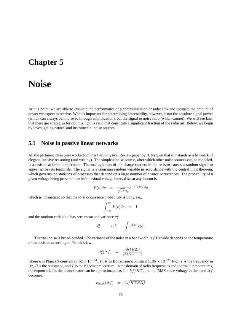
A diagram showing antenna noise temperature versus frequency is shown in Figure 5.3. At frequencies belowabout 15 MHz, antenna noise is dominated by radio emissions from lightning, calledspherics. At HF frequencies,these emissions can propagate from the lightning source (wherever that may be) to the receiver by reflecting from theionosphere. The equivalent noise temperature for these emissions is of the order of1 × 106–1 × 108K.

Between about 15 MHz and 1 GHz, antenna noise is dominated by cosmic radio noise or sky noise. This isemissions from radio stars in our galaxy. The sky noise temperature decreases with frequency at a rate of aboutf−2.4. Cosmic noise at frequencies below 10–15 MHz cannot penetrate the ionosphere. A typical cosmic sky noisetemperature at VHF (UHF) frequencies is about 1000 K (100 K).The actual temperature depends on frequency andalso on direction; cosmic noise is strongest in the direction of the Milky Way center and weakest looking out of theecliptic plane.

81

1 10 1000.10.01Frequency (GHz)

Tem

pera

ture

(k)

104

106

108

102

1

ambient (290 K)

spherics

cosmic noise

galactic center

galactic pole

atmospheric absorption0o

80o

90o wetdry

Figure 5.3: Antenna noise temperature versus frequency.

Cosmic noise continues to decrease with frequency until reaching the 2.7 K background noise temperature atabout 10 GHz. However, antenna noise observed on the ground starts increasing above about 1 GHz due to atmo-spheric absorption noise (see next section). This is radio emission mainly from water vapor in the Earth’s atmosphere.The antenna noise temperature due to atmospheric absorption varies with zenith angle; rays with small zenith an-gles penetrate the atmosphere quickly and so have smaller noise temperatures than rays with low elevations, whichmust traverse a thick atmospheric layer. Atmospheric absorption noise temperatures can be as great as the ambienttemperature, about 200 K.

The radio window refers to the band of frequencies where the terrestrial noise temperature has a minimum. Itis centered in the vicinity of 2 GHz, which is consequently the band where communications links with satellites areconcentrated. The noise temperature here is between 10–100K, depending on time and season, direction, and onatmospheric conditions (relative humidity).

5.2.1 Atmospheric absorption noise and radiative transport

Atmospheric water vapor absorbs radiation from galactic radio sources and also from the sun. While the photosphere(the visible part of the sun) has a temperature of about 6000 K, the corona (the hot plasma surrounding the sun) hasa temperature of 1–2×106 K and is a source of strong background RF radiation. The watervapor blocks some ofthis radiation from reaching the ground but also emits additional noise as a result. The receiver consequently sees acombination of sky noise and atmospheric absorption noise.

What is the connection between atmospheric absorption and noise? To maintain thermodynamic equilibrium,isolated bodies which absorb radiant energy must also radiate. This is just the same principle of detailed balance thatlies at the root of Nyquist’s theorem and the concept of antenna noise temperature. A body absorbing energy increasesin temperature until the energy it radiates matches the energy it absorbs. The terminal temperature may be calculatedusing Planck’s law. We once again do not demand that thermodynamic equilibrium actually exist and can use theradiative transport equations to evaluate noise from atmospheric constituents at any temperature.

We can quantify the effects of atmospheric absorption with the help of Figure 5.4, which depicts a region of the

82

dr

dΩ

L

TSky, Bsky

r=0r=L

Figure 5.4: Diagram illustrating atmospheric absorption noise.

sky to the right being observed through a solid angledΩ by an antenna on the left. In between is a cloud of absorbing(and therefore emitting) material of widthL. The problem is usually described in terms of the noise brightnessBwhich is the noise power density per solid angle,dB = dP/dΩ.

Suppose the brightness in the absence of the cloud is given byBsky . An equation for the differential change inbrightness due to a cloud layer of widthdr is:

dB = −Bαρdr + dBcloud (5.1)

whereα is the absorption cross-section of a cloud molecule andρ is the volume density of the molecules. The firstterm on the right side of (5.1) represents the absorption of noise in the cloud layer, and the second term represents theisotropic emission of noise from the cloud layer due to its thermal energy. Note that the absorption cross-section forwater vapor molecules and droplets depends strongly on dropsize and differs for rain, snow, fog, and humidity. It isalso a strong function of frequency.

Concentrating on the second term for the moment, we can writethe power in watts emitted by the cloud in avolumedv aswρdv, w being the power emitted by each molecule. If the radiation isisotropic, then the associatednoise power density back at the receiver a distancer away and the associated brightness are:

dPcloud =wρdv

4πr2; dv = r2drdΩ

dBcloud = dP/dΩ =wρ

4πdr

All together, the equation for the variation of the brightness from the distant side of the cloud to the near side is givenby

dB

dr+ Bαρ =

wρ

4π(5.2)

This is an elementary ordinary 1st-order differential equation. Before solving it, we can use it to calculate the bright-ness level at which radiative equilibrium is achieved within the cloud. SettingdB/dr = 0 yieldsBcloud = w/4πα.This is the brightness level at which absorption and radiation balance. Greater (lessor) in situ brightness implies netheating (cooling) within the cloud.

Assuming that all the coefficients are constant, the generalsolution to the full differential equation is

B(r) = Be−γr + Bcloud

whereγ = αρ andB is an undetermined coefficient. Note thatr is measured from the far (right) side of the cloudhere. The particular solution comes from enforcing the boundary condition thatB(r = 0) = Bsky . The result is

B = Bskye−γr + Bcloud

(1 − e−γr

)

What is of interest is the brightness at the near (left) side of the cloud, since this is what will be detected by the receiver.Defining theoptical depth of the cloud to beτ ≡ γL gives

B(r = L) = Bskye−τ + Bcloud

(1 − e−τ

)

83

Tant

TlineRx

Tr

Tout

Sin

Figure 5.5: Illustration of the noise budget in a receiving system.

It is noteworthy that, at a given frequency, the same coefficient(γ = αρ) governs the emission and absorption of noisein a medium. This is a consequence of detailed balance and confirms the proposition that good absorbers of radiationare also good radiators. That the solar corona is a strong absorber/emitter at radio frequencies but not in the visiblespectrum is a vivid example of how these properties can depend strongly on frequency, however.

Finally, by applying Nyquist’s theorem, we can quantify thenoise equally well by an equivalent noise temperatures:

Tant = Tskye−τ + Tcloud

(1 − e−τ

)(5.3)

All together, atmospheric absorption is quantified by the optical depth of the absorbing medium. Large (small) valuesof τ denote an opaque (transparent) atmosphere. To a ground-based observer, atmospheric absorption decreases thedirect radiance of the sun. However, the observer will also see RF radiation from the atmosphere itself, which is beingheated by absorption and which must radiate in pursuit of thermal equilibrium. The antenna noise temperature con-sequently equals the sky noise temperature given a perfectly transparent atmosphere but the atmospheric temperature(calledTcloud here) for a perfectly opaque one. Note that whereasTsky can depend strongly on frequency,Tcloud isthe actual atmospheric temperature at cloud level (∼200-300 K) and does not vary greatly with frequency, althoughthe optical depth does.

The idea presented above can be applied to other situations.For example, radio receivers on spacecraft sometimesstare down at the Earth rather than up into space. In this case, the background noise source is the Earth itself, whichradiates with the noise temperature of the ground. Equation(5.3) still applies, only withTsky replaced byTground. Notonly can atmospheric water vapor and other constituents be observed from variations in the antenna noise temperature,so can other features that effect emission and absorption. These include ground cover, forest canopies, and features inthe terrain.

5.2.2 Feedline absorption

We can extend the ideas from the previous section to a treatment of non-ideal, absorbing transmission lines. Thesetoo must radiate (emit noise) if thermodynamic equilibriumis to be maintained, and the noise they contribute can bemodeled according to (5.3).

As shown in Figure 5.5, there are actually three sources thatcontribute to the output noise of a receiver. Theseare the antenna (with contributions from spherics, cosmic sky noise, and/or atmospheric absorption), the transmissionline, and the receiver itself. The last of these will be analyzed in the next section. For now, it is sufficient to saythat each of these noise sources can be characterized by an equivalent noise temperature, and that the receiver noisetemperatureTr is additive. We have already discussedTant. The noise temperature for the transmission lineTline

(which we assume to be the ambient temperature,∼300 K) is incorporated just as in (5.3)

Tout = Tante−γL + Tline

(1 − e−γL

)+ Tr

Here,γ is the transmission line attenuation constant per unit length, L is the line length, andγL is the equivalentoptical depth for the line. A common shorthand is to write theexponential term as a single factorǫ, representing thefraction of the input power that exits the line, i.e.

Tout = Tantǫ + Tline (1 − ǫ) + Tr

84

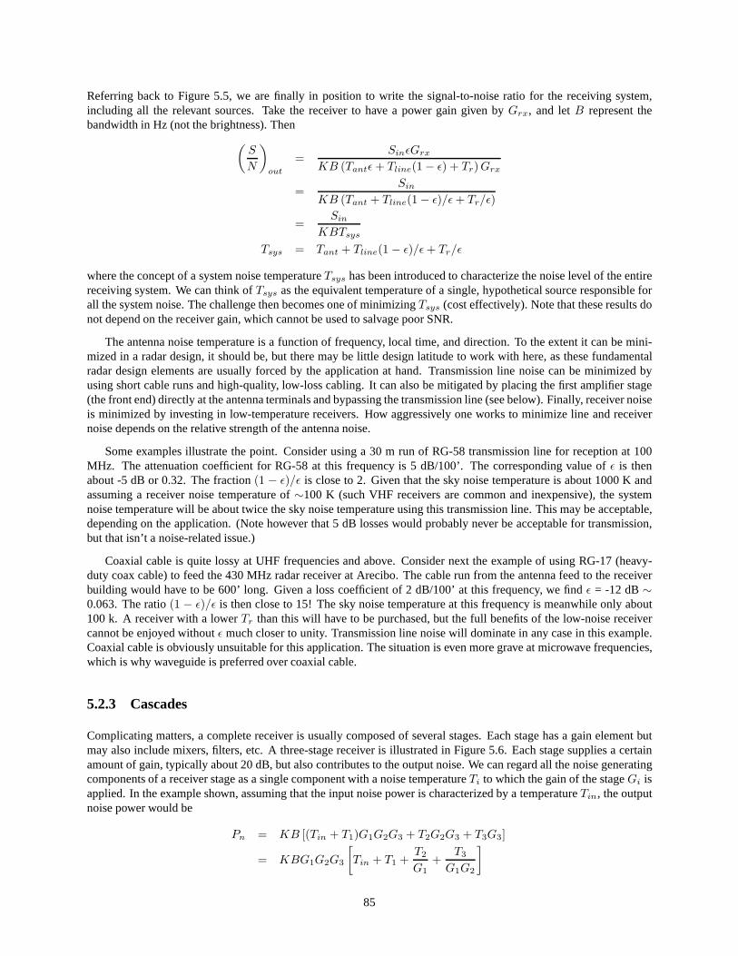
Referring back to Figure 5.5, we are finally in position to write the signal-to-noise ratio for the receiving system,including all the relevant sources. Take the receiver to have a power gain given byGrx, and letB represent thebandwidth in Hz (not the brightness). Then

(S

N

)

out

=SinǫGrx

KB (Tantǫ + Tline(1 − ǫ) + Tr)Grx

=Sin

KB (Tant + Tline(1 − ǫ)/ǫ + Tr/ǫ)

=Sin

KBTsys

Tsys = Tant + Tline(1 − ǫ)/ǫ + Tr/ǫ

where the concept of a system noise temperatureTsys has been introduced to characterize the noise level of the entirereceiving system. We can think ofTsys as the equivalent temperature of a single, hypothetical source responsible forall the system noise. The challenge then becomes one of minimizing Tsys (cost effectively). Note that these results donot depend on the receiver gain, which cannot be used to salvage poor SNR.

The antenna noise temperature is a function of frequency, local time, and direction. To the extent it can be mini-mized in a radar design, it should be, but there may be little design latitude to work with here, as these fundamentalradar design elements are usually forced by the applicationat hand. Transmission line noise can be minimized byusing short cable runs and high-quality, low-loss cabling.It can also be mitigated by placing the first amplifier stage(the front end) directly at the antenna terminals and bypassing the transmission line (see below). Finally, receiver noiseis minimized by investing in low-temperature receivers. How aggressively one works to minimize line and receivernoise depends on the relative strength of the antenna noise.

Some examples illustrate the point. Consider using a 30 m runof RG-58 transmission line for reception at 100MHz. The attenuation coefficient for RG-58 at this frequencyis 5 dB/100’. The corresponding value ofǫ is thenabout -5 dB or 0.32. The fraction(1 − ǫ)/ǫ is close to 2. Given that the sky noise temperature is about 1000 K andassuming a receiver noise temperature of∼100 K (such VHF receivers are common and inexpensive), the systemnoise temperature will be about twice the sky noise temperature using this transmission line. This may be acceptable,depending on the application. (Note however that 5 dB losseswould probably never be acceptable for transmission,but that isn’t a noise-related issue.)

Coaxial cable is quite lossy at UHF frequencies and above. Consider next the example of using RG-17 (heavy-duty coax cable) to feed the 430 MHz radar receiver at Arecibo. The cable run from the antenna feed to the receiverbuilding would have to be 600’ long. Given a loss coefficient of 2 dB/100’ at this frequency, we findǫ = -12 dB∼0.063. The ratio(1 − ǫ)/ǫ is then close to 15! The sky noise temperature at this frequency is meanwhile only about100 k. A receiver with a lowerTr than this will have to be purchased, but the full benefits of the low-noise receivercannot be enjoyed withoutǫ much closer to unity. Transmission line noise will dominatein any case in this example.Coaxial cable is obviously unsuitable for this application. The situation is even more grave at microwave frequencies,which is why waveguide is preferred over coaxial cable.

5.2.3 Cascades

Complicating matters, a complete receiver is usually composed of several stages. Each stage has a gain element butmay also include mixers, filters, etc. A three-stage receiver is illustrated in Figure 5.6. Each stage supplies a certainamount of gain, typically about 20 dB, but also contributes to the output noise. We can regard all the noise generatingcomponents of a receiver stage as a single component with a noise temperatureTi to which the gain of the stageGi isapplied. In the example shown, assuming that the input noisepower is characterized by a temperatureTin, the outputnoise power would be

Pn = KB [(Tin + T1)G1G2G3 + T2G2G3 + T3G3]

= KBG1G2G3

[

Tin + T1 +T2

G1+

T3

G1G2

]

85

T1 G1 T2 G2 T3 G3Sin +KT inB

output

RF

LO

IFfilter

ω0

ωm

ω0±ωm ω0−ωm

Tin=Tantε + ΤL(1−ε)

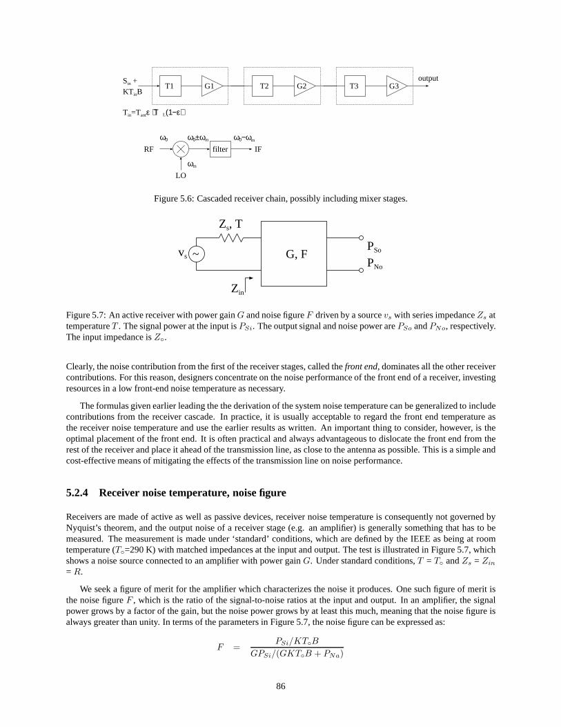
Figure 5.6: Cascaded receiver chain, possibly including mixer stages.

~vs

Zs, T

G, F

Zin

PSo

PNo

Figure 5.7: An active receiver with power gainG and noise figureF driven by a sourcevs with series impedanceZs attemperatureT . The signal power at the input isPSi. The output signal and noise power arePSo andPNo, respectively.The input impedance isZ.

Clearly, the noise contribution from the first of the receiver stages, called thefront end, dominates all the other receivercontributions. For this reason, designers concentrate on the noise performance of the front end of a receiver, investingresources in a low front-end noise temperature as necessary.

The formulas given earlier leading the the derivation of thesystem noise temperature can be generalized to includecontributions from the receiver cascade. In practice, it isusually acceptable to regard the front end temperature asthe receiver noise temperature and use the earlier results as written. An important thing to consider, however, is theoptimal placement of the front end. It is often practical andalways advantageous to dislocate the front end from therest of the receiver and place it ahead of the transmission line, as close to the antenna as possible. This is a simple andcost-effective means of mitigating the effects of the transmission line on noise performance.

5.2.4 Receiver noise temperature, noise figure

Receivers are made of active as well as passive devices, receiver noise temperature is consequently not governed byNyquist’s theorem, and the output noise of a receiver stage (e.g. an amplifier) is generally something that has to bemeasured. The measurement is made under ‘standard’ conditions, which are defined by the IEEE as being at roomtemperature (T=290 K) with matched impedances at the input and output. The test is illustrated in Figure 5.7, whichshows a noise source connected to an amplifier with power gainG. Under standard conditions,T = T andZs = Zin

= R.

We seek a figure of merit for the amplifier which characterizesthe noise it produces. One such figure of merit isthe noise figureF , which is the ratio of the signal-to-noise ratios at the input and output. In an amplifier, the signalpower grows by a factor of the gain, but the noise power grows by at least this much, meaning that the noise figure isalways greater than unity. In terms of the parameters in Figure 5.7, the noise figure can be expressed as:

F =PSi/KTB

GPSi/(GKTB + PNa)

86

= 1 +PNa

GKTB

wherePNa is the noise power produced within the amplifier itself. Withsome rearranging, we can find thatPNa =G(F −1)KTB. This is the noise power that would be produced by the input resistor if it were raised to a temperatureTf = (F − 1)T. This temperature is called the amplifier noise temperature. It typically does not correspond to theactual temperature of the device, although the two may be related.

Noise temperature is one figure of merit of a receiver, and noise figure is another. The two metrics are reallyequivalent; manufacturers tend to quote the former when thenoise temperature is less than ambient (300 K) andthe latter otherwise. Noise figures are often quoted in dB. For example, a receiver with a very respectable noisetemperature of 30 K has a noise figure of about 0.4 dB. Such a receiver would probably be cryogenically cooled.

Under nonstandard conditions, the actual noise performance of the amplifier will deviate from what is describedabove. Referring back to Figure 5.7, consider what happens when the input noise source temperature, source impedance,and input impedance are allowed to assume arbitrary values.In this case, the input noise power must be written as

PNi = KTB4Rs

|Zs + Zin|2Rin ≡ MKTB

where Nyquist’s theorem has been invoked,KTB is the available noise power, andM is therefore the impedancemismatch factor. The output noise power is consequently

PNo = GMKTB + PNa = GKTB(M + (F − 1)T/T )

The signal input power is

PSi =

∣∣∣∣

vs

Zs + Zin

∣∣∣∣

2

Rin =|vs|24Rs

M

and the output signal power is justG times this. The output signal to noise ratio can then be expressed as:

PSo

PNo=

|vs|24RsKTB

M

M + (f − 1)T/T

Finally, we can calculate the ratio of the input to output signal-to-noise ratio. Note that this is not the noise figure,which is defined for standard conditions, but is instead the effective noise figureF ′:

F ′ = 1 +(F − 1)T/T

M

Under matched conditions, this reverts to the usual noise figure as it must. Improper impedance matching introducesa value ofM less than unity and implies degraded noise performance. A value ofT that is greater thanT meanwhileimplies strong input noise, making the effects of amplifier noise less significant and reducing the effective noise figure.

5.2.5 Receiver bandwidth

Noise power is proportional to bandwidth, and in the contextof radar receivers, it is the receiver bandwidth that is inquestion. Decreasing the bandwidth decreases the noise at the cost of possibly decreasing the information available inthe received signal. In the case of signals with binary encoded information, the bandwidth is proportional to the bitrate. In radar applications, the bandwidth of the received signals is related to the reciprocal of the radar pulse width.A 1µs pulse has a bandwidth of about 1 MHz. Narrower radar pulses permit measurements of increasingly fine detailsin the targets at the expense of increased noise power.

5.3 Matched filters

Perhaps the most critical component in a receiver is the filter which determines which parts of the received signal andnoise are passed along for processing. Most often (but not always), filters are designed to maximize the signal to noise

87

ratio at their output. The matched filter theorem discussed below provides a recipe for accomplishing this. “Matched”in this case refers not to an impedance or polarization match(both of which are also important) but to an optimalmatch between the filter characteristics and the signals likely to be encountered.

We consider a linear filter with inputx(t) = f(t) + n(t) and outputy(t) = yf (t) + yn(t), wheref andn refer tothe signal and noise components, respectively. The objective is to optimize the filter spectrumH(ω) or equivalentlythe impulse response functionh(t) to maximize the output signal to noise power ratio at some timet. Note thatH(ω)andh(t) are a Fourier transform pair,H(ω) =

∫f(t) exp(−jωt)dt = F(f(t)). The output signal power is just the

square modulus ofyf (t). Noise is a random variable, and the noise power is the expectation of the square modulus ofyn(t). Therefore, we maximize the ratioR:

R =|yf (t)|2

E(|yn(t)|2)While we do not have access to the expectation of the noise power, we can assume the noise to be statistically stationaryand approximate the expectation with a time average〈〉.

Let F (ω) andN(ω) be the frequency-space representations of the input signaland noise, respectively. We candefine the signal and noise as being nonzero over only a finite span of timeT to avoid problems associated with thedefinitions ofF (ω) andN(ω), which involve integrals over all times (see chapter 1). Theunits of these two quantitiesare the units ofy(t) per Hz. Still in the frequency domain, the output signal and noise are the productsF (ω)H(ω) andN(ω)H(ω). In the time domain, the output noise is then

yn(t) = F−1(N(ω)H(ω))

=1

2π

∫

N(ω)H(ω)ejωtdω

At any instant in time, the output noise power is

yn(t)y∗

n(t) =

(1

2π

)2 ∫

N(ω)H(ω)ejωtdω

∫

N∗(ω′)H∗(ω′)e−jω′tdω′

The time average of the power over the intervalT is

〈yn(t)y∗

n(t)〉 =1

T

(1

2π

)2 ∫ ∫ ∫

N(ω)N∗(ω′)H(ω)H∗(ω′) ej(w−w′)tdt︸ ︷︷ ︸

2πδ(ω−ω′)

dωdω′

=1

T

1

2π

∫

|N(ω)|2|H(ω)|2dω

=1

2π

∫

Sn(ω)|H(ω)|2dω

whereSn(ω) is the power spectrum of the noise with units of power per Hz. The noise usually has a nearly flatspectrum over the bandwidth of interest (white noise), and so this is just a constantS.

Incorporating these results in the signal-to-noise ratio expression gives

R|t =| 12π

∫F (ω)H(ω)ejωt |2

S

2π

∫|H(ω)|2dω

(5.4)

We are not interested in evaluating (5.4) but rather on conditioning its upper limit. This can be done with the help oftheSchwartz inequality

∣∣∣∣∣

∫ b

a

f(x)g(x)dx

∣∣∣∣∣

2

≤∫ b

a

|f(x)|2dx

∫ b

a

|g(x)|2dx (5.5)

Identifyingf = F , andg = Hejωt such that|g|2 = |H |2 reveals the relevance to (5.4). The maximum signal to noiseratio is consequently achieved when the equality above is satisfied. This obviously occurs whenf∗ = g, or in our casewhen

H(ω)ejωt = F ∗(ω)

88

t0 t0t t

f(t) h(t)=f*(t0-t)

t0t

yf(t)=∫t−∞f(t’)f *(t-t’)dt’

h(t)f(t) yf(t)

t0t’

f(t’)

tt-t0

f(t0-t+t’)

Figure 5.8: Matched filter detection of an anticipated signal. The filter is optimized for sampling at timet, which isset here to coincide with the trailing end off(t).

which is the matched filter theorem. The meaning is clearer inthe time domain:

H(ω) = AF ∗(ω)e−jωt

h(t) =1

2π

∫

AF ∗(ω)e−jωtejωtdω

=1

2π

∫

AF ∗(ω)ejω(t−t)dω

=

[1

2π

∫

AF (ω)ejω(t−t)dω

]∗

= Af∗(t − t)

which is to say that the impulse response function of the optimal filter is proportional to the complex conjugate of thetime reverse of the anticipated signal.

Figure 5.8 shows an anticipated signalf(t) (the reflection of a transmitted radar pulse, for example) and the optimalfilter impulse response function for detection at timet, which is set here to coincide with the trailing edge off(t).Noise has been neglected for the moment. By selectingt this way, the filter impulse response function will always“turn on” at t = 0, which will be convenient for implementation. The filter output is the convolution of the input andthe impulse response function, a kind of integral over past history.

yf (t) =

∫ t

−∞

f(t′)h(t − t′)dt′

where the impulse response function determines how much of the past to incorporate. Using a matched filter,

h(t − t′) = f∗(t − (t − t′))

yf (t) =

∫

f(t′)f∗(t − t + t′)dt′

This integral is the inner product of a function with itself or its autocorrelation function. The convolution operatoris therefore made to be the correlation of the input (signal plus noise) with a delayed copy of the anticipated signal.

89

τ T T+τ T+2τ

R

Tx Rx

Tx

f(t)

h(t)

f ⊗ h

t0

t

t

t

t

Figure 5.9: Radar experiment using a square pulse.

The former (latter) will be well (poorly) correlated, and the signal-to-noise ratio will be maximized at the timet = t.Note thatyf (t) is related to the total energy in thef(t) waveform.

The impulse response function is so named because it gives the response of the filter to an impulse

yδ(t) =

∫

δ(t′)h(t − t′)dt′

= h(t)

In the laboratory, this can be measured either by applying animpulse at the input and monitoring the output on anoscilloscope or by applying white noise at the input and viewing the output with a spectrum analyzer. Analog filterscan be designed to replicate many desirable functions approximately. Digital filters can be much more precise.

5.4 Two simple radar experiments

All of this material can be placed in context with the consideration of a some simple radar experiments. The firstis illustrated in Figure 5.9, which depicts the transmission and reception of a square radar pulse (widthτ ) which isscattered or reflected from a mirror target, so that the received signal is a time-delayed copy of the transmitted pulse.The delay time isT = 2R/c, the travel time out and back.

Figure 5.9 also shows the impulse response functionh(t) = f(t − t) (we takef to be real here). This is justthe time reverse of the original pulse, which remains rectangular. By takingt = T + τ , the time corresponding tothe trailing edge off(t), we demand the matched filter impulse response function to turn on att = 0. In fact, thereasoning goes the other way around: we will always by convention designh(t) so that it turns on att = 0, meaningthat the filter output will always be a maximum at the trailingedge off(t) no matter what the shape or delay of thatfunction. This will ultimately allow us to estimate the travel timeT of an echo from the peak in the filter output.

Finally, the figure shows the convolution of the received signal with the impulse response function. This is thefilter output, essentially the correlation of the transmitted waveform with a delayed replica of itself. It spans the timeinterval fromT to T + 2τ and has a half widthτ . The output is greatest att = t = T + τ , as it was designed to be.The shape is triangular, but the output power (which is proportional to the square of the output voltage) is more sharplypeaked. Note that the apparent range of the target isR + cτ/2 here and that the extra delayτ has to be consideredwhen assigning radar range to an echo. Of course, we do not generally knowT a priori but rather seek to determine itfrom peaks in the output. The filter is usually sampled continuously or at least over a broad span of times (the sampleraster), and potential targets are identified from peaks in the output.

90

t

t

t

h(t)

xmit

output

2R/c+3τ

τ

τ

t

f(t)

2R/c

t0

Figure 5.10: Radar experiment using a 3-bit coded square pulse.

The radar pulse width determines the bandwidth of the matched filter, which determines the noise level and ulti-mately limits detectability. The pulse width also determines the range resolution of the experiment, or the ability todiscern echoes closely spaced in range. In this example, therange resolution is roughly the half width of the filter, orroughly the pulse length. Echoes spaced more closely thanδr = cτ/2 would be difficult to distinguish. Finally, thepulse width determines (or is limited by) the duty cycle of the pulsed radar. The fraction of the time that high-powertransmitters can be in the ‘on’ state varies from about 2–20%depending on their design. Compared to vacuum tubetransmitter amplifiers, solid-state amplifiers tend to operate at lower peak power levels but with higher maximum dutycycles.

The same reasoning can be applied to the analysis of a slightly more complicated radar experiment. Figure 5.10shows an experiment in which the transmitted waveform is phase modulated (0 or 180) so as to form the numericalcode 1, 1, -1. The bit width isτ , and the pulse width is 3τ . Such binary coded sequences are readily generated usingsimple RF switching networks or through digital synthesis.The corresponding impulse response functionh(t) formatched filtering is also shown. Once again, the convention is to design the matched filter to have an impulse responsefunction that starts att = 0. This makes the time for maximum filter outputt = T + 3τ coincide with the trailingedge of the inputf(t) no matter what the shape or range delay of that function.

The convolution of the received signal and the impulse response function gives the filter output for an echo froma single mirror target. Compared to the uncoded pulse example where the pulse width was justτ , we find that theamplitude of the filter output has grown by a factor of 3. The half width of the main response, however, has not grownand remains roughlyτ . Some range sidelobes, which will be detrimental to detection, have also appeared, however.While there is no noise explicitly in this problem, we can show that the noise level for the coded pulse experimentwould be greater than that for the uncoded pulse by a factor of

√3. Consequently, the signal-to-noise power ratio grew

by a factor of 3. Another way to think about signal-to-noise improvement in pulse coding is this: since the coded pulsecontains three times the energy of an uncoded pulse of lengthτ but has roughly the same bandwidth, we should expecta signal-to-noise ratio improvement of a factor of 3.

91

vin

vout

∆v

Figure 5.11: Quantization noise.

By using the same filter to process all possible echo signals (one with anh(t) that begins att = 0), we get amaximum response at a delay time related to the delay off(t) and the range of the target. Note however that themaximum filter output occurs at a delay timet = 2R/c + 3τ in this example. As in the previous example, the lengthof the pulse must be taken into account when associating the filtered echo delay with the range of the target.

Pulse coding provides a means of increasing the duty cycle ofa radar experiment and the signal-to-noise ratiowithout degrading range resolution. A downside of pulse coding is the introduction ofclutter or echoes from rangesother than the “correct” one. We will study and evaluate various pulse coding schemes in chapter 8. What we haveseen already hints about how radar waveforms can be optimized to achieve different objectives.

5.5 Quantization noise

Another kind of noise unrelated to nature and Nyquist’s theorem usually turns up in radar experiments. This is noiseassociated with the quantization (digitization) of an analog signal. As depicted in Figure 5.11, quantization causessmall, pseudo-random discrepancies between the analog anddigital representation of a signal, and these discrepanciesconstitute noise. Quantization noise is often but not always negligible and depends on the quantization resolution∆v.

The largest error associated with quantization is±∆v/2. Let us treat the instantaneous error as a zero meanrandom variableδv uniformly distributed on the interval[±∆v/2]. The associated noise power is proportional to thenoise variance

〈δv2〉 =1

∆v

∫ ∆v/2

−∆v/2

δv2dδv

=1

12

(∆v2

)

Is this significant compared to background noise power? Suppose we use an 8-bit digitizer (256 levels) and setthe receiver gain so that the background noise level has an RMS voltage level of 10∆v. In that case, the ratio ofquantization noise to background noise is given by

Nq

N=

1/12

102= −31 dB

Quantization noise is therefore not very significant. Next consider what happens if the receiver gain is set so that the

92

background noise toggles just one bit of the digitizer.

Nq

N=

1/12

1= −11 dB

This is still small, but perhaps not negligible. The real danger occurs when the background noise fails to toggle reliablyeven one bit of the digitizer. In that case, quantization noise may dominate, leading to significant degradation of theoverall signal-to-noise ratio. It is best to set the receiver gain so that at least a few bits are continuously toggled bybackground noise. It may be difficult to do this while simultaneously avoiding saturation by strong signals. If so, adigitizer with finer precision (more bits) may be necessary.Even a saturated signal contains a surprising amount ofinformation, however; one-bit digitization was once used extensively before high-speed wide-word digitizers becameavailable.

5.6 References

5.7 Problems

93

Chapter 6

Scattering

We now know enough about radar hardware analysis and design to begin to address the objective of radar, which isto derive meaningful information from radio signals scattered by distant targets. What is the nature of the scattering,and how do we quantify it? The scattering cross section is a parameter which describes the power scattered by anobject exposed to electromagnetic radiation. For some objects, it can be calculated from first principles (electrons,rain drops). For others (aircraft, ships), it usually must be measured. Sometimes, it is simply related to the physicalsize of the object. Sometimes, it is not. It generally depends on the radar frequency, polarization, and orientation.Some definitions help clarify the distinctions.

Referring to the schematic diagram in Figure 6.1, we can express the power density incident on the target in termsof the transmitted powerPtx, the range to the targetr, and the antenna gainG as

Pinc =PtG

4πr2(W/m)

Define thetotal scattering cross section σt as the total power scattered per incident power density, or

Psc = Pincσt

Scattering is a kind of radiation, and the scattering can no more be isotropic than the initial radiation. Therefore, definethe scattering directivityDs as the ratio of the scattered power density back at the receiver to the power density thatwould exist if the scattering were isotropic. Then the received power will be

Prx =DsPsc

4πr2Aeff

=PtxG

4πr2σtDs

Aeff

4πr2

where the antenna gain and effective area are related by the reciprocity theorem if the same antenna is used for transmitand receive as in Figure 6.1. Finally, the total scattering cross section and scattering directivity are often combinedinto a single parameter, theradar scattering cross section σ = σtDs. This is defined as the total scattered power per

target shadow

G

Tx

Rx

Figure 6.1: Radar illuminating a target.

94

incident power density that, if scattered isotropically, would give rise to the observed power back at the receiver. Thisis a useful engineering definition.

Finally, assuming no impedance or polarization mismatches, the entire power budget can be represented by theradar equation:

Prx

Ptx=

G2λ2σ

(4π)3r4

which applies to scatter from lone, “hard” targets. Note that the ratio above does not actually scale asλ2; both the gainand the radar cross section include additional wavelength dependence.

Confusion surrounds the definitions ofσt andσ, and it is worth reemphasizing their differences. The former is theeffective aperture of the scatterer which collects incident power and scatters it away from the original direction. Thisconcept is useful for studying signal attenuation along itspropagation path, for example. The latter is the effectivearea which, if scattering power isotropically, would result in the power actually observed back at the radar. This isusually what concerns radar specialists. A third definitionsometimes used is the geometric or physical scattering crosssection,Ag = Ap ∼ πa2, wherea is something like the scatterer dimension. This is the shadow area cast by thetarget. We can also define the backscatter efficiency as the ratio of the radar scattering cross section to the physicalcross section,ǫs ≡ σ/Ag.

The scattering cross section may depend on

1. target size and shape

2. target material

3. frequency

4. polarization

5. target orientation

We investigate these dependencies below.

6.1 Rayleigh scatter

There are three scattering regimes of interest: theRayleigh regime (a ≪ λ), optical regime (a ≫ λ), and theresonanceregime (a ∼ λ). In the Rayleigh regime, the scatterer is small compared toa wavelength, and at any given time,the electric field supplied by the radar is spatially uniformthroughout the scatterer volume. What happens next isillustrated in Figure 6.2. While a spherical target is considered to simplify the calculations, the shape of the target doesnot affect the backscatter in the Rayleigh regime.

When exposed to a uniform background electric field, chargeswithin the target (a spherical dielectric) rearrangethemselves so as to minimize their configurational energy. The final configuration is an electric dipole. As indicatedin the figure, the electric field within the target remains uniform but is reduced. Outside, the electric field is thebackground field plus the field of an ideal electric dipole. Asthe phase of the wave changes over time with angularfrequencyω, so does the polarity of the induced electric dipole. Associated with the constant rearrangement of chargeis an elemental current (see derivation in appendix)

Idl = jω4πa3 ǫ − ǫǫ + 2ǫ

ǫE

whereǫ is the permittivity of the dielectric sphere. What has therefore been created is an ideal electric dipole antenna.We already have expressions for calculating the incident power density associated withE and the total power radiated

95

a--

-+

+

+

E0

λ

Figure 6.2: Rayleigh scatter from a spherical target of radiusa. The illuminating signal propagates vertically and ispolarized in the plane of the figure.

associated withIdl. The ratio gives the total scattering cross sectionσt for the target.

σt =128

3

(πa2

)π4

(ǫ − ǫǫ + 2ǫ

)2 (a

λ

)4

In the event the scatterer is a conductor rather than a dielectric, the term involving the ratio of the permittivities shouldbe replaced by unity. Finally, the radar scattering cross section can be calculated by multiplyingσt by the directivity,which we know to be 1.5 for backscatter from an elemental dipole antenna. Taking the ratio of the radar scatteringcross section to the physical area of the target gives the backscatter efficiency

ǫs ∝(

2πa

λ

)4

= C4λ

which gives the Rayleigh scattering result, that the backscatter efficiency is proportional to the target circumference(in wavelengths) to the fourth power. This result explains,among other things, why the sun appears red and the skyblue to a terrestrial observer.

6.2 Mie scatter

Scattering from dielectric and conducting spheres that arenot physically small compared to a wavelength is calledMie scatter and is illustrated on the right side of the graph in Figure 6.3. In this situation, the polarity of the electricfield is different at different scattering depths, and so therefore is the induced polarization. Destructive or constructiveinterference occurs between the backscatter signal components from different depths. The backscatter efficiencyoscillates around a value of unity for different values ofCλ. Large atmospheric aerosols are responsible for Miescattering of light, which we see in smog.

6.3 Specular reflection

The Mie scattering behavior in Figure 6.3 applies only to scatterers that are roughly spherical. Scattering efficiencyin the optical regime is a strong function of the shape and orientation of the scatterer. Much more efficient than Miescatter is backscattering from roughly flat surfaces, whichwe refer to here as specular reflection or scatter (i.e. as

96

0.1 1 10

100

10

1

.1

.01

Cλ

εs

C2λ

C4λ

Rayleighscatter

Miescatter

specularreflection

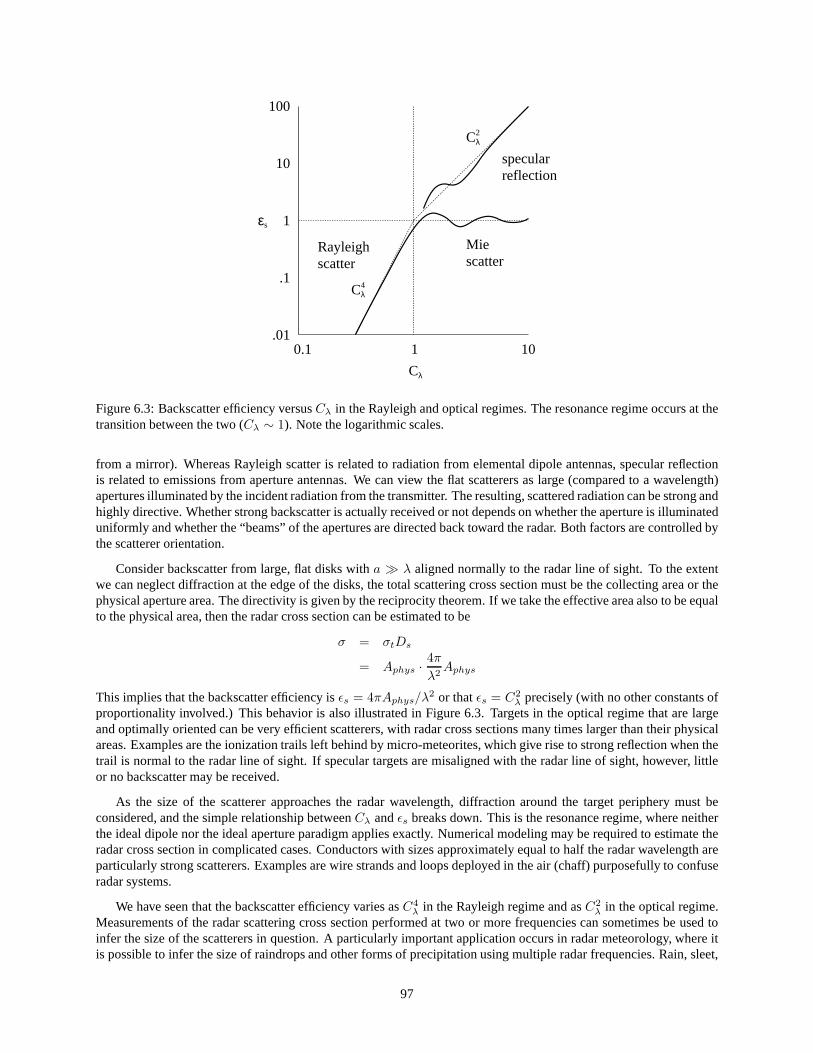
Figure 6.3: Backscatter efficiency versusCλ in the Rayleigh and optical regimes. The resonance regime occurs at thetransition between the two (Cλ ∼ 1). Note the logarithmic scales.

from a mirror). Whereas Rayleigh scatter is related to radiation from elemental dipole antennas, specular reflectionis related to emissions from aperture antennas. We can view the flat scatterers as large (compared to a wavelength)apertures illuminated by the incident radiation from the transmitter. The resulting, scattered radiation can be strong andhighly directive. Whether strong backscatter is actually received or not depends on whether the aperture is illuminateduniformly and whether the “beams” of the apertures are directed back toward the radar. Both factors are controlled bythe scatterer orientation.

Consider backscatter from large, flat disks witha ≫ λ aligned normally to the radar line of sight. To the extentwe can neglect diffraction at the edge of the disks, the totalscattering cross section must be the collecting area or thephysical aperture area. The directivity is given by the reciprocity theorem. If we take the effective area also to be equalto the physical area, then the radar cross section can be estimated to be

σ = σtDs

= Aphys ·4π

λ2Aphys

This implies that the backscatter efficiency isǫs = 4πAphys/λ2 or thatǫs = C2λ precisely (with no other constants of

proportionality involved.) This behavior is also illustrated in Figure 6.3. Targets in the optical regime that are largeand optimally oriented can be very efficient scatterers, with radar cross sections many times larger than their physicalareas. Examples are the ionization trails left behind by micro-meteorites, which give rise to strong reflection when thetrail is normal to the radar line of sight. If specular targets are misaligned with the radar line of sight, however, littleor no backscatter may be received.

As the size of the scatterer approaches the radar wavelength, diffraction around the target periphery must beconsidered, and the simple relationship betweenCλ andǫs breaks down. This is the resonance regime, where neitherthe ideal dipole nor the ideal aperture paradigm applies exactly. Numerical modeling may be required to estimate theradar cross section in complicated cases. Conductors with sizes approximately equal to half the radar wavelength areparticularly strong scatterers. Examples are wire strandsand loops deployed in the air (chaff) purposefully to confuseradar systems.

We have seen that the backscatter efficiency varies asC4λ in the Rayleigh regime and asC2

λ in the optical regime.Measurements of the radar scattering cross section performed at two or more frequencies can sometimes be used toinfer the size of the scatterers in question. A particularlyimportant application occurs in radar meteorology, where itis possible to infer the size of raindrops and other forms of precipitation using multiple radar frequencies. Rain, sleet,

97

r

r2dΩ

∆r=cτ/2

Figure 6.4: Geometry of a radar scattering volume.

hail, and snow come in recognizable sizes, and it is therefore possible to identify precipitation types from scatterersize. Rainfall rates can also be calculated from simultaneous drop size and fall velocity estimates.

A few other types of radio scatter have roles to play in different radar applications. These include

• Bragg scatter, which occurs from rough surfaces. Sea surface backscatter is an important example that allowsremote sensing of ocean currents.

• Thomson scatter, which occurs when free electrons are caused to oscillate by incident RF radiation. A modifiedform of Thomson scatter permits the measurement of certain plasma parameters in the Earth’s ionosphere.

• Reflection from corner reflectors, which makes certain man-made objects in particular easy to detect with radar.

• Total reflection, as occurs for HF radiation propagating into the Earth’s ionosphere.

• Partial reflection from gradients in the index of refraction. Ground penetrating radars (GPR) use this phe-nomenon to explore geological and archaeological featuresburied beneath the Earth’s surface.

6.4 Volume scatter

The preceding discussion dealt with radar backscatter froma single target. Frequently, multiple targets reside withinthe radarscattering volume. This is the volume defined in three dimensions by the beam solid angle, the range, andthe radar pulse width/ matched filter width (see Figure 6.4).The cross-sectional area of the volume isr2dΩ, and thedepth of the volume iscτ/2, whereτ is the pulse width to which the receiver filter is presumably matched (see nextchapter).

The targets in question could be electrons, raindrops, or insects; in the discussion that follows, they are assumedto be identical and randomly distributed throughout the volume. We further assume that the targets are insufficientlydense to cause significant attenuation of the radar signal passing through the volume. This is referred to as theBornlimit. In this limit, we can define a radar scattering cross sectionper unit volumeσv as the product of the radar crosssection for each target times the number density of targets per unit volume,σv = Nσ.

The power density incident on the scattering volume is

Pinc = PtxG(θ, φ)

4πr2

whereG is the gain and wherer, θ, andφ are measured from the antenna. The differential power scattered by eachsub volumeδV within the scattering volume is then given by

dPs = PincσvdV

In view of the definition of the radar scattering cross section, the corresponding amount of power received fromscattering withindV will be

dPrx = PincσvAeff (θ, φ)

4πr2dV

98

Now, takingdV = ∆rr2dΩ = (cτ/2)r2 sin θdθdφ and integrating over the entire scattering volume for this rangegate gives

Prx =

∫

PtxG(θ, φ)

4πr2σv

Aeff (θ, φ)

4πr2

cτ

2r2 sin θdθdφ

=Ptxσvcτλ2

32π2r2

1

4π

∫ 2π

0

dφ

∫ π

0

dθ G2(θ, φ) sin θ

︸ ︷︷ ︸

Gbs

where the reciprocity theorem has been invoked and where thebackscatter gain and corresponding backscatter area ofthe antenna have been defined:

Gbs =1

4π

∫ 2π

0

dφ

∫ π

0

dθ G2(θ, φ) sin θ

≡ 4π

λ2Abs

These are new quantities, not to be confused with the standard antenna gain and effective area. They are constantsrather than functions which quantify signal returns in volume scatter situations. They account for the fact that theantenna gain determines not just the power received from an individual scatterer but also the size of the scatteringvolume and therefore the number of scatterers involved. It is always true that the backscatter gain is less than themaximum gain and the backscatter area is less than the physical area of the antenna, typically by a factor of about onehalf.

All together, the received power as a fraction of the transmitted power is

Prx

Ptx=

σvcτλ2

32π2r2Gbs

=σv

4πr2

cτ

2Abs (6.1)

∝ Abs

r2

Contrast this with the behavior for single (hard target) backscatter, where the ratio is proportional to(Aeff/r2)2.Since the noise power given by Nyquist’s theorem is proportional to the bandwidth which is the reciprocal of the pulsewidth, we may further write

S

N=

Ptxσv

2π

(∆r

r

)2Abs

KbTc

∝(

∆r

r

)2

where we make use of∆r = cτ/2. This expression exemplifies the high cost of fine range resolution in volumescattering situations. In the next two chapters, we will explore how to optimize radar experiments and signal processingin order to deal with weak signals. Pulse compression in particular will be seen to be able to recover one factor of∆r.

6.5 References

6.6 Problems

99