Embed Size (px)
Citation preview
ANSI/ASHRAE Addendum a toANSI/ASHRAE Standard 140-2011
Standard Method of Testfor the Evaluation of
Building Energy AnalysisComputer Programs
Approved by the ASHRAE Standards Committee on June 28, 2014; by the ASHRAE Board of Directors on July 2, 2014; and by theAmerican National Standards Institute on July 3, 2014.
This addendum was approved by a Standing Standard Project Committee (SSPC) for which the Standards Committee has estab-lished a documented program for regular publication of addenda or revisions, including procedures for timely, documented, con-sensus action on requests for change to any part of the standard. The change submittal form, instructions, and deadlines may beobtained in electronic form from the ASHRAE website (www.ashrae.org) or in paper form from the Manager of Standards.
The latest edition of an ASHRAE Standard may be purchased on the ASHRAE website (www.ashrae.org) or from ASHRAE Cus-tomer Service, 1791 Tullie Circle, NE, Atlanta, GA 30329-2305. E-mail: [email protected]. Fax: 678-539-2129. Telephone: 404-636-8400 (worldwide), or toll free 1-800-527-4723 (for orders in US and Canada). For reprint permission, go towww.ashrae.org/permissions.
© 2014 ASHRAE ISSN 1041-2336
SPECIAL NOTEThis American National Standard (ANS) is a national voluntary consensus standard developed under the auspices of ASHRAE.
Consensus is defined by the American National Standards Institute (ANSI), of which ASHRAE is a member and which has approved thisstandard as an ANS, as “substantial agreement reached by directly and materially affected interest categories. This signifies the concurrenceof more than a simple majority, but not necessarily unanimity. Consensus requires that all views and objections be considered, and that aneffort be made toward their resolution.” Compliance with this standard is voluntary until and unless a legal jurisdiction makes compliancemandatory through legislation.
ASHRAE obtains consensus through participation of its national and international members, associated societies, and public review.ASHRAE Standards are prepared by a Project Committee appointed specifically for the purpose of writing the Standard. The Project
Committee Chair and Vice-Chair must be members of ASHRAE; while other committee members may or may not be ASHRAE members, allmust be technically qualified in the subject area of the Standard. Every effort is made to balance the concerned interests on all ProjectCommittees.
The Manager of Standards of ASHRAE should be contacted for:a. interpretation of the contents of this Standard,b. participation in the next review of the Standard,c. offering constructive criticism for improving the Standard, ord. permission to reprint portions of the Standard.
DISCLAIMERASHRAE uses its best efforts to promulgate Standards and Guidelines for the benefit of the public in light of available information and
accepted industry practices. However, ASHRAE does not guarantee, certify, or assure the safety or performance of any products, components,or systems tested, installed, or operated in accordance with ASHRAE’s Standards or Guidelines or that any tests conducted under itsStandards or Guidelines will be nonhazardous or free from risk.
ASHRAE INDUSTRIAL ADVERTISING POLICY ON STANDARDSASHRAE Standards and Guidelines are established to assist industry and the public by offering a uniform method of testing for rating
purposes, by suggesting safe practices in designing and installing equipment, by providing proper definitions of this equipment, and by providingother information that may serve to guide the industry. The creation of ASHRAE Standards and Guidelines is determined by the need for them,and conformance to them is completely voluntary.
In referring to this Standard or Guideline and in marking of equipment and in advertising, no claim shall be made, either stated or implied,that the product has been approved by ASHRAE.
ASHRAE Standing Standard Project Committee 140Cognizant TC: TC 4.7, Energy Calculations
SPLS Liaison: Adam W. Hinge
Ronald Judkoff, Chair* Kamel Haddad* James F. Pegues*Joel Neymark, Vice-Chair Tianzhen Hong* Simon J. Rees*Drury B. Crawley* David E. Knebel* Eric Sturm*Phillip W. Falrey, III* Timothy P. McDowell* Michael J. Witte*
* Denotes members of voting status when the document was approved for publication
ASHRAE STANDARDS COMMITTEE 2014–2015
William F. Walter, Chair David R. Conover Malcolm D. KnightRichard L. Hall, Vice-Chair John F. Dunlap Rick A. LarsonKarim Amrane James W. Earley, Jr. Mark P. ModeraJoseph R. Anderson Steven J. Emmerich Cyrus H. NasseriJames Dale Aswegan Julie M. Ferguson Janice C. PetersonCharles S. Barnaby Krishnan Gowri Heather L. PlattSteven F. Bruning Cecily M. Grzywacz Douglas T. ReindlJohn A. Clark Rita M. Harrold Julia A. Keen, BOD ExOWaller S. Clements Adam W. Hinge Thomas E. Werkema, Jr., CO
Debra H. Kennoy
Stephanie C. Reiniche, Manager of Standards
ASHRAE is a registered trademark of the American Society of Heating, Refrigerating and Air-Conditioning Engineers, Inc.ANSI is a registered trademark of the American National Standards Institute.
© ASHRAE (www.ashrae.org). For personal use only. Additional reproduction, distribution, or transmission in either print or digital form is not permitted without ASHRAE's prior written permission.
© ASHRAE (www.ashrae.org). For personal use only. Additional reproduction, distribution, or transmission in either print or digital form is not permitted without ASHRAE's prior written permission.
(This foreword is not part of this standard. It is merelyinformative and does not contain requirements necessaryfor conformance to the standard. It has not been pro-cessed according to the ANSI requirements for a standardand may contain material that has not been subject topublic review or a consensus process. Unresolved objec-tors on informative material are not offered the right toappeal at ASHRAE mor ANSI.)
FOREWORD
The purpose of this addendum is to add a new set of testcases within new Section 5.2.4 of Standard 140. These testcases were adapted from IEA BESTEST In-Depth DiagnosticCases for Ground Coupled Heat Transfer Related to Slab-On-Grade Construction, developed by the National RenewableEnergy Laboratory in collaboration with the InternationalEnergy Agency. A-7
General Description of the New Test Cases
Test procedures added in Section 5.2.4 use the results ofverified detailed numerical models for ground-coupled heattransfer as a secondary mathematical truth standard forcomparing the results of models typically used with whole-building energy simulation software; this is discussed fur-ther under “Analytical Verification Methodological Devel-opment.” The new test cases use an idealized uninsulatedslab-in-grade configuration (slab interior surface level withexterior soil surface). This simplified configuration isrequired by the analytical solution of Case GC10a, is appro-priate for developing robust ground-coupling test cases, iscompatible with the tested programs, and facilitates devel-opment of accurate numerical model results by minimizingchances for input errors. These cases, as they step awayfrom the analytical solution, also test parametric sensitivi-ties to variation of floor slab aspect ratio, slab area, watertable depth (depth of constant ground temperature), slab-interior and ground-exterior surface heat transfer coeffi-cients, and slab and ground thermal conductivity. The casesuse steady-state and harmonic boundary conditions asapplied within artificially constructed annual weather data,along with an adiabatic above-grade building envelope toisolate the effects of ground-coupled heat transfer. Becausethe zone-heating load is driven exclusively by the slab heatlosses, it is equal to the slab conduction heat loss. This isconvenient for testing programs that may not readily disag-gregate floor conduction losses in their output. Various out-put values—including steady-state, annual total steady-periodic, and annual peak hour steady-periodic results forfloor conduction and zone heating load, along with time ofoccurrence of peak-hour loads and other supporting out-put—are compared and used in conjunction with a formaldiagnostic method to determine algorithms responsible forpredictive differences. The test cases are divided into threecategories:
• The “a”-series cases (GC10a through GC40a) are fordetailed numerical-methods programs (e.g., three-dimensional [3D] numerical models) that are either inte-grated within or run independently from whole-buildingenergy simulation programs. Within the “a”-series
cases, Case GC10a provides a 3D steady-state analyticalsolution for rectangular surface geometry thermally cou-pled to a semi-infinite solid.A-4 While Case GC10aincorporates boundary conditions that may be difficult tomodel in the context of a whole-building simulation, itprovides an analytical solution reference result forchecking detailed numerical models for overall correct-ness and proper application.
• The “b”-series cases (GC30b through GC80b) are formid-level-detailed and simplified models likely to be usedin whole-building simulation programs.
• The “c”-series cases (GC30c through GC80c) applyboundary conditions with a fixed interior combined sur-face coefficient assumption of 7.95 W/m2K and the exteriorground surface temperature equal to the outdoor dry-bulbtemperature (compatible with NRCan’s BASESIMP pro-gram).
The test specification is structured such that the “b”-series cases, which are likely to be possible for more pro-grams than the “a”- or “c”-series cases, are presented first.The “a”- and “c”-series cases, which are derived from the“b”-series cases (except for Case GC10a), are presented inlater sections. If the program being tested can run the “a”-series cases as they are described, run the “a”-series casesbefore running any of the other cases.
Analytical Verification Methodological Development
The new test cases use the results of detailed verifiednumerical models for ground-coupled heat transfer as a sec-ondary mathematical truth standard, to which results frommodels typically used with whole-building energy simulationsoftware can be compared. The logic for the cases may besummarized as follows:
• Identify or develop exact analytical solutions that may beused as mathematical truth standards for testing detailednumerical models using parameters and simplifyingassumptions of the analytical solution.
• Apply a numerical solution process that demonstrates con-vergence in the space and time domains for the analytical-solution test cases and additional test cases where numeri-cal models are applied.
• Once validated against the analytical solutions, use thenumerical models to develop reference results for testcases that progress toward more realistic (less idealized)conditions and that do not have exact analytical solutions.
• Check the numerical models by carefully comparing theirresults to each other while developing the more realisticcases and make corrections as needed.
• Good agreement for the set of numerical models versus theanalytical solution—and versus each other for subsequenttest cases—verifies them as a secondary mathematicaltruth standard based on the range of disagreement amongtheir results.
• Use the verified numerical-model results as referenceresults for testing other models that have been incorpo-rated into whole-building simulation computer programs.
ANSI/ASHRAE Addendum a to ANSI/ASHRAE Standard 140-2011 1
© ASHRAE (www.ashrae.org). For personal use only. Additional reproduction, distribution, or transmission in either print or digital form is not permitted without ASHRAE's prior written permission.
This approach represents an important methodologicaladvance to extend the analytical verification method beyondthe constraints inherent in classical analytical solutions. Itallows a secondary mathematical truth standard to be devel-oped in the form of a set of stand-alone, detailed numericalmodels. Once verified against all available classical analyti-cal solutions, and compared with each other for cases that donot have exact analytical solutions, the set of verified numeri-cal models can be used together to test other models as imple-mented in whole-building simulation programs. This allowsfor greater diagnostic capability than the purely comparativemethod, and it allows somewhat more realistic boundary con-ditions to be used in the test cases than are possible with pureanalytical solutions.
Summary of Changes in this Addendum
• Add new Section 5.2.4, “Ground Coupled Slab-On-GradeAnalytical Verification Tests” (This is the major substan-tive portion of the addendum).
• Update Section 6, “Class I Output Requirements,” toinclude output requirements related to Section 5.2.4.
• Update Section 3, “Definitions, Abbreviations, and Acro-nyms” for language of Section 5.2.4.
• Update Section 4, “Methods of Testing” (overallStandard 140 roadmap) to summarize new Section 5.2.4test cases.
• Update normative Annex A1, “Weather Data,” to includeweather data used for Section 5.2.4.
• Update normative Annex A2, “Standard Output Reports,”to include Section 5.2.4 results template.
• Update the following informative annexes to include newinformation relevant for Section 5.2.4 test procedures:
• B1 “Tabular Summary of Test Cases”• B2 “About TMY Weather Data,” to provide editorial
cross-referencing changes• B8 “Example Results for Building Thermal Envelope
and Fabric Load and Ground-Coupled Slab-on-GradeTests of Section 5.2”
• B9 “Diagnosing The Results Using The Flow Diagrams”• B10 “Instructions for Working with Results Spread-
sheets Provided with the Standard”• B11 “Production of Example Results for Building Ther-
mal Envelope and Fabric Load and Ground-CoupledSlab-on-Grade Tests of Section 5.2”
• B24 “Informative References”• Update accompanying electronic files as called out in this
addendum (see Readme 140-2011-a.doc with the accom-panying electronic media).
Notes:1. This addendum adapts BESTEST Ground-Coupled
Slab-On-Grade Heat Transfer Cases for inclusion withStandard 140.
2. In this addendum, changes to the current standard areindicated in the text by underlining (for additions) andstrikethrough (for deletions) unless the instructionsspecifically mention some other means of indicating
3.1 Terms Defined for This Standard
adiabatic: without loss or gain of heat (e.g., an adiabaticboundary does not allow heat to flow through it).
analytical solution: a mathematical solution of a model ofreality that has a deterministic an exact result for a given setof parameters and simplifying assumptions. boundary condi-tions.
analytical verification: where outputs from a program, sub-routine, algorithm, or software object are compared to resultsfrom a known analytical solution or to results from a set ofclosely agreeing quasi-analytical solutions or verified numeri-cal models.
annual hourly integrated peak floor conduction: the hourlyfloor conduction that represents the maximum for the finalyear of the simulation period, used for tests of Section 5.2.4.
annual hourly integrated peak zone load: the hourly zoneload that represents the maximum for the final year of thesimulation period, used for tests of Section 5.2.4.
aspect ratio: the ratio of the floor slab length to the floor slabwidth.
combined radiative and convective surface coefficient: aconstant of proportionality relating the rate of combined con-vective and radiative heat transfer at a surface to the tempera-ture difference across the air film on that surface.
convective surface coefficient: a constant of proportionalityrelating the rate of convective heat transfer at a surface to thetemperature difference across the air film on that surface.
convergence tolerance: for an iterative solution process, themaximum acceptable magnitude of a selected error estimate;when the error criterion is satisfied, the process is deemed tohave converged on a sufficiently accurate approximate solu-tion.
deep-ground temperature: the ground temperature at orbelow a soil depth of 2 meters (6.56 ft), except for Section5.2.4 ground coupling tests where the ground boundary depthvaries as specified in the test cases.
detailed ground heat transfer model: employs transient 3Dnumerical-methods (finite-element or finite-difference) heattransfer modeling throughout the modeled domain.
infrared emittance: the ratio of the infrared spectrum radiantflux emitted by a body to that emitted by a blackbody at thesame temperature and under the same conditions.
mathematical truth standard: the standard of accuracy forpredicting system behavior based on an analytical solution.
mid-level-detailed ground heat transfer model: based on a tran-sient 2D or 3D numerical-methods heat transfer model, apply-ing some simplification(s) for adaptation to a whole-buildingenergy simulation program; such models include correlationmethods based on extensive 2D or 3D numerical analysis.
Addendum a to Standard 140-2011
Add the following definitions to Section 3.1. (Cross-referenceddefinitions are included for context only.)
2 ANSI/ASHRAE Addendum a to ANSI/ASHRAE Standard 140-2011
© ASHRAE (www.ashrae.org). For personal use only. Additional reproduction, distribution, or transmission in either print or digital form is not permitted without ASHRAE's prior written permission.
quasi-analytical solution: the mathematical solution of amodel of reality for a given set of parameters and boundaryconditionssimplifying assumptions, which is allowed toinclude minor interpretation differences that cause minorresults variations. Informative Note: Such a result solutionmay be computed by generally accepted numerical methodsor other means calculations, provided that such calculationsoccur outside the environment of a whole-building energysimulation program and can be scrutinized.
secondary mathematical truth standard: the standard ofaccuracy for predicting system behavior based on the range ofdisagreement of a set of closely agreeing verified numericalmodels or other quasi-analytical solutions, to which othersimulations are allowed to be compared.
simplified ground heat transfer model: a model based on a1D dynamic or steady-state heat transfer model; implementa-tion of such a model usually requires no modification to awhole-building energy simulation program.
verified numerical model: a numerical model with solutionaccuracy verified by close agreement with an analytical solu-tion and/or other quasi-analytical solution or numerical solu-tions, according to a process that demonstrates solutionconvergence in the space and time domains. Informative Note:Such numerical models may be verified by applying an initialcomparison with an analytical solution(s), followed by compar-isons with other numerical models for incrementally more real-istic cases where analytical solutions are not available.
3.2 Abbreviations and Acronyms Used in This Standard
AR aspect ratio
B floor slab length in north/south direction, m (ft)
E deep-ground depth (Section 5.2.4 only), m
F far field dimension, m (ft)
h convective surface coefficient, W/(m2·K)(Btu/[h·ft2·°F])
h,int interior convective surface coefficient, W/(m2·K)(Btu/[h·ft2·°F])
h,ext exterior convective surface coefficient, W/(m2·K)(Btu/[h·ft2·°F])
ksoil soil/slab thermal conductivity, W/(m·K)(Btu/[h·ft·°F])
L floor slab length in east/west direction, m (ft)
q heat flow, W or Wh/h
qfloor floor conduction, W or Wh/h
qfloor,max annual hourly integrated peak floor conduction,W or Wh/h
qzone zone load, W or Wh/h
qzone,max annual hourly integrated peak zone load,Wh/h or W
Qfloor annual total floor conduction, kWh/y
Qzone annual total zone load, kWh/y
Tdg, Tdg deep-ground temperature, °C (°F)
Temp. temperature, °C (°F)
Ti interior slab surface temperature, °C (°F)
Ti,a zone air temperature, °C (°F)
To exterior ground surface temperature, °C (°F)
To,a ambient air temperature, °C (°F)
TODB,min minimum hourly ambient temperature, °C
tsim number of hours simulated (hours)
Tsurf,n near-surface temperature, °C
T@surf,n at-surface temperature, Case GC10a only, °C
Tzone zone air temperature, °C
Tzone,mean annual average zone air temperature, °C
v. versus
W slab/soil perimeter boundary width or wallthickness, m (ft) (Section 5.2.4 only)
x variable dimension along x-axis, cm
y variable dimension along y-axis, cm
1D one-dimensional
2D two-dimensional
3D three-dimensional
4. METHODS OF TESTING
Informative Note: Sections 4.2, 4.3, and 4.4 and all theirsubsections are informative material.]
[ . . . ]
4.2 Applicability of Test MethodThe method of test is provided for analyzing and diag-
nosing building energy simulation software using software-to-software, software-to-analytical-solution, and software-to-quasi-analytical-solution, and software-to-verified numericalmodel comparisons. The methodology allows different build-ing energy simulation programs, representing differentdegrees of modeling complexity, to be tested by:
• comparing the predictions from other building energysimulation programs to the Class-I test example simula-tion and verified numerical model results provided ininformative Annex B8, to the Class-I test example ana-lytical and quasi-analytical solutions and simulationresults in the informative Annex B16, to the Class-II testexample simulation results provided in InformativeAnnex B20, and/or to other results (simulations, or ana-lytical and quasi-analytical solutions, or verified numer-ical model results) that were generated using thisstandard method of test;
Add the following abbreviations to Section 3.2 relevant tonew language of Addendum A.
Revise Section 4 as shown; only the Section 4 material withchanges is shown here. Changes include reference to thenew test cases of Section 5.2.4 and other related annexes,and related editorial revisions.
ANSI/ASHRAE Addendum a to ANSI/ASHRAE Standard 140-2011 3
© ASHRAE (www.ashrae.org). For personal use only. Additional reproduction, distribution, or transmission in either print or digital form is not permitted without ASHRAE's prior written permission.
4.3 Organization of Test Cases. [ . . . ]
a. Class I test procedures1. Building Thermal Envelope and Fabric Load Tests
(see Section 4.3.1.1)
• Building Thermal Envelope and Fabric Load BaseCase (see Section 4.3.1.1.1)
• Building Thermal Envelope and Fabric Load BasicTests (see Section 4.3.1.1.2)
• Low mass (see Section 4.3.1.1.2.1)
• High mass (see Section 4.3.1.1.2.2)
• Free float (see Section 4.3.1.1.2.3)
• Building Thermal Envelope and Fabric Load In-Depth Tests (see Section 4.3.1.1.3)
• Ground-Coupled Slab-On-Grade Analytical Verifi-cation Tests (see Section 4.3.1.1.4)
4.3.1.1.4 Ground-Coupled Slab-on-Grade AnalyticalVerification Tests. These test cases use the results of detailedverified numerical models for ground-coupled heat transfer as asecondary mathematical truth standard for comparing theresults of models typically used with whole-building energysimulation software. The test cases use an uninsulated slab-in-grade configuration (slab interior surface level with exteriorsoil surface). Parametric variations versus a steady-state basecase (Case GC30b) include harmonically varying ground sur-face temperature, floor slab aspect ratio, slab area, water tabledepth (depth of constant ground temperature), slab-interior andground-exterior surface heat transfer coefficients, and slab andground thermal conductivity. The cases use steady-state andharmonic boundary conditions as applied within artificiallyconstructed annual weather data, along with an adiabaticabove-grade building envelope to isolate the effects of ground-coupled heat transfer. The test cases are structured within threecategories: “b”-series cases (see Section 4.3.1.1.4.1), “a”-seriescases (see Section 4.3.1.1.4.2), and “c”-series cases (seeSection 4.3.1.1.4.3).
4.3.1.1.4.1 The “b”-series cases (GC30b throughGC80b) are for mid-level-detailed and simplified modelslikely to be used in whole-building simulation programs.These cases are presented in Section 5.2.4.1.
4.3.1.1.4.2 The “a”-series cases (GC10a throughGC40a) are for detailed numerical-methods programs(e.g., three-dimensional [3D] numerical models) that areeither integrated within or run independently from whole-building energy simulation programs. Within the “a”-seriescases, Case GC10a provides a 3D steady-state analyticalsolution for rectangular surface geometry. A-4 These casesare presented in Section 5.2.4.2.
4.3.1.1.4.3 The “c”-series cases (GC30c throughGC80c) apply boundary conditions with a fixed interior com-bined surface coefficient assumption of 7.95 W/m2K and theexterior ground surface temperature equal to the outdoor dry-
bulb temperature. These cases are presented inSection 5.2.4.3.
4.4 Comparing Output to Other Results. For Class I testprocedures:
a. Annex B8, Section B8.1 gives example simulation resultsfor the building thermal envelope and fabric load tests ofSections 5.2.1, 5.2.2, and 5.2.3
b. Annex B8, Section B8.2 gives analytical solution, veri-fied numerical model, and example simulation resultsfor the ground-coupled slab-on-grade tests of Section5.2.4
c. , and Annex B16 gives quasi-analytical solution resultsand example simulation results for the HVAC equipmentperformance tests of Sections 5.3 and 5.4.
For Class II test procedures (see Section 7),Annex B20 gives example simulation results. The usermay choose to compare output with the example resultsprovided in Annex B8, Annex B16, and Annex B20, orwith other results that were generated using this standardmethod of test (including self-generated quasi-analyticalsolutions related to cases where such solutions are pro-vided). the HVAC equipment performance tests). ForClass I test procedures, information about how the exam-ple results were produced is included in InformativeAnnex B11 for building thermal envelope and fabric loadand ground-coupled slab-on-grade tests, and in Informa-tive Annex B17 for HVAC equipment performance tests.For Class II test procedures, information about how theexample results were produced is included in InformativeAnnex B21. For the convenience to users who wish to plotor tabulate their results along with the example results,electronic versions of the example results are includedwith the accompanying electronic media: for Annex B8with the files RESULTS5-2A.XLS and RESULTS5-2B.XLSX; for Annex B16 with the files RESULTS5-3A.XLS, RESULTS5-3B.XLS, and RESULTS5-4.XLS;and for Annex B20 with the file RESULTS7-2.XLS. Docu-mentation for navigating these results files is included onthe accompanying electronic media and is printed inAnnex B10.
4.4.1 Criteria for Determining Agreement betweenResults. The requirements of the normative sections ofStandard 140 ensure that users follow the specified methodof test and that test results are provided as specified. Thereare no formal criteria for when results agree or disagreewith either the example results provided in informativeAnnexes B8, B16, or B20, or with other results generatedusing this method of test. Determination of when resultsagree or disagree is left to the organization referencing themethod of test, or to other users that may be running thetests for their own quality assurance purposes. In makingthis determination, the following should be considered:
a. Magnitude of results for individual casesb. Magnitude of difference in results between certain cases
(e.g., “Case 610 – Case 600”)
Add ground-coupled slab-on-grade analytical verificationtests to Class I test procedures listing (4.3.a.1) as shown.
Add new Section 4.3.1.1.4.
Revise Section 4.4 as shown.
4 ANSI/ASHRAE Addendum a to ANSI/ASHRAE Standard 140-2011
© ASHRAE (www.ashrae.org). For personal use only. Additional reproduction, distribution, or transmission in either print or digital form is not permitted without ASHRAE's prior written permission.
c. Same direction of sensitivity (positive or negative) for dif-ference in results between certain cases (e.g., “Case 610 –Case 600”)
d. Whether results are logically counterintuitive with respectto known or expected physical behavior
e. Availability of analytical or quasi-analytical solutionresults (i.e., mathematical truth standard as described ininformative Annex B16, Section B16.2), or verifiednumerical-model results (i.e., secondary mathematicaltruth standard as described in informative Annex B8, Sec-tion B8.2.1)
f. For the space-cooling and space-heating equipment perfor-mance analytical verification tests of Section 5.3 and 5.4, thedegree of disagreement that occurred for other simulationresults in Annex B16 versus the analytical solution, andquasi-analytical solution, or verified numerical model results
g. Example simulation results do not represent a truth standard.
5.1.2 Geometry Convention. If the program being testedincludes the thickness of walls in a three-dimensional defini-tion of the building geometry, then wall, roof, and floor thick-nesses shall be defined such that the interior air volume of thebuilding model remains as specified (e.g., for the buildingthermal envelope and fabric load test cases of Sections 5.2.1,5.2.2, and 5.2.3, 6 × 8 × 2.7 m = 129.6 m3 [19.7 × 26.2 × 8.9ft = 4576.8 ft3]).
[ . . . ]
5.1.8 Simulation Duration
5.1.8.1 Results for the tests of Sections 5.2.1, 5.2.2, 5.2.3,5.3.3, and 5.3.4 shall be taken from full annual simulations.
5.1.8.2 For the tests of Section 5.2.4, if the program beingtested allows multiyear simulations, models shall run for anumber of years to satisfy the requirements of specific testcases. If the software being tested is not capable of sufficientsimulation duration to satisfy the requirements of specific testcases, the simulation shall be run for the maximum durationallowed by the software being tested. Informative Note: Theduration to achieve requirements of specific test cases mayvary among the test cases.
5.1.8.32 For the tests of Sections 5.3.1 and 5.3.2, the sim-ulation shall be run for at least the first two months for whichthe weather data are provided. Provide output for the secondmonth of the simulation (February) in accordance with Sec-tion 6.3.1. Informative Note: The first month of the simula-tion period (January) serves as an initialization period.
5.1.8.43 For the tests of Section 5.4, the simulation shall berun for at least the three first months for which the weather dataare provided. Provide output for the first three months of theyear (January 1–March 31) in accordance with Section 6.4.
5.2 Input Specifications for Building Thermal Envelopeand Fabric Load Tests
5.2.1 Case 600: Base Case. Begin with Case 600. Case600 shall be modeled as specified in this section and its sub-sections. Informative Note: The bulk of the work for imple-menting the Section 5.2 tests is assembling an accurate basebuilding model. It is recommended that base building inputsbe double checked and results disagreements be diagnosedbefore going on to the other cases.
5.2.1.1 Weather and Site Data
5.2.1.1.1 Weather Data. The DRYCOLD.TMYweather data provided with the electronic files accompanyingthis standard shall be used for all cases in Sections 5.2.1,5.2.2, and 5.2.3. These data are described in NormativeAnnex A1, Section A1.1.1.
5.2.1.1.2 Site Data. The site parameters provided inNormative Annex A1, Table A1-1a shall be used.
5.2.1.2 Output Requirements. Case 600 requires thefollowing output:
[ . . . ]
Informative Note: In this description, the term “free-floatcases” refers to cases designated with FF in the case descrip-tion (i.e., 600FF, 650FF, 900FF, 950FF); non-free-float casesare all the other cases described in Sections 5.2.1, 5.2.2, and5.2.3. (Tables B1-1a and B1-1b of Annex B1 include an infor-mative summary listing of the cases of Sections 5.2.1, 5.2.2,and 5.2.3).
5.2.4 Ground-Coupled Slab-On-Grade Analytical Veri-fication Tests
5.2.4.1 “b”-Series Cases. The “b”-series cases shall bemodeled as specified in this section. Case GC30b shall be thefirst case modeled and all other tests in this series shall besequential revisions to a previously completed model. Thebase case models for each case shall be:
Informative Note: The “b”-series cases are for mid-level-detailed and simplified models likely to be used in whole-building energy simulation programs. The bulk of the work
Revise Sections 5.1.2 and 5.1.8 as noted.
Revise Section 5.2.1 as indicated.
Update Section 5.2.1.2 as shown.
Add new Section 5.2.4. Renumber subsequent tables andfigures to account for the addition of Section 5.2.4.
Case Basis for Case
GC40b GC30b
GC45b GC40b
GC50b GC40b
GC55b GC40b
GC60b GC30b
GC65b GC60b
GC70b GC40b
GC80b GC40b
ANSI/ASHRAE Addendum a to ANSI/ASHRAE Standard 140-2011 5
© ASHRAE (www.ashrae.org). For personal use only. Additional reproduction, distribution, or transmission in either print or digital form is not permitted without ASHRAE's prior written permission.
for implementing the test cases is assembling an accuratebase case. It is recommended to double check theCase GC30b base case inputs and to diagnose Case GC30bresults disagreements before going on to the other test cases.
5.2.4.1.1 Case GC30b—“b”-Series Steady-State BaseCase. Case GC30b shall be modeled as specified in this sec-tion and its subsections.
Informative Notes:1. Objective of the Test Case: Compare steady-
state heat flow results from whole-building simu-lation programs to the verified numerical-modelresults (secondary mathematical truth standard).
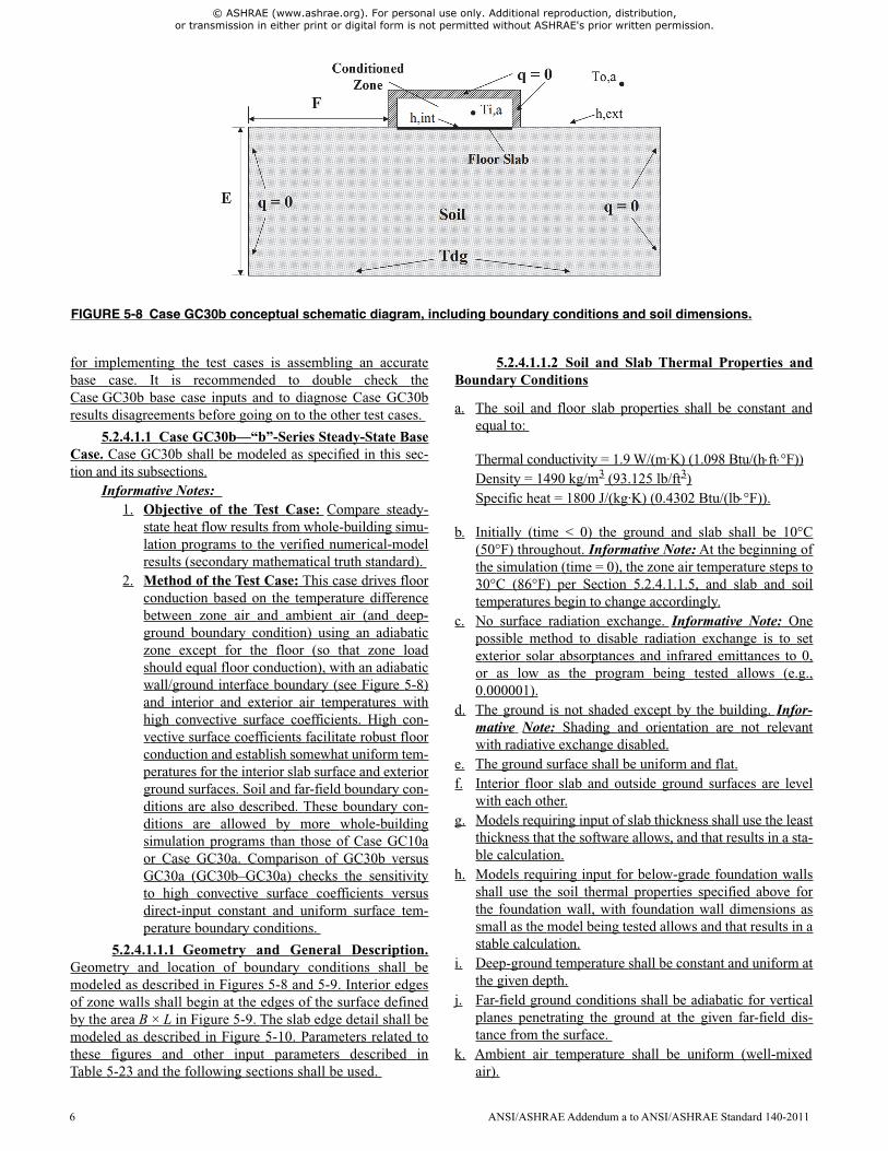
2. Method of the Test Case: This case drives floorconduction based on the temperature differencebetween zone air and ambient air (and deep-ground boundary condition) using an adiabaticzone except for the floor (so that zone loadshould equal floor conduction), with an adiabaticwall/ground interface boundary (see Figure 5-8)and interior and exterior air temperatures withhigh convective surface coefficients. High con-vective surface coefficients facilitate robust floorconduction and establish somewhat uniform tem-peratures for the interior slab surface and exteriorground surfaces. Soil and far-field boundary con-ditions are also described. These boundary con-ditions are allowed by more whole-buildingsimulation programs than those of Case GC10aor Case GC30a. Comparison of GC30b versusGC30a (GC30b–GC30a) checks the sensitivityto high convective surface coefficients versusdirect-input constant and uniform surface tem-perature boundary conditions.
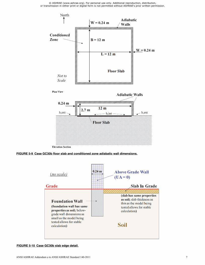
5.2.4.1.1.1 Geometry and General Description.Geometry and location of boundary conditions shall bemodeled as described in Figures 5-8 and 5-9. Interior edgesof zone walls shall begin at the edges of the surface definedby the area B × L in Figure 5-9. The slab edge detail shall bemodeled as described in Figure 5-10. Parameters related tothese figures and other input parameters described inTable 5-23 and the following sections shall be used.
5.2.4.1.1.2 Soil and Slab Thermal Properties andBoundary Conditions
a. The soil and floor slab properties shall be constant andequal to:
Thermal conductivity = 1.9 W/(m·K) (1.098 Btu/(hft°F))Density = 1490 kg/m3 (93.125 lb/ft3)Specific heat = 1800 J/(kg·K) (0.4302 Btu/(lb°F)).
b. Initially (time < 0) the ground and slab shall be 10°C(50°F) throughout. Informative Note: At the beginning ofthe simulation (time = 0), the zone air temperature steps to30°C (86°F) per Section 5.2.4.1.1.5, and slab and soiltemperatures begin to change accordingly.
c. No surface radiation exchange. Informative Note: Onepossible method to disable radiation exchange is to setexterior solar absorptances and infrared emittances to 0,or as low as the program being tested allows (e.g.,0.000001).
d. The ground is not shaded except by the building. Infor-mative Note: Shading and orientation are not relevantwith radiative exchange disabled.
e. The ground surface shall be uniform and flat.f. Interior floor slab and outside ground surfaces are level
with each other.g. Models requiring input of slab thickness shall use the least
thickness that the software allows, and that results in a sta-ble calculation.
h. Models requiring input for below-grade foundation wallsshall use the soil thermal properties specified above forthe foundation wall, with foundation wall dimensions assmall as the model being tested allows and that results in astable calculation.
i. Deep-ground temperature shall be constant and uniform atthe given depth.
j. Far-field ground conditions shall be adiabatic for verticalplanes penetrating the ground at the given far-field dis-tance from the surface.
k. Ambient air temperature shall be uniform (well-mixedair).
FIGURE 5-8 Case GC30b conceptual schematic diagram, including boundary conditions and soil dimensions.
6 ANSI/ASHRAE Addendum a to ANSI/ASHRAE Standard 140-2011
© ASHRAE (www.ashrae.org). For personal use only. Additional reproduction, distribution, or transmission in either print or digital form is not permitted without ASHRAE's prior written permission.
FIGURE 5-9 Case GC30b floor slab and conditioned zone adiabatic wall dimensions.
FIGURE 5-10 Case GC30b slab edge detail.
ANSI/ASHRAE Addendum a to ANSI/ASHRAE Standard 140-2011 7
© ASHRAE (www.ashrae.org). For personal use only. Additional reproduction, distribution, or transmission in either print or digital form is not permitted without ASHRAE's prior written permission.
l. Evapotranspiration shall not be modeled. If the programbeing tested is capable of modeling evapotranspiration, itshall be turned off or reduced to the lowest level allowedby the program.
5.2.4.1.1.3 Above-Grade Construction
a. Building height = 2.7 m (8.858 ft).b. Zone air volume = 388.8 m3 (13730 ft3).c. All surfaces of the zone except the floor are adiabatic (ther-
mal conductance = 0 W/[m2·K] [0 Btu/(h·ft2·°F)]). If theprogram being tested does not allow adiabatic surfaces, thelowest thermal conductance the program allows shall beused. Informative Note: e.g., thermal conductance =0.000001 W/(m2·K) is a sufficiently small value.
d. All surfaces except the floor are massless. If the programbeing tested does not allow massless surfaces, the lowestdensity or thermal capacitance, or both, that the programallows shall be used. Informative Note: e.g., density =0.000001 kg/m3 (0.0000001 lb/ft3) or thermal capacitance= 0.000001 J/(kg·K) (0.000001 Btu/[lb·°F]), or both, aresufficiently small values.
e. The adiabatic walls shall contact, but not penetrate, theground. Heat shall not flow between the ground and theadiabatic walls. Informative Note: Heat may flow withinthe ground just below the adiabatic walls.
f. Surface radiation exchange shall not be modeled. Infor-mative Note: One possible method to disable radiationexchange is to set interior and exterior solar absorptancesand infrared emittances to 0, or as low as the programbeing tested allows (e.g., 0.000001).
g. No windows.h. No infiltration or ventilation.i. No internal gains.
5.2.4.1.1.4 Convective Surface Coefficients
a. Interior convective surface coefficients (h,int) =100 W/(m2·K) (17.61 Btu/[h·ft2·°F]).
b. Exterior convective surface coefficients (h,ext) =100 W/(m2·K) (17.61 Btu/[h·ft2·°F]).
These values shall apply to surface coefficients for thefloor, adiabatic surfaces, and exterior ground surface. If the
program being tested cannot model these convective surfacecoefficients, the largest value the program allows shall be used.
If the program being tested allows direct user input ofconvective surface coefficients and surface infrared (IR) emit-tances, then skip the remainder of this paragraph and proceedto Section 5.2.4.1.1.5. If the program being tested allows onlydirect user input of combined surface coefficients, set thatvalue to 100 W/(m2·K) (17.61 Btu/[h·ft2·°F]). If the programbeing tested does not allow direct user input of convectivesurface coefficients or combined surface coefficients, input avalue for IR emittance such that an equivalent value for com-bined surface coefficient of 100 W/(m2·K) (17.61 Btu/[h·ft2·°F]) is obtained as closely as the program being tested iscapable of, based on the convective surface coefficient thatthe program being tested automatically calculates.
5.2.4.1.1.5 Mechanical System. The mechanicalsystem shall provide sensible heating only (no cooling). Thesystem shall be modeled as follows, as closely as the programbeing tested allows:
a. Heating setpoint = ON if temperature < 30°C (86°F); oth-erwise heat = OFF.
b. Cooling setpoint = always OFF.c. The heating system capacity shall be large enough to
maintain the zone air temperature setpoint. InformativeNote: For example, 1000 kW (3412 kBtu/h). InformativeNote: This specification for the heating capacity isrepeated for steady-state cases where floor conduction ofthe verified numerical models is greater for the given casethan for its designated base case.
d. Uniform zone air temperature (well-mixed air).e. 100% efficiency.f. 100% convective air system.g. Ideal controls with the zone air temperature always at the
thermostat setpoint. Informative Note: For example,assume the heat addition rate equals the equipment capac-ity (nonproportional control) and there is continuous ON/OFF cycling within the hour as needed.
h. The thermostat shall sense the zone air temperature only.
Informative Note: The purpose of this idealized heatingsystem is to give results for energy consumption that areequal to the sensible heating load.
5.2.4.1.1.6 Weather Data. The constant temperatureTMY2 format weather data provided with the following file,included on the accompanying electronic media, shall beused: GC30b.TM2.
If the program does not utilize site data from the weatherdata file, the site parameters provided in normativeAnnex A1, Section A1.1.2 shall be used.
Informative Note: Supporting details for this weatherdata are provided in Annex A1, Section A1.1.2. Other casescall for different weather files as needed.
5.2.4.1.1.7 Modeling Precision
5.2.4.1.1.7.1 Simulation Duration. The simula-tion shall be run until there is 0.1% variation between thefloor slab conduction for the last hour of the last year of thesimulation and the last hour of the preceding year of the simu-lation. If the software being tested is not capable of this, the
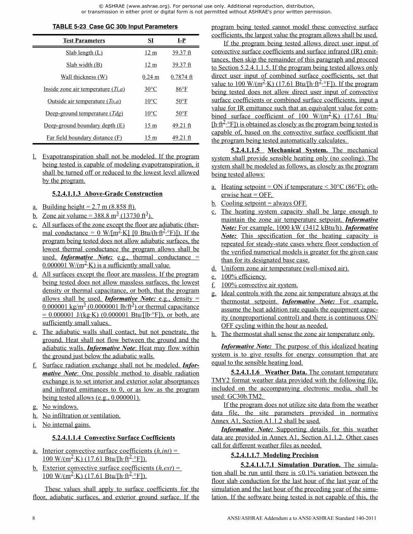
TABLE 5-23 Case GC 30b Input Parameters
Test Parameters SI I-P
Slab length (L) 12 m 39.37 ft
Slab width (B) 12 m 39.37 ft
Wall thickness (W) 0.24 m 0.7874 ft
Inside zone air temperature (Ti,a) 30°C 86°F
Outside air temperature (To,a) 10°C 50°F
Deep-ground temperature (Tdg) 10°C 50°F
Deep-ground boundary depth (E) 15 m 49.21 ft
Far field boundary distance (F) 15 m 49.21 ft
8 ANSI/ASHRAE Addendum a to ANSI/ASHRAE Standard 140-2011
© ASHRAE (www.ashrae.org). For personal use only. Additional reproduction, distribution, or transmission in either print or digital form is not permitted without ASHRAE's prior written permission.
simulation duration shall be for as long as the software beingtested is capable of running.
Informative Notes:1. Thermal Node Mesh: If the numerical
model being tested allows variation of ther-mal node meshing, it is recommended todemonstrate for a subset of the steady-stateand steady-periodic cases (e.g., GC30b,GC40b, and others if desired) that thetested mesh detail yields negligible (0.1%)change in results versus a less detailedmesh, or that the mesh is as detailed as pos-sible for the available computing hardware.
2. Convergence Tolerance: If the softwarebeing tested allows user specification ofconvergence tolerance, it is recommendedto demonstrate for a subset of the steady-state and steady-periodic cases (e.g.,GC30b and GC40b) that the current level ofheat-flow or temperature convergence toler-ance yields negligible (0.1%) change inresults versus the next finer convergencetolerance.
5.2.4.1.1.8 Output Requirements. Output shall beprovided in accordance with Section 6.2.2.1.
5.2.4.1.2 Case GC40b—Harmonic Variation ofAmbient Temperature. Case GC40b shall be modeled asspecified in this section.
Informative Notes:1. Objective of the Test Case: Compare heat flow
results for approximate steady-periodic (har-monic) variation of ambient temperature (To,a)from whole-building simulation programs versusverified numerical-model results. Analyze thephase shift between variations of heat flow andambient air temperature.
2. Method of the Test Case: This case is similar toCase GC30b but uses harmonically varying To,a.Hourly TMY2 format weather data are providedfor approximating a sinusoidal annual cycle ofvarying daily average temperatures with a sinu-soidal diurnal temperature cycle overlaid (a highfrequency cycle overlaid on a low frequencycycle). Comparing GC40b with GC30b (GC40b–GC30b) annual hourly average floor conductionchecks the sensitivity of average floor heat lossof the harmonic condition versus the steady-statecondition.
5.2.4.1.2.1 Input Specification. This case shall bemodeled exactly as Case GC30b except for the followingchanges:
a. Weather Data. The weather data provided with the fol-lowing file, included on the accompanying electronicmedia, shall be used: GC40b.TM2.
If the program does not utilize site data from theweather data file, the site parameters provided in norma-tive Annex A1, Section A1.1.2 shall be used.
Informative Note: These data are described inAnnex A1, Section A1.1.2; see Section A1.1.2.1 regard-ing harmonically varying inputs.
b. Heating System Capacity. The heating system capacityshall be set so there is at least enough capacity to maintainthe zone air temperature setpoint during the peak heating-load hour. Informative Note: The heating capacity mayvary among the test cases. This specification for the heat-ing capacity is repeated for harmonically varying caseswhere floor conduction of the verified numerical modelsis greater for the given case than for its designated basecase.
c. Simulation Duration. The simulation shall be run untilthere is 0.1% variation between the annual floor slabconduction for the last year of the simulation and the pre-ceding year of the simulation. If the software being testedis not capable of this, the simulation duration shall be foras long as the software being tested is capable of running.
5.2.4.1.2.2 Output Requirements. Output shall beprovided in accordance with Section 6.2.2.2.
5.2.4.1.3 Case GC45b—Aspect Ratio. Case GC45bshall be modeled as specified in this section.
Informative Notes:1. Objective of the Test Case: Test the sensitivity
to variation of aspect ratio (AR) in the context ofsteady-periodic (harmonic) variation of To,a. TheAR for a given slab area directly affects the ratioof perimeter heat transfer to core heat transfer. Inthis context the use of the term perimeter is dif-ferent from the perimeter boundary described inCase GC10a. Here, perimeter heat transfer is theheat transfer driven by the zone-to-ambient airtemperature difference through a relatively thinlayer of soil; core heat transfer is driven by thezone-to-deep-ground temperature difference,through a relatively thick layer of soil.
2. Method of the Test Case: This case is similar toCase GC40b. It uses a slab with same surfacearea but different AR. Comparison of results forGC45b versus GC40b (GC45b-GC40b) checksthe sensitivity of AR. Compare heat-flow resultsfrom whole-building simulation programs to ver-ified numerical-model results. Analyze phaseshift between variations of heat flow and To,a.
5.2.4.1.3.1 Input Specification. This case shall bemodeled exactly as Case GC40b except for the followingchanges:
a. Slab Dimensions. The slab dimensions shall be modeledas specified in Table 5-24.
b. Heating System Capacity. The heating system capacityshall be modeled as needed so there is at least enoughcapacity to maintain the zone air temperature setpoint dur-ing the peak heating-load hour.
5.2.4.1.3.2 Output Requirements. Output shall beprovided in accordance with Section 6.2.2.2 except slabdimensions L and B from Table 5-24 shall be used.
ANSI/ASHRAE Addendum a to ANSI/ASHRAE Standard 140-2011 9
© ASHRAE (www.ashrae.org). For personal use only. Additional reproduction, distribution, or transmission in either print or digital form is not permitted without ASHRAE's prior written permission.
5.2.4.1.4 Case GC50b—Large Slab. Case GC50bshall be modeled as specified in this section.
Informative Notes:
1. Objective of the Test Case: Test the sensitivityto variation of slab size in the context of steady-periodic (harmonic) variation of To,a. Increasingthe slab size yields a larger fraction of core-driven ground heat transfer that is driven by thedifference between the zone air temperature andthe deep-ground temperature.
2. Method of the Test Case: This case is similar toCase GC40b but uses a large slab. Comparingresults for heat flow per unit floor area (flux) forGC50b versus GC40b (GC50b–GC40b) checksthe sensitivity to heat transfer caused by increas-ing the slab size. Compare heat-flow results fromwhole-building simulation programs to verifiednumerical-model results. Analyze phase shiftbetween variations of heat flow and To,a.
5.2.4.1.4.1 Input Specification. This case shall be mod-eled exactly as Case GC40b except for the following changes:
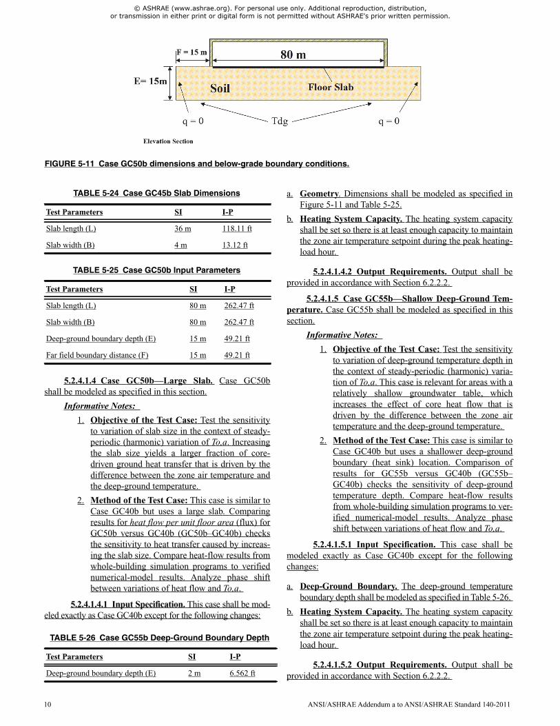
a. Geometry. Dimensions shall be modeled as specified inFigure 5-11 and Table 5-25.
b. Heating System Capacity. The heating system capacityshall be set so there is at least enough capacity to maintainthe zone air temperature setpoint during the peak heating-load hour.
5.2.4.1.4.2 Output Requirements. Output shall beprovided in accordance with Section 6.2.2.2.
5.2.4.1.5 Case GC55b—Shallow Deep-Ground Tem-perature. Case GC55b shall be modeled as specified in thissection.
Informative Notes:
1. Objective of the Test Case: Test the sensitivityto variation of deep-ground temperature depth inthe context of steady-periodic (harmonic) varia-tion of To,a. This case is relevant for areas with arelatively shallow groundwater table, whichincreases the effect of core heat flow that isdriven by the difference between the zone airtemperature and the deep-ground temperature.
2. Method of the Test Case: This case is similar toCase GC40b but uses a shallower deep-groundboundary (heat sink) location. Comparison ofresults for GC55b versus GC40b (GC55b–GC40b) checks the sensitivity of deep-groundtemperature depth. Compare heat-flow resultsfrom whole-building simulation programs to ver-ified numerical-model results. Analyze phaseshift between variations of heat flow and To,a.
5.2.4.1.5.1 Input Specification. This case shall bemodeled exactly as Case GC40b except for the followingchanges:
a. Deep-Ground Boundary. The deep-ground temperatureboundary depth shall be modeled as specified in Table 5-26.
b. Heating System Capacity. The heating system capacityshall be set so there is at least enough capacity to maintainthe zone air temperature setpoint during the peak heating-load hour.
5.2.4.1.5.2 Output Requirements. Output shall beprovided in accordance with Section 6.2.2.2.
TABLE 5-24 Case GC45b Slab Dimensions
Test Parameters SI I-P
Slab length (L) 36 m 118.11 ft
Slab width (B) 4 m 13.12 ft
TABLE 5-25 Case GC50b Input Parameters
Test Parameters SI I-P
Slab length (L) 80 m 262.47 ft
Slab width (B) 80 m 262.47 ft
Deep-ground boundary depth (E) 15 m 49.21 ft
Far field boundary distance (F) 15 m 49.21 ft
TABLE 5-26 Case GC55b Deep-Ground Boundary Depth
Test Parameters SI I-P
Deep-ground boundary depth (E) 2 m 6.562 ft
FIGURE 5-11 Case GC50b dimensions and below-grade boundary conditions.
10 ANSI/ASHRAE Addendum a to ANSI/ASHRAE Standard 140-2011
© ASHRAE (www.ashrae.org). For personal use only. Additional reproduction, distribution, or transmission in either print or digital form is not permitted without ASHRAE's prior written permission.
5.2.4.1.6 Case GC60b—Steady State with TypicalInterior Convective Surface Coefficient. Case GC60b shallbe modeled as specified in this section.
Informative Notes:1. Objective of the Test Case: Test sensitivity to
the use of a more realistic interior convective sur-face heat transfer coefficient (h,int) in the steady-state context. With a more realistic coefficient,the zone floor surface temperature will be lessuniform and will exhibit greater decrease out-ward from the center toward the zone perimeterboundary.
2. Method of the Test Case: This case is similar toCase GC30b but uses decreased h,int. Compari-son of results for GC60b versus GC30b (GC60b–GC30b) checks the sensitivity of h,int. Compareheat-flow results from whole-building simulationprograms to verified numerical-model results.
5.2.4.1.6.1 Input Specification. This case shall bemodeled exactly as Case GC30b except for the followingchanges:
a. Interior Convective Surface Coefficient. The value forh,int shall be modeled as specified in Table 5-27. Thisvalue of h,int shall be applied to the interior side of thefloor and other zone surfaces (i.e., walls and ceiling).
Surface IR emittances shall be modeled as 0 (or as lowas the program being tested allows). If the program beingtested allows direct user input of interior convective sur-face coefficients and interior surface IR emittances, thenskip the remainder of this paragraph and proceed to Sec-tion 5.2.4.1.6.2. If the program being tested allows directuser input of combined interior surface coefficients only,set that value to 7.95 W/(m2·K) (1.3999 Btu/[h·ft2·°F]). Ifthe program being tested does not allow direct user inputof convective surface coefficients or combined surfacecoefficients, input a value for IR emittance such that anequivalent value for a combined surface coefficient of7.95 W/(m2·K) (1.3999 Btu/[h·ft2·°F]) is obtained asclosely as the program being tested is capable of, based onthe convective surface coefficient that the program beingtested automatically calculates.
5.2.4.1.6.2 Output Requirements. Output shall beprovided in accordance with Section 6.2.2.1.
5.2.4.1.7 Case GC65b—Steady State with TypicalInterior and Exterior Convective Surface Coefficients.Case GC65b shall be modeled as specified in this section.
Informative Notes:1. Objective of the Test Case: Test sensitivity to
the use of a more realistic exterior convectivesurface coefficient (h,ext) in the steady-state con-text. With a more realistic coefficient, the exte-rior ground surface temperature will be lessuniform and will exhibit greater increase near theexterior side of the adiabatic wall.
2. Method of the Test Case: This case is similar toCase GC60b but uses decreased h,ext. Compari-son of results for GC65b versus GC60b (GC65b–
GC60b) checks the sensitivity of h,ext. Compari-son of results for GC65b versus GC30b (GC65b–GC30b) checks the combined effect of sensitivityto h,int and h,ext. Compare heat-flow resultsfrom whole-building simulation programs to ver-ified numerical-model results.
5.2.4.1.7.1 Input Specification. This case shall bemodeled exactly as Case GC60b except for the followingchanges:
a. Exterior Convective Surface Coefficient. The value forh,ext shall be modeled as specified in Table 5-28. Thisvalue of h,ext shall be applied to the exterior ground sur-face and to other zone exterior surfaces (i.e., walls andceiling). Informative Note: The value for h,int is repeatedin Table 5-28 for convenience.
Surface IR emittances shall be modeled as 0 (or as lowas the program being tested allows). If the program beingtested allows direct user input of h,ext and exterior surfaceIR emittances, then skip the remainder of this paragraphand proceed to Section 5.2.4.1.7.1, item b (just below). Ifthe program being tested allows direct user input of com-bined exterior surface coefficients only, set that value to11.95 W/(m2·K) (2.1043 Btu/[h·ft2·°F]). If the programbeing tested does not allow direct user input of convectivesurface coefficients or combined surface coefficients, inputa value for IR emittance such that an equivalent value forcombined surface coefficient of 11.95 W/(m2·K) (2.1043Btu/[h·ft2·°F]) is obtained as closely as the program beingtested is capable of, based on the convective surface coef-ficient that the program being tested automatically calcu-lates.
b. Weather Data. The weather data provided with the fol-lowing file, included on the accompanying electronicmedia, shall be used: GC65b.TM2.
If the program does not utilize site data from theweather data file, the site parameters provided in norma-tive Annex A1, Section A1.1.2 shall be used.
5.2.4.1.7.2 Output Requirements. Output shall beprovided in accordance with Section 6.2.2.1.
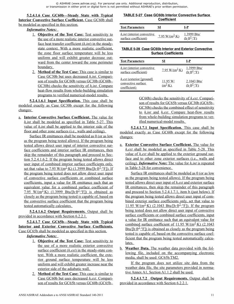
TABLE 5-27 Case GC60b Interior Convective SurfaceCoefficient
Test Parameters SI I-P
h,int (interior convectivesurface coefficient)
7.95 W/(m2·K)1.3999 Btu/(h·ft2·°F)
TABLE 5-28 Case GC65b Interior and Exterior ConvectiveSurface Coefficients
Test Parameters SI I-P
h,int (interior convectivesurface coefficient)
7.95 W/(m2·K)1.3999 Btu/(h·ft2·°F)
h,ext (exterior [ground]convective surfacecoefficient)
11.95 W/(m2·K)
2.1043 Btu/(h·ft2·°F)
ANSI/ASHRAE Addendum a to ANSI/ASHRAE Standard 140-2011 11
© ASHRAE (www.ashrae.org). For personal use only. Additional reproduction, distribution, or transmission in either print or digital form is not permitted without ASHRAE's prior written permission.
5.2.4.1.8 Case GC70b—Harmonic Variation ofAmbient Temperature with Typical Interior and ExteriorConvective Surface Coefficients. Case GC70b shall be mod-eled as specified in this section.
Informative Notes:1. Objective of the Test Case: Test sensitivity to
the use of more realistic h,int and h,ext in thecontext of steady-periodic (harmonic) variationof To,a.
2. Method of the Test Case: This case is similar toCase GC40b but uses decreased h,int and h,ext.Comparison of results for GC70b versus GC40b(GC70b–GC40b) checks the combined sensitivi-ties of h,int and h,ext. Compare heat-flow resultsfrom whole-building simulation programs to ver-ified numerical-model results. Analyze phaseshift between variations of heat flow and To,a.Comparison of GC70b versus GC65b (GC70b–GC65b) annual hourly average floor conductionchecks the sensitivity of average floor heat lossof the harmonic versus the steady-state conditionin the context of using realistic convective sur-face coefficients.
5.2.4.1.8.1 Input Specification. This case shall bemodeled exactly as Case GC40b except for the followingchanges:
a. Convective Surface Coefficients. h,int and h,ext shall bemodeled as specified in Table 5-28 (seeSection 5.2.4.1.7.1).
b. Weather Data. The weather provided with the followingfile, included on the accompanying electronic media, shallbe used: GC70b.TM2.
If the program does not utilize site data from theweather data file, the site parameters provided in norma-tive Annex A1, Section A1.1.2 shall be used.
Informative Note: See Annex A1, Section A1.1.2.1regarding harmonically varying inputs.
5.2.4.1.8.2 Output Requirements. Output shall beprovided in accordance with Section 6.2.2.2.
5.2.4.1.9 Case GC80b—Reduced Slab and GroundConductivity. Case GC80b shall be modeled as specified inthis section.
Informative Notes:1. Objective of the Test Case: Test sensitivity to
reduced slab and ground conductivity in the con-text of steady-periodic (harmonic) variation ofTo,a.
2. Method of the Test Case: This case is similar toCase GC40b but uses decreased slab and groundconductivity. Comparison of results for GC80bversus GC40b (GC80b–GC40b) checks the sen-sitivity of slab and ground conductivity. Com-pare heat-flow results from whole-buildingsimulation programs to verified numerical-modelresults. Analyze phase shift between variationsof heat flow and To,a.
5.2.4.1.9.1 Input Specification. This case shall bemodeled exactly as Case GC40b except for the followingchange:
Soil and slab thermal conductivity = 0.5 W/(m·K) (0.289 Btu/[h·ft·°F])
5.2.4.1.9.2 Output Requirements. Output shall beprovided in accordance with Section 6.2.2.2.
5.2.4.2 “a”-Series Cases. The “a”-series cases shall bemodeled as specified in this section. Case GC10a shall be thefirst case modeled and all other tests in this series shall besequential revisions to a previously completed model. Thebase case models for each case shall be:
Informative Note: The “a”-series cases are for detailednumerical-methods programs (e.g., three-dimensional [3D]numerical models) that are either integrated within or runindependently from whole-building energy simulation pro-grams. Within the “a”-series cases, Case GC10a provides a3D steady-state analytical solution for rectangular surfacegeometry (Delsante, Stokes, and Walsh 1983).A-4
5.2.4.2.1 Case GC10a Analytical Solution Case. CaseGC10a shall be modeled as specified in this section.
Informative Notes:1. Objective of the Test Case: Compare steady-
state heat flow results for detailed 3D numericalmodels used independently from whole-buildingenergy simulation programs versus an analyticalsolution (described in Annex B11, SectionB11.2.1). Users of such detailed models are todetermine appropriate inputs to match the bound-ary conditions and assumptions of the analyticalsolution, including appropriate meshing, theamount of ground that needs to be modeled, andlength of simulation, etc. Attention to such mod-eling details is needed to obtain consistent high-quality results throughout these test cases. Inother test cases where exact analytical solutionsare not known—and if there is good agreementamong detailed numerical models and appropri-ate application of the models is well docu-mented—the detailed numerical-model resultscan be used as verified numerical model results.Such results provide a secondary mathematicaltruth standard, founded on the range of disagree-ment of the verified numerical-model results, forcomparing results of other models typically usedwith whole-building energy simulation pro-grams.
2. Method of the Test Case: This case calculatessteady-state heat flow using fundamental 3D heat
Case Basis for Case
GC10a Not Applicable
GC30a GC30b
GC40a GC30a
12 ANSI/ASHRAE Addendum a to ANSI/ASHRAE Standard 140-2011
© ASHRAE (www.ashrae.org). For personal use only. Additional reproduction, distribution, or transmission in either print or digital form is not permitted without ASHRAE's prior written permission.
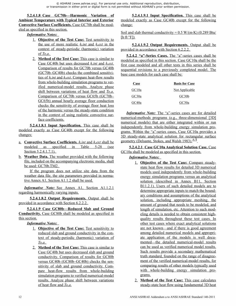
transfer analysis of a semi-infinite solid.A-4, A-8
Figure 5-12 shows the boundary conditions at theupper surface of the semi-infinite solid anddescribes a rectangular floor surface bounded bya concentrically rectangular perimeter surface offinite width that separates the rectangular floorsurface from the exterior ground surface. Theconcentrically rectangular surface may also bethought of as the base of a wall that separates theinterior floor surface from the exterior groundsurface. Required boundary conditions may limitthe number of models that can run this test case.It is recommended to check sensitivity to meshdetail, length of simulation, amount of groundmodeled, convergence tolerance, etc., and dem-onstrate that the model is at a level of detailwhere including further detail yields negligiblesensitivity to results.
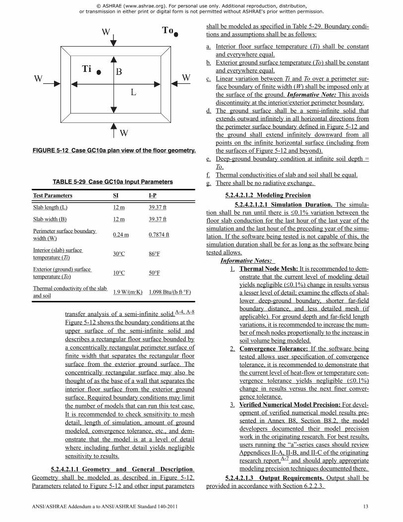
5.2.4.2.1.1 Geometry and General Description.Geometry shall be modeled as described in Figure 5-12.Parameters related to Figure 5-12 and other input parameters
shall be modeled as specified in Table 5-29. Boundary condi-tions and assumptions shall be as follows:
a. Interior floor surface temperature (Ti) shall be constantand everywhere equal.
b. Exterior ground surface temperature (To) shall be constantand everywhere equal.
c. Linear variation between Ti and To over a perimeter sur-face boundary of finite width (W) shall be imposed only atthe surface of the ground. Informative Note: This avoidsdiscontinuity at the interior/exterior perimeter boundary.
d. The ground surface shall be a semi-infinite solid thatextends outward infinitely in all horizontal directions fromthe perimeter surface boundary defined in Figure 5-12 andthe ground shall extend infinitely downward from allpoints on the infinite horizontal surface (including fromthe surfaces of Figure 5-12 and beyond).
e. Deep-ground boundary condition at infinite soil depth =To.
f. Thermal conductivities of slab and soil shall be equal.g. There shall be no radiative exchange.
5.2.4.2.1.2 Modeling Precision
5.2.4.2.1.2.1 Simulation Duration. The simula-tion shall be run until there is 0.1% variation between thefloor slab conduction for the last hour of the last year of thesimulation and the last hour of the preceding year of the simu-lation. If the software being tested is not capable of this, thesimulation duration shall be for as long as the software beingtested allows.
Informative Notes:1. Thermal Node Mesh: It is recommended to dem-
onstrate that the current level of modeling detailyields negligible (0.1%) change in results versusa lesser level of detail; examine the effects of shal-lower deep-ground boundary, shorter far-fieldboundary distance, and less detailed mesh (ifapplicable). For ground depth and far-field lengthvariations, it is recommended to increase the num-ber of mesh nodes proportionally to the increase insoil volume being modeled.
2. Convergence Tolerance: If the software beingtested allows user specification of convergencetolerance, it is recommended to demonstrate thatthe current level of heat-flow or temperature con-vergence tolerance yields negligible (0.1%)change in results versus the next finer conver-gence tolerance.
3. Verified Numerical Model Precision: For devel-opment of verified numerical model results pre-sented in Annex B8, Section B8.2, the modeldevelopers documented their model precisionwork in the originating research. For best results,users running the “a”-series cases should reviewAppendices II-A, II-B, and II-C of the originatingresearch report,A-7 and should apply appropriatemodeling precision techniques documented there.
5.2.4.2.1.3 Output Requirements. Output shall beprovided in accordance with Section 6.2.2.3.
TABLE 5-29 Case GC10a Input Parameters
Test Parameters SI I-P
Slab length (L) 12 m 39.37 ft
Slab width (B) 12 m 39.37 ft
Perimeter surface boundarywidth (W)
0.24 m 0.7874 ft
Interior (slab) surfacetemperature (Ti)
30°C 86°F
Exterior (ground) surfacetemperature (To)
10°C 50°F
Thermal conductivity of the slaband soil
1.9 W/(m·K) 1.098 Btu/(hft°F)
FIGURE 5-12 Case GC10a plan view of the floor geometry.
ANSI/ASHRAE Addendum a to ANSI/ASHRAE Standard 140-2011 13
© ASHRAE (www.ashrae.org). For personal use only. Additional reproduction, distribution, or transmission in either print or digital form is not permitted without ASHRAE's prior written permission.
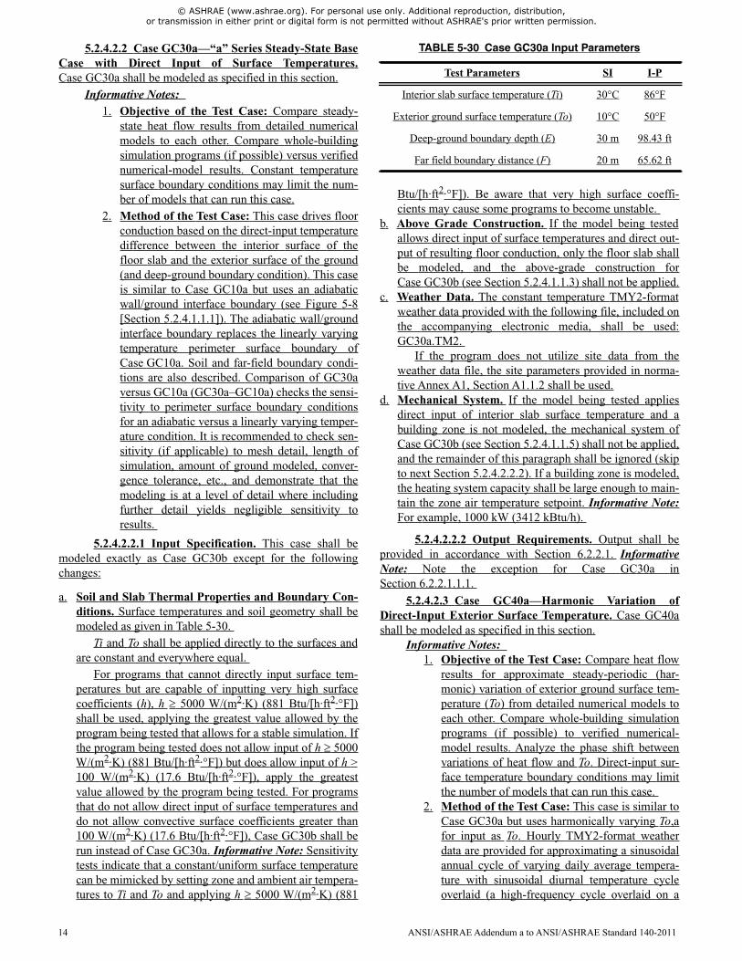
5.2.4.2.2 Case GC30a—“a” Series Steady-State BaseCase with Direct Input of Surface Temperatures.Case GC30a shall be modeled as specified in this section.
Informative Notes:1. Objective of the Test Case: Compare steady-
state heat flow results from detailed numericalmodels to each other. Compare whole-buildingsimulation programs (if possible) versus verifiednumerical-model results. Constant temperaturesurface boundary conditions may limit the num-ber of models that can run this case.
2. Method of the Test Case: This case drives floorconduction based on the direct-input temperaturedifference between the interior surface of thefloor slab and the exterior surface of the ground(and deep-ground boundary condition). This caseis similar to Case GC10a but uses an adiabaticwall/ground interface boundary (see Figure 5-8[Section 5.2.4.1.1.1]). The adiabatic wall/groundinterface boundary replaces the linearly varyingtemperature perimeter surface boundary ofCase GC10a. Soil and far-field boundary condi-tions are also described. Comparison of GC30aversus GC10a (GC30a–GC10a) checks the sensi-tivity to perimeter surface boundary conditionsfor an adiabatic versus a linearly varying temper-ature condition. It is recommended to check sen-sitivity (if applicable) to mesh detail, length ofsimulation, amount of ground modeled, conver-gence tolerance, etc., and demonstrate that themodeling is at a level of detail where includingfurther detail yields negligible sensitivity toresults.
5.2.4.2.2.1 Input Specification. This case shall bemodeled exactly as Case GC30b except for the followingchanges:
a. Soil and Slab Thermal Properties and Boundary Con-ditions. Surface temperatures and soil geometry shall bemodeled as given in Table 5-30.
Ti and To shall be applied directly to the surfaces andare constant and everywhere equal.
For programs that cannot directly input surface tem-peratures but are capable of inputting very high surfacecoefficients (h), h 5000 W/(m2·K) (881 Btu/[h·ft2·°F])shall be used, applying the greatest value allowed by theprogram being tested that allows for a stable simulation. Ifthe program being tested does not allow input of h 5000W/(m2·K) (881 Btu/[h·ft2·°F]) but does allow input of h >100 W/(m2·K) (17.6 Btu/[h·ft2·°F]), apply the greatestvalue allowed by the program being tested. For programsthat do not allow direct input of surface temperatures anddo not allow convective surface coefficients greater than100 W/(m2·K) (17.6 Btu/[h·ft2·°F]), Case GC30b shall berun instead of Case GC30a. Informative Note: Sensitivitytests indicate that a constant/uniform surface temperaturecan be mimicked by setting zone and ambient air tempera-tures to Ti and To and applying h 5000 W/(m2·K) (881
Btu/[h·ft2·°F]). Be aware that very high surface coeffi-cients may cause some programs to become unstable.
b. Above Grade Construction. If the model being testedallows direct input of surface temperatures and direct out-put of resulting floor conduction, only the floor slab shallbe modeled, and the above-grade construction forCase GC30b (see Section 5.2.4.1.1.3) shall not be applied.
c. Weather Data. The constant temperature TMY2-formatweather data provided with the following file, included onthe accompanying electronic media, shall be used:GC30a.TM2.
If the program does not utilize site data from theweather data file, the site parameters provided in norma-tive Annex A1, Section A1.1.2 shall be used.
d. Mechanical System. If the model being tested appliesdirect input of interior slab surface temperature and abuilding zone is not modeled, the mechanical system ofCase GC30b (see Section 5.2.4.1.1.5) shall not be applied,and the remainder of this paragraph shall be ignored (skipto next Section 5.2.4.2.2.2). If a building zone is modeled,the heating system capacity shall be large enough to main-tain the zone air temperature setpoint. Informative Note:For example, 1000 kW (3412 kBtu/h).
5.2.4.2.2.2 Output Requirements. Output shall beprovided in accordance with Section 6.2.2.1. InformativeNote: Note the exception for Case GC30a inSection 6.2.2.1.1.1.
5.2.4.2.3 Case GC40a—Harmonic Variation ofDirect-Input Exterior Surface Temperature. Case GC40ashall be modeled as specified in this section.
Informative Notes:1. Objective of the Test Case: Compare heat flow
results for approximate steady-periodic (har-monic) variation of exterior ground surface tem-perature (To) from detailed numerical models toeach other. Compare whole-building simulationprograms (if possible) to verified numerical-model results. Analyze the phase shift betweenvariations of heat flow and To. Direct-input sur-face temperature boundary conditions may limitthe number of models that can run this case.
2. Method of the Test Case: This case is similar toCase GC30a but uses harmonically varying To,afor input as To. Hourly TMY2-format weatherdata are provided for approximating a sinusoidalannual cycle of varying daily average tempera-ture with sinusoidal diurnal temperature cycleoverlaid (a high-frequency cycle overlaid on a
TABLE 5-30 Case GC30a Input Parameters
Test Parameters SI I-P
Interior slab surface temperature (Ti) 30°C 86°F
Exterior ground surface temperature (To) 10°C 50°F
Deep-ground boundary depth (E) 30 m 98.43 ft
Far field boundary distance (F) 20 m 65.62 ft
14 ANSI/ASHRAE Addendum a to ANSI/ASHRAE Standard 140-2011
© ASHRAE (www.ashrae.org). For personal use only. Additional reproduction, distribution, or transmission in either print or digital form is not permitted without ASHRAE's prior written permission.
low-frequency cycle). Comparison of GC40aversus GC30a (GC40a–GC30a) annual hourlyaverage floor conduction checks the sensitivityof average floor heat loss of the harmonic condi-tion versus the steady-state condition. It is rec-ommended to check sensitivity (if applicable) tomesh detail, length of simulation, amount ofground modeled, convergence tolerance, etc.,and demonstrate that the modeling is at a level ofdetail where including further detail yields negli-gible sensitivity to results.
5.2.4.2.3.1 Input Specification. This case is exactlyas Case GC30a except for the following changes:
a. Weather Data. The weather data provided with the fol-lowing file, included on the accompanying electronicmedia, shall be used: GC40a.TM2.
If the program does not utilize site data from theweather data file, the site parameters provided in norma-tive Annex A1, Section A1.1.2 shall be used.
Informative Note: These data are described in Annex A1,Section A1.1.2; see Section A1.1.2.1 regarding harmonicallyvarying inputs.
b. Heating System Capacity. If the model being testedapplies direct input of interior slab surface temperatureand a building zone is not modeled, the mechanical sys-tem of Case GC30b (see Section 5.2.4.1.1.5) shall not beapplied, and the remainder of this paragraph shall beignored (skip to next bullet item, Section 5.2.4.2.3.1[c]).If a building zone is modeled, the heating system capacityshall be set so there is at least enough capacity to maintainthe zone air temperature setpoint during the peak heating-load hour.
c. Simulation Duration. The simulation shall be run untilthere is 0.1% variation between the annual floor slabconduction for the last year of the simulation and the pre-ceding year of the simulation. If the software being testedis not capable of this, the simulation duration shall be foras long as the software being tested is capable of running.
5.2.4.2.3.2 Output Requirements. Output shall beprovided in accordance with Section 6.2.2.2. InformativeNote: Note the Case GC40a exception in Section 6.2.2.2.2.1.
5.2.4.3 “c”-Series Cases. The “c”-series cases shall bemodeled as specified in this section. Case GC30c shall be thefirst modeled, and all other tests in this series shall be sequen-tial revisions to a previously completed model. The base casemodels for each case shall be:
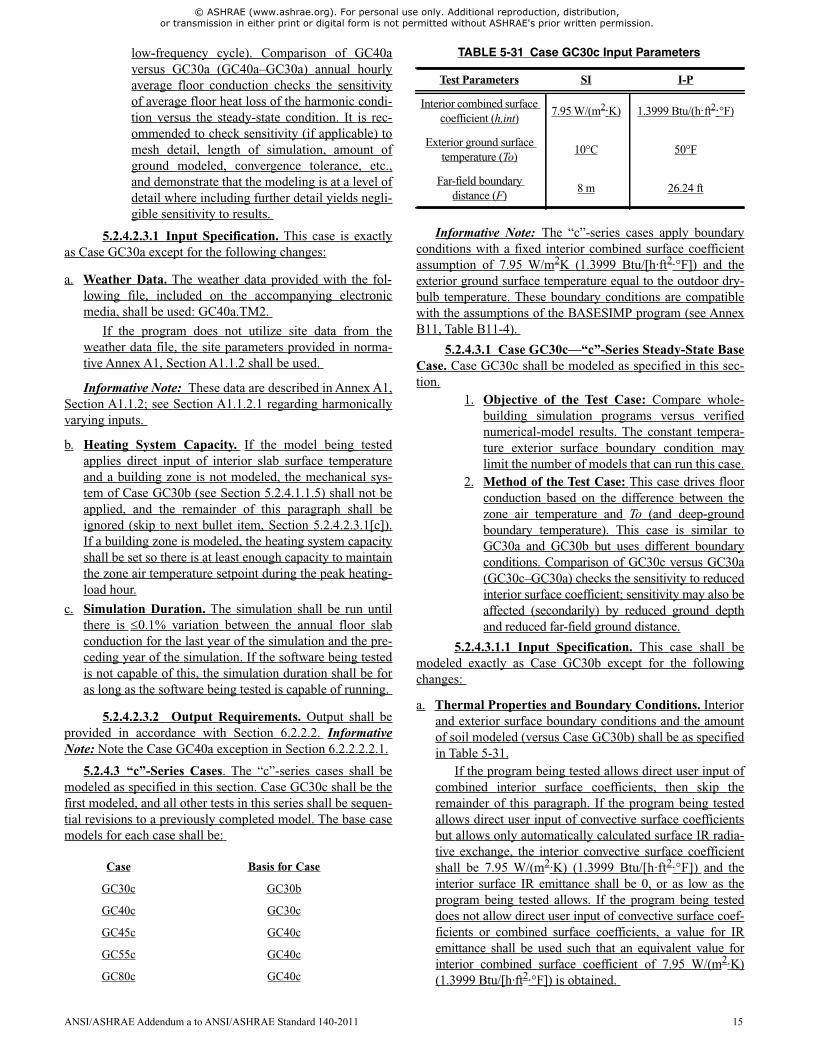
Informative Note: The “c”-series cases apply boundaryconditions with a fixed interior combined surface coefficientassumption of 7.95 W/m2K (1.3999 Btu/[h·ft2·°F]) and theexterior ground surface temperature equal to the outdoor dry-bulb temperature. These boundary conditions are compatiblewith the assumptions of the BASESIMP program (see AnnexB11, Table B11-4).
5.2.4.3.1 Case GC30c—“c”-Series Steady-State BaseCase. Case GC30c shall be modeled as specified in this sec-tion.
1. Objective of the Test Case: Compare whole-building simulation programs versus verifiednumerical-model results. The constant tempera-ture exterior surface boundary condition maylimit the number of models that can run this case.
2. Method of the Test Case: This case drives floorconduction based on the difference between thezone air temperature and To (and deep-groundboundary temperature). This case is similar toGC30a and GC30b but uses different boundaryconditions. Comparison of GC30c versus GC30a(GC30c–GC30a) checks the sensitivity to reducedinterior surface coefficient; sensitivity may also beaffected (secondarily) by reduced ground depthand reduced far-field ground distance.
5.2.4.3.1.1 Input Specification. This case shall bemodeled exactly as Case GC30b except for the followingchanges:
a. Thermal Properties and Boundary Conditions. Interiorand exterior surface boundary conditions and the amountof soil modeled (versus Case GC30b) shall be as specifiedin Table 5-31.
If the program being tested allows direct user input ofcombined interior surface coefficients, then skip theremainder of this paragraph. If the program being testedallows direct user input of convective surface coefficientsbut allows only automatically calculated surface IR radia-tive exchange, the interior convective surface coefficientshall be 7.95 W/(m2·K) (1.3999 Btu/[h·ft2·°F]) and theinterior surface IR emittance shall be 0, or as low as theprogram being tested allows. If the program being testeddoes not allow direct user input of convective surface coef-ficients or combined surface coefficients, a value for IRemittance shall be used such that an equivalent value forinterior combined surface coefficient of 7.95 W/(m2·K)(1.3999 Btu/[h·ft2·°F]) is obtained.
Case Basis for Case
GC30c GC30b
GC40c GC30c
GC45c GC40c
GC55c GC40c
GC80c GC40c
TABLE 5-31 Case GC30c Input Parameters
Test Parameters SI I-P
Interior combined surfacecoefficient (h,int)
7.95 W/(m2·K) 1.3999 Btu/(h·ft2·°F)
Exterior ground surfacetemperature (To)
10°C 50°F
Far-field boundarydistance (F)
8 m 26.24 ft
ANSI/ASHRAE Addendum a to ANSI/ASHRAE Standard 140-2011 15
© ASHRAE (www.ashrae.org). For personal use only. Additional reproduction, distribution, or transmission in either print or digital form is not permitted without ASHRAE's prior written permission.
Exterior ground surface temperature (To) shall beapplied directly to the surface and shall be constant andeverywhere equal.
For programs that cannot directly input To but are capa-ble of inputting very high h,ext, h,ext 5000 W/(m2·K)(881 Btu/[h·ft2·°F]) shall be used, applying the greatestvalue that the program being tested allows for a stable simu-lation. If the program being tested does not allow input ofh,ext 5000 W/(m2·K) (881 Btu/[h·ft2·°F]), the greatestvalue allowed by the program being tested shall be used.Informative Note: Sensitivity tests indicate that a constant/uniform surface temperature can be mimicked by settingTo,a to To and applying h,ext 5000 W/(m2·K) (881 Btu/[h·ft2·°F]). Be aware that very high surface coefficientsmay cause some programs to become unstable.
b. Weather Data. The constant temperature TMY2-formatweather data provided with the following file, included onthe accompanying electronic media, shall be used:GC30a.TM2.
If the program does not utilize site data from theweather data file, the site parameters provided in norma-tive Annex A1, Section A1.1.2 shall be used.
5.2.4.3.1.2 Output Requirements. Output shall beprovided in accordance with Section 6.2.2.1.
Informative Note: Note the Case GC30c exceptionregarding steady-state near-surface temperature (Tsurf,n)results as described in Section 6.2.2.1.1.d.
5.2.4.3.2 Case GC40c—“c”-Series Harmonic Varia-tion of Direct-Input Exterior Surface Temperature. CaseGC40c shall be modeled as specified in this section.
Informative Notes:1. Objective of the Test Case: Compare heat flow
results for approximate steady-periodic (har-monic) variation of exterior ground surface tem-perature (To) from whole-building simulationprograms versus verified numerical-modelresults. Analyze the phase shift between varia-tions of heat flow and To. The direct-input Toboundary condition may limit the number ofmodels that can run this case.
2. Method of the Test Case: This case is similar toCase GC30c but uses harmonically varying To,afor input as To. Hourly TMY2-format weatherdata are provided for approximating a sinusoidalannual cycle of varying daily average tempera-ture with sinusoidal diurnal temperature cycleoverlaid (a high-frequency cycle overlaid on alow-frequency cycle). Comparison of GC40cversus GC30c (GC40c–GC30c) annual hourlyaverage floor conduction checks the sensitivityof average floor heat loss of the harmonic condi-tion versus the steady-state condition.
5.2.4.3.2.1 Input Specification. This case shall bemodeled exactly as Case GC30c except for the followingchanges:
a. Weather Data. The weather data provided with the fol-lowing file, included on the accompanying electronicmedia, shall be used: GC40a.TM2.
If the program does not utilize site data from theweather data file, the site parameters provided in norma-tive Annex A1, Section A1.1.2 shall be used.
Informative Note: These data are described in Annex A1,Section A1.1.2; see Section A1.1.2.1 regarding harmonicallyvarying inputs.
b. Heating System Capacity. The heating system capacityshall be set so there is at least enough capacity to maintainthe zone air temperature setpoint during the peak heating-load hour. Informative Note: Heating capacity may varyamong the test cases. This specification for the heatingcapacity is repeated for harmonically varying cases wherefloor conduction of the verified numerical models isgreater for the given case than for its designated base case.
c. Simulation Duration. The simulation shall be run untilthere is 0.1% variation between the annual floor slabconduction for the last year of the simulation and the pre-ceding year of the simulation. If the software being testedis not capable of this, the simulation duration shall be foras long as the software being tested is capable of running.
5.2.4.3.2.2 Output Requirements. Output shall beprovided in accordance with Section 6.2.2.2.
5.2.4.3.3 Case GC45c—“c”-Series Aspect Ratio. CaseGC45c shall be modeled as specified in this section.
Informative Notes:1. Objective of the Test Case: Test the sensitivity
to variation of AR in the context of steady-peri-odic (harmonic) variation of To. The AR for agiven slab area directly affects the ratio of perim-eter heat transfer to core heat transfer. In thiscontext, the term perimeter is different from theperimeter boundary described in Case GC10a.Here, perimeter heat transfer is the heat transferdriven by the zone to ambient air temperaturedifference through a relatively thin layer of soil;core heat transfer is driven by the zone to deep-ground temperature difference, through a rela-tively thick layer of soil.
2. Method of the Test Case: This case is similar toCase GC40c. It uses a slab with the same surfacearea but a different AR. Comparison of resultsfor GC45c versus GC40c (GC45c–GC40c)checks the sensitivity of AR. Compare heat-flowresults from whole-building simulation programsto verified numerical-model results. Analyzephase shift between variations of heat flow andTo.
5.2.4.3.3.1 Input Specification. This case shall bemodeled exactly as Case GC40c except for the followingchanges:
a. Slab dimensions. Slab dimensions shall be modeled asspecified in Table 5-32.
b. Heating System Capacity. The heating system capacityshall be set so there is at least enough capacity to maintainthe zone air temperature setpoint during the peak heating-load hour.
16 ANSI/ASHRAE Addendum a to ANSI/ASHRAE Standard 140-2011
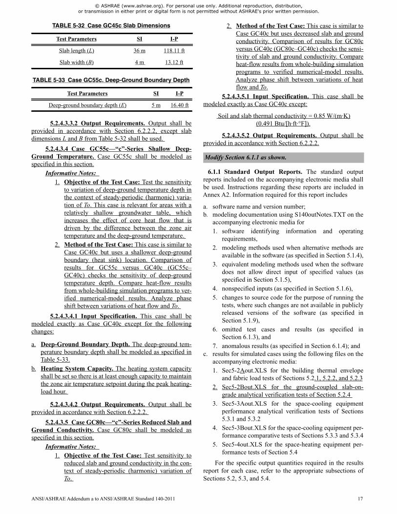
© ASHRAE (www.ashrae.org). For personal use only. Additional reproduction, distribution, or transmission in either print or digital form is not permitted without ASHRAE's prior written permission.
5.2.4.3.3.2 Output Requirements. Output shall beprovided in accordance with Section 6.2.2.2, except slabdimensions L and B from Table 5-32 shall be used.
5.2.4.3.4 Case GC55c—“c”-Series Shallow Deep-Ground Temperature. Case GC55c shall be modeled asspecified in this section.
Informative Notes:1. Objective of the Test Case: Test the sensitivity
to variation of deep-ground temperature depth inthe context of steady-periodic (harmonic) varia-tion of To. This case is relevant for areas with arelatively shallow groundwater table, whichincreases the effect of core heat flow that isdriven by the difference between the zone airtemperature and the deep-ground temperature.
2. Method of the Test Case: This case is similar toCase GC40c but uses a shallower deep-groundboundary (heat sink) location. Comparison ofresults for GC55c versus GC40c (GC55c–GC40c) checks the sensitivity of deep-groundtemperature depth. Compare heat-flow resultsfrom whole-building simulation programs to ver-ified numerical-model results. Analyze phaseshift between variations of heat flow and To.
5.2.4.3.4.1 Input Specification. This case shall bemodeled exactly as Case GC40c except for the followingchanges:
a. Deep-Ground Boundary Depth. The deep-ground tem-perature boundary depth shall be modeled as specified inTable 5-33.
b. Heating System Capacity. The heating system capacityshall be set so there is at least enough capacity to maintainthe zone air temperature setpoint during the peak heating-load hour.
5.2.4.3.4.2 Output Requirements. Output shall beprovided in accordance with Section 6.2.2.2.
5.2.4.3.5 Case GC80c—“c”-Series Reduced Slab andGround Conductivity. Case GC80c shall be modeled asspecified in this section.
Informative Notes:1. Objective of the Test Case: Test sensitivity to
reduced slab and ground conductivity in the con-text of steady-periodic (harmonic) variation ofTo.
2. Method of the Test Case: This case is similar toCase GC40c but uses decreased slab and groundconductivity. Comparison of results for GC80cversus GC40c (GC80c–GC40c) checks the sensi-tivity of slab and ground conductivity. Compareheat-flow results from whole-building simulationprograms to verified numerical-model results.Analyze phase shift between variations of heatflow and To.
5.2.4.3.5.1 Input Specification. This case shall bemodeled exactly as Case GC40c except:
Soil and slab thermal conductivity = 0.85 W/(m·K)(0.491 Btu/[h·ft·°F]).
5.2.4.3.5.2 Output Requirements. Output shall beprovided in accordance with Section 6.2.2.2.
6.1.1 Standard Output Reports. The standard outputreports included on the accompanying electronic media shallbe used. Instructions regarding these reports are included inAnnex A2. Information required for this report includes
a. software name and version number;b. modeling documentation using S140outNotes.TXT on the
accompanying electronic media for1. software identifying information and operating
requirements,2. modeling methods used when alternative methods are
available in the software (as specified in Section 5.1.4),3. equivalent modeling methods used when the software
does not allow direct input of specified values (asspecified in Section 5.1.5),
4. nonspecified inputs (as specified in Section 5.1.6),5. changes to source code for the purpose of running the
tests, where such changes are not available in publiclyreleased versions of the software (as specified inSection 5.1.9),
6. omitted test cases and results (as specified inSection 6.1.3), and
7. anomalous results (as specified in Section 6.1.4); andc. results for simulated cases using the following files on the
accompanying electronic media:1. Sec5-2Aout.XLS for the building thermal envelope
and fabric load tests of Sections 5.2.1, 5.2.2, and 5.2.32. Sec5-2Bout.XLS for the ground-coupled slab-on-
grade analytical verification tests of Section 5.2.43. Sec5-3Aout.XLS for the space-cooling equipment
performance analytical verification tests of Sections5.3.1 and 5.3.2
4. Sec5-3Bout.XLS for the space-cooling equipment per-formance comparative tests of Sections 5.3.3 and 5.3.4
5. Sec5-4out.XLS for the space-heating equipment per-formance tests of Section 5.4
For the specific output quantities required in the resultsreport for each case, refer to the appropriate subsections ofSections 5.2, 5.3, and 5.4.
TABLE 5-32 Case GC45c Slab Dimensions
Test Parameters SI I-P
Slab length (L) 36 m 118.11 ft
Slab width (B) 4 m 13.12 ft
TABLE 5-33 Case GC55c. Deep-Ground Boundary Depth
Test Parameters SI I-P
Deep-ground boundary depth (E) 5 m 16.40 ft
Modify Section 6.1.1 as shown.
ANSI/ASHRAE Addendum a to ANSI/ASHRAE Standard 140-2011 17
© ASHRAE (www.ashrae.org). For personal use only. Additional reproduction, distribution, or transmission in either print or digital form is not permitted without ASHRAE's prior written permission.
6.2 Output Requirements for Building Thermal Envelopeand Fabric Load and Ground-Coupled Slab-on-GradeTests of Section 5.2. Required output shall be as specified inthe sections below.
6.2.1 Output Requirements for Building Thermal Enve-lope and Fabric Load Tests of Sections 5.2.1, 5.2.2, and5.2.36.2.1.1 All Non-Free-Float Cases. Required outputs for thenon-free-float cases shall be as designated in Sections6.2.1.1.1 through 6.2.1.1.5:
Informative Note: In this description, the term “free-floatcases” refers to cases designated with FF in the case descrip-tion (i.e., 600FF, 650FF, 900FF, 950FF); non-free-float casesare all the other cases described in Sections 5.2.1, 5.2.2, and5.2.3 (Tables B1-1a and B1-1b of Annex B1 include an infor-mative summary listing of the cases of Sections 5.2.1, 5.2.2,and 5.2.3).
6.2.1.1.1 Annual heating load (MWh).6.2.1.1.2 Annual sensible cooling loads (MWh).6.2.1.1.3 Annual hourly integrated peak heating load
(kW) with date and hour of occurrence.6.2.1.1.4 Annual hourly integrated peak sensible cooling
load (kW) with date and hour of occurrence.6.2.1.1.5 All heating and cooling loads listed in Sections
6.2.1.1.1 through 6.2.1.1.4 shall be entered into the appropri-ate standard output report (as specified in Annex A2) as posi-tive values (0).
6.2.1.2 Case 600 Only6.2.1.2.1 Annual incident unshaded total solar radiation
(diffuse and direct) on north, east, west, south, and horizontalsurfaces (kWh/m2).
6.2.1.2.2 Unshaded annual transmitted solar radiation(diffuse and direct) through south windows (kWh/m2). Thisquantity does not include radiation that is absorbed in theglass and conducted inward as heat.
Informative Note: This quantity may be taken as theoptically transmitted solar radiation through a window that isbacked by a perfectly absorbing black cavity.
6.2.1.3 Case 610 Only6.2.1.3.1 Annual transmitted solar radiation through the
shaded south window with a horizontal overhang (kWh/m2).6.2.1.4 Case 620 Only
6.2.1.4.1 Unshaded annual transmitted solar radiation(diffuse and direct) through the west window (kWh/m2). Thisquantity does not include radiation that is absorbed in theglass and conducted inward as heat.
Informative Note: This quantity may be taken as theoptically transmitted solar radiation through a window that isbacked by a perfectly absorbing black cavity.
6.2.1.5 Case 630 Only
6.2.1.5.1 Annual transmitted solar radiation through theshaded west window with horizontal overhang and verticalfins (kWh/m2).
6.2.1.6 All Free-Float Cases. Required outputs for thefree-float cases shall be as designated in Sections 6.2.1.6.1through 6.2.1.6.3.
Informative Note: Informative Note: In this description,the term “free-float cases” refers to cases designated with FFin the case description (i.e., 600FF, 650FF, 900FF, 950FF, andfor just the sun zone in Case 960).
6.2.1.6.1 Annual hourly integrated maximum zone airtemperature, °C, with date and hour of occurrence.
6.2.1.6.2 Annual hourly integrated minimum zone airtemperature, °C, with date and hour of occurrence.
6.2.1.6.3 Annual mean zone air temperature, °C.Informative Note: For all cases where free-float-zone air
temperature output is required, the free-float-zone air temper-ature is for the zone air only, assuming well-mixed air with noradiant effects (i.e., equivalent to what would be obtainedfrom an aspirated temperature sensor perfectly shielded fromsolar and infrared radiation).
6.2.1.7 Case 900FF Only6.2.1.7.1 Annual hourly 1°C zone air temperature bin fre-
quencies from –20°C to 70°C, where “bin frequency” is thenumber of hours a given zone air temperature has valueswithin given bins (1°C bin width) during the annual simula-tion. Zone air temperature bins are defined by an integer valueof temperature as the lower bound (inclusive) of the range, theupper bound of the range being less than the next highest inte-ger value.
Informative Note: For example, the zone air temperature(T) bin defined by 20°C is 20°C T 21°C; and similarly thebin defined by –2°C is –2°C T –1°C.
Output Example: Output from an annual simulation(8760 hours) might indicate 400 hours when the zone air tem-perature (T) is 25°C (25°C T < 26°C) and 430 hours whenthe zone air temperature is 28°C (28°C T < 29°C), withtemperatures for remaining hours distributed among otherbins as appropriate.
Additional information regarding this calculation is pro-vided in Informative Annex B12.
6.2.1.8 Daily Hourly Output for Building ThermalEnvelope and Fabric Load Tests of Sections 5.2.1 and5.2.2. If the program being tested is capable of producinghourly outputs, then the following hourly values for the speci-fied days shall be provided. To produce this output, the simu-lation period shall be a typical annual run, as specified inSections 5.1.7 and 5.1.8.1.
Running the simulation for only the required days speci-fied in the output requirements shall be prohibited, becausethe results could contain temperature history errors. Requiredoutputs shall be as listed for specific cases in Table 6-1.
TABLE 6-1 Daily Hourly Output Requirements forBuilding Thermal Envelope and Fabric Load Tests of
Sections 5.2.1 and 5.2.2
Insert new subsection 6.2.1 for existing Envelope and Fab-ric Load Test and renumber existing subsections ofSection 6.2 (6.2.n) as subsections of 6.2.1(6.2.1.n). All refer-ences to Section 6.2 and its subsections (6.2.n) inStandard 140-2011 will be changed to referenceSection 6.2.1 and its subsections (6.2.1.n).
Revise title of Table 6-1 as shown.
18 ANSI/ASHRAE Addendum a to ANSI/ASHRAE Standard 140-2011
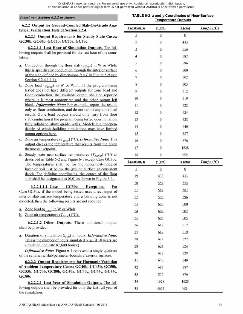
© ASHRAE (www.ashrae.org). For personal use only. Additional reproduction, distribution, or transmission in either print or digital form is not permitted without ASHRAE's prior written permission.
6.2.2 Output for Ground-Coupled Slab-On-Grade Ana-lytical Verification Tests of Section 5.2.4
6.2.2.1 Output Requirements for Steady State Cases:GC30b, GC60b, GC65b, GC30a, GC30c
6.2.2.1.1 Last Hour of Simulation Outputs. The fol-lowing outputs shall be provided for the last hour of the simu-lation:
a. Conduction through the floor slab (qfloor) in W or Wh/h;this is specifically conduction through the interior surfaceof the slab defined by dimensions B × L in Figure 5-9 (seeSection 5.2.4.1.1.1).
b. Zone load (qzone) in W or Wh/h. If the program beingtested does not have different outputs for zone load andfloor conduction, the available output shall be reportedwhere it is most appropriate and the other output leftblank. Informative Note: For example, report the resultsonly as floor conduction, and do not report any zone loadresults. Zone load outputs should only vary from floorslab conduction if the program being tested does not allowfully adiabatic above-grade walls. Models run indepen-dently of whole-building simulations may have limitedoutput options here.
c. Zone air temperature (Tzone) (°C). Informative Note: Thisoutput checks the temperature that results from the giventhermostat setpoint.
d. Steady state near-surface temperatures (Tsurf,n) (°C) asdescribed in Table 6-2 and Figure 6-1 except Case GC30c.The temperatures shall be for the uppermost-modeledlayer of soil just below the ground surface at consistentdepth. For defining coordinates, the center of the floorslab shall be designated as (0,0) as shown in Figure 6-1.
6.2.2.1.1.1 Case GC30a Exception. ForCase GC30a, if the model being tested uses direct input ofinterior slab surface temperature and a building zone is notmodeled, then the following results are not required:
a. Zone load (qzone) in W or Wh/hb. Zone air temperature (Tzone) (°C).
6.2.2.1.2 Other Outputs. These additional outputsshall be provided:
a. Duration of simulation (tsim) in hours. Informative Note:This is the number of hours simulated (e.g., if 10 years aresimulated, indicate 87,600 hours.)Informative Note: Figure 6-1 represents a single quadrant
of the symmetric slab/perimeter-boundary/exterior surfaces.
6.2.2.2 Output Requirements for Harmonic Variationof Ambient Temperature Cases: GC40b, GC45b, GC50b,GC55b, GC70b, GC80b, GC40a, GC40c, GC45c, GC55c,GC80c
6.2.2.2.1 Last Year of Simulation Outputs. The fol-lowing outputs shall be provided for only the last full year ofthe simulation:
Insert new Section 6.2.2 as shown. TABLE 6-2 x and y Coordinates of Near-SurfaceTemperature Outputs
Location, n y (cm) x (cm) Tsurf,n (°C)
1 0 0
2 0 433
3 0 554
4 0 587
5 0 596
6 0 600
7 0 602
8 0 605
9 0 612
10 0 619
11 0 622
12 0 624
13 0 628
14 0 640
15 0 687
16 0 876
17 0 1628
18 0 4624
Location, n y (cm) x (cm) Tsurf,n (°C)
1 0 0
19 433 433
20 554 554
21 587 587
22 596 596
23 600 600
24 602 602
25 605 605
26 612 612
27 619 619
28 622 622
29 624 624
30 628 628
31 640 640
32 687 687
33 876 876
34 1628 1628
35 4624 4624
ANSI/ASHRAE Addendum a to ANSI/ASHRAE Standard 140-2011 19
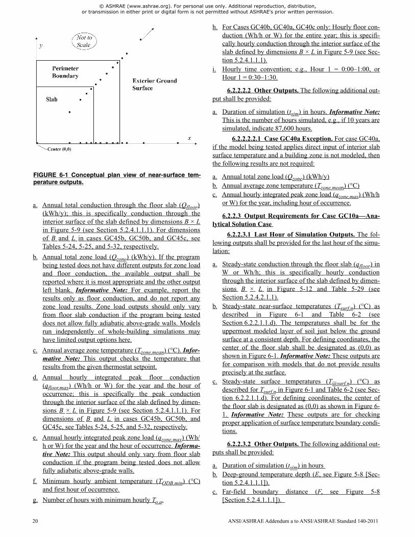
© ASHRAE (www.ashrae.org). For personal use only. Additional reproduction, distribution, or transmission in either print or digital form is not permitted without ASHRAE's prior written permission.
a. Annual total conduction through the floor slab (Qfloor)(kWh/y); this is specifically conduction through theinterior surface of the slab defined by dimensions B × Lin Figure 5-9 (see Section 5.2.4.1.1.1). For dimensionsof B and L in cases GC45b, GC50b, and GC45c, seeTables 5-24, 5-25, and 5-32, respectively.
b. Annual total zone load (Qzone) (kWh/y). If the programbeing tested does not have different outputs for zone loadand floor conduction, the available output shall bereported where it is most appropriate and the other outputleft blank. Informative Note: For example, report theresults only as floor conduction, and do not report anyzone load results. Zone load outputs should only varyfrom floor slab conduction if the program being testeddoes not allow fully adiabatic above-grade walls. Modelsrun independently of whole-building simulations mayhave limited output options here.
c. Annual average zone temperature (Tzone,mean) (°C). Infor-mative Note: This output checks the temperature thatresults from the given thermostat setpoint.
d. Annual hourly integrated peak floor conduction(qfloor,max) (Wh/h or W) for the year and the hour ofoccurrence; this is specifically the peak conductionthrough the interior surface of the slab defined by dimen-sions B × L in Figure 5-9 (see Section 5.2.4.1.1.1). Fordimensions of B and L in cases GC45b, GC50b, andGC45c, see Tables 5-24, 5-25, and 5-32, respectively.
e. Annual hourly integrated peak zone load (qzone,max) (Wh/h or W) for the year and the hour of occurrence. Informa-tive Note: This output should only vary from floor slabconduction if the program being tested does not allowfully adiabatic above-grade walls.
f. Minimum hourly ambient temperature (TODB,min) (°C)and first hour of occurrence.
g. Number of hours with minimum hourly To,a.
h. For Cases GC40b, GC40a, GC40c only: Hourly floor con-duction (Wh/h or W) for the entire year; this is specifi-cally hourly conduction through the interior surface of theslab defined by dimensions B × L in Figure 5-9 (see Sec-tion 5.2.4.1.1.1).
i. Hourly time convention; e.g., Hour 1 = 0:00–1:00, orHour 1 = 0:30–1:30.
6.2.2.2.2 Other Outputs. The following additional out-put shall be provided:
a. Duration of simulation (tsim) in hours. Informative Note:This is the number of hours simulated, e.g., if 10 years aresimulated, indicate 87,600 hours.
6.2.2.2.2.1 Case GC40a Exception. For case GC40a,if the model being tested applies direct input of interior slabsurface temperature and a building zone is not modeled, thenthe following results are not required:
a. Annual total zone load (Qzone) (kWh/y)b. Annual average zone temperature (Tzone,mean) (°C)c. Annual hourly integrated peak zone load (qzone,max) (Wh/h
or W) for the year, including hour of occurrence.
6.2.2.3 Output Requirements for Case GC10a—Ana-lytical Solution Case
6.2.2.3.1 Last Hour of Simulation Outputs. The fol-lowing outputs shall be provided for the last hour of the simu-lation:
a. Steady-state conduction through the floor slab (qfloor) inW or Wh/h; this is specifically hourly conductionthrough the interior surface of the slab defined by dimen-sions B × L in Figure 5-12 and Table 5-29 (seeSection 5.2.4.2.1.1).
b. Steady-state near-surface temperatures (Tsurf,n) (°C) asdescribed in Figure 6-1 and Table 6-2 (seeSection 6.2.2.1.1.d). The temperatures shall be for theuppermost modeled layer of soil just below the groundsurface at a consistent depth. For defining coordinates, thecenter of the floor slab shall be designated as (0,0) asshown in Figure 6-1. Informative Note: These outputs arefor comparison with models that do not provide resultsprecisely at the surface.
c. Steady-state surface temperatures (T@surf,n) (°C) asdescribed for Tsurf,n in Figure 6-1 and Table 6-2 (see Sec-tion 6.2.2.1.1.d). For defining coordinates, the center ofthe floor slab is designated as (0,0) as shown in Figure 6-1. Informative Note: These outputs are for checkingproper application of surface temperature boundary condi-tions.
6.2.2.3.2 Other Outputs. The following additional out-puts shall be provided:
a. Duration of simulation (tsim) in hoursb. Deep-ground temperature depth (E, see Figure 5-8 [Sec-
tion 5.2.4.1.1.1]).c. Far-field boundary distance (F, see Figure 5-8
[Section 5.2.4.1.1.1]).
FIGURE 6-1 Conceptual plan view of near-surface tem-perature outputs.
20 ANSI/ASHRAE Addendum a to ANSI/ASHRAE Standard 140-2011
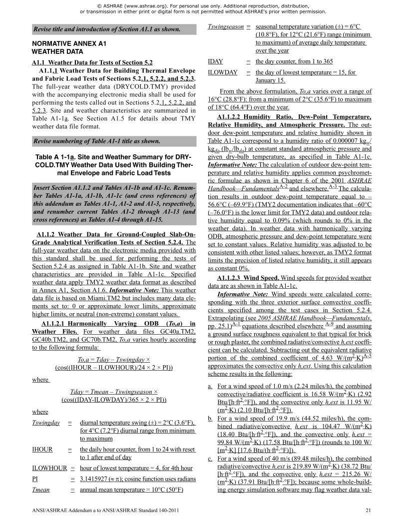
© ASHRAE (www.ashrae.org). For personal use only. Additional reproduction, distribution, or transmission in either print or digital form is not permitted without ASHRAE's prior written permission.
NORMATIVE ANNEX A1WEATHER DATA
A1.1 Weather Data for Tests of Section 5.2A1.1.1 Weather Data for Building Thermal Envelope
and Fabric Load Tests of Sections 5.2.1, 5.2.2, and 5.2.3.The full-year weather data (DRYCOLD.TMY) providedwith the accompanying electronic media shall be used forperforming the tests called out in Sections 5.2.1, 5.2.2, and5.2.3. Site and weather characteristics are summarized inTable A1-1a. See Section A1.5 for details about TMYweather data file format.
Table A 1-1a. Site and Weather Summary for DRY-COLD.TMY Weather Data Used With Building Ther-
mal Envelope and Fabric Load Tests
A1.1.2 Weather Data for Ground-Coupled Slab-On-Grade Analytical Verification Tests of Section 5.2.4. Thefull-year weather data on the electronic media provided withthis standard shall be used for performing the tests ofSection 5.2.4 as assigned in Table A1-1b. Site and weathercharacteristics are provided in Table A1-1c. Specifiedweather data apply TMY2 weather data format as describedin Annex A1, Section A1.6. Informative Note: This weatherdata file is based on Miami.TM2 but includes many data ele-ments set to: 0 or approximate lower limits, approximatehigher limits, or neutral (non-extreme) constant values.
A1.1.2.1 Harmonically Varying ODB (To,a) inWeather Files. For weather data files GC40a.TM2,GC40b.TM2, and GC70b.TM2, To,a varies hourly accordingto the following formula:
To,a = Tday – Tswingday ×(cos((IHOUR – ILOWHOUR)/24 × 2 × PI))
where
Tday = Tmean – Tswingseason ×(cos((IDAY-ILOWDAY)/365 × 2 × PI))
where
Tswingday = diurnal temperature swing (±) = 2°C (3.6°F),for 4°C (7.2°F) diurnal range from minimumto maximum
IHOUR = the daily hour counter, from 1 to 24 with resetto 1 after end of day
ILOWHOUR = hour of lowest temperature = 4, for 4th hour
PI = 3.1415927 ( ); cosine function uses radians
Tmean = annual mean temperature = 10°C (50°F)
Tswingseason = seasonal temperature variation (±) = 6°C(10.8°F), for 12°C (21.6°F) range (minimumto maximum) of average daily temperatureover the year
IDAY = the day counter, from 1 to 365
ILOWDAY = the day of lowest temperature = 15, forJanuary 15.
From the above formulation, To,a varies over a range of16°C (28.8°F): from a minimum of 2°C (35.6°F) to maximumof 18°C (64.4°F) over the year.
A1.1.2.2 Humidity Ratio, Dew-Point Temperature,Relative Humidity, and Atmospheric Pressure. The out-door dew-point temperature and relative humidity shown inTable A1-1c correspond to a humidity ratio of 0.000007 kgw/kgda (lbw/lbda) at constant standard atmospheric pressure andgiven dry-bulb temperature, as specified in Table A1-1c.Informative Note: The calculation of outdoor dew-point tem-perature and relative humidity applies common psychromet-ric formulae as shown in Chapter 6 of the 2001 ASHRAEHandbook—FundamentalsA-2 and elsewhere.A-3 The calcula-tion results in outdoor dew-point temperature equal to –56.6°C (–69.9°F) (TMY2 documentation indicates that –60°C(–76.0°F) is the lower limit for TMY2 data) and outdoor rela-tive humidity equal to 0.09% (which rounds to 0% in theweather data). In weather data with harmonically varyingODB, atmospheric pressure and dew-point temperature wereset to constant values. Relative humidity was adjusted to beconsistent with other listed values; however, as TMY2 formatlimits the precision of listed relative humidity, it still appearsas constant 0%.
A1.1.2.3 Wind Speed. Wind speeds for provided weatherdata are as shown in Table A1-1c.
Informative Note: Wind speeds were calculated corre-sponding with the three exterior surface convective coeffi-cients specified among the test cases in Section 5.2.4.Extrapolating (see 2005 ASHRAE Handbook—Fundamentals,pp. 25.1)A-1 equations described elsewhere A-9 and assuminga ground surface roughness equivalent to that typical for brickor rough plaster, the combined radiative/convective h,ext coeffi-cient can be calculated. Subtracting out the equivalent radiativeportion of the combined coefficient of 4.63 W/(m2·K)A-5
approximates the convective only h,ext. Using this calculationscheme results in the following:
a. For a wind speed of 1.0 m/s (2.24 miles/h), the combinedconvective/radiative coefficient is 16.58 W/(m2·K) (2.92Btu/[h·ft2·°F]), and the convective only h,ext is 11.95 W/(m2·K) (2.10 Btu/[h·ft2·°F]).
b. For a wind speed of 19.9 m/s (44.52 miles/h), the com-bined radiative/convective h,ext is 104.47 W/(m2·K)(18.40 Btu/[h·ft2·°F]), and the convective only h,ext =99.84 W/(m2·K) (17.58 Btu/[h·ft2·°F]) (rounds to 100 W/[m2·K] [17.6 Btu/(h·ft2·°F)]).
c. For a wind speed of 40 m/s (89.48 miles/h), the combinedradiative/convective h,ext is 219.89 W/(m2·K) (38.72 Btu/[h·ft2·°F]), and the convective only h,ext = 215.26 W/(m2·K) (37.91 Btu/[h·ft2·°F]); because some whole-build-ing energy simulation software may flag weather data val-
Revise title and introduction of Section A1.1 as shown.
Revise numbering of Table A1-1 title as shown.
Insert Section A1.1.2 and Tables A1-1b and A1-1c. Renum-ber Tables A1-1a, A1-1b, A1-1c (and cross references) ofthis addendum as Tables A1-1, A1-2 and A1-3, respectively,and renumber current Tables A1-2 through A1-13 (andcross references) as Tables A1-4 through A1-15.
ANSI/ASHRAE Addendum a to ANSI/ASHRAE Standard 140-2011 21
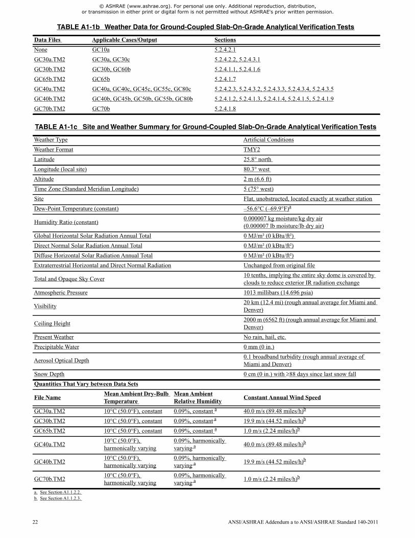
© ASHRAE (www.ashrae.org). For personal use only. Additional reproduction, distribution, or transmission in either print or digital form is not permitted without ASHRAE's prior written permission.
TABLE A1-1b Weather Data for Ground-Coupled Slab-On-Grade Analytical Verification Tests
Data Files Applicable Cases/Output Sections
None GC10a 5.2.4.2.1
GC30a.TM2 GC30a, GC30c 5.2.4.2.2, 5.2.4.3.1
GC30b.TM2 GC30b, GC60b 5.2.4.1.1, 5.2.4.1.6
GC65b.TM2 GC65b 5.2.4.1.7
GC40a.TM2 GC40a, GC40c, GC45c, GC55c, GC80c 5.2.4.2.3, 5.2.4.3.2, 5.2.4.3.3, 5.2.4.3.4, 5.2.4.3.5
GC40b.TM2 GC40b, GC45b, GC50b, GC55b, GC80b 5.2.4.1.2, 5.2.4.1.3, 5.2.4.1.4, 5.2.4.1.5, 5.2.4.1.9
GC70b.TM2 GC70b 5.2.4.1.8
TABLE A1-1c Site and Weather Summary for Ground-Coupled Slab-On-Grade Analytical Verification Tests
Weather Type Artificial Conditions
Weather Format TMY2
Latitude 25.8° north
Longitude (local site) 80.3° west
Altitude 2 m (6.6 ft)
Time Zone (Standard Meridian Longitude) 5 (75° west)
Site Flat, unobstructed, located exactly at weather station
Dew-Point Temperature (constant) –56.6°C (–69.9°F)a
Humidity Ratio (constant)0.000007 kg moisture/kg dry air(0.000007 lb moisture/lb dry air)
Global Horizontal Solar Radiation Annual Total 0 MJ/m² (0 kBtu/ft²)
Direct Normal Solar Radiation Annual Total 0 MJ/m² (0 kBtu/ft²)
Diffuse Horizontal Solar Radiation Annual Total 0 MJ/m² (0 kBtu/ft²)
Extraterrestrial Horizontal and Direct Normal Radiation Unchanged from original file
Total and Opaque Sky Cover10 tenths, implying the entire sky dome is covered byclouds to reduce exterior IR radiation exchange
Atmospheric Pressure 1013 millibars (14.696 psia)
Visibility20 km (12.4 mi) (rough annual average for Miami andDenver)
Ceiling Height2000 m (6562 ft) (rough annual average for Miami andDenver)
Present Weather No rain, hail, etc.
Precipitable Water 0 mm (0 in.)
Aerosol Optical Depth0.1 broadband turbidity (rough annual average ofMiami and Denver)
Snow Depth 0 cm (0 in.) with 88 days since last snow fall
Quantities That Vary between Data Sets
File NameMean Ambient Dry-BulbTemperature
Mean AmbientRelative Humidity
Constant Annual Wind Speed
GC30a.TM2 10°C (50.0°F), constant 0.09%, constant a 40.0 m/s (89.48 miles/h)b
GC30b.TM2 10°C (50.0°F), constant 0.09%, constant a 19.9 m/s (44.52 miles/h)b
GC65b.TM2 10°C (50.0°F), constant 0.09%, constant a 1.0 m/s (2.24 miles/h)b
GC40a.TM210°C (50.0°F),harmonically varying
0.09%, harmonicallyvarying a 40.0 m/s (89.48 miles/h)b
GC40b.TM210°C (50.0°F),harmonically varying
0.09%, harmonicallyvarying a 19.9 m/s (44.52 miles/h)b
GC70b.TM210°C (50.0°F),harmonically varying
0.09%, harmonicallyvarying a 1.0 m/s (2.24 miles/h)b
a. See Section A1.1.2.2.b. See Section A1.1.2.3.
22 ANSI/ASHRAE Addendum a to ANSI/ASHRAE Standard 140-2011
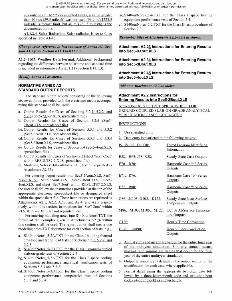
© ASHRAE (www.ashrae.org). For personal use only. Additional reproduction, distribution, or transmission in either print or digital form is not permitted without ASHRAE's prior written permission.
ues outside of TMY2 documented limits, a value greaterthan 40 m/s (89.5 miles/h) was not used (99.9 m/s [223.5miles/h] is format limit, but 40 m/s (89.5 miles/h) is thedocumented limit).A1.1.2.4 Solar Radiation. Solar radiation is set to 0, as
specified in Table A1-1c.
A1.5 TMY Weather Data Format. Additional backgroundregarding the difference between solar time and standard timeis included in informative Annex B11 (Section B11.1.3).
NORMATIVE ANNEX A2STANDARD OUTPUT REPORTS
The standard output reports consisting of the followingsix seven forms provided with the electronic media accompa-nying this standard shall be used:
a. Output Results for Cases of Sections 5.2.1, 5.2.2, and5.2.3 (Sec5-2Aout.XLS, spreadsheet file)
b. Output Results for Cases of Section 5.2.4 (Sec5-2Bout.XLS, spreadsheet file)
bc. Output Results for Cases of Sections 5.3.1 and 5.3.2(Sec5-3Aout.XLS, spreadsheet file)
cd. Output Results for Cases of Sections 5.3.3 and 5.3.4(Sec5-3Bout.XLS, spreadsheet file)
de. Output Results for Cases of Section 5.4 (Sec5-4out.XLS,spreadsheet file)
ef. Output Results for Cases of Section 7.2 (sheet ‘Sec7-2out’within RESULTS7-2.XLS spreadsheet file)
fg. Modeling Notes (S140outNotes.TXT, text file reprinted asAttachment A2.65)
For entering output results into Sec5-2Aout.XLS, Sec5-2Bout.XLS, Sec5-3Aout.XLS, Sec5-3Bout.XLS, Sec5-4out.XLS, and sheet ‘Sec7-2out’ within RESULTS7-2.XLS,the user shall follow the instructions provided at the top of theappropriate electronic spreadsheet file or designated sheetwithin the spreadsheet file. These instructions are reprinted asAttachments A2.1, A2.2, A2.3, and A2.4, and A2.5 respec-tively, within this section; instructions for ‘Sec7-2out’ withinRESULTS7-2.XLS are not reprinted here.
For entering modeling notes into S140outNotes.TXT, theformat of the examples given in Attachments A2.76 withinthis section shall be used. The report author shall create onemodeling notes TXT document for each section of tests; e.g.,
a. S140outNotes_5-2A.TXT for the Class I building thermalenvelope and fabric load tests of Sections 5.2.1, 5.2.2, and5.2.3
b. S140outNotes_5-2B.TXT for the Class I ground-coupledslab-on-grade tests of Section 5.2.4
bc. S140outNotes_5-3A.TXT for the Class I space coolingequipment performance analytical verification tests ofSections 5.3.1 and 5.3.2
cd. S140outNotes_5-3B.TXT for the Class I space coolingequipment performance comparative tests of Sections5.3.3 and 5.3.4
.de.S140outNotes_5-4.TXT for the Class I space heatingequipment performance tests of Section 5.4.
ef. S140outNotes_7-2.TXT for the Class II test procedures ofSection 7.2.
Attachment A2.23 Instructions for Entering Resultsinto Sec5-3Aout.XLS
Attachment A2.34 Instructions for Entering Resultsinto Sec5-3Bout.XLS
Attachment A2.45 Instructions for Entering Resultsinto Sec5-4out.XLS
Attachment A2.2 Instructions forEntering Results into Sec5-2Bout.XLS
Sec5-2Bout.XLS OUTPUT SPREADSHEET FORGROUND-COUPLED SLAB-ON-GRADE ANALYTICALVERIFICATION CASES: GC10a-GC80c
INSTRUCTIONS
1. Use specified units
2. Data entry is restricted to the following ranges:
I5...I8; O5...O6; O8: Tested Program IdentifyingInformation
E58…H63; J58, K58: Steady-State Case Outputs
E70…R70: Harmonic Case “a”-SeriesOutputs
E71…R76: Harmonic Case “b”-SeriesOutputs
E77…R80: Harmonic Case “c”-SeriesOutputs
G86…K103; G105…K122: Steady-State Near-SurfaceTemperature Outputs
M86…M103; M105…M122: GC10a At-Surface Tempera-ture Outputs
G126: Hourly Time Convention
E131…G8890: Hourly Floor ConductionOutputs
3. Annual sums and means are values for the entire final yearof the multiyear simulation. Similarly, annual means,maxima, and minima are values that occur for the finalyear of the entire multiyear simulation.
4. Output terminology is defined in the output section of thespecification for each case, where applicable.
5. Format dates using the appropriate two-digit date fol-lowed by a three-letter month code and two-digit hourcode (24-hour clock) as shown below.
Change cross reference in last sentence of Annex A1, Sec-tion A1.5 from Section B11.3 to B11.1.3.
Modify Annex A2 as shown.
Renumber titles of Attachments A2.2–A2.4 as shown.
Add new Attachment A2.2 as shown.
ANSI/ASHRAE Addendum a to ANSI/ASHRAE Standard 140-2011 23
© ASHRAE (www.ashrae.org). For personal use only. Additional reproduction, distribution, or transmission in either print or digital form is not permitted without ASHRAE's prior written permission.
For example, a maximum value occurring on August 16during the 15th hour interval (2:00 p.m. to 3:00 p.m.), shall beinput as:
Attachment A2.56—Standard 140 Output Form(S140outNotes.TXT)—Modeling Notes
MODELING NOTES FOR ASHRAE STANDARD 140INTRODUCTION
This document shall include supplemental informationabout the ASHRAE Standard 140 tests performed. OneS140outNotes document shall be provided for each set oftests (e.g., one for the building thermal and fabric load tests ofSections 5.2.1, 5.2.2, and 5.2.3; one for the space coolingequipment analytical verification tests of Sections 5.3.1 and5.3.2; etc.) [ . . . ]
INFORMATIVE ATTACHMENT A2.67—EXAMPLESOF MODELING NOTES
MODELING NOTES FORASHRAE STANDARD 140—EXAMPLES
OVERVIEW
This document contains examples of modeling notesentered in the S140outNotes_Sec5-x.TXT file. Examples areprovided to guide in filling out the S140outNotes_Sec5-x.TXT file.
Note that in this file, sample notes refer to different sec-tions of Standard 140. In an actual S140outNotes_Sec5-x.TXT file the notes would only address one set of testswithin Standard 140 (e.g., the building thermal and fabricload tests of Sections 5.2.1, 5.2.2, and 5.2.3).
INTRODUCTION
This document shall include supplemental informationabout the ASHRAE Standard 140 tests performed. OneS140outNotes document shall be provided for each set oftests (e.g., one for the building thermal and fabric loadtests of Sections 5.2.1, 5.2.2, and 5.2.3; one for the spacecooling equipment analytical verification tests ofSections 5.3.1 and 5.3.2; etc.)
B. REPORT BLOCK FORALTERNATIVE MODELING METHODS
[ . . . ]
Note 1: Convective Heat Transfer and RadiativeExchange Related to Both Interior and Exterior Surfaces(Sections 5-2 5.2.1, 5.2.2, and 5.2.3)
[ . . . ]
Note 2: Interior Transmitted Solar Radiation Distribution(Sections5-2 5.2.1, 5.2.2, and 5.2.3)
[ . . . ]
Note 3: Thermal Behavior of Windows (Sections 5-25.2.1, 5.2.2, and 5.2.3)
[ . . . ]
C. REPORT BLOCK FOREQUIVALENT MODELING METHODS
[ . . . ]
Note 1: Thermal Decoupling of Floor from Ground (Sec-tion 5-2 5.2.1)
[ . . . ]
Note 2: Thermostat Control and Equipment Capacity(Section 5-2 5.2.1)
[ . . . ]
E. REPORT BLOCK FOROMITTED TEST CASES AND RESULTS
[ . . . ]
MONTH CODE
JANUARY Jan
FEBRUARY Feb
MARCH Mar
APRIL Apr
MAY May
JUNE Jun
JULY Jul
AUGUST Aug
SEPTEMBER Sep
OCTOBER Oct
NOVEMBER Nov
DECEMBER Dec
Date Hour
16-Aug 15
Renumber title of normative Attachment A2.5, and revise asshown. S140outNotes.TXT is updated as shown. Theupdated version of this file is included with \Sec5-2AFiles\Normative Materials and \Sec5-2BFiles\NormativeMaterials files and will replace the current file in the otherSec5-n\Normative Materials files.
Renumber title of informative Attachment A2.6, andrevise as shown. S140outNotes_Examples.TXT isupdated as shown. The updated version of this file isincluded with \Sec5-2AFiles\Informative Materials and\Sec5-2BFiles\Informative Materials files and willreplace the current file in the other Sec5-n\InformativeMaterials files
24 ANSI/ASHRAE Addendum a to ANSI/ASHRAE Standard 140-2011
© ASHRAE (www.ashrae.org). For personal use only. Additional reproduction, distribution, or transmission in either print or digital form is not permitted without ASHRAE's prior written permission.
Note 1: Light Weight Test Cases (Sections 5-2 5.2.1,5.2.2, and 5.2.3)
[ . . . ]
Note 2: Case 960- Sunspace, All Results (Section 5-25.2.2)
[ . . . ]
INFORMATIVE ANNEX B1TABULAR SUMMARY OF TEST CASES
Tables B1-1a and B1-1b include a tabular summary ofthe Class I building thermal envelope and fabric load testcases described in Sections 5.2.1, 5.2.2, and 5.2.3, in SIunits only. Tables B1-1c and B1-1d include a tabular sum-mary of the Class I ground-coupled slab-on-grade analyti-cal verification test cases described in Section 5.2.4, in SIunits only. Tables B1-2a and B1-2b include a tabular sum-mary of the Space-Cooling Equipment Performance Ana-lytical Verification Test Cases described in Sections 5.3.1and 5.3.2, in SI and I-P units, respectively. Table B1-3includes a tabular summary of the Space-Cooling Equip-ment Performance Comparative Test Cases described inSections 5.3.3 and 5.3.4, in SI units only. Table B1-4 sum-marizes the Space-Heating Equipment test cases describedin Section 5.4, in SI units only. Table B1-5 summarizes theClass II building thermal envelope and fabric load testsdescribed in Section 7.2, in I-P units only.
Nomenclature
Abbreviations and symbols used in Tables B1-1a, B1-1b,B1-2a, B1-2b, B1-3, and B1-4 are listed below. Abbreviationsused for Tables B1-1c, B1-1d, and B1-5 are listed with thosethat tables.
INFORMATIVE ANNEX B2ABOUT TYPICAL METEOROLOGICAL YEAR (TMY)WEATHER DATA
TMY data are used in Standard 140, Sections 5.2.1,5.2.2, and 5.2.3 for the following reasons:
• For Section 5.2, tThe original research that is the foun-dation of Standard 140, IEA BESTEST, was performedby the National Renewable Energy Laboratory in collab-oration with the International Energy Agency.3 Theunderlying research used in this standard began in 1990and was completed in 1993. At that time, TMY data rep-resented the state-of-the-art for hourly weather data.
B3.1 Adjustments for Section 5.2 Test Cases of Sections5.2.1, 5.2.2, and 5.2.3.
B4.2 Exterior Surface Coefficients for Section 5.2 TestCases of Sections 5.2.1, 5.2.2, and 5.2.3.
B5.2 Tabulation for Section 5.2 Test Cases of Sections5.2.1, 5.2.2, and 5.2.3. For the test cases of Sections 5.2.1,5.2.2, and 5.2.3, the parameters of Equation B5-1 are asfollows:
TABLE B5-1 Disaggregation of Film CoefficientsVersus Surface Infrared Emittance for VariousSurface Types Related to Section 5.2 Tests of
Sections 5.2.1, 5.2.2, and 5.2.3 (SI Units)
B7.1 Solar Fraction Approximation Algorithm for Sec-tion 5.2 Test Cases of Sections 5.2.1, 5.2.2, and 5.2.3.
INFORMATIVE ANNEX B8EXAMPLE RESULTS FOR BUILDINGTHERMALENVELOPE AND FABRIC LOAD AND GROUND-COUPLED SLAB-ON-GRADETESTS OF SECTION 5.2
Example results from various detailed building energysimulation programs that applied the tests of Section 5.2 arepresented here in tabular and graphic form in the electronicmedia provided with this standard; these also include the ana-lytical solution and verified numerical model results for theground-coupled slab-on-grade cases of Section 5.2.4. Theseresults can be used for a comparison with the software beingtested. Alternatively, a user can run a number of different pro-grams through this standard method of test or generate theirown detailed numerical model results and draw comparisonsfrom those results independently or in conjunction with theresults listed here. In either case, when making comparisons,the user should employ the diagnostic logic presented ininformative Annex B9, Section B9.4.
[ . . . ]
B8.1 Building Thermal Envelope and Fabric Load Testsof Sections 5.2.1, 5.2.2, and 5.2.3. Example results areincluded in the file RESULTS5-2A.PDF on the electronicmedia accompanying this standard. Nomenclature used in thetables and figures are defined in Section B8.1.1,.2 and listingsof the tables and figures are provided in Section B8.1.2.3.
For the convenience of users who wish to plot or tabulatetheir results along with the example results, the exampleresults have been included with the file RESULTS5-2A.XLSon the electronic media provided with this standard. SectionB8.1.1.2 Nomenclature and B8.1.2.3 formatted table and fig-ure listings apply to this file as well. Further documentationregarding RESULTS5-2A.XLS has been included with thefile and is printed out in informative Annex B10, SectionB10.1, for convenience.
For a summary of how example results were developed,see Informative Annex B11, Section B11.1. For moredetailed information about the example results, see IEABESTEST.3
Add Table B1-1c and B1-1d, and revise introductory text asshown.
Revise text as shown.
Update Section 5.2 referencing in Informative Annexes B3,B4, B5, and B7 as shown.
Revise Informative Annex B8 as shown below. Only textnecessary for revising changes is shown.
ANSI/ASHRAE Addendum a to ANSI/ASHRAE Standard 140-2011 25
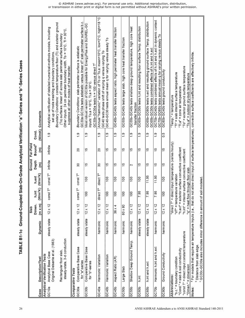
26 ANSI/ASHRAE Addendum a to ANSI/ASHRAE Standard 140-2011
TAB
LE
B1-
1cG
rou
nd
-Co
up
led
Sla
b-O
n-G
rad
eA
nal
ytic
alV
erif
icat
ion
“a”-
Ser
ies
and
“b”-
Ser
ies
Cas
es
© ASHRAE (www.ashrae.org). For personal use only. Additional reproduction, distribution, or transmission in either print or digital form is not permitted without ASHRAE's prior written permission.
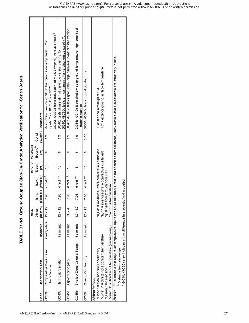
ANSI/ASHRAE Addendum a to ANSI/ASHRAE Standard 140-2011 27
TAB
LE
B1-
1dG
rou
nd
-Co
up
led
Sla
b-O
n-G
rad
eA
nal
ytic
alV
erif
icat
ion
“c”-
Ser
ies
Cas
es
© ASHRAE (www.ashrae.org). For personal use only. Additional reproduction, distribution, or transmission in either print or digital form is not permitted without ASHRAE's prior written permission.
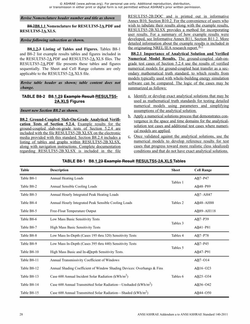
© ASHRAE (www.ashrae.org). For personal use only. Additional reproduction, distribution, or transmission in either print or digital form is not permitted without ASHRAE's prior written permission.
B8.2B8.1.1 Nomenclature for RESULTS5-2A.PDF andRESULTS5-2A.XLS.
B8.1.2.3 Listing of Tables and Figures. Tables B8-1and B8-2 list example results tables and figures included inthe RESULTS5-2A.PDF and RESULTS5-2A.XLS files. TheRESULTS5-2A.PDF file presents these tables and figuressequentially. The Sheet and Cell Range columns are onlyapplicable to the RESULTS5-2A.XLS file.
TABLE B8-2 B8.1.23 Example Result RESULTS5-2A.XLS Figures
B8.2 Ground-Coupled Slab-On-Grade Analytical Verifi-cation Tests of Section 5.2.4. Example results for theground-coupled slab-on-grade tests of Section 5.2.4 areincluded with the file RESULTS5-2B.XLSX on the electronicmedia provided with this standard. Section B8.2.4 includes alisting of tables and graphs within RESULTS5-2B.XLSX,along with navigation instructions. Complete documentationregarding RESULTS5-2B.XLSX is included in the file
RESULTS5-2B.DOC and is printed out in informativeAnnex B10, Section B10.2. For the convenience of users whowish to tabulate their results along with the example results,RESULTS5-2B.XLSX provides a method for incorporatinguser results. For a summary of how example results weredeveloped, see Informative Annex B11, Section B11.2. Moredetailed information about the example results is included inthe originating NREL/IEA research report.A-7
B8.2.1 Importance of Analytical Solution and VerifiedNumerical Model Results. The ground-coupled slab-on-grade test cases of Section 5.2.4 use the results of verifiednumerical models for ground-coupled heat transfer as a sec-ondary mathematical truth standard, to which results frommodels typically used with whole-building energy simulationsoftware can be compared. The logic of the cases may besummarized as follows:
a. Identify or develop exact analytical solutions that may beused as mathematical truth standards for testing detailednumerical models using parameters and simplifyingassumptions of the analytical solution.
b. Apply a numerical solutions process that demonstrates con-vergence in the space and time domains for the analytical-solution test cases and additional test cases where numeri-cal models are applied.
c. Once validated against the analytical solutions, use thenumerical models to develop reference results for testcases that progress toward more realistic (less idealized)conditions and that do not have exact analytical solutions.
Revise Nomenclature header number and title as shown
Revise following subsection as shown.
Revise table header as shown; table content does notchange.
Insert new Section B8.2 as shown.
TABLE B8-1 B8.1.23 Example Result RESULTS5-2A.XLS Tables
Table Description Sheet Cell Range
Table B8-1 Annual Heating LoadsTables 1
AB7–P47
Table B8-2 Annual Sensible Cooling Loads AB48–P89
Table B8-3 Annual Hourly Integrated Peak Heating Loads
Tables 2
AB7–AH47
Table B8-4 Annual Hourly Integrated Peak Sensible Cooling Loads AB48–AH88
Table B8-5 Free-Float Temperature Output AB89–AH118
Table B8-6 Low Mass Basic Sensitivity TestsTables 3
AB7–P39
Table B8-7 High Mass Basic Sensitivity Tests AB41–P81
Table B8-8 Low Mass In-Depth (Cases 195 thru 320) Sensitivity Tests Tables 4 AB7–P78
Table B8-9 Low Mass In-Depth (Cases 395 thru 440) Sensitivity TestsTables 5
AB7–P45
Table B8-10 High Mass Basic and In-dDepth Sensitivity Tests. AB47–P91
Table B8-11 Annual Transmissivity Coefficient of Windows
Tables 6
AB7–O14
Table B8-12 Annual Shading Coefficient of Window Shading Devices: Overhangs & Fins AB16–O23
Table B8-13 Case 600 Annual Incident Solar Radiation (kWh/m2) AB25–O34
Table B8-14 Case 600 Annual Transmitted Solar Radiation—Unshaded (kWh/m2) AB36–O42
Table B8-15 Case 600 Annual Transmitted Solar Radiation—Shaded (kWh/m2) AB44–O50
28 ANSI/ASHRAE Addendum a to ANSI/ASHRAE Standard 140-2011
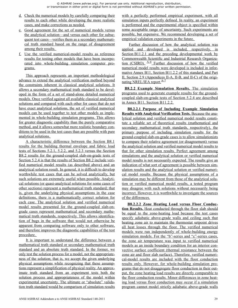
© ASHRAE (www.ashrae.org). For personal use only. Additional reproduction, distribution, or transmission in either print or digital form is not permitted without ASHRAE's prior written permission.
d. Check the numerical models by carefully comparing theirresults to each other while developing the more realisticcases, and make corrections as needed.
e. Good agreement for the set of numerical models versusthe analytical solution—and versus each other for subse-quent test cases—verifies them as a secondary mathemati-cal truth standard based on the range of disagreementamong their results.
f. Use the verified numerical-model results as referenceresults for testing other models that have been incorpo-rated into whole-building simulation computer pro-grams.
This approach represents an important methodologicaladvance to extend the analytical verification method beyondthe constraints inherent in classical analytical solutions. Itallows a secondary mathematical truth standard to be devel-oped in the form of a set of stand-alone detailed numericalmodels. Once verified against all available classical analyticalsolutions and compared with each other for cases that do nothave exact analytical solutions, the set of verified numericalmodels can be used together to test other models as imple-mented in whole-building simulation programs. This allowsfor greater diagnostic capability than the purely comparativemethod, and it allows somewhat more realistic boundary con-ditions to be used in the test cases than are possible with pureanalytical solutions.
A characteristic difference between the Section B8.1results for the building thermal envelope and fabric loadtests of Sections 5.2.1, 5.2.2, and 5.2.3 versus the SectionB8.2 results for the ground-coupled slab-on-grade tests ofSection 5.2.4 is that the results of Section B8.2 include veri-fied numerical model results (as described above) and ananalytical solution result. In general, it is difficult to developworthwhile test cases that can be solved analytically, butsuch solutions are extremely useful when possible. Analyti-cal solutions (or quasi-analytical solutions for some cases ofother sections) represent a mathematical truth standard; thatis, given the underlying physical assumptions in the casedefinitions, there is a mathematically correct solution foreach case. The analytical solution and verified numericalmodel results presented for the ground-coupled slab-on-grade cases represent mathematical and secondary mathe-matical truth standards, respectively. This allows identifica-tion of bugs in the software that would not otherwise beapparent from comparing software only to other software,and therefore improves the diagnostic capabilities of the testprocedure.
It is important to understand the difference between amathematical truth standard or secondary mathematical truthstandard and an absolute truth standard. In the former, weonly test the solution process for a model, not the appropriate-ness of the solution; that is, we accept the given underlyingphysical assumptions while recognizing that these assump-tions represent a simplification of physical reality. An approx-imate truth standard from an experiment tests both thesolution process and appropriateness of the model withinexperimental uncertainty. The ultimate or “absolute” valida-tion truth standard would be comparison of simulation results
with a perfectly performed empirical experiment, with allsimulation inputs perfectly defined. In reality, an experimentis performed and the experimental object is specified withinsome acceptable range of uncertainty. Such experiments arepossible, but expensive. We recommend developing a set ofempirical validation experiments in the future.
Further discussion of how the analytical solution wasapplied and developed is included, respectively, inSection B11.2.1 and the preceding developmental work byCommonwealth Scientific and Industrial Research Organiza-tion (CSIRO). A-4 Further discussion of how the verifiednumerical model results were developed is included in infor-mative Annex B11, Section B11.2.2 of this standard, and PartII, Section 2.9 (Appendices II-A, II-B, and II-C) of the origi-nating NREL/IEA report.A-7
B8.2.2 Example Simulation Results. The simulationprograms used to generate example results for the ground-coupled slab-on-grade tests of Section 5.2.4 are describedin Annex B11, Section B11.2.2.
B8.2.2.1 Purpose of Including Example SimulationResults with Analytical Verification Tests. Because the ana-lytical solution and verified numerical model results consti-tute a reliable set of theoretical results (mathematical andsecondary mathematical truth standards, respectively), theprimary purpose of including simulation results for theground-coupled slab-on-grade cases is to allow simulationiststo compare their relative agreement (or disagreement) versusthe analytical solution and verified numerical model results tothat for other simulation results. Perfect agreement amongsimulations and the analytical solution or verified numericalmodel results is not necessarily expected. The results give anindication of what sort of agreement is possible between sim-ulation results and the analytical solution or verified numeri-cal model results. Because the physical assumptions of asimulation may be different from those of the analytical solu-tion or verified numerical model results, a tested programmay disagree with such solutions without necessarily beingincorrect. However, it is worthwhile to investigate the sourcesof the differences.
B8.2.2.2 Zone Heating Load versus Floor Conduc-tion Results. Heat conducted through the floor slab shouldbe equal to the zone-heating load because the test casesspecify adiabatic above-grade walls and ceiling such thatheating zone air to maintain the thermostat setpoint drivesall heat losses through the floor. The verified numericalmodels were run independently of whole-building energysimulation models. For the “b”-series and “c”-series cases,the zone air temperature was input to verified numericalmodels as an inside boundary condition for an interior con-vective surface coefficient (thermal resistance between thezone air and floor slab surface). Therefore, verified numeri-cal-model results are included with the floor conductionresults only. However, for whole-building simulation pro-grams that do not disaggregate floor conduction in their out-put, the zone heating load results are directly comparable tothe floor conduction results. Minor differences in zone heat-ing load versus floor conduction may occur if a simulationprogram cannot model strictly adiabatic above-grade walls
ANSI/ASHRAE Addendum a to ANSI/ASHRAE Standard 140-2011 29
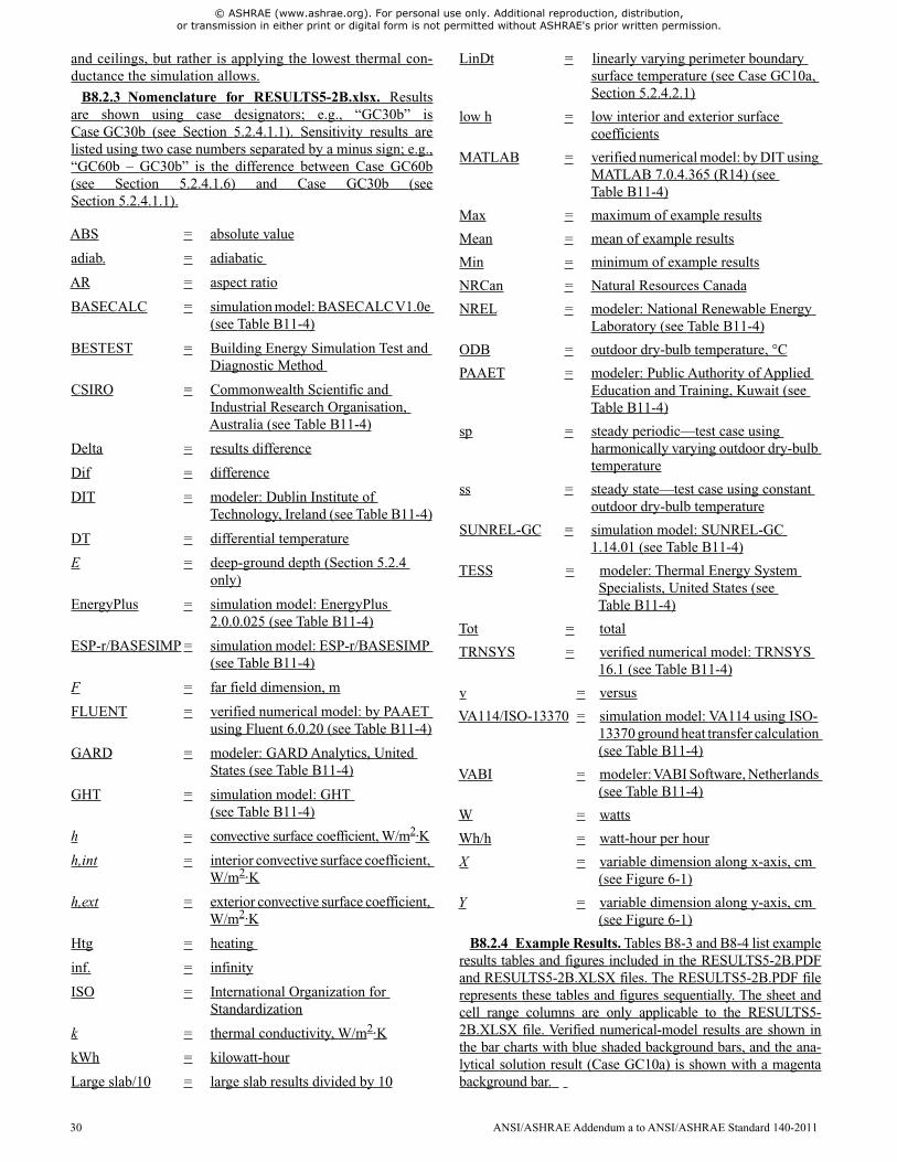
© ASHRAE (www.ashrae.org). For personal use only. Additional reproduction, distribution, or transmission in either print or digital form is not permitted without ASHRAE's prior written permission.
and ceilings, but rather is applying the lowest thermal con-ductance the simulation allows.
B8.2.3 Nomenclature for RESULTS5-2B.xlsx. Resultsare shown using case designators; e.g., “GC30b” isCase GC30b (see Section 5.2.4.1.1). Sensitivity results arelisted using two case numbers separated by a minus sign; e.g.,“GC60b – GC30b” is the difference between Case GC60b(see Section 5.2.4.1.6) and Case GC30b (seeSection 5.2.4.1.1).
ABS = absolute value
adiab. = adiabatic
AR = aspect ratio
BASECALC = simulation model: BASECALCV1.0e(see Table B11-4)
BESTEST = Building Energy Simulation Test andDiagnostic Method
CSIRO = Commonwealth Scientific andIndustrial Research Organisation,Australia (see Table B11-4)
Delta = results difference
Dif = difference
DIT = modeler: Dublin Institute ofTechnology, Ireland (see Table B11-4)
DT = differential temperature
E = deep-ground depth (Section 5.2.4only)
EnergyPlus = simulation model: EnergyPlus2.0.0.025 (see Table B11-4)
ESP-r/BASESIMP = simulation model: ESP-r/BASESIMP(see Table B11-4)
F = far field dimension, m
FLUENT = verified numerical model: by PAAETusing Fluent 6.0.20 (see Table B11-4)
GARD = modeler: GARD Analytics, UnitedStates (see Table B11-4)
GHT = simulation model: GHT(see Table B11-4)
h = convective surface coefficient, W/m2·K
h,int = interior convective surface coefficient,W/m2·K
h,ext = exterior convective surface coefficient,W/m2·K
Htg = heating
inf. = infinity
ISO = International Organization forStandardization
k = thermal conductivity, W/m2·K
kWh = kilowatt-hour
Large slab/10 = large slab results divided by 10
LinDt = linearly varying perimeter boundarysurface temperature (see Case GC10a,Section 5.2.4.2.1)
low h = low interior and exterior surfacecoefficients
MATLAB = verified numerical model: by DIT usingMATLAB 7.0.4.365 (R14) (seeTable B11-4)
Max = maximum of example results
Mean = mean of example results
Min = minimum of example results
NRCan = Natural Resources Canada
NREL = modeler: National Renewable EnergyLaboratory (see Table B11-4)
ODB = outdoor dry-bulb temperature, °C
PAAET = modeler: Public Authority of AppliedEducation and Training, Kuwait (seeTable B11-4)
sp = steady periodic—test case usingharmonically varying outdoor dry-bulbtemperature
ss = steady state—test case using constantoutdoor dry-bulb temperature
SUNREL-GC = simulation model: SUNREL-GC1.14.01 (see Table B11-4)
TESS = modeler: Thermal Energy SystemSpecialists, United States (seeTable B11-4)
Tot = total
TRNSYS = verified numerical model: TRNSYS16.1 (see Table B11-4)
v = versus
VA114/ISO-13370 = simulation model: VA114 using ISO-13370 ground heat transfer calculation(see Table B11-4)
VABI = modeler:VABI Software, Netherlands(see Table B11-4)
W = watts
Wh/h = watt-hour per hour
X = variable dimension along x-axis, cm(see Figure 6-1)
Y = variable dimension along y-axis, cm(see Figure 6-1)
B8.2.4 Example Results. Tables B8-3 and B8-4 list exampleresults tables and figures included in the RESULTS5-2B.PDFand RESULTS5-2B.XLSX files. The RESULTS5-2B.PDF filerepresents these tables and figures sequentially. The sheet andcell range columns are only applicable to the RESULTS5-2B.XLSX file. Verified numerical-model results are shown inthe bar charts with blue shaded background bars, and the ana-lytical solution result (Case GC10a) is shown with a magentabackground bar.
30 ANSI/ASHRAE Addendum a to ANSI/ASHRAE Standard 140-2011
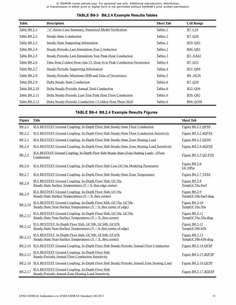
© ASHRAE (www.ashrae.org). For personal use only. Additional reproduction, distribution, or transmission in either print or digital form is not permitted without ASHRAE's prior written permission.
TABLE B8-3 B8.2.4 Example Results Tables
Table Description Sheet Tab Cell Range
Table B8.2-1 “a”-Series Case Summary, Numerical Model Verification Tables 1 B7–L24
Table B8.2-2 Steady-State Conduction Tables 2 B7–Q26
Table B8.2-3 Steady-State Supporting Information Tables 2 B29–Q42
Table B8.2-4 Steady-Periodic Last-Simulation-Year Conduction Tables 2 B46–Q83
Table B8.2-5 Steady-Periodic Last-Simulation-Year Peak-Hour Conduction Tables 3 B7–AA62
Table B8.2-6 Time from Coldest Hour (Jan 15, Hour 4) to Peak Conduction Occurrence Tables 4 B7–Q33
Table B8.2-7 Steady-Periodic Supporting Information Tables 4 B35–Q60
Table B8.2-8 Steady-Periodic Minimum ODB and Time of Occurrence Tables 5 B8–AE38
Table B8.2-9 Delta Steady-State Conduction Tables 6 B7–Q30
Table B8.2-10 Delta Steady-Periodic Annual Total Conduction Tables 6 B32–Q56
Table B8.2-11 Delta Steady-Periodic Last-Year Peak Hour Floor Conduction Tables 6 B58–Q82
Table B8.2-12 Delta Steady-Periodic Conduction v Coldest Hour Phase Shift Tables 6 B84–Q108
TABLE B8-4 B8.2.4 Example Results Figures
Figure Title Sheet Tab
B8.2-1 IEA BESTEST Ground Coupling: In-Depth Floor Slab Steady-State Floor Conduction Figure B8.2-1 QFSS
B8.2-2 IEA BESTEST Ground Coupling: In-Depth Floor Slab Steady-State Floor Conduction Sensitivity Figure B8.2-2 dQFSS
B8.2-3 IEA BESTEST Ground Coupling: In-Depth Floor Slab Steady-State Zone Heating Load Figure B8.2-3 QZSS
B8.2-4 IEA BESTEST Ground Coupling: In-Depth Floor Slab Steady-State Zone Heating Load Sensitivity Figure B8.2-4 dQZSS
B8.2-5IEA BESTEST Ground Coupling: In-Depth Floor Slab Steady-State (Zone Heating Load)—(FloorConduction)
Figure B8.2-5 QZ-FSS
B8.2-6 IEA BESTEST Ground Coupling: In-Depth Floor Slab Case GC10a Modeling ParametersFigure B8.2-6GC10Par
B8.2-7 IEA BESTEST Ground Coupling: In-Depth Floor Slab Steady-State Zone Temperature Figure B8.2-7 TZSS
B8.2-8IEA BESTEST Ground Coupling: In-Depth Floor Slab, GC10aSteady-State Surface Temperatures (Y = 0, thru edge center)
Figure B8.2-8TempGC10a-Surf
B8.2-9IEA BESTEST Ground Coupling: In-Depth Floor Slab, GC10aSteady-State Surface Temperatures (Y = X, thru corner)
Figure B8.2-9TempGC10a-Surf-diag
B8.2-10IEA BESTEST Ground Coupling: In-Depth Floor Slab, GC10a, GC30aSteady-State Near-Surface Temperatures (Y = 0, thru center of edge)
Figure B8.2-10TempGC10a-30a
B8.2-11IEA BESTEST Ground Coupling: In-Depth Floor Slab, GC10a, GC30aSteady-State Near-Surface Temperatures (Y = X, thru corner)
Figure B8.2-11TempGC10a-30a-diag
B8.2-12IEA BESTEST: In-Depth Floor Slab, GC30b, GC60b, GC65bSteady-State Near-Surface Temperatures (Y = 0, thru center of edge)
Figure B8.2-12TempGC30b-65b
B8.2-13IEA BESTEST: In-Depth Floor Slab, GC30b, GC60b, GC65bSteady-State Near-Surface Temperatures (Y = X, thru corner)
Figure B8.2-13TempGC30b-65b-diag
B8.2-14 IEA BESTEST Ground Coupling: In-Depth Floor Slab Steady-Periodic Annual Floor Conduction Figure B8.2-14 QFSP
B8.2-15IEA BESTEST Ground Coupling: In-Depth Floor SlabSteady-Periodic Annual Floor Conduction Sensitivity
Figure B8.2-15 dQFSP
B8.2-16 IEA BESTEST Ground Coupling: In-Depth Floor Slab Steady-Periodic Annual Zone Heating Load Figure B8.2-16 QZSP
B8.2-17IEA BESTEST Ground Coupling: In-Depth Floor SlabSteady-Periodic Annual Zone Heating Load Sensitivity
Figure B8.2-17 dQZSP
ANSI/ASHRAE Addendum a to ANSI/ASHRAE Standard 140-2011 31
© ASHRAE (www.ashrae.org). For personal use only. Additional reproduction, distribution, or transmission in either print or digital form is not permitted without ASHRAE's prior written permission.
INFORMATIVE ANNEX B9DIAGNOSING THE RESULTS USING THEFLOW DIAGRAMS
B9.1 General Description. Figures B9-1 through B9-107contain a set of flow diagrams that serve as a guide for diag-nosing the cause of disagreeing results that may arise fromusing this method of test. These flow diagrams list the fea-ture(s) being tested, thus indicating potential sources of algo-rithmic differences.
B9.2 Comparing Tested Software Results to Other Exam-ple Results
B9.2.1 “Example results” are either results presented ininformative Annexes B8 and B16 or other results that weregenerated using this standard method of test.
B9.2.2 In this annex we provide no formal criteria for whenresults agree or disagree. Determination of when results agreeor disagree is left to the user. In making this determination,the user should consider
a. magnitude of results for individual cases,
b. magnitude of difference in results between certain cases(e.g., “Case 610-Case 600”),
c. same direction of sensitivity (positive or negative) for dif-ference in results between certain cases (e.g., Case 610–Case 600),
d. if results are logically counterintuitive with respect toknown or expected physical behavior,
e. availability of analytical or quasi-analytical solutionresults (i.e., mathematical truth standard as described ininformative Annex B16, Section B16.2), or verifiednumerical-model results (see Annex B8, Section B8.2.1),
f. for analytical verification test cases, the degree of dis-agreement that occurred for other simulation results inAnnex B16 versus the quasi-analytical or analytical solu-
B8.2-18IEA BESTEST Ground Coupling: In-Depth Floor SlabSteady-Periodic (Zone Heating Load) – (Floor Conduction)
Figure B8.2-18 QZ-FSP
B8.2-19IEA BESTEST Ground Coupling: In-Depth Floor SlabHourly Floor Conduction, GC40a
Figure B8.2-19GC40aHourly-1
B8.2-20IEA BESTEST Ground Coupling: In-Depth Floor SlabHourly Floor Conduction, GC40b
Figure B8.2-20GC40bHourly-2
B8.2-21IEA BESTEST Ground Coupling: In-Depth Floor SlabHourly Floor Conduction, GC40c
Figure B8.2-21GC40cHourly-1
B8.2-22IEA BESTEST Ground Coupling: In-Depth Floor SlabSteady-Periodic Phase Shift, Time from Coldest ODB to Peak Floor Conduction
Figure B8.2-22 PhF
B8.2-23IEA BESTEST Ground Coupling: In-Depth Floor SlabSteady-Periodic Phase Shift Sensitivity, Floor Conduction v. ODB
Figure B8.2-23 dPhF
B8.2-24IEA BESTEST Ground Coupling: In-Depth Floor SlabSteady-Periodic Phase Shift, Time from Coldest ODB to Peak Zone Load
Figure B8.2-24 PhZ
B8.2-25IEA BESTEST Ground Coupling: In-Depth Floor SlabDelta Steady-Periodic Phase Shift Sensitivity, Zone Load v. ODB
Figure B8.2-25 dPhZ
B8.2-26IEA BESTEST Ground Coupling: In-Depth Floor SlabSteady-Periodic Annual Peak-Hour Floor Conduction
Figure B8.2-26 PFSP
B8.2-27IEA BESTEST Ground Coupling: In-Depth Floor SlabSteady-Periodic Annual Peak-Hour Floor Conduction Sensitivity
Figure B8.2-27 dPFSP
B8.2-28IEA BESTEST Ground Coupling: In-Depth Floor SlabSteady-Periodic Annual Peak-Hour Zone Heating Load
Figure B8.2-28 PZSP
B8.2-29IEA BESTEST Ground Coupling: In-Depth Floor SlabSteady-Periodic Annual Peak-Hour Zone Heating Load Sensitivity
Figure B8.2-29 dPZSP
B8.2-30IEA BESTEST Ground Coupling: In-Depth Floor SlabSteady-Periodic (Peak Zone Heating Load) – (Peak Floor Conduction)
Figure B8.2-30 PZ-FSP
B8.2-31IEA BESTEST Ground Coupling: In-Depth Floor SlabSteady-Periodic Zone Temperature
Figure B8.2-31 TZSP
B8.2-32IEA BESTEST Ground Coupling: In-Depth Floor SlabSteady-Periodic Minimum ODB
Figure B8.2-32ODBmin
TABLE B8-4 B8.2.4 Example Results Figures (Continued)
Figure Title Sheet Tab
Revise Annex B9 as shown. New Figures B9-5, B9-6, andB9-7 are included at the end of the text of this annex; cur-rent figures B9-5, B9-6, and B9-7 are renumbered to B9-8,B9-9, and B9-10 respectively.
32 ANSI/ASHRAE Addendum a to ANSI/ASHRAE Standard 140-2011
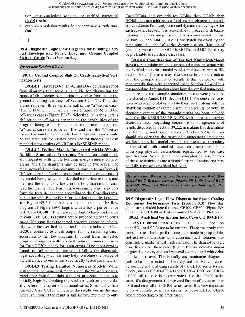
© ASHRAE (www.ashrae.org). For personal use only. Additional reproduction, distribution, or transmission in either print or digital form is not permitted without ASHRAE's prior written permission.
tion, quasi-analytical solution, or verified numericalmodel results,
g. example simulation results do not represent a truth stan-dard.
[ . . . ]
B9.4 Diagnostic Logic Flow Diagrams for Building Ther-mal Envelope and Fabric Load and Ground-CoupledSlab-on-Grade Tests (Section 5.2)
B9.4.4 Ground-Coupled Slab-On-Grade Analytical Veri-fication Tests
B9.4.4.1 Figures B9-5, B9-6, and B9-7 contain a set offlow diagrams that serve as a guide for diagnosing thecause of disagreeing results that may arise from using theground coupling test cases of Section 5.2.4. The flow dia-grams represent three separate paths: the “a”-series cases(Figure B9-5), the “b”-series cases (Figure B9-6), and the“c”-series cases (Figure B9-7). Selecting “a”-series versus“b”-series or “c”-series depends on the capabilities of theprogram being tested. For detailed numerical models, the“a”-series cases are to be run first and then the “b” seriescases. For most other models, the “b”-series cases shouldbe run first. The “c”-series cases are for models that canmatch the constraints of NRCan’s BASESIMP model.
B9.4.4.2 Testing Models Integrated within Whole-Building Simulation Programs. For slab-on-grade mod-els integrated with whole-building energy simulation pro-grams, the flow diagrams may be used in two ways. Themost powerful but time-consuming way is to perform all“b”-series and “c”-series cases (and the “a”-series cases ifthe model being tested is a detailed numerical model), andthen use the diagnostic logic in the flow diagrams to ana-lyze the results. The least time-consuming way is to per-form the tests in sequence according to the flow diagrams,beginning with Figure B9-5 for detailed numerical modelsand Figure B9-6 for other less detailed models. The flowdiagram of Figure B9-6 begins with a basic performancetest (Case GC30b). It is very important to have confidencein your Case GC30b results before proceeding to the othercases. If output from the tested program agrees satisfacto-rily with the verified numerical-model results for CaseGC30b, continue to check output for the remaining casesaccording to the flow diagram. If output from the testedprogram disagrees with verified numerical-model resultsfor Case GC30b, check for input errors. If no input error isfound, run all other test cases and follow the diagnosticlogic accordingly, as this may help to isolate the source ofthe difference to one of the specifically tested parameters.
B9.4.4.3 Testing Detailed Numerical Models. Whentesting detailed numerical models with the “a”-series cases,experience from field trials of the test procedure indicates toinitially begin by checking the results of each case individu-ally before moving on to additional cases. Specifically, firstrun only Case GC10a and check the results versus the ana-lytical solution. If the result is satisfactory, move on to only
Case GC30a, and similarly for GC40a, then GC30b, thenGC40b, as each addresses a fundamental change in bound-ary conditions for steady-state and dynamic modeling. Aftereach case is checked, it is reasonable to proceed with batch-running the remaining cases: it is recommended to runGC60b, GC65b, and GC30c as one batch followed by theremaining “b”- and “c”-series dynamic cases. Because ofgeometry variations for GC45b, GC45c, and GC50c, it maybe preferable to run those cases last.
B9.4.4.4 Consideration of Verified Numerical-ModelResults. At a minimum, the user should compare output withthe verified numerical-model results provided in Annex B8,Section B8.2. The user may also choose to compare outputwith the example simulation results in that section, or withother results that were generated using Section 5.2.4 of thistest procedure. Information about how the verified numerical-model results and example simulation results were producedis included in Annex B11, Section B11.2. For convenience tousers who wish to plot or tabulate their results along with theanalytical solution or example simulation results, or both, anelectronic version of the example results has been includedwith the file RESULTS5-2B.XLSX with the accompanyingelectronic files. Regarding determination of agreement ofresults discussed in Section B9.2.2, in making this determina-tion for the ground coupling tests of Section 5.2.4, the usershould consider that the range of disagreement among theverified numerical-model results represents a secondarymathematical truth standard based on acceptance of theunderlying physical assumptions represented by the casespecifications. Note that the underlying physical assumptionsof the case definitions are a simplification of reality and maynot fully represent empirical behavior.
B9.5 Diagnostic Logic Flow Diagram for Space CoolingEquipment Performance Tests (Section 5.3). Flow dia-grams are included here for cases CE100–CE200 (Figure B9-85) and cases CE300–CE545 (Figures B9-96 and B9-107).
B9.5.1 Analytical Verification Tests, Cases CE100-CE200B9.5.1.1 Introduction. Cases CE100–CE200 (see Sec-
tions 5.3.1 and 5.3.2) are to be run first. These are steady-statecases that test basic performance map modeling capabilitiesand utilize comparisons with quasi-analytical solutions thatconstitute a mathematical truth standard. The diagnostic logicflow diagram for these cases (Figure B9-85) indicates similardiagnostics for dry-coil and wet-coil (without and with dehu-midification) cases. This is really one continuous diagnosticpath to be implemented for both dry-coil and wet-coil cases.Performing and analyzing results of the CE100 series tests inblocks, such as CE100–CE140 and CE150–CE200, or CE100–CE200, all at once is recommended. For the CE100 seriescases, if a disagreement is uncovered for one of the cases, thenfix it and rerun all the CE100 series cases. It is very importantto have confidence in the results for cases CE100–CE200before proceeding to the other cases.
Insert new Section B9.4.4.
Revise section B9.5 as shown. Insert new figures B9-5, B9-6, and B9-7. Rename current figures B9-5, B9-6, and B9-7to B9-8, B9-9, and B9-10 respectively, as shown after thenew figures.
ANSI/ASHRAE Addendum a to ANSI/ASHRAE Standard 140-2011 33
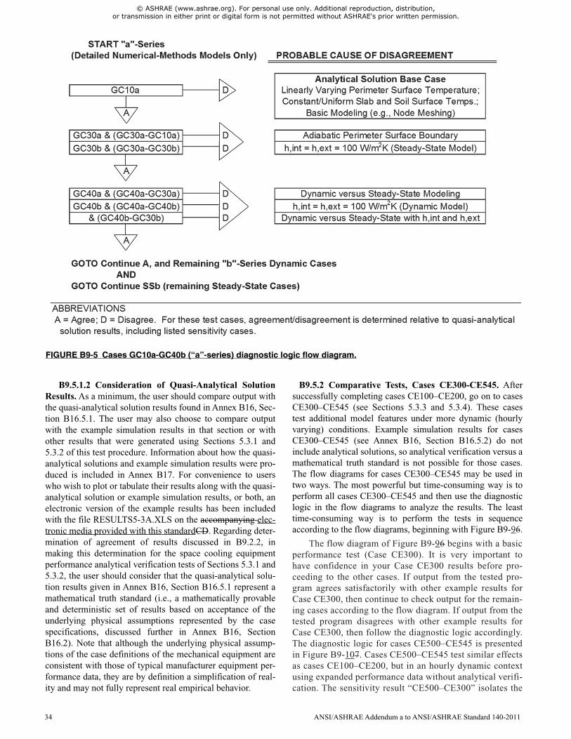
© ASHRAE (www.ashrae.org). For personal use only. Additional reproduction, distribution, or transmission in either print or digital form is not permitted without ASHRAE's prior written permission.
B9.5.1.2 Consideration of Quasi-Analytical SolutionResults. As a minimum, the user should compare output withthe quasi-analytical solution results found in Annex B16, Sec-tion B16.5.1. The user may also choose to compare outputwith the example simulation results in that section or withother results that were generated using Sections 5.3.1 and5.3.2 of this test procedure. Information about how the quasi-analytical solutions and example simulation results were pro-duced is included in Annex B17. For convenience to userswho wish to plot or tabulate their results along with the quasi-analytical solution or example simulation results, or both, anelectronic version of the example results has been includedwith the file RESULTS5-3A.XLS on the accompanying elec-tronic media provided with this standardCD. Regarding deter-mination of agreement of results discussed in B9.2.2, inmaking this determination for the space cooling equipmentperformance analytical verification tests of Sections 5.3.1 and5.3.2, the user should consider that the quasi-analytical solu-tion results given in Annex B16, Section B16.5.1 represent amathematical truth standard (i.e., a mathematically provableand deterministic set of results based on acceptance of theunderlying physical assumptions represented by the casespecifications, discussed further in Annex B16, SectionB16.2). Note that although the underlying physical assump-tions of the case definitions of the mechanical equipment areconsistent with those of typical manufacturer equipment per-formance data, they are by definition a simplification of real-ity and may not fully represent real empirical behavior.
B9.5.2 Comparative Tests, Cases CE300-CE545. Aftersuccessfully completing cases CE100–CE200, go on to casesCE300–CE545 (see Sections 5.3.3 and 5.3.4). These casestest additional model features under more dynamic (hourlyvarying) conditions. Example simulation results for casesCE300–CE545 (see Annex B16, Section B16.5.2) do notinclude analytical solutions, so analytical verification versus amathematical truth standard is not possible for those cases.The flow diagrams for cases CE300–CE545 may be used intwo ways. The most powerful but time-consuming way is toperform all cases CE300–CE545 and then use the diagnosticlogic in the flow diagrams to analyze the results. The leasttime-consuming way is to perform the tests in sequenceaccording to the flow diagrams, beginning with Figure B9-96.
The flow diagram of Figure B9-96 begins with a basicperformance test (Case CE300). It is very important tohave confidence in your Case CE300 results before pro-ceeding to the other cases. If output from the tested pro-gram agrees satisfactorily with other example results forCase CE300, then continue to check output for the remain-ing cases according to the flow diagram. If output from thetested program disagrees with other example results forCase CE300, then follow the diagnostic logic accordingly.The diagnostic logic for cases CE500–CE545 is presentedin Figure B9-107. Cases CE500–CE545 test similar effectsas cases CE100–CE200, but in an hourly dynamic contextusing expanded performance data without analytical verifi-cation. The sensitivity result “CE500–CE300” isolates the
FIGURE B9-5 Cases GC10a-GC40b (“a”-series) diagnostic logic flow diagram.
34 ANSI/ASHRAE Addendum a to ANSI/ASHRAE Standard 140-2011
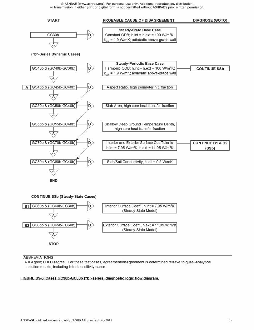
© ASHRAE (www.ashrae.org). For personal use only. Additional reproduction, distribution, or transmission in either print or digital form is not permitted without ASHRAE's prior written permission.
FIGURE B9-6 Cases GC30b-GC80b (“b”-series) diagnostic logic flow diagram.
ANSI/ASHRAE Addendum a to ANSI/ASHRAE Standard 140-2011 35
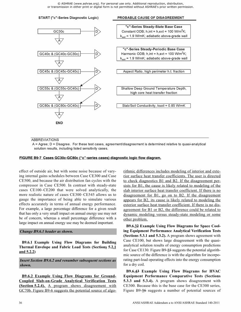
© ASHRAE (www.ashrae.org). For personal use only. Additional reproduction, distribution, or transmission in either print or digital form is not permitted without ASHRAE's prior written permission.
effect of outside air, but with some noise because of vary-ing internal gains schedules between Case CE300 and CaseCE500, and because the air distribution fan cycles with thecompressor in Case CE500. In contrast with steady-statecases CE100–CE200 that were solved analytically, themore realistic nature of cases CE300–CE545 allows us togauge the importance of being able to simulate variouseffects accurately in terms of annual energy performance.For example, a large percentage difference for a given resultthat has only a very small impact on annual energy use may notbe of concern, whereas a small percentage difference with alarge impact on annual energy use may be deemed important.
B9.6.1 Example Using Flow Diagrams for BuildingThermal Envelope and Fabric Load Tests (Sections 5.2.1and 5.2.2)
B9.6.2 Example Using Flow Diagrams for Ground-Coupled Slab-on-Grade Analytical Verification Tests(Section 5.2.4). A program shows disagreement withGC70b. Figure B9-6 suggests the potential source of algo-
rithmic differences includes modeling of interior and exte-rior surface heat transfer coefficients. The user is directedto check diagnostics B1 and B2. If the disagreement per-sists for B1, the cause is likely related to modeling of theslab interior surface heat transfer coefficient. If there is nodisagreement for B1, go on to B2. If the disagreementappears for B2, its cause is likely related to modeling theexterior surface heat transfer coefficient. If there is no dis-agreement for B1 or B2, the difference could be related todynamic modeling versus steady-state modeling or someother problem.
B9.6.32 Example Using Flow Diagrams for Space Cool-ing Equipment Performance Analytical Verification Tests(Sections 5.3.1 and 5.3.2). A program shows agreement withCase CE100, but shows large disagreement with the quasi-analytical solution results of energy consumption predictionsfor Case CE130. Figure B9-85 suggests the potential algorith-mic source of the difference is with the algorithm for incorpo-rating part-load operating effects into the energy consumptionfor a dry coil.
B9.6.43 Example Using Flow Diagrams for HVACEquipment Performance Comparative Tests (Sections5.3.3 and 5.3.4). A program shows disagreement withCE300. Because this is the base case for the CE300 series,Figure B9-96 suggests a number of potential sources of
Change B9.6.1 header as shown.
Insert Section B9.6.2 and renumber subsequent sections asshown.
FIGURE B9-7 Cases GC30c-GC80c (“c”-series cases) diagnostic logic flow diagram.
36 ANSI/ASHRAE Addendum a to ANSI/ASHRAE Standard 140-2011
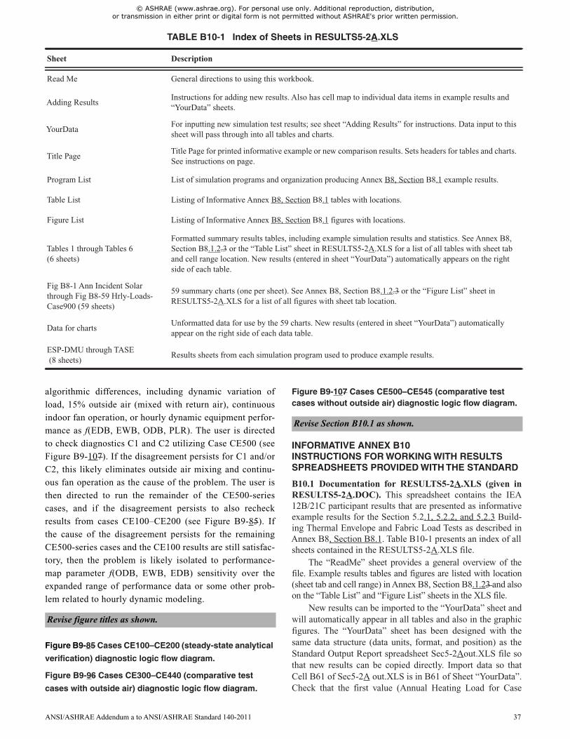
© ASHRAE (www.ashrae.org). For personal use only. Additional reproduction, distribution, or transmission in either print or digital form is not permitted without ASHRAE's prior written permission.
algorithmic differences, including dynamic variation ofload, 15% outside air (mixed with return air), continuousindoor fan operation, or hourly dynamic equipment perfor-mance as f(EDB, EWB, ODB, PLR). The user is directedto check diagnostics C1 and C2 utilizing Case CE500 (seeFigure B9-107). If the disagreement persists for C1 and/orC2, this likely eliminates outside air mixing and continu-ous fan operation as the cause of the problem. The user isthen directed to run the remainder of the CE500-seriescases, and if the disagreement persists to also recheckresults from cases CE100–CE200 (see Figure B9-85). Ifthe cause of the disagreement persists for the remainingCE500-series cases and the CE100 results are still satisfac-tory, then the problem is likely isolated to performance-map parameter f(ODB, EWB, EDB) sensitivity over theexpanded range of performance data or some other prob-lem related to hourly dynamic modeling.
Figure B9-85 Cases CE100–CE200 (steady-state analytical
verification) diagnostic logic flow diagram.
Figure B9-96 Cases CE300–CE440 (comparative test
cases with outside air) diagnostic logic flow diagram.
Figure B9-107 Cases CE500–CE545 (comparative testcases without outside air) diagnostic logic flow diagram.
INFORMATIVE ANNEX B10INSTRUCTIONS FOR WORKING WITH RESULTSSPREADSHEETS PROVIDED WITH THE STANDARD
B10.1 Documentation for RESULTS5-2A.XLS (given inRESULTS5-2A.DOC). This spreadsheet contains the IEA12B/21C participant results that are presented as informativeexample results for the Section 5.2.1, 5.2.2, and 5.2.3 Build-ing Thermal Envelope and Fabric Load Tests as described inAnnex B8, Section B8.1. Table B10-1 presents an index of allsheets contained in the RESULTS5-2A.XLS file.
The “ReadMe” sheet provides a general overview of thefile. Example results tables and figures are listed with location(sheet tab and cell range) in Annex B8, Section B8.1.23 and alsoon the “Table List” and “Figure List” sheets in the XLS file.
New results can be imported to the “YourData” sheet andwill automatically appear in all tables and also in the graphicfigures. The “YourData” sheet has been designed with thesame data structure (data units, format, and position) as theStandard Output Report spreadsheet Sec5-2Aout.XLS file sothat new results can be copied directly. Import data so thatCell B61 of Sec5-2A out.XLS is in B61 of Sheet “YourData”.Check that the first value (Annual Heating Load for Case
TABLE B10-1 Index of Sheets in RESULTS5-2A.XLS
Sheet Description
Read Me General directions to using this workbook.
Adding ResultsInstructions for adding new results. Also has cell map to individual data items in example results and“YourData” sheets.
YourDataFor inputting new simulation test results; see sheet “Adding Results” for instructions. Data input to thissheet will pass through into all tables and charts.
Title PageTitle Page for printed informative example or new comparison results. Sets headers for tables and charts.See instructions on page.
Program List List of simulation programs and organization producing Annex B8, Section B8.1 example results.
Table List Listing of Informative Annex B8, Section B8.1 tables with locations.
Figure List Listing of Informative Annex B8, Section B8.1 figures with locations.
Tables 1 through Tables 6(6 sheets)
Formatted summary results tables, including example simulation results and statistics. See Annex B8,Section B8.1.2.3 or the “Table List” sheet in RESULTS5-2A.XLS for a list of all tables with sheet taband cell range location. New results (entered in sheet “YourData”) automatically appears on the rightside of each table.
Fig B8-1 Ann Incident Solarthrough Fig B8-59 Hrly-Loads-Case900 (59 sheets)
59 summary charts (one per sheet). See Annex B8, Section B8.1.2.3 or the “Figure List” sheet inRESULTS5-2A.XLS for a list of all figures with sheet tab location.
Data for chartsUnformatted data for use by the 59 charts. New results (entered in sheet “YourData”) automaticallyappear on the right side of each data table.
ESP-DMU through TASE(8 sheets)
Results sheets from each simulation program used to produce example results.
Revise figure titles as shown.
Revise Section B10.1 as shown.
ANSI/ASHRAE Addendum a to ANSI/ASHRAE Standard 140-2011 37
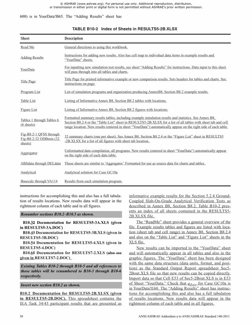
© ASHRAE (www.ashrae.org). For personal use only. Additional reproduction, distribution, or transmission in either print or digital form is not permitted without ASHRAE's prior written permission.
600) is in YourData!B65. The “Adding Results” sheet has
instructions for accomplishing this and also has a full tabula-tion of results locations. New results data will appear in therightmost column of each table and in all figures.
B10.32 Documentation for RESULTS5-3A.XLS (givenin RESULTS5-3A.DOC)
B10.43 Documentation for RESULTS5-3B.XLS (given inRESULTS5-3B.DOC)
B10.54 Documentation for RESULTS5-4.XLS (given inRESULTS5-4.DOC)
B10.65 Documentation for RESULTS7-2.XLS (also seegiven in RESULTS7-2.DOC)
B10.2 Documentation for RESULTS5-2B.XLSX (givenin RESULTS5-2B.DOC). This spreadsheet contains theIEA Task 34/43 participant results that are presented as
informative example results for the Section 5.2.4 Ground-Coupled Slab-On-Grade Analytical Verification Tests asdescribed in Annex B8, Section B8.2. Table B10-2 pres-ents an index of all sheets contained in the RESULTS5-2B.XLSX file.
The “ReadMe” sheet provides a general overview of thefile. Example results tables and figures are listed with loca-tion (sheet tab and cell range) in Annex B8, Section B8.2.4and also on the “Table List” and “Figure List” sheets in theXLS file.
New results can be imported to the “YourData” sheetand will automatically appear in all tables and also in thegraphic figures. The “YourData” sheet has been designedwith the same data structure (data units, format, and posi-tion) as the Standard Output Report spreadsheet Sec5-2Bout.XLS file so that new results can be copied directly.Import data so that Cell E53 of Sec5-2Bout.XLS is in E53of Sheet “YourData.” Check that qfloor for Case GC10a isin YourData!E60. The “Adding Results” sheet has instruc-tions for accomplishing this and also has a full tabulationof results locations. New results data will appear in therightmost column of each table and in all figures.
TABLE B10-2 Index of Sheets in RESULTS5-2B.XLSX
Sheet Description
Read Me General directions to using this workbook.
Adding ResultsInstructions for adding new results. Also has cell map to individual data items in example results and“YourData” sheets.
YourDataFor inputting new simulation test results, see sheet “Adding Results” for instructions. Data input to this sheetwill pass through into all tables and charts.
Title PageTitle Page for printed informative example or new comparison results. Sets headers for tables and charts. Seeinstructions on page.
Program List List of simulation programs and organization producing AnnexB8, Section B8.2 example results.
Table List Listing of Informative Annex B8, Section B8.2 tables with locations.
Figure List Listing of Informative Annex B8, Section B8.2 figures with locations.
Tables 1 through Tables 6(6 sheets)
Formatted summary results tables, including example simulation results and statistics. See Annex B8,Section B8.2.4 or the “Table List” sheet in RESULTS5-2B.XLSX for a list of all tables with sheet tab and cellrange location. New results (entered in sheet “YourData”) automatically appear on the right side of each table.
Fig-B8.2-1 QFSS throughFig-B8.2-32 ODBmin (32sheets)
32 summary charts (one per sheet). See Annex B8, Section B8.2.4 or the “Figure List” sheet in RESULTS5-2B.XLSX for a list of all figures with sheet tab location.
AggregatorUnformatted data compilation, all programs. New results (entered in sheet “YourData”) automatically appearon the right side of each data table.
ABSdata through DELdata These sheets are similar to ‘Aggregator.’ Formatted for use as source data for charts and tables.
Analytical Analytical solution for Case GC10a
Basecalc through VA114 Results from each simulation program.
Renumber sections B10.2–B10.5 as shown.
Existing Tables B10-2 through B10-5 and all references tothose tables will be renumbered to B10-3 through B10-6respectively.
Insert new section B10.2 as shown.
38 ANSI/ASHRAE Addendum a to ANSI/ASHRAE Standard 140-2011
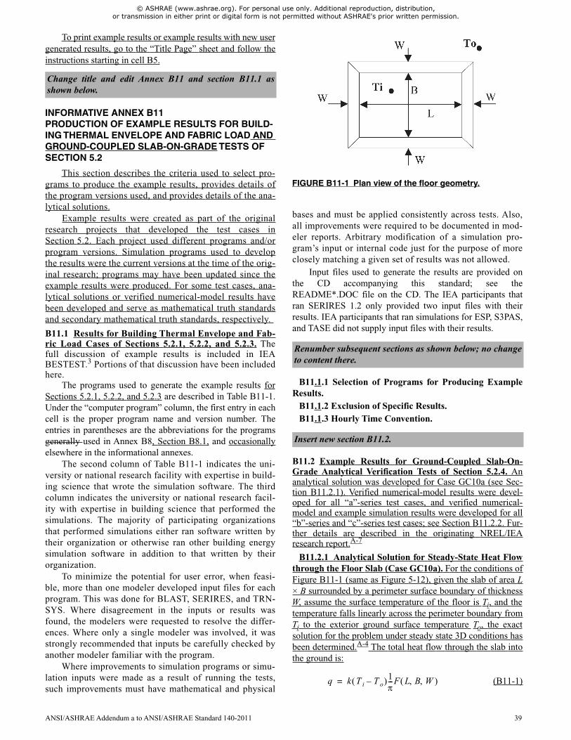
© ASHRAE (www.ashrae.org). For personal use only. Additional reproduction, distribution, or transmission in either print or digital form is not permitted without ASHRAE's prior written permission.
To print example results or example results with new usergenerated results, go to the “Title Page” sheet and follow theinstructions starting in cell B5.
INFORMATIVE ANNEX B11PRODUCTION OF EXAMPLE RESULTS FOR BUILD-ING THERMAL ENVELOPE AND FABRIC LOAD ANDGROUND-COUPLED SLAB-ON-GRADE TESTS OFSECTION 5.2
This section describes the criteria used to select pro-grams to produce the example results, provides details ofthe program versions used, and provides details of the ana-lytical solutions.
Example results were created as part of the originalresearch projects that developed the test cases inSection 5.2. Each project used different programs and/orprogram versions. Simulation programs used to developthe results were the current versions at the time of the orig-inal research; programs may have been updated since theexample results were produced. For some test cases, ana-lytical solutions or verified numerical-model results havebeen developed and serve as mathematical truth standardsand secondary mathematical truth standards, respectively.
B11.1 Results for Building Thermal Envelope and Fab-ric Load Cases of Sections 5.2.1, 5.2.2, and 5.2.3. Thefull discussion of example results is included in IEABESTEST.3 Portions of that discussion have been includedhere.
The programs used to generate the example results forSections 5.2.1, 5.2.2, and 5.2.3 are described in Table B11-1.Under the “computer program” column, the first entry in eachcell is the proper program name and version number. Theentries in parentheses are the abbreviations for the programsgenerally used in Annex B8, Section B8.1, and occasionallyelsewhere in the informational annexes.
The second column of Table B11-1 indicates the uni-versity or national research facility with expertise in build-ing science that wrote the simulation software. The thirdcolumn indicates the university or national research facil-ity with expertise in building science that performed thesimulations. The majority of participating organizationsthat performed simulations either ran software written bytheir organization or otherwise ran other building energysimulation software in addition to that written by theirorganization.
To minimize the potential for user error, when feasi-ble, more than one modeler developed input files for eachprogram. This was done for BLAST, SERIRES, and TRN-SYS. Where disagreement in the inputs or results wasfound, the modelers were requested to resolve the differ-ences. Where only a single modeler was involved, it wasstrongly recommended that inputs be carefully checked byanother modeler familiar with the program.
Where improvements to simulation programs or simu-lation inputs were made as a result of running the tests,such improvements must have mathematical and physical
bases and must be applied consistently across tests. Also,all improvements were required to be documented in mod-eler reports. Arbitrary modification of a simulation pro-gram’s input or internal code just for the purpose of moreclosely matching a given set of results was not allowed.
Input files used to generate the results are provided onthe CD accompanying this standard; see theREADME*.DOC file on the CD. The IEA participants thatran SERIRES 1.2 only provided two input files with theirresults. IEA participants that ran simulations for ESP, S3PAS,and TASE did not supply input files with their results.
B11.1.1 Selection of Programs for Producing ExampleResults.
B11.1.2 Exclusion of Specific Results.B11.1.3 Hourly Time Convention.
B11.2 Example Results for Ground-Coupled Slab-On-Grade Analytical Verification Tests of Section 5.2.4. Ananalytical solution was developed for Case GC10a (see Sec-tion B11.2.1). Verified numerical-model results were devel-oped for all “a”-series test cases, and verified numerical-model and example simulation results were developed for all“b”-series and “c”-series test cases; see Section B11.2.2. Fur-ther details are described in the originating NREL/IEAresearch report.A-7
B11.2.1 Analytical Solution for Steady-State Heat Flowthrough the Floor Slab (Case GC10a). For the conditions ofFigure B11-1 (same as Figure 5-12), given the slab of area L× B surrounded by a perimeter surface boundary of thicknessW, assume the surface temperature of the floor is Ti, and thetemperature falls linearly across the perimeter boundary fromTi to the exterior ground surface temperature To, the exactsolution for the problem under steady state 3D conditions hasbeen determined.A-4 The total heat flow through the slab intothe ground is:
(B11-1)
Change title and edit Annex B11 and section B11.1 asshown below.
Renumber subsequent sections as shown below; no changeto content there.
Insert new section B11.2.
FIGURE B11-1 Plan view of the floor geometry.
q k T i T o– 1---F L B W =
ANSI/ASHRAE Addendum a to ANSI/ASHRAE Standard 140-2011 39
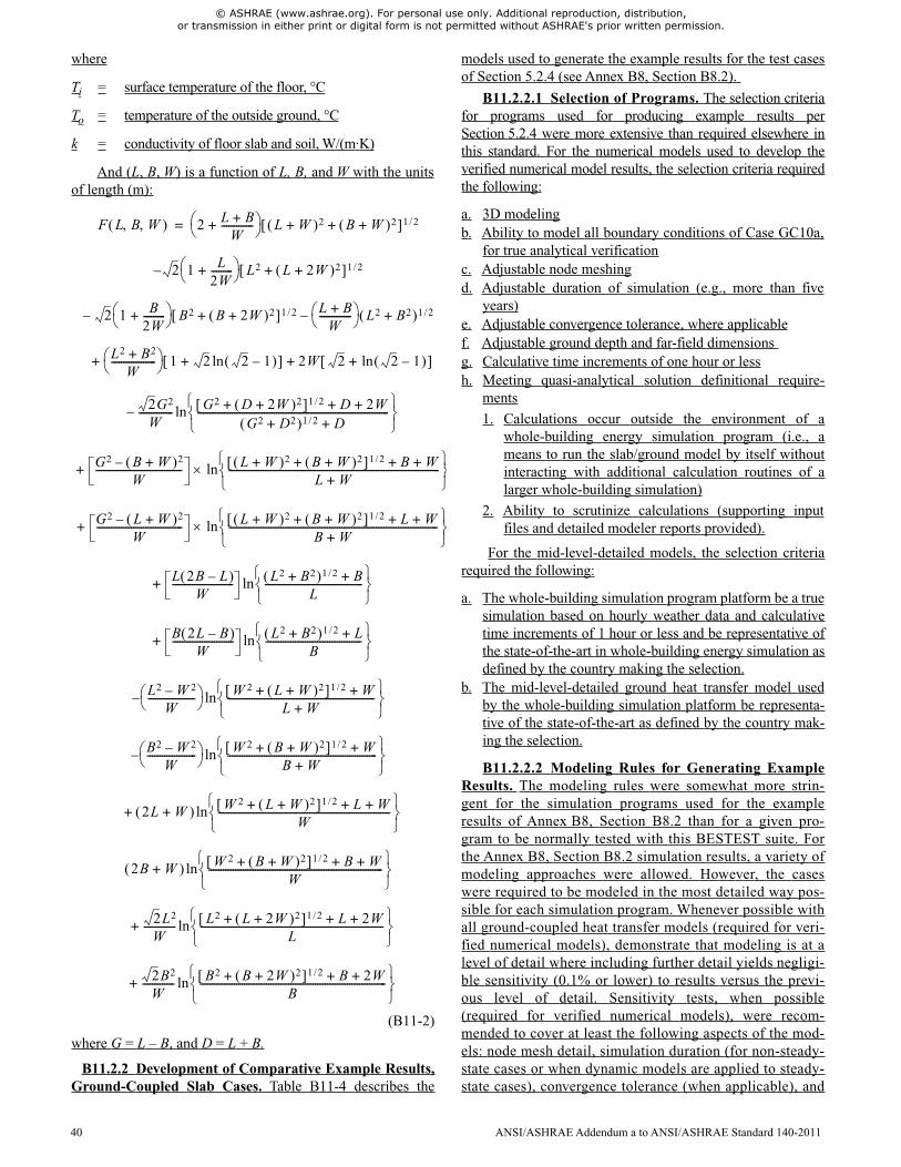
© ASHRAE (www.ashrae.org). For personal use only. Additional reproduction, distribution, or transmission in either print or digital form is not permitted without ASHRAE's prior written permission.
where
Ti = surface temperature of the floor, °C
To = temperature of the outside ground, °C
k = conductivity of floor slab and soil, W/(m·K)
And (L, B, W) is a function of L, B, and W with the unitsof length (m):
(B11-2)
where G = L – B, and D = L + B.
B11.2.2 Development of Comparative Example Results,Ground-Coupled Slab Cases. Table B11-4 describes the
models used to generate the example results for the test casesof Section 5.2.4 (see Annex B8, Section B8.2).
B11.2.2.1 Selection of Programs. The selection criteriafor programs used for producing example results perSection 5.2.4 were more extensive than required elsewhere inthis standard. For the numerical models used to develop theverified numerical model results, the selection criteria requiredthe following:
a. 3D modelingb. Ability to model all boundary conditions of Case GC10a,
for true analytical verificationc. Adjustable node meshingd. Adjustable duration of simulation (e.g., more than five
years)e. Adjustable convergence tolerance, where applicablef. Adjustable ground depth and far-field dimensionsg. Calculative time increments of one hour or lessh. Meeting quasi-analytical solution definitional require-
ments
1. Calculations occur outside the environment of awhole-building energy simulation program (i.e., ameans to run the slab/ground model by itself withoutinteracting with additional calculation routines of alarger whole-building simulation)
2. Ability to scrutinize calculations (supporting inputfiles and detailed modeler reports provided).
For the mid-level-detailed models, the selection criteriarequired the following:
a. The whole-building simulation program platform be a truesimulation based on hourly weather data and calculativetime increments of 1 hour or less and be representative ofthe state-of-the-art in whole-building energy simulation asdefined by the country making the selection.
b. The mid-level-detailed ground heat transfer model usedby the whole-building simulation platform be representa-tive of the state-of-the-art as defined by the country mak-ing the selection.
B11.2.2.2 Modeling Rules for Generating ExampleResults. The modeling rules were somewhat more strin-gent for the simulation programs used for the exampleresults of Annex B8, Section B8.2 than for a given pro-gram to be normally tested with this BESTEST suite. Forthe Annex B8, Section B8.2 simulation results, a variety ofmodeling approaches were allowed. However, the caseswere required to be modeled in the most detailed way pos-sible for each simulation program. Whenever possible withall ground-coupled heat transfer models (required for veri-fied numerical models), demonstrate that modeling is at alevel of detail where including further detail yields negligi-ble sensitivity (0.1% or lower) to results versus the previ-ous level of detail. Sensitivity tests, when possible(required for verified numerical models), were recom-mended to cover at least the following aspects of the mod-els: node mesh detail, simulation duration (for non-steady-state cases or when dynamic models are applied to steady-state cases), convergence tolerance (when applicable), and
F L B W 2 L B+W
-------------+ L W+ 2 B W+ 2+ 1 2/=
2 1 L2W---------+
L2 L 2W+ 2+ 1 2/–
2 1 B2W---------+
B2 B 2W+ 2+ 1 2/– L B+W
------------- L2 B2+ 1 2/–
L2 B2+W
------------------ + 1 2 2 1– ln+ 2W 2 2 1– ln+ +
2G2
W-------------- G2 D 2W+ 2+ 1 2/ D 2W+ +
G2 D2+ 1 2/ D+------------------------------------------------------------------------------
ln–
G2 B W+ 2–W
----------------------------------- L W+ 2 B W+ 2+ 1 2/ B W+ +L W+
--------------------------------------------------------------------------------------
ln+
G2 L W+ 2–W
----------------------------------- L W+ 2 B W+ 2+ 1 2/ L W+ +B W+
-------------------------------------------------------------------------------------
ln+
L 2B L– W
------------------------- L2 B2+ 1 2/ B+L
----------------------------------------
ln+
B 2L B– W
------------------------- L2 B2+ 1 2/ L+B
---------------------------------------
ln+
L2 W 2–W
------------------- W 2 L W+ 2+ 1 2/ W+
L W+------------------------------------------------------------
ln–
B2 W 2–W
-------------------- W 2 B W+ 2+ 1 2/ W+
B W+-------------------------------------------------------------
ln–
2L W+ W 2 L W+ 2+ 1 2/ L W+ +W
----------------------------------------------------------------------
ln+
2B W+ W 2 B W+ 2+ 1 2/ B W+ +W
-----------------------------------------------------------------------
ln
2L2
W------------- L2 L 2W+ 2+ 1 2/ L 2W+ +
L---------------------------------------------------------------------------
ln+
2B2
W------------- B2 B 2W+ 2+ 1 2/ B 2W+ +
B----------------------------------------------------------------------------
ln+
40 ANSI/ASHRAE Addendum a to ANSI/ASHRAE Standard 140-2011
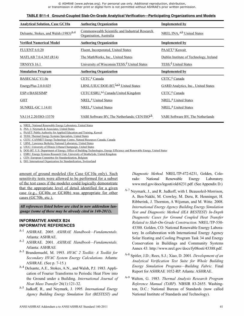
© ASHRAE (www.ashrae.org). For personal use only. Additional reproduction, distribution, or transmission in either print or digital form is not permitted without ASHRAE's prior written permission.
amount of ground modeled (for Case GC10a only). Suchsensitivity tests were allowed to be performed for a subsetof the test cases if the modeler could logically demonstratethat the appropriate level of detail identified for a givencase (e.g., GC40a or GC40b) was appropriate for othercases (GC70b, etc.).
INFORMATIVE ANNEX B24INFORMATIVE REFERENCESA-1 ASHRAE. 2005. ASHRAE Handbook—Fundamentals.
Atlanta: ASHRAE.A-2 ASHRAE. 2001. ASHRAE Handbook—Fundamentals.
Atlanta: ASHRAEA-3 Brandemuehl, M. 1993. HVAC 2 Toolkit: A Toolkit for
Secondary HVAC System Energy Calculations. Atlanta:ASHRAE. (See p. 7-15.)
A-4 Delsante, A.E., Stokes, A.N., and Walsh, P.J. 1983. Appli-cation of Fourier Transforms to Periodic Heat Flow intothe Ground under a Building. International Journal ofHeat Mass Transfer 26(1):121-32.
A-5 Judkoff, R., and Neymark, J. 1995. International EnergyAgency Building Energy Simulation Test (BESTEST) and
Diagnostic Method. NREL/TP-472-6231, Golden, Colo-rado: National Renewable Energy Laboratory.www.nrel.gov/docs/legosti/old/6231.pdf. (See Appendix D.)
A-7 Neymark, J., and R. Judkoff, with I. Beausoleil-Morrison,A. Ben-Nakhi, M. Crowley, M. Deru, R. Henninger, H.Ribberink, J. Thornton, A Wijsman, and M. Witte. 2008.International Energy Agency Building Energy SimulationTest and Diagnostic Method (IEA BESTEST) In-DepthDiagnostic Cases for Ground Coupled Heat TransferRelated to Slab-On-Grade Construction. NREL/TP-550-43388. Golden, CO: National Renewable Energy Labora-tory. In collaboration with International Energy AgencySolar Heating and Cooling Program Task 34 and EnergyConservation in Buildings and Community SystemsAnnex 43. http://www.nrel.gov/docs/fy08osti/43388.pdf.
A-8 Spitler, J.D.; Rees, S.J.; Xiao, D. 2001. Development of anAnalytical Verification Test Suite for Whole BuildingEnergy Simulation Programs—Building Fabric. FinalReport for ASHRAE 1052-RP. Atlanta: ASHRAE.
A-9 Walton, G. 1983. Thermal Analysis Research ProgramReference Manual (TARP). NBSIR 83-2655. Washing-ton, D.C.: National Bureau of Standards (now calledNational Institute of Standards and Technology).
TABLE B11-4 Ground-Coupled Slab-On-Grade Analytical Verification—Participating Organizations and Models
Analytical Solution, Case GC10a Authoring Organization Implemented by
Delsante, Stokes, and Walsh (1983)A-4 Commonwealth Scientific and Industrial ResearchOrganisation, Australia
NREL/JNA, a,b United States
Verified Numerical Model Authoring Organization Implemented by
FLUENT 6.0.20 Fluent, Incorporated, United States PAAET,c Kuwait
MATLAB 7.0.4.365 (R14) The MathWorks, Inc., United States Dublin Institute of Technology, Ireland
TRNSYS 16.1 University of Wisconsin/TESS,d United States TESS,d United States
Simulation Program Authoring Organization Implemented by
BASECALC V1.0e CETC,e Canada CETC,e Canada
EnergyPlus 2.0.0.025 LBNL/UIUC/DOE-BT,f,g,h United States GARD Analytics, Inc., United States
ESP-r/BASESIMP CETC/ESRU,e,i Canada/United Kingdom CETC,e Canada
GHT NREL,a United States NREL,a United States
SUNREL-GC 1.14.01 NREL,a United States NREL,a United States
VA114 2.20/ISO-13370 VABI Software BV, The Netherlands; CEN/ISOj,k VABI Software BV, The Netherlands
a. NREL: National Renewable Energy Laboratory, United Statesb. JNA: J. Neymark & Associates, United Statesc. PAAET: Public Authority for Applied Education and Training, Kuwaitd. TESS: Thermal Energy Systems Specialists, United Statese. CETC: CANMET Energy Technology Centre, Natural Resources Canada, Canadaf. LBNL: Lawrence Berkeley National Laboratory, United Statesg. UIUC: University of Illinois Urbana/Champaign, United Statesh. DOE-BT: U.S. Department of Energy, Office of Building Technologies, Energy Efficiency and Renewable Energy, United Statesi. ESRU: Energy Systems Research Unit, University of Strathclyde, United Kingdomj. CEN: European Committee for Standardization, Belgiumk. ISO: International Organization for Standardization, Switzerland
All references listed below are cited in new addendum lan-guage (some of these may be already cited in 140-2011).
ANSI/ASHRAE Addendum a to ANSI/ASHRAE Standard 140-2011 41

© ASHRAE (www.ashrae.org). For personal use only. Additional reproduction, distribution, or transmission in either print or digital form is not permitted without ASHRAE's prior written permission.

POLICY STATEMENT DEFINING ASHRAE’S CONCERNFOR THE ENVIRONMENTAL IMPACT OF ITS ACTIVITIES
ASHRAE is concerned with the impact of its members’ activities on both the indoor and outdoor environment. ASHRAE’smembers will strive to minimize any possible deleterious effect on the indoor and outdoor environment of the systems andcomponents in their responsibility while maximizing the beneficial effects these systems provide, consistent with acceptedstandards and the practical state of the art.
ASHRAE’s short-range goal is to ensure that the systems and components within its scope do not impact the indoor andoutdoor environment to a greater extent than specified by the standards and guidelines as established by itself and otherresponsible bodies.
As an ongoing goal, ASHRAE will, through its Standards Committee and extensive technical committee structure,continue to generate up-to-date standards and guidelines where appropriate and adopt, recommend, and promote those newand revised standards developed by other responsible organizations.
Through its Handbook, appropriate chapters will contain up-to-date standards and design considerations as the material issystematically revised.
ASHRAE will take the lead with respect to dissemination of environmental information of its primary interest and will seekout and disseminate information from other responsible organizations that is pertinent, as guides to updating standards andguidelines.
The effects of the design and selection of equipment and systems will be considered within the scope of the system’sintended use and expected misuse. The disposal of hazardous materials, if any, will also be considered.
ASHRAE’s primary concern for environmental impact will be at the site where equipment within ASHRAE’s scopeoperates. However, energy source selection and the possible environmental impact due to the energy source and energytransportation will be considered where possible. Recommendations concerning energy source selection should be made byits members.
© ASHRAE (www.ashrae.org). For personal use only. Additional reproduction, distribution, or transmission in either print or digital form is not permitted without ASHRAE's prior written permission.

ASHRAE · 1791 Tullie Circle NE · Atlanta, GA 30329 · www.ashrae.org
7/14