The Profits to Insider Trading:A Performance-Evaluation Perspective

Leslie A. JengBoston University School of Management

Andrew MetrickDepartment of Economics, Harvard University and NBER

Richard ZeckhauserJohn F. Kennedy School of Government, Harvard University and NBER

January 1999

We thank Mirium Avins, Keith Higgins, Inmoo Lee, Mike Pascutti, Jay Patel, Eric Sirri, and AndreiShleifer for helpful comments. We acknowledge financial support from Harvard Business School (Jeng)and the Herrnstein Fund (Metrick and Zeckhauser).

2

ABSTRACT

This paper estimates the profits to insiders when they trade their company's stock. We construct

a rolling “purchase portfolio” that holds all shares purchased by insiders over the previous year

and an analogous “sale portfolio” that holds all shares sold by insiders over the previous year.

We then analyze the returns to these value-weighted portfolios using performance-evaluation

methods. This approach allows us to study the returns to insider transactions beginning on the

day after their execution, and is free of the statistical difficulties that plague event studies on

long-horizon returns. Using a comprehensive sample of reported insider transactions from 1975-

1996, we find that the purchase portfolio earns abnormal returns of about 40 basis points per

month, with about one-sixth of these abnormal returns accruing within the first five days after the

initial transaction, and one-third within the first month. The sale portfolio does not earn abnormal

returns. Our portfolio-based approach also allows for straightforward decompositions of the

purchase and sale portfolios by various characteristics. We find that the abnormal returns to

insider trades in small firms are not significantly different from those in large firms, and that top

executives do not earn higher abnormal returns than do other insiders.

3

1. Introduction

When corporate insiders trade their company’s stock, how much do they profit? What

kinds of stocks offer the greatest profits? Are high-volume trades more profitable than low-

volume trades? What is the expected cost to “outsiders” due to possible transactions with

insiders?

In this paper, we answer these questions using a comprehensive sample of reported

insider transactions from 1975 to 1996. The principal innovation in our approach is the

construction of value-weighted portfolios comprised of all insider trades. This portfolio-based

approach applies performance-evaluation methods to analyze the returns of insiders’ trades from

the day they are executed. These methods provide answers to new questions and offers fresh

insights into old ones.

By law, corporate insiders must file monthly SEC reports about their trades in their

company’s stock, and these reports are quickly made public.1 This data on insider trading has

inspired a large academic literature that studies the cross-sectional variation of stock returns as a

function of insider-trading activity. Representative articles include Lorie and Niederhoffer

(1968), Jaffe (1974), Seyhun (1986) and (1998), Rozeff and Zaman (1988), Lin and Howe

(1990), and Lakonishok and Lee (1998).2 This literature focuses on the abnormal returns to

firms depending on the “intensity” of insiders’ purchases and sales over well-defined periods.

For example, a stock may be labeled an “insider buy” for a month if at least three insiders bought

the stock and no insiders sold it. Alternatively, the definition may rely on the net number of

shares purchased and sold by insiders during the month. We refer to such rules as “intensive-

1 Section 2 discusses the definition of a corporate insider, and the regulation and reporting requirements of theirtrades.2 A closely related literature that studies insiders’ ability to forecast the time-series of aggregate stock returns, atopic we do not discuss in this paper. See Seyhun (1988), (1992), and (1998), and Lakonishok and Lee (1998).

4

trading” criteria. These studies use a variety of intensive-trading criteria for many different

samples, and are nearly unanimous in the conclusion that stocks that are intensely bought tend to

outperform relevant benchmarks over a subsequent period, and that those that are intensely sold

tend to underperform. They provide mixed evidence on whether other investors can profit, after

transactions costs, by using the public information contained in the insider trading reports.

Seyhun (1998) summarizes this evidence and concludes that several different trading rules lead

to profits.

The research cited above can be interpreted as tests of both the “strong” and “semi-

strong” versions of the efficient-markets hypothesis. If, for example, intensively purchased

stocks earn abnormal returns, then this would be evidence against the strong form. If outsiders

can use the public filings of insiders to construct successful trading strategies, then this would be

evidence against the semi-strong form (Fama, 1971). While intensive-trading criteria illuminate

the efficient-markets hypothesis, the approach encounters two challenges. First, the requirement

that intensity be defined over some interval means that stocks are only classified after these

intervals end. Therefore, the returns on the days immediately following most trades are not

included in the analysis. Second, the use of individual stocks as the main unit of analysis makes

it impossible to determine a value-weighted return to all trades; the stocks with intensive buying

or selling activity may comprise a small or a large part of overall trading. Attempts to overcome

these challenges by using event-study methods on daily returns for all trades (Pascutti, 1996)

encounter statistical difficulties due to both cross-sectional correlation and biases in computing

long-run abnormal returns.3

3 See Barber and Lyon (1997), Barber, Lyon, and Tsai (1998), and Kothari and Warner (1997).

5

In this paper, we surmount these difficulties by adopting a value-weighted portfolio-

based approach. We imagine that all insider purchases are placed into a portfolio on the day that

they are made and held for exactly one year. This “purchase portfolio” is like a shadow mutual

fund “managed” by the combination of all insiders. Since the holdings in this portfolio are

weighted in proportion to the values of the underlying insider trades, the returns on the portfolio

would correspond to the value-weighted returns earned by all insider purchases over one year.

Similarly, we can imagine a “sale portfolio” comprised of all shares sold by insiders, with these

shares held in the portfolio for exactly one year.

We use these constructed purchase and sale portfolios to assess the timeliness of insider

transactions. For some purposes, we might prefer instead to calculate the actual profits that

insiders make from their purchases and sales. Unfortunately, this is not possible: we have no

way to determine the actual holding period for insider purchases. For sales, there may be no

equivalent to a holding period, since a restorative purchase may never be made. Bearing such

difficulties in mind, we employ a one-year holding period for the stocks that insiders buy, and

calculate hypothetical insider profits from purchases on this basis. Thus, we are arbitrarily

defining “profits” to be “abnormal returns earned in the one-year period from date of

acquisition”. We say that the purchase portfolio earns a profit if its returns exceed a relevant

benchmark portfolio; in this case insiders are profiting by being in their own stock instead of the

benchmark for the one-year period from date of acquisition. In parallel fashion, we say the sale

portfolio “profits” if its returns fall below those of its relevant benchmark portfolio; with the sale

portfolio, insiders are profiting by investing in the relevant benchmark instead of their own stock

for the one-year period following date of sale.

6

These constructed purchase and sale portfolios allow for a novel perspective on insider

profits, made possible by two useful methodological devices. First, daily updating of the

portfolios allows us to include all stocks’ immediate post-trade performances in the analysis.

Second, the returns to the purchase and sale portfolios can be analyzed using performance-

evaluation methods and are free of the statistical difficulties that plague long-horizon event

studies. Another advantage of the value-weighted portfolio approach is that it allows simple

decompositions of the portfolios by time horizon, firm characteristics, and trading volume. By

constructing subportfolios, we can obtain point estimates and standard errors for the abnormal

returns to value-weighted insider trades conditional on each of these elements.

Beyond the scientific benefits, our estimation of insider profits is also motivated by

policy concerns: What are the welfare implications of the profits to insider trading? There is a

range of opinion.4 Some laissez-faire observers believe that insider trading should be legal, and

that profits from it should be part of corporate compensation. At the opposite extreme, financial

Puritans would object to the insiders’ profits as unjust enrichment, even if there were no

consequences for market (or corporate) performance.5

Lying in between is the position of American regulators, whose principal concern must

be whether the playing field is level: Profitable insider trading is bad as a symptom of markets

that are unfair to the outside investor, who is trading at an informational disadvantage. This is

unfair in itself, and furthermore undermines outsiders’ confidence in such markets, diminishes

their willingness to trade, and thereby reduces liquidity and efficiency within financial markets.

The regulators’ market-performance concern depends on perceptions of market fairness, not

4 See Bainbridge (1998) for a survey of this debate.5 Their disapproval would not vanish, even if it could be demonstrated that insider trading brought significant netbenefits, say because it brought stock prices more firmly into alignment with appropriate values. Their historicalancestors objected to bear-baiting, not because of the suffering of the bear, but because of the pleasure of the people.

7

necessarily reality. It is virtually impossible for outsiders to assess their disadvantage in such

markets, absent the detailed analysis to which we now turn.

Two other studies employ variants of the portfolio approach used in our paper. Finnerty

(1976) uses the CAPM to evaluate the equally weighted returns to all insider trades in NYSE

stocks from 1969 to 1972. Though equal weighting is reasonable for his study, which is

motivated as a test of the strong form of market efficiency, it leaves open the same questions as

do studies based on intensive-trading criteria. Eckbo and Smith (1998) use performance-

evaluation methods on monthly data for the complete sample of value-weighted insider holdings

in Norway from 1985 to 1992. In contrast to the results on U.S. data, they find that insiders do

not earn abnormal returns. The difference between their results and those for the U.S. may stem

from differences in a variety of institutional and methodological sources. This is further

motivation for a study of insider trading in the U.S. using our portfolio approach.

Overall, our evidence shows that insiders profit from their purchases but not from their

sales. In raw returns, the purchase portfolio outperforms the market by about 7.4 percent per

year. Using several performance-evaluation methods, we find that about one-third of this

outperformance can be explained by insiders’ propensity to buy small stocks, “value” stocks, and

those with higher market betas. Across the different methods, the remaining abnormal

performance ranges between 37 and 47 basis points per month. These point estimates are similar

to those found in studies that use intensive-trading criteria. We find that about one-sixth of these

abnormal returns accrue within the first five days after the trade, one-third within the first month,

and three-quarters within the first six months.

Despite the economically significant profits to insider purchases, we find that

counterparties (“outsiders”) have little to fear from these reported transactions. Insider trades

8

make up but a tiny portion of the market. On a value-weighted basis, insider purchases make up

only about 0.03 percent of total market volume, so the expected “cost” to outsiders due to the

purchases of insiders is about 0.15 basis points per year.6

In raw returns, the sale portfolio has about the same performance as the value-weighted

market. Consistent with previous studies, we find that insiders tend to sell “growth” stocks that

have performed well in the recent past. When we use performance-evaluation methods and

control for this tendency, all methods yield abnormal returns that are both economically and

statistically insignificant. This result differs from the literature on insider trading, where most

studies find negative abnormal returns for stocks that are intensely sold by insiders. Our use of

value weighting, as opposed to some intensity measure, is the most likely cause of this

difference. We also document a significant positive abnormal return for the first five days after

sale transactions. We provide evidence to show that this anomaly is caused by market-

microstructure effects following high-volume sales.

Following our analysis of the purchase and sale portfolios, we look at the portfolios

decomposed along several dimensions: volume of the trade, size of the firm, insider’s position in

the firm, and whether the trade is executed directly for an insider or indirectly for another party.

These categories have previously been studied using intensive-trading criteria or event-study

methods to study market efficiency and to search for profitable trading rules based on the public

filings of insiders.7 Our goals are different. We ask, “how much do insiders profit?” from each

type of trade. We find that several of the results from intensive-trading studies do not extend to

our framework. For example, we find that insiders in small firms do not earn significantly

6 Details of this calculation are provided in Section 4.7 See Seyhun (1986) and (1998), Pascutti (1996), Lakonishok and Lee (1998).

9

higher profits than do insiders in large firms, and top executives do not earn significantly higher

profits than do other insiders.

The paper is organized as follows. Section 2 discusses the data and provides summary

statistics. Section 3 describes the three performance-evaluation methods we employ. Section 4

gives the performance-evaluation results for the main insider-purchase and insider-sale

portfolios. Section 5 analyzes decompositions of the purchase and sale portfolios by trade

volume, firm size, and the insider’s relationship to the firm. The conclusion summarizes our

results and puts them in context.

2. Data and Summary Statistics

The Securities and Exchange Act of 1934 (SEA) prohibits agents from trading securities

while in possession of material inside information. “Material insider information” can be loosely

defined as private information that a reasonable investor would consider important in the

decision to buy or sell a corporation's security.8 The enforcement of the SEA was substantially

strengthened by the Insider Trading Sanctions Act of 1984 and the Insider Trading Fraud

Enforcement Act of 1988. In response, many companies instituted their own restrictions on

insider trading to avoid any appearance of illegality.9 Do current restrictions and enforcement

measures prevent corporate insiders from trading profitably? That is the motivating question of

this paper.

To facilitate enforcement of the regulations, Section 16(a) of the SEA requires that open-

market trades by corporate insiders be reported to the Securities and Exchange Commission

(SEC) within ten days after the end of month in which they took place. For the purposes of this

8 For a detailed discussion of the SEA, see Bainbridge (1998).9 Jeng (1998).

10

reporting requirement, “corporate insiders” include officers with decision-making authority over

the operations of the company, all members of the board of directors, and beneficial owners of

more than ten percent of the company’s stock. These reports, filed on the SEC’s “Form 4”, are

the source of data for almost all of the empirical studies of insider trading.10 Our data is drawn

from these Form 4 filings for the period from January 1, 1975 to December 31, 1996. These

filings contain information about each transaction and about the insider’s relationship to the firm.

(See Appendix A for more information about Form 4.)

Our analysis focuses on open-market purchases and sales by officers and directors. We

exclude options exercises, private transactions, and all transactions by beneficial owners. The

resulting database contains 563,863 transactions from 1975 to 1996, of which 214,897 are

purchases and 348,966 are sales.11 Sales outnumber purchases particularly in later years when

option and stock awards began to become a significant part of officers’ and directors’

compensation; such awards do not show up as purchases, but they do show up as sales when the

positions are liquidated. The typical sale is substantially larger than the typical purchase, with

average dollar values of $136,260 per sale as compared with $35,580 per purchase.

On a value-weighted basis, what percentage of all trades are made by insiders? This

percentage is straightforward to calculate as the dollar volume of insider purchases and sales

divided by the dollar volume of all trades. We calculate these percentages separately each month

for both purchases and sales, and we plot the time-series of these percentages in Figure 1. Over

the whole sample period, the average monthly ratio of value-weighted insider sales to all trades

is 0.22 percent. Thus, an outsider making a purchase would expect 0.22 cents per dollar to be

10 Two exceptions are Meulbroek (1992), who studies illegal (and unreported) insider trading, and Gompers andLerner (1998), who study venture capital distributions.11 We performed several steps to purge the data of coding errors. See Appendix A.

11

with insiders. The average monthly ratio of insider purchases to all trades is 0.03 percent. Thus,

outsiders making sales would expect only 0.03 cents per dollar from insiders.

Many studies of insider trading show that insiders sell stocks after they rise and buy them

after they fall.12 We also see this in our sample, as Figure 2 illustrates. We calculated an

abnormal return for every trade on every day, where abnormal returns are defined as the stock’s

return minus the return on the value-weighted market (NYSE/AMEX/Nasdaq). Cumulative

abnormal returns (CARs) are measured relative to the trading day by adding the daily abnormal

returns for all intervening days. These CARs are then averaged across all firms and graphed in

the figure. Thus, this analysis equally weights all trades beginning on the day of their execution.

Figure 2 shows that, on average, an insider sale is preceded by a positive CAR of about

12 percent over the preceding 100 days, but has no noticeable CAR after the sale. Purchases are

preceded by a negative CAR of about two percent over the 100 days prior to the trade date, and

are followed by a positive CAR of about six percent over the subsequent 100 days.

The average CARs graphed in Figure 2 provide only a crude measure of the abnormal

returns of insider trades. Aside from the obvious difficulties of using the value-weighted market

as the expected-return proxy for all stocks, there are also statistical problems due to biases in the

computation of CARs and the cross-sectional dependence of the abnormal returns among

transactions of the same firm and across firms.13 We sidestep these problems by constructing

“purchase” and “sale” portfolios and analyzing their returns with performance-evaluation

methods. To construct the purchase portfolio, we “buy” all insider purchases at the closing

prices on the day of the actual trades.14 We then hold these shares in the portfolio for one year.

12 Seyhun (1986) and (1998), Lakonishok and Lee (1998), Rozeff and Zaman (1998).13See Barber and Lyon (1997), Kothari and Warner (1997), and Barber, Lyon, and Tsai (1998).14We use closing prices on the day of the trade rather than the actual transaction prices of the insider transactionbecause of concerns about errors in the reporting of transaction prices. Please see Appendix A for a completediscussion of this issue.

12

Thus, the purchase portfolio includes all shares purchased by insiders over the previous year.

Similarly, the sale portfolio contains all shares sold by insiders over the previous year.

Figure 3 plots the total market value of the purchase and sale portfolios as a fraction of

the overall market. The series begins on January 1, 1976, so that both the portfolios have a full

year of history at all times.15 As would be expected, the sale portfolio is always larger than the

purchase portfolio. With all sales held for one year after the insider transaction, the sale portfolio

averages about 0.11 percent of the market. It is largest in recent years and reaches a peak of 0.23

percent of the market in 1994. The size of the purchase portfolio averages about 0.02 percent of

the market and does not demonstrate any obvious pattern over time.

The purchase and sale portfolios are likely to differ along many dimensions. First, we

would expect to observe more insider sales than purchases, if only for diversification and

liquidity motives. High-ranking corporate officers typically have substantial human capital

invested in their firms and often have large holdings of corporate stock and options relative to

their wealth.16 In addition, much executive compensation comes in the form of stock and

options, and these additions to insiders’ personal portfolios will not show up in our database. In

fact, a value-weighted plot of option exercises (not shown here) shows a striking similarity to the

plot of sales given in Figure 1; such similarity would be expected if many sales are executed in

conjunction with option exercises. Overall, we would expect that insider purchases are more

likely than sales to be information-driven.

Second, the purchase and sale portfolios differ from each other and from the overall

market in their stock composition; insiders tend to trade in stocks that are smaller in market

15 After January 1, 1976, the purchase and sale portfolios will have a full year of transactions in them. During 1975,the portfolios will necessarily be truncated as of January 1, 1975. Therefore, for consistency, we begin all theanalyses of the purchase and sale portfolios on January 1, 1976, and refer to our sample as beginning on that date.16 Hall and Liebman (1998).

13

capitalization than the “average” stock, with this pattern more pronounced for purchases.17 As an

illustration, we compute the fraction of the purchase and sale portfolios made up by the largest

and smallest stocks and we compare these fractions with analogous fractions for the whole

market. These fractions are computed for July 1 of each year and then averaged across all years

from 1976 to 1996. We define the “largest” stocks as those with market equities above the cutoff

for the largest third of the stocks on the NYSE. Analogously, the “smallest” stocks are those

with market capitalizations below the cutoff for the smallest third. Using these cutoffs, we

classify all stocks traded on NYSE, AMEX, and Nasdaq. Naturally, the largest stocks comprise

a far larger component of the value of the overall market (83.1 percent) than the smallest stocks

(5.5 percent). In contrast, the sale portfolio derives only 38.0 percent of its value from the

largest stocks and 29.1 percent from the smallest stocks. The purchase portfolio has an even

more extreme tilt toward small stocks, with only 22.0 percent of its value from the largest stocks

and 41.2 percent from the smallest stocks.

Rozeff and Zaman (1998) and Lakonishok and Lee (1998) show that insiders tend to buy

“value” stocks and sell “growth” stocks, as defined by several different value and growth

measures. This pattern also emerges in our purchase and sale portfolios, and can be illustrated

with a portfolio decomposition similar to the one we did for size. On July 1 of each year, we

calculate a book-to-market (BM) ratio for all stocks using their book value for the most recent

fiscal year (from COMPUSTAT) divided by market value as of the previous December 31. We

then rank all NYSE stocks by their BM ratios and find the cutoffs for the highest third (“value”)

and the lowest third (“growth”), and we use these cutoffs to classify all stocks. Next, we

calculate the fractions of the purchase portfolio, sale portfolio, and overall market that fall into

the value and growth categories. These fractions are computed once per year and then averaged

17 Seyhun (1986) and Rozeff and Zaman (1988).

14

across all years from 1976 to 1996. Using these definitions, the overall market consists of 50.2

percent growth stocks and 20.3 percent value stocks (and 29.5 percent in between). Relative to

the market, the sale portfolio demonstrates a slight tilt toward growth stocks, with 52.8 percent

growth and 17.1 percent value. The purchase portfolio exhibits a strong value tilt, with an

average of 34.1 percent growth and 34.8 percent value.

What are the returns to the purchase and sale portfolios? Figure 4 plots the value over

time for a hypothetical investment of $1 on January 1, 1976. Consistent with the results of

Figure 2, the purchase portfolio outperforms the market, while the sale portfolio earns returns

very close to the market. The annualized returns are 23.0 percent for the purchase portfolio, 16.4

percent for the sale portfolio, and 15.6 percent for the market.18 Of course, simple comparisons

of portfolio returns to the market tell only part of the story. To learn more, we need to use

performance-evaluation methods and calculate abnormal returns. We turn to this task in the next

section.

3. Performance Evaluation of Insider Trades

In the section, we describe the performance-evaluation methods that we use to analyze

insider’s returns. Since there is no consensus on the “right” model of expected returns, we

employ three methods that have proved useful in similar studies. Our first method of

performance evaluation is the standard CAPM of Sharpe (1964) and Lintner (1965).

18 This calculation ignores transactions costs, a policy that we follow throughout the paper and one that is consistentwith our purposes. One could easily approximate the annual transactions costs for these portfolios by multiplyingportfolio turnover (100 percent, by construction) by an estimate of round trip transactions costs.

15

Method 1: CAPM

ti,

tRMRF

i

i

tf, R

ti,R εβα ++=− , (1)

where Ri,t is the return on insider portfolio i in month t, Rf,t is the risk-free return in month t, and

RMRFt is the month t value-weighted market return minus the risk-free rate. Here, αi can be

interpreted as the abnormal return to portfolio i. Although research over the past 20 years has

produced significant evidence against this unconditional version of the CAPM, it is still used for

performance evaluation, both by academics and practitioners.19 Thus, it provides a good starting

point for our analysis.

Method 2: 4-Factor Model

One problem for the unconditional CAPM is that it cannot explain differences in returns

for portfolios sorted by stock characteristics such as size, past returns (momentum), or measures

of “value” such as the price-to-earnings, cash-flow-to-price, and book-to-market ratios.20 Since

Section 2 presented evidence that the purchase and sale portfolios differ from the market along

size, momentum, and value dimensions, it is important that we adjust for these “strategies” in our

analysis. The 4-factor model of Carhart (1997) is ideally suited for this purpose and has proved

useful in several recent studies of performance evaluation.21 The model is estimated by

ti, tPR1

i,4 tHML

i,3 tSMB

i,2 tRMRF

i,1

i

tf, R

ti,R εββββα +++++=− , (2)

19 Examples of the CAPM's continuing role in performance evaluation are Malkiel (1995), Morningstar (1996), andShirk et al. (1997).20 See Basu (1977) (P/E ratio), Banz (1981) (size), Fama and French (1993) (size and book-to-market), Lakonishok,Shleifer and Vishny (1994) (several value measures), and Jegadeesh and Titman (1993) (momentum).21See Carhart (1997), Chevalier and Ellison (1999), Daniel et. al (1997), and Metrick (1999).

16

where Ri,t, Rf,t, and RMRFt are defined as in (1). The terms SMBt (small minus big), HMLt (high

minus low), and PR1t (previous one-year return) are the month t returns to zero-investment

factor-mimicking portfolios designed to capture size, book-to-market, and momentum effects,

respectively.22 While there is an ongoing debate about whether these factors are proxies for risk,

we take no position on this issue and simply view the 4-factor model as a method of performance

attribution. Thus, we interpret the estimated alphas as “abnormal returns” in excess of what

could have been achieved by passive zero-cost investments in the factors.

Table 1 summarizes the factor returns over the January 1976 to December 1996 sample

period. As would be expected, average returns are positive for all of the factors: 73 basis points

a month for RMRF, 25 for SMB, 39 for HML, and 87 for PR1. It is striking that the momentum

factor earns a higher average return than the market factor. Note that these factor returns ignore

the transactions costs from their underlying trading strategies; such transaction costs would be

considerable for the monthly turnover necessary for PR1. However, our insider purchase and

sale portfolios also ignore transactions costs, and thus it is reasonable to measure their

performance relative to costless strategies.

Method 3: Characteristic-Selectivity (CS) Measure

Our third measure of performance is the “characteristic-selectivity” (CS) measure

developed by Daniel et al. (1997). This method matches each insider transaction to a portfolio of

similar stocks, and then calculates an excess return relative to this portfolio on each day. This

approach takes advantage of the transactions nature of the data, which substantially increases the

22 This model extends the Fama-French (1993) 3-factor model with the addition of a momentum factor. For detailson the construction of the factors, see Fama and French (1993) and Carhart (1997). We are grateful to Mark Carhartfor providing the factor returns.

17

precision of abnormal return estimates under some circumstances.23 Though the procedure is

conceptually straightforward, it is notationally cumbersome. We describe the basic idea here and

cover the details in Appendix B.

To obtain the CS measure, we begin by constructing 125 “bins” through independent

5x5x5 sorts on size, book-to-market, and momentum quintiles. NYSE breakpoints are used for

size and book-to-market, and combined NYSE/AMEX/Nasdaq breakpoints are used for

momentum, with all NYSE/AMEX/Nasdaq stocks placed into quintiles on the basis of these

breakpoints. Size and book-to-market sorts are performed once per year (on July 1), while

momentum sorts are performed at the beginning of every month. Therefore, stocks can change

bins every month. The three characteristics serve an analogous role to the SMB, HML, and PR1

factors in the 4-factor model. In the CS approach, all stocks with the necessary data are allocated

to a bin, which we call its “matching bin”.24 Next, we calculate a daily value-weighted return for

each bin. Then, for each of our insider portfolios, the monthly measure of abnormal returns is

calculated as the return on a zero-investment portfolio that is long the insider portfolio and short

a portfolio constructed using equivalent weights in the matching bins.

We write Ri,t as the return to insider portfolio i in month t and Bin i,t as the return to the

matching bins of insider portfolio i in month t. Then, the abnormal return to portfolio i for that

month, CS i,t, is equal to the difference between these two returns: CS i,t = R i,t – Bin i,t. For the

252 months of the sample period, the overall performance measure, CS i is written as

23See Metrick (1999).24Since some stocks must be excluded from this analysis because of a failure to match, the returns on the purchaseand sale portfolios will be slightly different here than for the factor models. Appendix B, which discusses theseissues, shows that any potential biases are small.

18

In this setup, CS i is comparable to α i from the factor models. Its statistical significance can be

assessed by using the time-series standard error of CS i,t.

The next two sections show that these three methods provide very similar results for the

abnormal returns of insiders. There are additional methods, of course, that could be used to

analyze returns, but no single analysis could employ all of them.25 We have no reason to believe

that our results would be qualitatively different using other methods.

4. The Level and Timing of Insider Profits

A. Performance Evaluation of the Purchase and Sale Portfolios

This section applies each of the three performance-evaluation methods to the purchase

and sale portfolios. In discussing the results, we use “performance measure” and “abnormal

returns” as synonyms. The relationship of abnormal returns to “insider profits” are reversed

between the purchase and sale portfolios. Since the purchase portfolio holds the stocks that

insiders buy, a positive abnormal return implies positive insider profits. Conversely, since the

sale portfolio holds the stocks that insiders sell, a negative abnormal return implies positive

insider profits.

25 For example, we do not employ any conditional factor models such as in Eckbo and Smith’s (1998) study ofinsider trading in Norway. We believe that the CS approach addresses similar concerns as do conditional models,with the added advantage that it exploits the transactions nature of the data.

(3) 252

CS

96 Dec

76Jan t i,∑

=iCS

19

Table 2 gives the results for the purchase portfolio. Under the CAPM, the purchase

portfolio has a significant α of 47 basis points per month.26 The CAPM β is 1.14 and is

significantly greater than one. As we discussed in Section 2, insiders tend to purchase small

stocks, value stocks, and those with low momentum. This strategy is also evident in the factor

loadings (or “betas”) from the 4-factor model, given in the third column of the table: positive and

significant loadings on SMB and HML, and a negative and significant loading on PR1. In Table

1, we saw that the average returns are positive for all of these factors, so while the positive

loadings on SMB and HML explain some of the abnormal performance observed in the CAPM,

the negative loading on PR1 works in the opposite direction. Together, these factor loadings

account for less than one-quarter of the abnormal return from the CAPM, and the 4-factor model

α is a significant 37 basis points. Notice that the adjusted R2 for the 4-factor model is higher

than for the CAPM (.92 vs. .79), and this added explanatory power results in a relatively large

difference in the standard errors of the respective α estimates (16 vs. 11 basis points).

The CS measure for the purchase portfolio is similar to those for the CAPM and the 4-

factor model, with a significant estimate of 41 basis points. Since the CS measure is computed

using a completely different method than are the alphas in the factor models, the similarity in

results is reassuring. Taken together, the evidence from Table 2 shows that insiders earn

economically large abnormal returns from their purchases, with point estimates ranging between

37 and 47 basis points per month. These results are consistent with evidence from studies that

use intensive-trading criteria.

The results for the sales portfolio appear in Table 3. Here, all performance measures are

economically small and statistically insignificant. The CAPM α is –9 basis points with a

26 Unless otherwise noted, “significant” refers to statistical significance at the five-percent level.

20

standard error of 14 basis points. Recall that this portfolio is made up of insider sales, so

negative values of α indicate that insiders are “profiting” by selling stocks that subsequently

underperform; in this case, however, the profits are insignificant. The CAPM β of 1.30 is

significantly greater than even the CAPM β from the purchase portfolio and indicates that

insiders sell stocks with high fundamental risk. This high β estimate explains why the sale

portfolio can outperform the market in absolute terms (Figure 4), yet still earn negative abnormal

returns under the CAPM.

For the 4-factor model, the loadings for the sale portfolio are different from those found

for the purchase portfolio, with these differences consistent with our analysis in Section 2 and

with the results of Rozeff and Zaman (1998). The loading on HML is negative and significant,

suggesting a tilt toward growth stocks. The loading on SMB, while positive, is significantly

lower than for the purchase portfolio. Interestingly, the loading on PR1, while positive, is

economically small and statistically insignificant. Thus, even though insiders tend to sell stocks

that have recently increased in price, these stocks do not subsequently perform like other high-

momentum stocks. With these loadings, the 4-factor model yields a positive but insignificant α

of 5 basis points per month. For the CS measure, the point estimate is an insignificant 6 basis

points per month. Overall, there is no evidence that insiders earn abnormal returns in the sale

portfolio. This is different from the typical finding in studies that use intensive-trading criteria;

we reconcile this difference in Section 5.A.27

Overall, these results show that “outsiders” have little to fear from insiders, at least those

who report their trades. Consider an outsider contemplating the sale of a stock to gain liquidity.

27 An exception is Lakonishok and Lee (1998), who find that stocks sold “most intensively” by insiders do notunderperform.

21

It is possible that this sale would be made to an insider, and insider purchases earn abnormal

returns of about 500 basis points in the first year. However, since insiders purchase only about

0.03 percent of all stock (see Figure 1), her expected “costs” of trading against an insider are

only 0.15 basis points.28 Thus, for a $10,000 sale, she would be willing to pay about 15 cents to

ensure that the trade did not have an insider as counterparty. This amount drops nearly to zero if

the outsider were making a purchase from an insider. Although insiders make a much larger

proportion of all sales (0.15 percent) than purchases, than their abnormal returns on sales are

small or nonexistent. Of course, there may be particular types of stocks or trades that lead to

higher expected losses for outsiders. We deal with this issue further in Section 5.B.

B. The Timing of Insider’s Abnormal Returns

We can better understand the dynamics of abnormal returns through a time

decomposition of the purchase and sale portfolios. To illustrate this decomposition, consider the

purchase portfolio. Recall that this shadow portfolio holds all insider purchases, using closing

prices from their transaction dates, and keeps them in the portfolio for exactly one year. Now,

we parse this strategy into portfolios that hold insider purchases for different subperiods during

that year: day0-day5, day5-day21, day21-month6, and month6-year1. That is, when an insider

trade first occurs, it is placed into the first portfolio (day0-day5); then, at the end of day 5, the

purchase is removed from the first portfolio and placed into the second portfolio (day5-day21);

etc. The days here are “trading days”; thus 21 days is approximately 1 month. We follow the

same procedure to decompose the sale portfolio.

28 The calculation is 500 * .0003 = .15 basis points. To make this calculation, we assume that stocks sold toinsiders subsequently outperform stocks sold to non-insiders by 5 percent. We do not argue that the insider tradessomehow “cause” this edge in performance; rather, the point here is to provide another perspective on the expectedvalue of the insiders’ superior information.

22

Table 4 shows annualized returns for each of these portfolios. For purchases, the

annualized returns are higher than the market in each case. The day0-day5 portfolio, which

contains all stocks purchased in the previous five days, earns annualized returns of 57.6 percent.

Either insiders time their purchases well or the market is somehow finding out about these

purchases and reacting to them. Somewhat surprising, however, are the returns earned by the

day0-day5 sale portfolio. Since this portfolio holds stocks that insiders have sold over the

previous five days, the high returns suggest insiders lose money relative to the market for the

first five days after a sale.

For both purchases and sales, the same patterns over the first five days are repeated at

smaller magnitudes over the subsequent 16 days, as can be seen from the day5-day21 results.

After the first 21 days, purchases modestly outperform the market, whereas sales perform

similarly to the market. To give more precise statements about performance, we turn to the

performance-evaluation models.

Table 5 gives performance measures and standard errors for the day0-day5, day5-day21,

day21-month6, and month6-year1 purchase and sale portfolios. The top panel gives the CAPM

alphas, the middle panel gives the 4-factor alphas, and the bottom panel gives the CS measures.

The results confirm the significance of the patterns seen in Table 4. The day0-day5 purchase

portfolio has highly significant positive point estimates across all models; these estimates range

between 252 and 304 basis points per month. These returns illustrate the importance of using

daily data to evaluate insider performance; any study that starts on report dates or uses only

monthly data will miss this effect. These monthly abnormal returns translate into daily abnormal

returns of about 13 basis points, or about 65 basis points over five trading days. Whether this is

seen as economically “large” depends on the context. For example, the day0-day5 portfolio

23

completely turns over every five trading days, far more often than any of the other portfolios

studied in this paper. Assuming a one percent roundtrip transaction cost, the day0-day5 portfolio

would incur approximately 400 basis points in transactions costs per month. Thus, the abnormal

returns are not sufficient to allow a profitable trading strategy after transactions costs, even if

such a trading strategy were otherwise feasible.

The purchase portfolio continues to earn abnormal returns well beyond 5 days. The

day5-day21 portfolio earns significant abnormal returns of 129 basis points under the CAPM,

114 under the 4-factor model, and 136 for the CS measure. For most insider transactions, more

than 21 days pass before the transactions get reported and made public. The corresponding

estimates for the day21-month6 portfolio are 54 basis points for the CAPM, 29 for the 4-factor

model, and 36 for the CS measure. Of these three estimates, all but the 4-factor α are significant.

For the month6-year1 portfolio, all the point estimates are positive, but none is significant. The

point estimates from Table 5 enable us to approximately decompose the overall abnormal returns

to the purchase portfolio; using either the CS measure or the 4-factor α as our guide, about three-

quarters of the total one-year return comes in the first six months, one-third comes in the first

month, and one-sixth comes in the first five days.29

The most striking results of Table 5 are found for the day0-day5 sale portfolio. The

abnormal performance for this portfolio is positive and significant under all models, with point

estimates ranging between 80 and 96 basis points per month. This is approximately equivalent to

4 to 5 basis points per trading day. While these results are consistent with the returns presented

in Table 4, they still seem to be counterintuitive. Why would the stocks that insiders sell perform

29 The CS estimate for the overall purchase portfolio (Table 3) is 41 basis points per month, or approximately 492basis points per year. Since the point estimate for the month6-year1 portfolio is 19 basis points, we attribute 19 * 6= 114 of the total to the last six months. Similar calculations for the other horizons yield the estimates in the text.

24

so well over the subsequent five days? In section 5.A, we present evidence to show that these

short-horizon returns can be explained by the recovery from the price-depressing effect of high-

volume insider sales. That is, they are largely a market microstructure effect.

At longer horizons, sale portfolios fail to earn significant abnormal returns, with the

alphas and CS measures economically close to zero in most cases. Since our main sale portfolio,

analyzed in Section 4.A, holds stocks for one year, the positive abnormal returns earned in the

first five days do not noticeably change the overall results.

5. A Closer Look at Insider Profits

Thus far, we have confined our analysis to the aggregate purchase and sale portfolios. In

this section, we decompose the purchase and sale portfolios along several dimensions: volume of

the trade, size of the firm, insider’s position in the firm, and whether the trade is executed

directly for an insider or indirectly for another party. These subclasses have been studied using

intensive-trading criteria and/or event-study methods, techniques that could aid other investors in

forecasting future stock returns. Our analysis asks a different question – how much do insiders

profit in each type of trade? – and thus uses performance-evaluation methods on value-weighted

returns to answer it.

A. The Volume of a Trade

Are high-volume trades the most profitable? There are logical reasons to believe that the

highest-volume trades would reflect the strongest insider beliefs about corporate performance.

However, such trades may have other motivations. For example, insiders with sizeable corporate

holdings may make high-volume sales for diversification or liquidity purposes; such sales may

25

be motivated more by a desire to reduce risk or buy a new house than to increase returns. Also,

high-volume purchases may be related to a quest for corporate control and its non-pecuniary

benefits and may only partially be related to expectation of future returns. On a more cynical

note, one might believe that high-volume trades are more likely to be scrutinized by the SEC, so

that insiders who report trades on illegal “inside information” may wish to take lower profits, by

reducing or splintering trades, in order to reduce the probability of detection. These factors all

militate against finding the highest-volume trades to be the most profitable.

Past research has generally found a positive relationship between trade volume and

insider profits, although this relationship may break down for the highest-volume trades.30 In

this section, we reexamine this relationship through the lens of our portfolio-based approach.

Thus, we are able to extend the analysis to include the daily returns immediately following the

trades and analyzing these returns using performance-evaluation methods. Our approach also

allows for a time-decomposition of returns similar to Section 4.B; this decomposition can then

provide insight into the puzzling day0-day5 returns of the sale portfolio.

We begin by decomposing the purchase and sale portfolios by trade volume into “low-

volume”, “medium-volume”, and “high-volume” purchase and sale portfolios. To form these

portfolios, we first calculate the fraction of firm equity traded in each transaction. For example, a

purchase of 10,000 shares of a stock with 100 million shares outstanding would represent 0.01

percent of equity. Next, we sort all trades by these equity fractions, with purchases and sales

ranked separately. Based on these rankings, we divide purchases and sales into thirds: “low”,

medium”, and “high”. This yields cutoffs of 0.004 and 0.028 percent for the purchase portfolios,

30 See Seyhun (1986), Pascutti (1996), and Seyhun (1998). Jaffe (1974) finds no difference between overall testsand tests restricted to high-volume trades, but this may be due to his sample of only the largest NYSE firms, wherethe trade-volume effect has been found to be weakest (Seyhun (1998)).

26

and 0.010 and 0.048 percent for the sale portfolios. That is, all sales below 0.010 percent of firm

equity are classified as “low-volume”, above 0.048 percent are classified as “high-volume”, and

in-between as “medium-volume”.31 For our purposes, this procedure offers two advantages over

simpler classifications based on absolute measures such as the number of shares or dollars

traded. First, the absolute measures are highly correlated with firm size, and analyses based on

them might confound firm-size and trade-volume effects. Our use of equity fractions mitigates

this problem. Second, our approach increases the chance that trades with a large “market-

impact” are classified as “high-volume”.32 The importance of this property will be seen below.

The performance measures for the trade-volume portfolios are summarized in Table 6. To

compare estimates across the different portfolios, we estimate each model as a seemingly-

unrelated-regression (SUR) for the six decomposed purchase and sale portfolios; this framework

provides estimates for the covariance of the performance measures.33 The abnormal returns for

the high-volume and medium-volume purchase portfolios are economically large and statistically

significant on all tests, with magnitudes that are similar both to each other and to the overall

purchase portfolio. The low-volume purchase portfolio earns considerably lower abnormal

returns, although its 4-factor α and CS measure are still positive and significant. Using

covariance estimates from the SUR (not reported in Table 6), we find that the medium-volume

purchase portfolio achieves significantly higher performance measures on all three tests than

does the low-volume purchase portfolio. Differences between the high-volume and low-volume

31 We use the whole sample period to make these cutoffs, but this procedure – which looks forward as well asbackward – should not introduce any bias in this case.32 Trades could also be classified using dollar trading volume (rather than firm equity) in the denominator.Unfortunately, CRSP does not include volume data for Nasdaq firms until 1983, so this method is not feasible.33 In our case, the SUR approach yields exactly the same point estimates and standard errors as would separateestimations, and provides the covariance estimates necessary for our comparisons. Another method to compareperformance measures is to evaluate the returns to zero-investment strategies that are long in one portfolio (e.g. low-volume purchases) and short in another (e.g. medium-volume purchases). The SUR and zero-investmentapproaches are mathematically equivalent.

27

performance measures are significant at the ten-percent level on all tests. The overall results for

the purchase portfolios are consistent with Seyhun’s (1998) findings.

Performance measures for the sale portfolios are economically small and – with one

exception – not statistically significant. Under the CAPM, the low-volume sale portfolio earns

significant negative abnormal returns. The point estimate of -15 basis points is not economically

large, but it is relatively precisely estimated. This precision derives from the well-diversified

nature of the low-volume portfolio which, by construction, cannot be dominated by a small

number of positions. Note that there is no significant relationship between trade volume and

profits for insider sales on any of the tests: none of the performance measures is significantly

different from any other.

The results of Table 6 can help us to reconcile our overall findings with those of other

authors. Recall that our estimated abnormal returns for purchases (Table 2) are similar to those

found in other studies. Since the medium-volume and high-volume portfolios comprise two-

thirds of all trades and also represent the vast majority of traded shares and traded value, they

tend to dominate both our tests and the tests used by other authors. In contrast, the abnormal

returns for our sale portfolios are close to zero, while most other studies find negative abnormal

returns after sales. For tests based on the CAPM, these results are consistent with our findings.

The low- and medium-volume sale portfolios both have negative abnormal returns, and the

magnitude of these returns, while small, is similar to those found by other authors. The large-

trade sale portfolio, however, has slightly positive (but insignificant) abnormal returns, and it is

this portfolio that dominates our value-weighted analyses. Thus, a value-weighted approach

finds no abnormal returns for sales.

28

To shed light on the counterintuitive positive abnormal returns for the day0-day5 sale

portfolio, we perform the same time decomposition for each trade-volume portfolio that we did

in Section 4.B for the overall purchase and sale portfolios. Table 7 illustrates the returns to the

low-, medium-, and high-volume purchase and sale portfolios for the day0-day5 subperiod. The

table gives compelling evidence that the positive abnormal returns earned by the day0-day5 sale

portfolio are entirely driven by the highest-volume transactions. The high-volume sale portfolio

has positive and significant performance measures under all models, with point estimates ranging

between 130 and 144 basis points. Conversely, the performance measures for the low-volume

sale portfolio are negative and significant under all models; this is the direction that would be

expected when insiders make information-driven trades. Our hypothesis is that the high-volume

trades are driven primarily by liquidity or diversification motives, and that these big trades cause

downward price pressure, so that the day0-day5 abnormal returns are positive while the market

“bounces back” from this pressure.34 Since price pressure is small or nonexistent for medium-

and low-volume trades, we do not observe the same positive abnormal returns for those

portfolios. Since the high-volume trades dominate the value-weighted sale portfolio, they are

capable of driving the perverse short-run effect. This market-microstructure effect does not

prevent the high-volume purchase portfolio from earning positive returns; here, the information

component of these purchases overcomes any possible microstructure effect on prices.35

34 This kind of volume-based autocorrelation is documented in Conrad, Hameed, and Niden (1994).35 In addition, high-volume sales are bigger, on average, than high-volume purchases (see cutoffs given in Table 7),so the microstructure effect is likely to be smaller for the purchases than for sales.

29

B. Firm Size

Several studies that use intensive-trading criteria and event-study methods show that

insider trading is most profitable in small firms (Seyhun (1986) and (1998), Pascutti (1996),

Lakonishok and Lee (1998)). This empirical finding is consistent with intuition. The smaller the

firm, the easier it is for a single manager to know more relevant information. And since small

firms receive less attention than large firms do from Wall Street analysts, the smaller the firm,

the more likely that insiders hold an informational advantage over other market participants.

We analyze the relationship between firm size and insider returns by decomposing the

purchase and sale portfolios. At the beginning of each month, we divide the stocks traded on the

NYSE into thirds based on size (market value). We then use the cutoffs for these thirds to place

all NYSE/AMEX/Nasdaq stocks into one of three categories: “small-firm”, “medium-firm”, and

“large-firm”. Each insider transaction is then placed into a portfolio on the day of the trade

based on the size of the firm. This holding stays in the same portfolio for the full year, even if

the firm crosses a size cutoff. This procedure results in six portfolios (three for purchases and

three for sales).

We present the results in Table 8. As would be expected from the other results of this

paper, none of the sale portfolios earn significant abnormal returns under any of the methods.

The results are more interesting for the purchase portfolios. The small-firm purchase portfolio

earns significant abnormal returns under all three methods, with point estimates ranging between

31 and 51 basis points per month. For the other purchase portfolios, only the large-firm portfolio

earns significant abnormal returns on any test (32 basis points per month for the CS measure).

Nevertheless, the performance measures for the small-firm purchase portfolio are never

significantly different from the corresponding measures for either the medium- or large-firm

30

purchase portfolios.36 In fact, the biggest difference occurs under the CAPM (51 basis points for

small-firm purchases vs. 5 basis points for large-firm purchases), and some of this is certainly

attributable to the small-firm anomaly in the CAPM.37 Under the 4-factor model, the difference

in abnormal returns between the small- and large-firm purchase portfolios drops by half (relative

to the CAPM difference), and for the CS measure it disappears completely. Thus, and not

surprisingly, the marginal impact of firm size on insider profits is considerably smaller (or

nonexistent) once we control for size-related return anomalies.38 These results are not driven by

our use of only three size portfolios: there remains no significant difference between the

performance measures (4-factor alphas and CS measures) of the smallest and largest purchase

portfolios even if we use five or ten size groupings.39

While there is no significant difference in abnormal returns among the trade-size

portfolios, the probability of selling to an insider is much higher for small stocks (0.14 percent)

than for large ones (0.02 percent). Using the CS measure as our guide, an outsider making a sale

of a small stock faces an expected loss of 0.43 basis points due to the possibility he is trading

with an insider. While this is hardly monumental, it is approximately seven times higher than the

equivalent expected cost when trading in large stocks.

C. Insider’s Position within the Firm

Some insiders are more “inside” than others. The chief executive, for example, is likely

to have better information about the firm’s prospects than do lesser officers. Of course, since the

CEO’s trades are likely to be carefully scrutinized, both by shareholders and by regulators, he

36 This comparison uses covariances of the performance measures (not reported in the table) estimated by SUR.37 See Banz (1981) and Fama and French (1993).38 This same point is made by Rozeff and Zaman (1988), although their focus is on returns that can be earned byoutsiders following the publication of insider trading data.39 These results are available from the authors.

31

may be more reluctant to trade on his informational advantage. The net effect of these

considerations on the profitability of insider trading is an empirical question. Seyhun (1986 and

1998) analyzes the relationship between insiders’ positions in their firms and the profitability of

their trades, and concludes that there is an “information hierarchy”, with top executives at the

top, other officers in the middle, and directors at the bottom. In this section we study this

information hierarchy using performance-evaluation methods applied to value-weighted portfolio

returns.

We begin by decomposing the purchase and sale portfolios based on the job title of the

insider. “Top executives” are chief executives, chairmen of the board, and presidents.

“Officers” include all corporate officers except for top executives. “Directors” are members of

the corporate board who are not also officers. These categories do not overlap, and they cover

all trades in our sample.40 This decomposition results in three purchase portfolios and three sale

portfolios. The top-executive purchase portfolio constitutes 10.0 percent of the total purchase

portfolio, the officer-purchase portfolio 20.5 percent, and the director-purchase portfolio 69.5

percent. For sales, top-executives constitute 12.7 percent, officers 41.7 percent, and directors

45.6 percent.

The performance measures for these portfolios are summarized in Table 9. We estimate

each model as a SUR so that performance estimates can be compared across portfolios. None of

the sale portfolios earn significant abnormal returns on any of the tests. As usual, the purchase

portfolios offer more varied results. The officer-purchase and director-purchase portfolios have

significant abnormal returns under all tests, with point estimates close to those found for the

40 These definitions differ slightly from Seyhun’s (1998), which do allow for overlap. Some insiders do not fit intoany of these categories. We exclude them from the beginning; they are not represented in the purchase and saleportfolios. Please see Appendix A.

32

overall purchase portfolio. Surprisingly, the top-executive purchase portfolio does not earn

significant abnormal returns under any of the tests; however, while these point estimates are

always below those for the officer-purchase and director-purchase portfolios, they never differ

from them significantly. Thus, we cannot conclude that top executives do worse with their

purchases than do officers or directors.

The difference between equal- and value-weighted analyses allows us to reconcile our

results with Seyhun’s. The trades of top executives are about twice as big, on average, as those of

officers and directors. Also, top executives are responsible for a disproportionate number of the

very largest purchases. If the abnormal returns to purchases fall off for the very largest trades,

then all of the results are consistent.41 We do not adjust for the interaction of trade volume with

insider type because that is not the purpose of our analysis; if top executives trade in higher-

volume blocks than other insiders, we view this decision as a conscious choice of how they use

their information, and we are only interested in the net result on their profits.

The results of this section demonstrate why a value-weighted, portfolio-based analysis

provides an important perspective on insider trading. Seyhun’s results are important for

outsiders seeking to profit from the information content of insider trades; he shows that the

trades of top executives, whether equally-weighted or conditional on trade size, are more

informative about future returns than are the trades of other insiders. Our results are important

to regulators, and to outsiders who may be trading with insiders. We show that, unconditionally,

a dollar traded by a top executive earns no higher return than a dollar traded by another insider.

41 Seyhun’s (1998) analysis uses many categories of trade volume to search for the most informativetrades about future returns. He finds a concave relationship between trade volume and abnormal returns, withabnormal returns falling off for the very highest trades. Our analysis in Section 5.A. found medium-volumepurchases earning the same abnormal returns as large-volume purchases. This is consistent with the concaverelationship found by Seyhun.

33

D. Direct vs. Indirect Ownership of Shares

Insider’s holdings can be subdivided into two broad categories. “Direct” holdings are

held in the insider’s name. “Indirect” holdings are held in the name of another person, where the

corporate insider has a pecuniary interest, by reason of any contract, understanding, or

relationship.42 With the exception of Pascutti (1996), past studies of insider trading have not

distinguished between these two types of ownership.

In this section, we divide the sale and purchase portfolios into their direct and indirect

components. Thus, the direct-purchase portfolio contains all purchases for direct holdings made

over the previous year; the other portfolios are indirect-purchases, direct-sales, and indirect-sales.

The direct portfolios comprise the majority of both the purchase and sales portfolios, but the

indirect portfolios are still substantial, comprising 41.5 percent of the sale portfolio and 21.9

percent of the purchase portfolio.

It is not obvious what to expect for the relative performance of direct and indirect

portfolios. For direct trades, insiders are likely to exercise total discretionary control and keep

all the proceeds. In many indirect trades, insiders exercise considerably less discretion and have

smaller personal incentives. This suggests that direct trades would be more likely to reflect

insider information and yield higher profits.

However, insiders make many of their direct trades – particularly those of high volume –

to diversify their portfolios or gain more control of the corporation. Indirect trades, on the other

hand, are less likely to be driven by considerations of control or diversification, especially since

indirect holders usually do not have their human capital invested in the firm. Similarly,

purchases designed to increase control are probably more likely for a direct holding than for an

42See Goodman (1991).

34

indirect one. Since these considerations are stronger for high-volume transactions, they have the

potential to dominate a value-weighted analysis. This reasoning suggests that profits will be

higher for indirect trades than for direct ones.

Table 10 summarizes the evidence for the direct and indirect purchase and sale portfolios.

Once again, we estimate each model as a SUR so that the performance estimates can be

compared across portfolios. The CAPM α for the direct-purchase portfolio is 60 basis points; the

corresponding α for the indirect-purchase portfolio is 43 basis points. These point estimates are

significantly different from zero, but not from each other. The 4-factor alphas and CS measures

show a similar pattern. The direct-purchase portfolio earns a 4-factor α of 51 basis points and a

CS measure of 60 basis points, both of which are significant. The indirect-purchase portfolio

has a 4-factor α of 34 basis points and a CS measure of 31 basis points, but only the former

measure is significant. For each of the three tests, the performance measure for the direct-

purchase portfolio has a higher point estimate than the corresponding measure for the indirect-

purchase portfolio, but the difference is never significant. For the direct-sales and indirect-sales

portfolios, all of the performance measures are economically small and statistically insignificant.

Overall, there is no conclusive evidence of differential profits between direct and indirect trades.

6. Conclusion

There are three good reasons to study the profitability of trades by corporate insiders:

science, profit, and policy. Science examines the implications of the findings for market

efficiency. Profit hopes to develop optimal trading strategies, following the actions of insiders.

35

Policy seeks to determine the effectiveness of insider trading rules, and the implications of

insider profitability for both fairness and market performance.

Our analysis focused on science and policy. It began with the central question: How

much do insiders profit when they trade stock in their own firms? To address this question, we

employed performance-evaluation methods that analyze value-weighted portfolios comprised of

all insider trades. This approach – new to the insider trading literature – enables us to compute

any abnormal returns earned by insiders.

Insiders profit handsomely from their purchases, but not at all from their sales. This is not

surprising. Insider purchases likely reflect favorable information. Insider sales, by contrast, are

often made from shares received as part of executive compensation. Therefore, these sales may

be undertaken to gain liquidity or diversify holdings, implying little information content. Given

the sources and motivations of insiders’ sales, it is not surprising that their dollar volume is

nearly eight times that of purchases.

Insiders’ transactions differ from the market as a whole. Insiders disproportionately

purchase shares in small firms, value firms, and those that have recently underperformed. Their

sales are made mainly in growth firms that have experienced high recent returns. To correct for

differences in returns that may be driven entirely by these distinctive characteristics of insider

transactions, we calculated abnormal returns using three different performance-evaluation

methods. Under all three methods, the story is much the same. The abnormal returns to a value-

weighted portfolio of all insider purchases—holding positions for one year—are roughly 40 basis

points per month, an economically and statistically significant magnitude. The first five days

after purchase yield approximately one-sixth of the abnormal return, and one-third comes within

the first month. This evidence suggests that insider buyers have a good feel for near-term

36

developments within their firm, or that actions by others who follow their trades move the

market. None of our methods find that insider sales reap profits.

Our performance-evaluation methods can readily determine whether particular types of

trades do better or worse. Thus, we look at profitability by firm size, the dollar volume of the

transaction, and the insider’s position within the firm. We find that the trades of top executives

do no better than those of their less lofty peers. Similarly, firm size does not affect the

profitability of insider trading. However, low-volume purchases are less profitable than those of

higher-volume. We made no attempt to look at the potential for profitably following insiders’

trades; other methods are better suited to that investigation, and the prior literature has covered

them well.

What should policy makers think of our results? Surely insiders have valuable

information. If they do, only a Draconian regulatory system could prevent them from trading

profitably, and the evidence shows that the existing system does not. Policy makers can be

reassured, however, that the system is sufficiently effective -- presumably by holding down both

the volume and profitability of insider trades -- that outsiders are not significantly disadvantaged

when selling stock on the open market, and they are not disadvantaged at all when buying.

Inside purchases comprise just 0.02% of all purchases on the open market; on average, outsiders

lose just 15 cents on a $10,000 sale because an insider may be on the other side. But in circles

where this happy information is not widely known, investors with inflated perceptions of their

disadvantage may still be reluctant to trade.

Our principal accomplishment in this paper was to quantify the tilt in the playing field

enjoyed by insiders. Due to the disparity of numbers between insiders and outsiders, what

appears as an easy downward slide for the insiders produces an imperceptible upward tilt for

37

those who must trade against them. Inside traders are like ace handicappers at the racetrack.

They profit nicely, but only by imposing tiny losses on the masses. The question of fairness falls

to the eye of the beholder.

38

References

Bainbridge, Stephen, 1998, Insider Trading, forthcoming in the Encyclopedia of Law &Economics.

Banz, Rolf, 1981, The relation between return and market value of stocks, Journal of FinancialEconomics 38, 269-296.

Barber, Brad M. and John D. Lyon, 1997, Detecting long-run abnormal stock returns: Theempirical power and specification of test statistics, Journal of Financial Economics 43, 341-372.

Barber, Brad M., John D. Lyon, and Chih-Ling Tsai, 1999, Improved methods for tests of long-run abnormal stock returns, forthcoming in the Journal of Finance.

Barclay, Michael J. and Jerold B. Warner, 1993, Stealth trading and volatility: Which tradesmove prices? Journal of Financial Economics 34, 281-305.

Basu, Sanjoy, 1977, The investment performance of common stocks in relation to their price-to-earnings: A test of the efficient markets hypothesis, Journal of Finance 32, 663-682.

Brav, Alon and Paul Gompers, 1997, Myth or reality: The long-run underperformance of initialpublic offerings: Evidence from venture and nonventure capital-backed companies, Journal ofFinance 52, 1791-1822.

Carhart, Mark, 1997, On persistence in mutual fund performance, Journal of Finance 52, 57-82.

Chan, Louis K.C, Narasimhan Jegadeesh and Josef Lakonishok, 1995, Evaluating theperformance of value versus glamour stocks: The impact of selection bias, Journal of FinancialEconomics 38, 269-296.

Conrad, Jennifer, A. Hameed, and C. Niden, 1994, Volume and autocovariances in short-horizonindividual security returns, Journal of Finance 49, 1305-1329.

Daniel, Kent, Mark Grinblatt, Sheridan Titman, and Russ Wermers, 1997, Measuring mutualfund performance with characteristic based benchmarks, Journal of Finance 52, 1035-1058.

Eckbo, B. Espen and David C. Smith, 1998, The conditional performance of insider trades,Journal of Finance 53, 467-498.

Fama, Eugene F. and Kenneth R. French, 1993, Common risk factors in the returns on bonds andstocks, Journal of Financial Economics 33, 3-53.

Finnerty, J. E., 1976, Insiders and market efficiency, Journal of Finance 31, 1141-1148.

Gompers, Paul and Josh Lerner, 1998, Venture Capital Distributions: Short-Run and Long-RunReactions, Journal of Finance 53, 2161-2183.

39

Goodman, Amy L., 1991, A Practical Guide to Section 16: Reporting and Compliance, PrenticeHall Law & Business.

Jaffe, Jeffrey F., 1974, Special information and insider trading, Journal of Business 47, 410-428.

Jegadeesh, Narasimhan and Sheridan Titman, 1993, Returns to buying winners and sellinglosers: Implications for stock market efficiency, Journal of Finance 48, 65-91.

Jeng , Leslie A., 1998, Corporate insiders, market makers, and the window of opportunity,working paper, Boston University.

Hall, Brian and Jeffrey B. Liebman, 1998, Are CEOs really paid like bureaucrats?, TheQuarterly Journal of Economics 113, 653-692.

Kothari, S.P. and Jerold B. Warner, 1997, Measuring long-horizon security price performance,Journal of Financial Economics 43, 301-339.

Lakonishok, Josef and Inmoo Lee, 1998, Are insiders' trades informative?, NBER WorkingPaper No. 6656.

Lakonishok, Josef, Andrei Shleifer, and Robert Vishny, 1994, Contrarian investment,extrapolation, and risk, Journal of Finance 49, 1541-1578.

Lin, Ji-Chai and John S. Howe, 1990, Insider trading in the OTC market, Journal of Finance 45,1273-1284.

Lorie, James H., and Victor Niederhoffer, 1968, Predictive and statistical properties of insidertrading, Journal of Law and Economics 11, 35-53.

Loughran, Tim and Jay Ritter, 1995, The new issues puzzle, Journal of Finance 50, 23 - 52.

Malkiel, Burton, 1995, Returns from investing in mutual funds 1971 to 1991, Journal of Finance50, 549-572.

Metrick, Andrew, 1999, Performance evaluation with transactions data: The stock selection ofinvestment newsletters, forthcoming in the Journal of Finance.

Meulbroek, Lisa K., 1992, An empirical analysis of illegal insider trading, Journal of Finance47, 1661-1699.

Morningstar, 1996, Ascent database, April.

Pascutti, Michael J., 1996, Three Essays in Finance: Informed Trading on Nasdaq, ContrarianTrading by Insiders, and Swap Pricing, Ph.D. dissertation, Harvard University.

40

Rozeff, Michael S. and Mir A. Zaman, 1988, Market efficiency and insider trading: Newevidence, Journal of Business 61, 25-44.

Rozeff, Michael S. and Mir A. Zaman, 1998, Overreaction and insider trading: evidence fromgrowth and value portfolios, Journal of Finance 53, 701-716.

Seyhun, H. Nejat, 1986, Insiders' profits, costs of trading and market efficiency, Journal ofFinancial Economics 16, 189-212.

Seyhun, H. Nejat, 1988, The information content of aggregate insider trading, Journal ofBusiness 61, 1-24.

Seyhun, H. Nejat, 1992, Why does aggregate insider trading predict future stock returns?Quarterly Journal of Economics 107, 1303-1331.

Seyhun, H. Nejat, 1998, Investment Intelligence from Insider Trading, MIT Press.

Shirk, George S. III, Julie Cuenca and Greg Carlson, 1997, Platinum fund$, Mutual FundsOctober, 87.

Appendix A – Data Issues

Form 4 must be filed with the SEC within ten days following the end of each month in

which there is a change in direct or indirect insider ownership. Among the information required

on Form 4 are: name and address of reporting person, issuer name and ticker or trading symbol,

relationship of reporting person to the issuer (i.e., officer, director, etc.), filing date, type of

security traded, transaction date (month/day/year), transaction code (e.g., open-market

transaction, private transaction, transaction under an employee stock ownership plan), number of

equity securities traded, per share price of equity securities, ownership form (direct or indirect).43

We restrict our study to open-market transactions in equity securities that have data

available from the Center for Research in Securities Prices (CRSP). Over the January 1, 1975, to

December 31, 1996, sample period, there were 899,146 open-market transactions (386,102

43 Goodman (1991).

41

purchases and 513,044 sales). 44 Of this number, 17,340 (1.9 percent) have missing transaction

dates, leaving 881,806. We next purged duplicate transactions from this total. We defined a

duplicate as a transaction with identical data in all categories. We believe these duplicates can

occur for many innocuous reasons. This step removes 57,145 (6.5 percent) and leaves 824,661.

Prior to May 1991, Form 4 distinguished between open-market purchases and sales

(transaction codes P and S) and private transactions (transaction codes J and K). During this

period, open-market transactions outnumber private transactions by a ratio of about 11 to 1.

After May 1991, private transactions use the same codes as open-market transactions. Ideally,

we would exclude private transactions from our database; these transactions may take place with

restricted securities, the counterparty often knows he is trading with an insider, and the trade is

much more likely to be executed for liquidity or diversification motives than are open-market

transactions. Therefore, we do not include any private transactions prior to May 1991, and we

use several filter rules, discussed below, to eliminate the largest private transactions after this

date. These same filter rules also serve to purge the data of obvious coding errors.

Our first filter is to remove all transactions where the shares traded exceed trading

volume for that day. Since private transactions would not be included in the exchange traded

volume of the day, this filter is likely to catch many of the largest post-1991 private transactions.

This results in the loss of 4,030 transactions (0.5 percent) and leaves us with 820,631. Our

second filter purges all transactions whose prices fall outside the daily trading range reported on

CRSP. We call these “bad prices”. There are many reasons that bad prices can occur: a private

transaction may be executed outside of the range; the date, price, or transaction type may be

miscoded by the insider; input error may be made by the data provider, etc. The frequency of

44For transaction dates after May 1991, there are also some private transactions in our data set. Our methods fordisentangling these trades from open-market transactions are discussed below.

42

these problems, given below, is high enough to dissuade us from using the reported transaction

prices in our analysis. Furthermore, most of the reasons given for bad prices would also render

the transaction unsuitable for inclusion in the purchase and sale portfolios, even using the closing

prices.

Our analysis suggests that the majority of transactions with “bad prices” are due to

miscodes of the date (either by the insider or the data provider). Our procedure necessitates that

we first purge all transactions where CRSP provides no information on the trading range. This

results in a loss of 35,431 transactions (4.3 percent). Of the remaining 785,200 transactions,

221,337 (28.2 percent) have bad prices. To see how many of these may be due to simple

miscodes of the date (perhaps because the filing date is miscoded as the trading date), we

calculate a trading range beginning on the first day of the previous month and extending until the

last day of the current month. Out of 221,337 trades with bad prices, 163,141 (73.7 percent) fall

within this extended trading range. The remaining 58,196 trades with bad prices are likely to be

private transactions not caught in the previous filter, and other miscodes by the insider or the

data provider. Our final data set includes 563,863 transactions (214,897 purchases and 348,966

sales).

These filters have not caught all possible errors in the data. For example, any miscoded

dates that do not have bad prices will remain in the data set. Since such trades must necessarily

be in stocks with small price changes around the transactions, they are likely to bias our

abnormal returns toward zero. Our diagnostic tests suggest that the value-weighted fraction of

such bad trades is likely to be small and should not cause qualitative changes in our results.

Similarly, some private transactions will escape the filters. Since our filters would have caught

about 72 percent of the private transactions before May 1991, and the ratio of private

43

transactions to open-market transactions is small, we doubt that the remaining private

transactions would cause qualitative changes in our results.

Appendix B – The Characteristic-Selectivity (CS) Measure

This appendix provides the details for the computation of the CS measure described in

Section 3. This measure is based on the methodology of Daniel et al. (1997). For each insider

transaction portfolio, the monthly measure of abnormal returns is calculated as the return on a

zero-investment portfolio that is long in the insider transaction portfolio and short in a portfolio

constructed using equivalent weights in the matching bins. In effect, one just combines the

monthly abnormal returns for each stock in the portfolio.

The assumption underlying this model is that all stocks in the same bin have exactly the

same expected return. If this assumption is satisfied, then the performance measure will have a

zero expected return at all times. Thus, the insider portfolios that shift their portfolio

composition conditional on expected factor realizations will have no bias in their estimated

performance measure.

A more formal description of the methodology is:

d.day on i portfolioby sstock on placed weight ds(i),

W

and d,day on sstock tomatched bbin for return net db(s),

R

d,day on sstock for return net ds,

R

s,stock tomatched bbin :b(s)

i, portfolioby held s stocks all ofset the:is

month t,in d days all ofset the:td

=

=

=

∈∈

Using this notation, the CS measure for each month, CSi,t, is then calculated as

(4) ( ) ( )∏ ∑∏ ∑∈ ∈∈ ∈

∗+−

∗+=

td isb(s),ds(i),d

td iss,ds(i),dti, RW 1 RW 1 CS ,

44

where ( )∑ ∈∗

is s,ds(i),d RW is the actual net return for portfolio i on day d and ( )∑ ∈∗

is db(s),ds(i), RW

is the net return that would be achieved on day d if all funds were invested in the matching bins.

The CSi measure (Equation 3) is then calculated as the mean of the monthly CSi,t measures.

Not all stocks will be included in the CS calculation; if a stock cannot be matched to a

bin, then it is not included in the test. The two main reasons for a failure to match are, first,

insufficient past returns for a momentum calculation and, second, the absence of a book-equity

observation in COMPUSTAT. Both of these data requirements lead to new issues being deleted

from the portfolios. To the extent that new issues underperform similar stocks, this causes an

upward bias in the estimated selectivity performance measure.45 If such an upward bias exists, it

does not seem to have a significant effect on the results. For example, when we repeat the

CAPM and 4-factor tests of Tables 2 and 3 using returns calculated only from stocks that have

bin assignments, then the results are almost identical: the CAPM α is 45 basis points for

purchases (two points lower than the corresponding α of 47 basis points in Table 2) and –9 basis

points for sales (exactly the same as the corresponding α in Table 3); the 4-factor α is 42 basis

points for purchases (five points higher than the corresponding α of 37 basis points in Table 2)

and nine basis points for sales (four basis points higher than the corresponding α of five basis

points in Table 3).

45 See Loughran and Ritter (1995) and Brav and Gompers (1997) for evidence on the new-issues bias. On a “bin-adjusted” basis, Brav and Gompers’ (1997) work suggests that this bias should not be large. See also Chan,Jegadeesh, and Lakonishok (1995) for a discussion of the bias induced by omitting stocks that do not have data inCOMPUSTAT.

45

Figure 1

Percentage of Market Volume Traded by Insiders

This figure plots insiders’ purchases and sales as a percentage of market volume for each month of thesample period. The percentage is calculated as the total value in all securities of insider purchases (sales)for that month divided by the total value of all monthly trading on NYSE, AMEX, and Nasdaq. Theaverage percentages across the whole sample are 0.03 percent for purchases and 0.22 percent for sales.

0.00%

0.10%

0.20%

0.30%

0.40%

0.50%

0.60%

0.70%

0.80%

0.90%

7601

7701

7801

7901

8001

8101

8201

8301

8401

8501

8601

8701

8801

8901

9001

9101

9201

9301

9401

9501

9601

Date

Per

cen

tag

e

Purchase Percentage Sale Percentage

46

Figure 2

Cumulative Abnormal Returns Measured from the Date of Insider Transactions

This figure plots the average cumulative abnormal return (CAR) measured from the date of insiderpurchase and sale transactions. Daily abnormal returns are defined here as a stock’s return minus thevalue-weighted market return. These daily abnormal returns are calculated for the day of the transaction(day 0) and for each of the 100 days before and after the transaction. The CAR for day -t is the sum ofdaily abnormal returns beginning on day -t and ending on day 0. The CAR for day t is the sum of thedaily abnormal returns beginning on day 0 and ending on day t. This procedure yields a time-series ofCARs for each insider purchase and sale; these CARs are averaged across all purchases and sales toproduce the figure. The sample is for transactions from January 1, 1975 to December 31, 1996.

-15%

-10%

-5%

0%

5%

10%

-100 -9

0

-80

-70

-60

-50

-40

-30

-20

-10 0 10 20 30 40 50 60 70 80 90

100

Day

Purchase CAR Sale CAR

47

Figure 3

Insider Purchase and Sale Portfolios as a Percentage of Total Market Capitalization

This figure shows the percentage of the market held in our insider purchase and saleportfolios. The purchase (sale) portfolio includes all shares purchased (sold) by insidersover the previous year. On each day, we calculate the percentage of the total marketvalue (NYSE/AMEX/Nasdaq) held in each of these portfolios. Monthly percentages areexpressed as the mean of the daily percentages from that month; these monthlypercentages are then plotted in the figure. For the sample period of January 1, 1976 toDecember 31, 1996, the averages of these monthly percentages are 0.02 percent forpurchases and 0.11 percent for sales.

0.00%

0.05%

0.10%

0.15%

0.20%

0.25%

7601

7701

7801

7901

8001

8101

8201

8301

8401

8501

8601

8701

8801

8901

9001

9101

9201

9301

9401

9501

9601

Date

Purchase Sale

48

Figure 4

Returns to Purchase and Sale Portfolios

This figure plots the value of a hypothetical $1 investment on January 1, 1976, in thepurchase portfolio, sale portfolio, and the value-weighted market. The purchase (sale)portfolio includes all shares purchased (sold) by insiders over the previous year. Thevalue-weighted market includes all NYSE, AMEX, and Nasdaq firms. The annualizedreturns to these portfolios are 23.0 percent for purchases, 16.4 percent for sales, and 15.6percent for the value-weighted market.

0

10

20

30

40

50

60

70

80

7601

7612

7712

7812

7912

8012

8112

8212

8312

8412

8512

8612

8712

8812

8912

9012

9112

9212

9312

9412

9512

9612

Date

Purchase Sale Market

49

Table 1

Summary Statistics of Factor Returns

This table provides summary statistics for the factors used in the CAPM (equation 1) andthe 4-factor model (equation 2). These factors – RMRF, SMB, HML, and PR1 –represent the returns to zero-investment portfolios designed to capture market, size, book-to-market, and momentum effects, respectively. (Consult Fama and French (1993) andCarhart (1997) on the construction of these factors.) The sample is from January 1, 1976to December 31, 1996.

Factor Mean Std. Dev. Minimum Maximum

RMRF 0.73% 4.27 % - 22.77% 12.68 %

SMB 0.25 2.53 - 9.79 9.06

HML 0.39 2.53 - 8.49 8.92

PR1 0.87 2.81 - 10.65 10.02

50

Table 2

Performance-Evaluation Results for Purchase Portfolio

This table presents the performance-evaluation results for the purchase portfolio. The purchaseportfolio includes all shares purchased by insiders over the previous year. Column 2 gives the resultsfor the CAPM (equation 1). Column 3 gives the results for the 4-factor model (equation 2). Column4 gives the results for the CS measure (equation 3). For the factor models, α is the regressionintercept, and the next four rows give coefficients and standard errors (in parentheses) for theindependent variables: RMRF, SMB, HML, and PR1. These independent variables are the returns tozero-investment portfolios designed to capture market, size, book-to-market, and momentum effects,respectively. (Consult Fama and French (1993) and Carhart (1997) on the construction of thesefactors.) The symbols * and ** indicate two-tail significance at the five-percent level and at the one-percent level, respectively. The bottom row of the table provides the R2 for the factor regressions.The sample is from January 1, 1976 to December 31, 1996.

CAPM 4-Factor CS Measure

αα 0.0047**(0.0016)

0.0037**(0.0011)

RMRF 1.1418**(0.0370)

1.0980**(0.0272)

SMB 0.7379**(0.0416)

HML 0.1641**(0.0450)

PR1 -0.1273**(0.0380)

CS 0.0041**(0.0011)

R2 0.7919 0.9153

51

Table 3

Performance-Evaluation Results for Sale Portfolio

This table presents the performance-evaluation results for the sale portfolio. The saleportfolio includes all shares sold by insiders over the previous year. Column 2 gives theresults for the CAPM (equation 1). Column 3 gives the results for the 4-factor model(equation 2). Column 4 gives the results for the CS measure (equation 3). For the factormodels, α is the regression intercept, and the next four rows give coefficients and standarderrors (in parentheses) for the independent variables: RMRF, SMB, HML, and PR1. Theseindependent variables are the returns to zero-investment portfolios designed to capturemarket, size, book-to-market, and momentum effects, respectively. (Consult Fama andFrench (1993) and Carhart (1997) on the construction of these factors.) The symbols * and** indicate two-tail significance at the five-percent level and one-percent level, respectively.The bottom row of the table provides the R2 for the factor regressions. The sample is fromJanuary 1, 1976 to December 31, 1996.

CAPM 4-Factor CS Measure

αα -0.0009(0.0014)

0.0005(0.0010)

RMRF 1.2985**(0.0319)

1.1171**(0.0235)

SMB 0.5371**(0.0360)

HML -0.4074**(0.0391)

PR1 0.0219(0.0329)

CS 0.0006(0.0009)

R2 0.8690 0.9460

52

Table 4

Annualized Returns for Time Decompositions of the Purchase and Sale Portfolios

This table provides the annualized returns for decompositions of the purchase and saleportfolios into four holding periods: day0-day5, day5-day21, day21-month6, and month6-year1. At the close of trading on the day of an insider transaction, the purchase or sale isplaced into the day0-day5 portfolio; at the end of day 5, the trade is removed from theprevious portfolio and placed into the day5-day21 portfolio; etc. This decomposition isdone separately for purchases and sales. The sample is from January 1, 1976 toDecember 31, 1996. The bottom row shows the annualized return on the value-weightedmarket for the same sample period.

day0-day5 day5-day21 day21-month6 month6-year1

Purchase 57.6% 34.7% 23.2% 18.3%

Sale 28.9 18.9 15.3 16.6

Market 15.6% 15.6% 15.6% 15.6%

53

Table 5Performance-Evaluation Results for

Time Decompositions of the Purchase and Sale Portfolios

This table presents the performance-evaluation results for decompositions of the purchase and sale portfolios intofour holding periods: day0-day5, day5-day21, day21-month6, and month6-year1. At the close of trading on the daythat an insider transaction occurs, the purchase or sale is placed into the day0-day5 portfolio; at the end of day 5, thetrade is removed from the previous portfolio and placed into the day5-day21 portfolio; etc.This decomposition isdone separately for purchases and sales. The top of the chart shows the regression intercepts, α, from the CAPM(equation 1). The middle shows the regression intercepts, α, from the 4-factor model (equation 2). The bottomportion shows the CS measure (equation 3). Standard errors appear in parentheses. The symbols * and ** indicatetwo-tail significance at the five-percent level and one-percent level, respectively. The sample is from January 1,1976 to December 31, 1996.

Purchase SaleCAPMday0-day5 0.0269**

(0.0032)0.0080**

(0.0023)

day5-day21 0.0129**(0.0026)

0.0015(0.0021)

day21-month6 0.0054**(0.0020)

-0.0016(0.0017)

month6-year1 0.0019(0.0018)

-0.0003(0.0017)

4-Factor Modelday0-day5 0.0252**

(0.0032)0.0096**

(0.0022)

day5-day21 0.0114**(0.0026)

0.0010(0.0019)

day21-month6 0.0029(0.0016)

-0.0010(0.0014)

month6-year1 0.0008(0.0012)

0.0007(0.0013)

CS Measureday0-day5 0.0304**

(0.0031)0.0085**

(0.0020)

day5-day21 0.0136**(0.0025)

0.0031(0.0019)

day21-month6 0.0036*(0.0018)

-0.0001(0.0013)

month6-year1 0.0019(0.0014)

0.0016(0.0012)

54

Table 6

Performance-Evaluation Results for Trade-Volume Decompositions of the Purchase and Sale Portfolios

This table presents the performance-evaluation results for decompositions of the purchase and sale portfolios bytrade volume. To form our component portfolios, we first calculate the percentage of firm equity traded in eachtransaction. Next, we sort all trades by these equity percentages, with purchases and sales ranked separately. Basedon these rankings, we divide purchases and sales into thirds: “low-volume”, “medium-volume”, and “high-volume”.This yields cutoffs of 0.004 and 0.028 percent for the purchase thirds, and 0.010 and 0.048 percent for the salesthirds; i.e, all sales below 0.010 percent of firm equity are classified as low-volume, above 0.048 percent areclassified as high-volume, and in-between as medium-volume. The top of the chart shows the regression intercepts,α, from the CAPM (equation 1). The middle shows the regression intercepts, α, from the 4-factor model (equation2). The bottom portion shows the CS measure (equation 3). Standard errors appear in parentheses. The symbols *and ** indicate two-tail significance at the five-percent level and one-percent level, respectively. The sample is fromJanuary 1, 1976 to December 31, 1996.

Purchase SaleCAPMlow-volume 0.0010

(0.0006)-0.0015**(0.0007)

medium-volume 0.0049**(0.0012)

-0.0010(0.0012)

high-volume 0.0050**(0.0019)

0.0006(0.0017)

4-Factor Modellow-volume 0.0013*

(0.0006)0.0001

(0.0007)

medium-volume 0.0039**(0.0008)

0.0003(0.0009)

high-volume 0.0040*(0.0014)

0.0006(0.0011)

CS Measurelow-volume 0.0015**

(0.0005)0.0000

(0.0006)

medium-volume 0.0046**(0.0007)

0.0003(0.0009)

high-volume 0.0043**(0.0014)

0.0008(0.0011)

55

Table 7

Performance-Evaluation Results for Trade-VolumeDecompositions of the day0-day5 Purchase and Sale Portfolios

This table presents the performance-evaluation results for decompositions of the day0-day5 purchase and saleportfolios by trade volume. The day0-day5 purchase (sale) portfolio includes all shares purchased (sold) by insidersover the previous five days. To decompose these portfolios by trade volume, we first calculate the percentage offirm equity traded in each transaction. Next, we sort all trades by these equity percentages, with purchases and salesranked separately. Based on these rankings, we divide purchases and sales into thirds: “low-volume”, “medium-volume”, and “high-volume”. This yields cutoffs of 0.004 and 0.028 percent for the purchase thirds, and 0.010 and0.048 percent for the sales thirds; i.e, all sales below 0.010 percent of firm equity are classified as low-volume,above 0.048 percent are classified as high-volume, and in-between as medium-volume. The top of the chart showsthe regression intercepts, α, from the CAPM (equation 1). The middle shows the regression intercepts, α, from the4-factor model (equation 2). The bottom portion shows the CS measure (equation 3). Standard errors appear inparentheses. The symbols * and ** indicate two-tail significance at the five-percent level and one-percent level,respectively. The sample is from January 1, 1976 to December 31, 1996.

Purchase SaleCAPMlow-volume 0.0118**

(0.0019)-0.0057**(0.0018)

medium-volume 0.0252**(0.0026)

-0.0048(0.0024)

high-volume 0.0301**(0.0042)

0.0131**(0.0029)

4-Factor Modellow-volume 0.0112**

(0.0021)-0.0043*(0.0019)

medium-volume 0.0240**(0.0025)

-0.0035(0.0023)

high-volume 0.0278**(0.0042)

0.0144**(0.0027)

CS Measurelow-volume 0.0142**

(0.0020)-0.0035*(0.0013)

medium-volume 0.0283**(0.0030)

-0.0021(0.0023)

high-volume 0.0349**(0.0042)

0.0130**(0.0024)

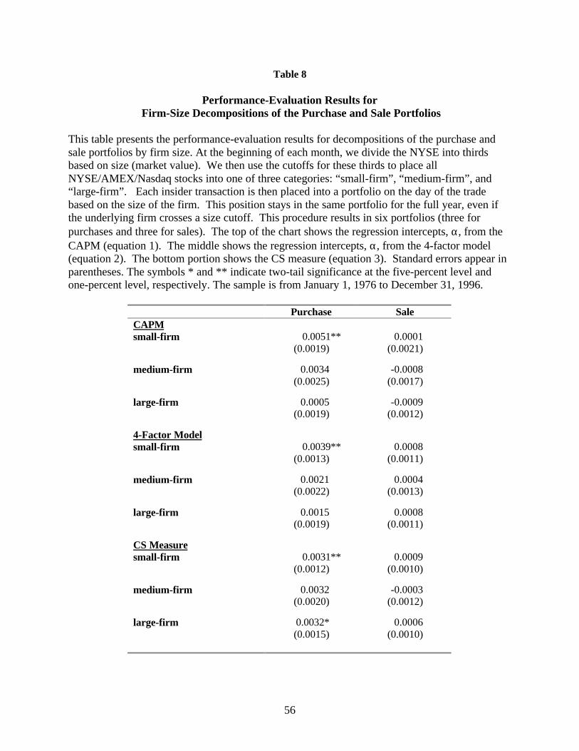
56

Table 8

Performance-Evaluation Results for Firm-Size Decompositions of the Purchase and Sale Portfolios

This table presents the performance-evaluation results for decompositions of the purchase andsale portfolios by firm size. At the beginning of each month, we divide the NYSE into thirdsbased on size (market value). We then use the cutoffs for these thirds to place allNYSE/AMEX/Nasdaq stocks into one of three categories: “small-firm”, “medium-firm”, and“large-firm”. Each insider transaction is then placed into a portfolio on the day of the tradebased on the size of the firm. This position stays in the same portfolio for the full year, even ifthe underlying firm crosses a size cutoff. This procedure results in six portfolios (three forpurchases and three for sales). The top of the chart shows the regression intercepts, α, from theCAPM (equation 1). The middle shows the regression intercepts, α, from the 4-factor model(equation 2). The bottom portion shows the CS measure (equation 3). Standard errors appear inparentheses. The symbols * and ** indicate two-tail significance at the five-percent level andone-percent level, respectively. The sample is from January 1, 1976 to December 31, 1996.

Purchase SaleCAPMsmall-firm 0.0051**

(0.0019)0.0001

(0.0021)

medium-firm 0.0034(0.0025)

-0.0008(0.0017)

large-firm 0.0005(0.0019)

-0.0009(0.0012)

4-Factor Modelsmall-firm 0.0039**

(0.0013)0.0008

(0.0011)

medium-firm 0.0021(0.0022)

0.0004(0.0013)

large-firm 0.0015(0.0019)

0.0008(0.0011)

CS Measuresmall-firm 0.0031**

(0.0012)0.0009

(0.0010)

medium-firm 0.0032(0.0020)

-0.0003(0.0012)

large-firm 0.0032*(0.0015)

0.0006(0.0010)

57

Table 9

Performance-Evaluation Results for Job-Title Decompositionsof the Purchase and Sale Portfolios

This table presents the performance-evaluation results for decompositions of the purchase andsale portfolios by job title of insider. “Top executives” are the subset of corporate officers thathold the title of chief executive, chairman of the board, or president. “Officers” include allcorporate officers except for top executives. “Directors” are members of the corporate boardwho do not also hold an officer title. These categories do not overlap and cover all trades in oursample. This decomposition results in three purchase portfolios and three sale portfolios. Thetop of the chart shows the regression intercepts, α, from the CAPM (equation 1). The middleshows the regression intercepts, α, from the 4-factor model (equation 2). The bottom portionshows the CS measure (equation 3). Standard errors appear in parentheses. The symbols * and** indicate two-tail significance at the five-percent level and one-percent level, respectively. Thesample is from January 1, 1976 to December 31, 1996.

Purchase SaleCAPMtop executive 0.0040

(0.0029)-0.0028

(0.0021)

officer 0.0053*(0.0021)

-0.0012(0.0014)

director 0.0044** (0.0017)

-0.0003(0.0014)

4-Factor Modeltop executive 0.0028

(0.0028)-0.0018

(0.0019)

officer 0.0054** (0.0018)

-0.0000(0.0010)

director 0.0030*(0.0013)

0.0010(0.0010)

CS Measuretop executive 0.0010

(0.0028)-0.0020

(0.0017)

officer 0.0046**(0.0017)

0.0005(0.0010)

director 0.0040**(0.0013)

0.0010(0.0010)

58

Table 10

Performance-Evaluation Results for Decompositions of thePurchase and Sale Portfolios between Direct and Indirect Trades

This table presents the performance-evaluation results for decompositions of the purchase andsale portfolios between direct and indirect trades. Securities owned directly are those held in thereporting person's name. Securities owned indirectly are those held in the name of anotherperson in which a reporting person has a pecuniary interest, by reason of any contract,understanding or relationship (including a family relationship or arrangement). The top of thechart shows the regression intercepts, α, from the CAPM (equation 1). The middle shows theregression intercepts, α, from the 4-factor model (equation 2). The bottom portion shows the CSmeasure (equation 3). Standard errors appear in parentheses. The symbols * and ** indicatetwo-tail significance at the five-percent level and one-percent level, respectively. The sample isfrom January 1, 1976 to December 31, 1996.

Purchase Sale

CAPMdirect 0.0060**

(0.0016)-0.0009(0.0014)

indirect 0.0043*(0.0019)

-0.0016(0.0016)

4-Factor Modeldirect 0.0051**

(0.0012)0.0007(0.0010)

indirect 0.0034*(0.0016)

-0.0008(0.0013)

CS Measuredirect 0.0060**

(0.0011)0.0008

(0.0010)

indirect 0.0031(0.0018)

-0.0002(0.0012)