MARINE ECOLOGY PROGRESS SERIESMar Ecol Prog Ser

Vol. 443: 39–50, 2011doi: 10.3354/meps09453

Published December 20

© Inter-Research 2011 · www.int-res.com*Email: s.chiswell@niwa.cri.nz

Annual cycles and spring blooms in phytoplankton:don’t abandon Sverdrup completely

Stephen M. Chiswell*

National Institute of Water & Atmospheric Research (NIWA) Ltd, Private Bag 14-901, Kilbirnie, Wellington, New Zealand

ABSTRACT: The critical-depth model for the onset of the spring phytoplankton bloom in theNorth Atlantic has recently been called into question by several researchers. The critical-depthmodel considers that the spring bloom starts when the mixed layer shoals to become shallowerthan a critical depth. Satellite and in situ measurements of chlorophyll are used here to show thatthe critical-depth model is indeed flawed. It is shown that the critical-depth model does not applyin the spring because the basic assumption of an upper layer that is well-mixed in plankton is notmet. Instead, the spring bloom forms in shallow near-surface layers that deepen with the onset ofthermal stratification. A stratification-onset model for the annual cycle in plankton is proposedthat adheres to the conventional idea that the spring bloom represents a change from a deep-mixed regime to a shallow light-driven regime, but where the upper layers are not well mixed inplankton in spring and so the critical-depth model does not apply. Ironically, perhaps, the critical-depth model applies in the autumn and winter when plankton are well-mixed to the seasonal thermocline, so that the critical-depth model can be used to determine whether net winter production is positive or negative.

KEY WORDS: Phytoplankton · Spring bloom · Annual cycle · Remote sensing · Critical-depthmodel

Resale or republication not permitted without written consent of the publisher

INTRODUCTION

The classic critical-depth model for the onset ofthe spring phytoplankton bloom in the NorthAtlantic (e.g. Siegel et al. 2002) has recently beencalled into question by Behrenfeld (2010, hereafterB2010), Boss & Behrenfeld (2010), and Taylor &Ferrari (2011). The critical-depth model is basedlargely on the work of Sverdrup (1953) and Gran& Braarud (1935), and considers that the springbloom begins when the mixed layer shoals to be -come shallower than a critical depth where the ver-tically integrated production equals the verticallyintegrated losses.

B2010 used satellite measurements of ocean colourand numerical model estimates of mixed-layer depthto find that in the North Atlantic, vertically integratedcarbon increases in winter even before the mixedlayer reaches its deepest value. B2010 suggests that

‘This finding strongly refutes the critical depth(model)’ (p. 980). Instead, B2010 proposes a dilution−recoupling model, where losses vary in time, and henotes ‘herein lies the crucial flaw in the critical depthhypothesis: Sverdrup assumed (losses) to be constantover time’. B2010 invites ‘other inter pretations’ of thedata.

Productivity is relatively high in subtropical waterseast of New Zealand (Fig. 1), and these waters alsoshow a spring bloom that has been considered to betriggered by shoaling of the seasonal thermocline(Murphy et al. 2001). Here, similar methods to thosedescribed by B2010 are used to compute the annualcycles in surface chlorophyll a (hereafter, chloro-phyll) and mixed-layer depth in the New Zealandregion. These cycles, along with data from a springbloom cruise made to the region, support a differentinterpretation for the breakdown of the critical-depthmodel than that suggested by B2010.

OPENPEN ACCESSCCESS

Mar Ecol Prog Ser 443: 39–50, 2011

The objective of this article is to present a concep-tual model of the annual cycle in primary productionin temperate waters where there is a spring bloom.In this ‘stratification-onset’ model, the annual cycleis controlled by the well-established mechanisms ofdeep mixing in the winter, and stratification inspring forming stable layers that allow near-surfaceproduction.

This article proceeds as follows. The next sectiondiscusses mixing and mixed-layer depths, and sum-marises the critical-depth model. The annual cyclesin surface chlorophyll and mixed-layer depth off theeast coast of New Zealand are then presented. This isfollowed by the results from the spring bloom cruiseand available historical hydrographic data. The strat-ification-onset model is then presented. It is sug-gested that while the dilution and recoupling notedby B2010 occur, they are incidental to the annual carbon cycle, rather than define it.

Before continuing, however, it is important to makeseveral comments. B2010 suggests that verticallyintegrated production may increase prior to thespring bloom, and states that ‘bloom initiation occursin the winter’ (p. 977). Thus, there is room for possi-ble confusion in the terminology related to the mean-ing of ‘bloom’. In this article, the term ‘spring bloom’is used to refer to the spring peak in surface chloro-phyll, regardless of whether or not it indicates thebeginning of the increase in total water-columnplankton.

It appears that Sverdrup (1953) has been largelymisinterpreted in the literature, and one has to distin-guish carefully between the concept of a criticaldepth and the idea that the spring bloom is triggeredwhen the surface mixed layer shoals to become shal-lower than this critical depth. Thus, in this article, theterm ‘Sverdrup (1953) hypothesis’ is used to referto the hypothesis that the critical depth is the levelabove which total production equals losses. The term‘critical-depth model’ is used to refer to the idea thatthe spring bloom is triggered when the thermoclineshoals above this critical depth.

The present study concentrates on chlorophyll, butit should be noted that chlorophyll can deviate frombiomass because of physiological changes in intra-cellular pigmentation (Kruskopf & Flynn 2006).

The mixed-layer depth is commonly defined to bethe depth at which density exceeds the surface valueby a specified difference, Δσ (e.g. de Boyer Montégutet al. 2004). B2010 used a mixed-layer depth definedby Δσ = 0.125 kg m−3 (M. J. Behrenfeld pers. comm.).This depth, which is denoted as Z0.125, is a good indicator of the depth of the seasonal thermocline.

MIXING AND MIXED-LAYER DEPTHS

It is important to recognise that apparently mixed(i.e. isopycnic) layers may not always be regions ofrapid vertical mixing (e.g. Brainerd & Gregg 1995).

40

Fig. 1. Mean surface chlo rophyll a (mg chl m−3), derived from 13 yr of SeaWiFS satellite observations of ocean colour. Blue dia-monds show locations of CTD casts made during the 2008 spring bloom cruise; grey diamonds show locations of historical CTDcasts (see ‘Results, Historical CTD data’). Inset shows locations of CTD casts made during the 2008 spring bloom cruise. Thesecasts were made tracking a drifter drogued at 15 m in order to follow an anti cyclonic eddy. During the cruise, the eddy made3 anticyclonic rotations, labelled I, II and III. Green, purple and red symbols, respectively, show CTD locations during these

three rotations

Chiswell: Annual cycles and spring blooms 41

The mixed layer is, by definition, the upper layer ofthe ocean that is well mixed in temperature and salin-ity (and thus density). However, at any given time,this layer may not be a region of active mixing. For ex-ample, at the end of winter, there may be a remnantdeep mixed layer that was formed by convective over-turn and/or winter storms, but with the cessation ofsurface cooling and a reduction of windstress, verticalmixing within this upper layer is considerably reducedcompared to the wintertime values.

If all horizontal processes are ignored, vertical mix-ing can be parameterised in terms of a vertical eddydiffusivity, K(z,t), and the growth rate of chlorophyll,C(z,t), at any level, z, and time, t, can be written (e.g.Huisman et al. 1999):

(1)

where μ(z,t) is the specific production rate (i.e. perunit chlorophyll), and l (z,t) is the specific loss rate,which represents all losses including respiration,grazing, parasitism and sinking. In general, Kdepends inversely on the stratification, becausestronger stratification will damp out vertical mixing(e.g. Jassby & Powell 1975).

The specific growth rate, q, in units (d−1) at anylevel is given by:

(2)

where .

Huisman & Sommeijer (2002) and Taylor & Ferrari(2011) argue that if K is below a critical value, thenvertical mixing may not be strong enough to mixplankton throughout the mixed layer, and there is thepotential for plankton to remain sufficiently high inthe water column so that blooms may developregardless of the depth of the mixed layer. Such lowrates of vertical mixing have been considered toaccount for observations of plankton blooms occur-ring even in the presence of deep mixed layers(Townsend et al. 1992). Conversely, when mixing isvery fast compared to plankton growth rates thenplankton are well mixed throughout the mixed layer.

It may be difficult in practice to determine from tem-perature and salinity profiles whether mixing is rapidor slow, but here it is argued that mixing generally re-sults from surface terms—convective overturn and/orwind stress. Thus, if the mixed layer is deepening, ac-tive mixing extends to the base of the mixed layer.Hence, it is assumed that when the seasonal thermo-cline is deepening, all tracers including chlorophyllare well mixed to the seasonal thermocline (at least to

a good approximation). However, when the seasonalthermocline is shoaling, one cannot make any state-ment about the strength of active mixing, andplankton may well be stratified in the mixed layer.

Sverdrup (1953)

Sverdrup (1953) assumed a nutrient-rich upperlayer with strong mixing so that phytoplankton arehomogenous throughout the upper layer. Heassumed specific production (μ) to be proportional tolight, specific losses (l) to be constant with depth, andthat light, I, is attenuated with depth, such that:

I (z) = I0exp(–kdz) (3)

where I0 is the surface irradiance and kd is the diffuseattenuation coefficient.

The critical-depth level (Zcr) is defined to be thedepth above which vertically integrated productionequals the vertically integrated losses, so that:

(4)

where the subscript 0 indicates surface values.Sverdrup (1953) defined the compensation ir -

radiance to be the irradiance at the depth where‘photosynthesis balances destruction by respiration’,although he used the term ‘respiration’ (p. 287) tomean all losses, including respiration, grazing andother losses such as sinking and parasitism. Becauseof his usage of the term respiration, there is thepotential for confusion, and here the term ‘equiva-lence irradiance’, Ieq, is introduced to mean the depthwhere production equals losses. The equivalenceirradiance occurs at the equivalence depth, Zeq.

With this substitution, the critical depth defined bySverdrup (1953) is given by:

(5)

If the mixed layer is shallower than Zcr there will benet positive growth in the mixed layer.

The assumption that losses are constant verticallywas made to make the integrations in Eq. (4) mathe-matically tractable. If losses are depth depen dent, thenEq. (4) can, in principle, be integrated numerically.

The critical-depth model

The critical-depth model stems from the Sverdrup(1953) hypothesis to suggest that, in the winter, the

μ0 00 0

exp( ) ( )− =∫ ∫k z z l zZ Z

d d dcr cr

11

0Zk Z k

I

Icrd cr d

eq− −( ) =exp( )

∂ − +∂

= ∂∂

∂∂

Ct

lz

K Cz

C( )μ

q z tCt

( , )nl ( )= ∂∂

q lC z

K Cz

= − + ∂∂

∂∂

μ 1

seasonal thermocline is deeper than the criticaldepth, so that net production is negative. The springbloom is initiated when the seasonal thermoclineshoals to become shallower than the critical depth.

It is worth emphasizing, that the critical depth (Zcr)depends on kd, Ieq, and I0. All of these variables willchange in time, so that the critical depth varies overthe year. As light increases, the equivalence and critical depths deepen. As grazing increases (i.e.losses increase), the equivalence and critical depthsshoal. However, time-varying critical depth does notchange the concept in the critical-depth model thatthe bloom is triggered by shoaling of the mixed layer.

METHODS

Satellite data from the sea-viewing wide field-of-view sensor (SeaWiFS) are available from the

NASA Ocean Color website (http://oceandata.sci.gsfc.nasa. gov/). Here, 8 d chlorophyll and photosyn-thetically available radiation (PAR) composite datamapped at a 9 km resolution from 1998 to 2010 wereused. These 9 km data were further averaged into 36by 36 km data using a median filter.

Meridional and zonal wind stress data were down-loaded from the National Centers for EnvironmentalPrediction (NCEP) Reanalysis Data (www.esrl.noaa.gov/psd/data/gridded/data.ncep.reanalysis.surfaceflux.html).

During the spring bloom cruise, conductivity- temperature-depth (CTD) measurements (e.g. Walk-ington & Chiswell 1993) were made following ananti cyclonic eddy off the east coast of New Zealandusing a drifter drogued at 15 m to determine the eddy location (Fig. 1). Chlorophyll derived from the CTDfluorometer was calibrated against extracted chloro-phyll from discrete water samples. Historical castsfrom the same region (Fig. 1) often had no calibrationdata, so nominal calibrations were applied.

Mixed-layer depths were calculated from CTD-derived profiles of density for 2 values of Δσ: 0.125and 0.025 kg m−3. These depths are denoted as Z0.125

and Z0.025, respectively. In the New Zealand region,the depths Z0.125 and Z0.025 correspond approximatelyto temperature differences of about 0.5 and 0.1°C,respectively.

Numerical values of mixed-layer depth, Z0.125, werecomputed from vertical temperature and salinity pro-files derived from a 14 yr hindcast provided by theBluelink project (Oke et al. 2005, 2008). This model isa 1/10° resolution, 47 layer z-level primitive equationmodel.

RESULTS

Satellite-derived annual cycles

Mean surface chlorophyll (Fig. 1) illustrates abroad band running across the Tasman Sea and eastof New Zealand at about 40 to 45° S. This is associ-ated with the Subtropical Front, which separateswaters of subtropical origin (STW) from those of sub-antarctic origin (Chiswell 2001). The spring bloomcruise took place well north of this front in subtropi-cal waters, characterised by surface salinity of ~35.3to 35.5 and surface temperature of ~20°C (summer)and ~14°C (winter). Mean surface chlorophyll for thespring bloom cruise location is 0.26 mg chl m−2.

Time series of satellite-derived surface chlorophylland numerical-model-derived mixed-layer depth

Mar Ecol Prog Ser 443: 39–50, 201142

J F M A M J J A S O N D J F M A M J J A S O N D J F M A M J J A S O N D

J F M A M J J A S O N D J F M A M J J A S O N D J F M A M J J A S O N D

J F M A M J J A S O N D J F M A M J J A S O N D J F M A M J J A S O N D

J F M A M J J A S O N D J F M A M J J A S O N D J F M A M J J A S O N D

1998 20001999

0

500

1000

2001 20032002

0

500

1000

2004 20062005

C0 ×

1000

(mg

chl m

−3 )

; Z0.

125

(m)

0

500

1000

2007 20092008

0

500

1000 Z0.125

C0

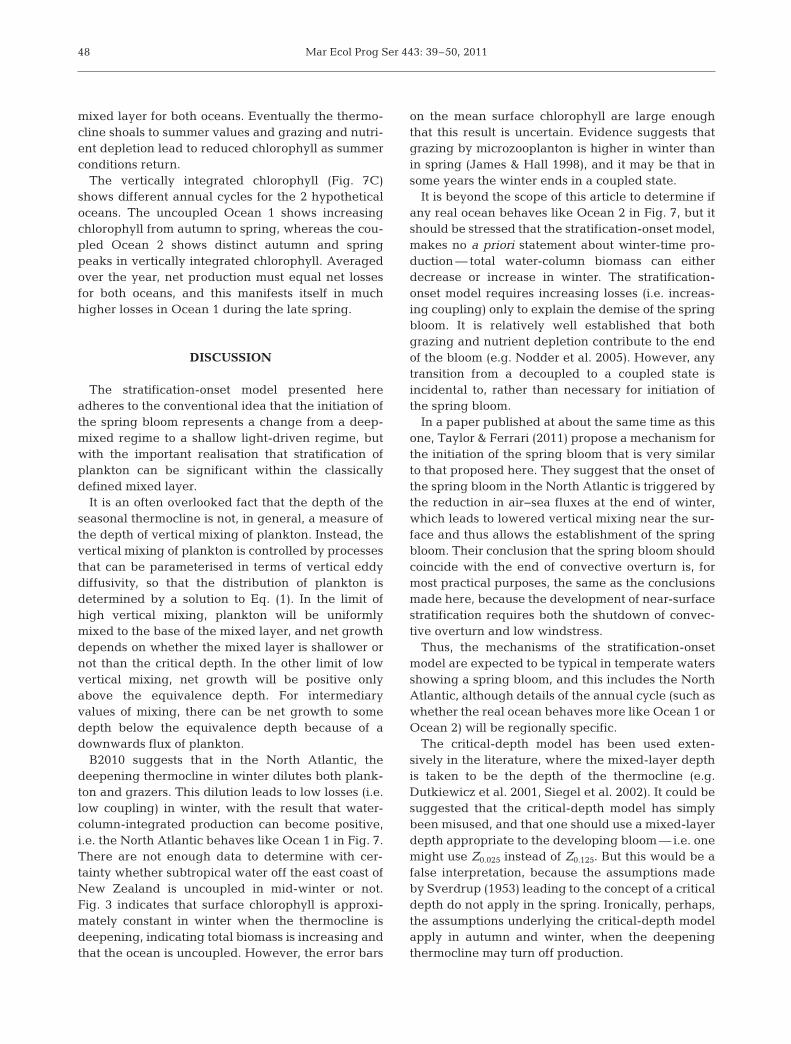
Fig. 2. Time series of satellite and numerical model productsfor the location of the 2008 spring bloom cruise (39.3° S,178.9° W). Surface chlorophyll (C0) was derived from SeaW-iFs data, and seasonal thermocline mixed-layer depth (Z0.125)was derived from a numerical model. Vertical line in 2008

indicates the start of the spring bloom cruise

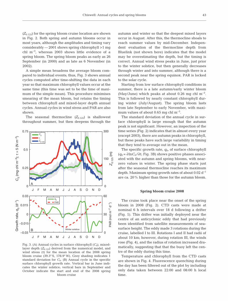
(Z0.125) for the spring bloom cruise location are shownin Fig. 2. Both spring and autumn blooms occur inmost years, although the amplitudes and timing varyconsiderably — 2001 shows spring chlorophyll >1 mgchl m−3, whereas 2003 shows little evidence of aspring bloom. The spring bloom peaks as early as 26September (in 2000) and as late as 6 November (in2002).

A simple mean broadens the average bloom com-pared to individual events; thus, Fig. 3 shows annualcycles computed after time-shifting the data in eachyear so that maximum chlorophyll values occur at thesame time (this time was set to be the time of maxi-mum of the simple mean). This procedure minimisessmearing of the mean bloom, but retains the timingbetween chlorophyll and mixed-layer depth annualcycles. Annual cycles in wind stress and PAR are alsoshown.

The seasonal thermocline (Z0.125) is shallowestthroughout summer, but then deepens through the

autumn and winter so that the deepest mixed layersoccur in August. After this, the thermocline shoals toreach summer values by mid-December. Indepen-dent evaluation of the thermocline depth fromBluelink (not shown here) indicates that the modelmay be overestimating the depth, but the timing iscorrect. Annual wind stress peaks in June, just priorto the winter solstice, but then generally decreasesthrough winter and into summer, although there is asecond peak near the spring equinox. PAR is lockedto the solar cycle.

Starting from low surface chlorophyll conditions insummer, there is a late autumn/early winter bloom(May/June) which peaks at about 0.26 mg chl m−3.This is followed by nearly constant chlorophyll dur-ing winter (July/August). The spring bloom lastsfrom late September to early November, with maxi-mum values of about 0.65 mg chl m−3.

The standard deviation of the annual cycle in sur-face chlorophyll is large enough that the autumnpeak is not significant. However, an inspection of thetime series (Fig. 2) indicates that in almost every year(except 2003), there are autumn peaks in chlorophyll,but these peaks have such large variability in timingthat they tend to average out in the mean.

The specific growth rate, q0, of surface chlorophyll(q0 = ∂ lnC0/∂t; Fig. 3B) shows positive phases associ-ated with the autumn and spring blooms, with near-zero values in winter. The spring phase starts justafter the seasonal thermocline reaches its maximumdepth. Maximum spring growth rates of about 0.02 d−1

are ca. 20% higher than those for the autumn bloom.

Spring bloom cruise 2008

The cruise took place near the onset of the springbloom in 2008 (Fig. 2). CTD casts were made at nominal 6 h intervals over 18 d following a drifter(Fig. 1). This drifter was initially deployed near thecentre of an anticyclonic eddy that had previouslybeen identified from satellite measurements of sea-surface height. The eddy made 3 rotations during thecruise, labelled I to III. Rotations I and II had radii ofabout 10 km; however, during rotation III, the windsrose (Fig. 4), and the radius of rotation increased dra-matically, suggesting that that the buoy left the cen-tre of the eddy during this time.

Temperature and chlorophyll from the CTD castsare shown in Fig. 4. Fluorescence quenching duringthe day has been filtered out of the plot by includingonly data taken between 22:00 and 08:00 h localtime.

Chiswell: Annual cycles and spring blooms 43C

0 (m

g ch

l m−

3 ); τ

× 5

(N m

−2 )

0

150

300

Z0.

125

(m)

0

0.25

0.5

0.75

J F M A M J J A S O N D

J F M A M J J A S O N D

Gro

wth

rat

e, q

0 (d

−1 )

0

30

60

PA

R (m

ol m

−2

d−

1 )

−0.03

−0.015

0

0.015

0.03

A

C0

τZ

0.125

Winter solsticeB

q0

PAR

Fig. 3. (A) Annual cycles in surface chlorophyll (C0), mixed-layer depth (Z0.125) derived from the numerical model, andwind stress (τ) for the mean location of the 2008 springbloom cruise (39.3° S, 178.9° W). Grey shading indicates 1standard deviation for C0. (B) Annual cycle in the specific surface chlorophyll growth rate. Vertical bar in June indi-cates the winter solstice; vertical bars in September andOctober indicate the start and end of the 2008 spring

bloom cruise

Mar Ecol Prog Ser 443: 39–50, 2011

For most of the experiment Z0.125 was about 300 to400 m deep — i.e. there was <0.5°C temperature dif-ference in the top 300 m, showing the presence ofdeep, nearly isothermal remnant winter mixed lay-ers. However, during the calm period starting 22September, heating of the upper water column led toa surface temperature rise of about 0.4°C over 3 d.This heating initially penetrated about 10 m, but asthe winds rose after 25 September, it was mixeddown to about 50 m. Stronger winds later mixed this

heat down further. During Rotation III, waters at from200 to 300 m depth show some warming, probablyassociated with the drifter (and hence CTD sampling)exiting the core of the eddy.

Surface chlorophyll was high at the beginning ofthe survey, decreased, and then rose to a local maximum on 25 September just before the windsincreased during Rotation II. However, the meanchlorophyll over the top 200 m (i.e. vertically aver-aged chlorophyll) was remarkably constant. The

depth of the chlorophyll layer, ZF, calcu-lated from the maximum vertical gradientin chlorophyll, was comparable to Z0.025

over much of the experiment, thus illus-trating that surface chlorophyll was con-tained in density layers that correspond totemperature differences of 0.1°C or less.The spring bloom was limited to theupper 150 m, even in the presence ofdeep remnant mixed layers.

The main conclusions derived from Fig.4 (i.e. that the spring bloom is limited tothe upper layers) can also be illustratedthrough vertical profiles of temperatureand chlorophyll made near midnight on 4successive nights from 24 to 28 Septem-ber during Rotation II (Fig. 5). All 4 castsshow shallow surface layers overlyingdeep remnant mixed layers extending tonearly 300 m. Chlorophyll is surfaceintensified and not homogeneous in thedeep remnant mixed layers. During thisperiod of time, increasing winds led todeepening of the near-surface layers(deepening Z0.025 from 11 to 33 m), whilethe thermocline shoaled slightly (Z0.125

shoaled from 313 to 304 m).

44

Fig. 4. Observations made during the 2008spring bloom cruise. Blue vertical bars indicatethe 3 rotations of the anticyclonic eddy trackedduring the cruise, labelled I, II and III (see‘Results, Spring bloom cruise 2008’). (A)Pseudo-wind stress from shipboard observa-tions. (B) Temperature section. Two estimatesof mixed-layer depth (Z0.125 and Z0.025) derivedfrom the CTD data are shown, as discussedin ’Results, Spring bloom cruise 2008’. (C) Surface (C0) and mean chlorophyll (C) de -rived from a CTD fluorometer over the upper200 m —surface chlorophyll has been dividedby 2. (D) Chlorophyll section derived from flu-orescence. The base of the chlorophyll layer,ZF, defined as the region of maximum vertical

gradient, is shown

Chiswell: Annual cycles and spring blooms

Historical CTD data

Twenty-eight historical temperature and chloro-phyll profiles from the region (Fig. 1) can be usedto illustrate the annual cycle (Fig. 6). Generally,summer profiles (December to February) show sub-surface chlorophyll peaking at the shallow seasonalthermocline, although 1 cast (31 December 1999)suggests that, even in summer, storms can lead todeep mixing. Autumn profiles (March to May)show a progression of deepening thermocline andin creased mixing of the upper layers so that chloro-phyll profiles progressively become more verticallymixed. Winter profiles (July to August) tend toshow deep (~300 m) isothermal layers and well-mixed chlorophyll. However, even in winter, therecan be some thermal stratification and gradients inthe chlorophyll (8 July 2006). Spring (September toOctober) profiles generally are consistent with the

2008 spring bloom cruise results, show-ing deep remnant winter layers andshallow surface stratification (i.e. deepZ0.125 but shallow Z0.025), with chloro-phyll trapped in the surface layers.

THE STRATIFICATION-ONSETMODEL

The observations that the spring bloomdoes not start until after the deepest mix-ing (Fig. 3), that it starts in the surfacelayers, and that it is not well mixed to theseasonal thermocline (Figs. 4 to 6) lead toa model for the seasonal cycle in plank-ton that incorporates conventional mech-anisms of nutrient and light availabilitycombined with mixing in the surfacemixed layer.

The basic tenets of the stratification-on-set model are that the seasonal thermo-cline is at its shallowest in summer be-cause of high summer solar insolation andrelatively light wind stress. Nutrients aredepleted in summer (e.g. Nodder et al.2005) so that production depends on thevertical flux of nutrients through the ther-mocline and chlorophyll shows a subsur-face maximum near the thermocline. Dur-ing autumn and winter, in creasedwindstress, combined with surface cool-ing and convective overturn, increasesurface-driven mixing, and this mixing

deepens the seasonal thermocline. Initially, this mix-ing leads to increased production in response to en -trainment of nutrients. The deepening thermoclineimplies that vertical mixing is rapid enough that alltracers including chlorophyll are well mixed (to agood approximation) above the thermocline. Thus, ifthe winter thermocline deepens below the criticaldepth, net production will become negative. Duringthe spring, however, windstress generally decreasesand convective overturn shuts down, so that deepmixing ceases. The seasonal thermocline representsthe base of the deep remnant mixed layer, but doesnot represent the depth of vertical mixing. Instead, shallow, weak (i.e. Δσ ≈ 0.025 kg m−3), surface mixedlayers may emerge soon after the thermoclinereaches its maximum depth. The spring bloom initi-ates near the surface in these layers, even if the ther-mocline is deeper than the critical depth. Productionin these surface layers will be positive, since they are

45

ZF

C (mg chl m−3)

Dep

th (m

Dep

th (m

24 Sep 2008 23:38 NZST

0 1 2 3 4 5 400

300

200

100

0

T (°C) C (mg chl m−3) T (°C)

C (mg chl m−3) T (°C) C (mg chl m−3) T (°C)

12 14 16

ZF

26 Sep 2008 00:17 NZST

0 1 2 3 4 5 400

300

200

100

0

12 14 16

26 Sep 2008 23:32 NZST

0 1 2 3 4 5 400

300

200

100

0

12 14 16

28 Sep 2008 02:39 NZST

0 1 2 3 4 5 400

300

200

100

0

12 14 16

Z0.025 Z0.025

Z0.025Z0.025

Z0.125Z0.125

Z0.125Z0.125

ZFZF

Fig. 5. Temperature (T) and chlorophyll (C) profiles from CTD casts madeapproximately 24 h apart during the spring bloom cruise (locations areshown in Fig. 1). Two estimates of mixed-layer depth (Z0.125 and Z0.025)

derived from the CTD data are shown. ZF: base of chlorophyll layer

almost certainly shallower than thecritical depth. In the deep remnantmixed layer below these surfacemixed layers, production will exceedlosses above the equivalence depth.This production will be mixed verti-cally by (weak) mixing, and chloro-phyll will show quasi-exponential de-crease with depth. Grazing in creasesrapidly after the initiation of thespring bloom, and this, together withconsumption of nutrients, leads to areturn to summer-time conditions.

Fig. 7 shows a schematic for thisstratification-onset model for 2 hypo-thetical oceans. These oceans aresimilar, except that Ocean 1 repre-sents an ocean where vertically inte-grated production exceeds lossesthroughout winter. Ocean 2 repre-sents an ocean which enters a loss-dominated phase in winter that couldbe due to either (or both) light limita-tion or high grazing. Under B2010’sdefinition, Ocean 1 is decoupled allwinter, whereas Ocean 2 becomescoupled in winter.

The thermocline depth shown inthe figure is based on Z0.125 for thespring bloom cruise location, i.e. itstiming is realistic for the New Zea -land region. The figure also showsthe equivalence and critical depths,Zeq and Zcr, for both hypotheticaloceans. These values were calculatedassuming a diffuse attenuation coeffi-cient, kd, equivalent to a 1% lightlevel of 50 m. The equivalence irradi-ance, Ieq, was set to 0.6 mol m−2 d−1 forOcean 1 and to 1.2 mol m−2 d−1 forOcean 2. These values are in therange of observed values (e.g. Siegelet al. 2002). Because of the exponen-tial nature of light extinction, there isonly a difference of about 5 m be-tween the equivalence depths for the2 oceans, but the critical depth forOcean 1 is >100 m deeper than thatfor Ocean 2 (Fig. 7A).

The middle panel of Fig. 7 illus-trates the growth of the water- column-integrated chlorophyll, r =∂Ctot /∂t, for the 2 oceans, where

Mar Ecol Prog Ser 443: 39–50, 201146D

epth

(m)

28 Jan 2007Z

0.125

0 10 20 30 400

200

002 Feb 2000

Z0.125

0 10 20 30

26 Feb 2005Z

0.125

0 10 20 30

02 Feb 2009Z

0.125

0 10 20 30

Dep

th (m

)

17 Mar 2002

Z0.125

0 10 20 30 400

200

007 Apr 2000

Z0.125

0 10 20 30

05 Apr 2001

Z0.125

0 10 20 30

14 Apr 2004

Z0.125

0 10 20 30

Dep

th (m

)

03 May 2005

Z0.125

0 10 20 30 400

200

030 May 2008

Z0.125

0 10 20 30

09 Jul 2001

Z0.125

0 10 20 30

Dep

th (m

)

26 Jul 2002

Z0.125

0 10 20 30 400

200

031 Jul 2004

Z0.125

0 10 20 30

08 Jul 2006

Z0.125

0 10 20 30

22 Aug 1998

Z0.125

0 10 20 30

04 Aug 2001

Z0.125

0 10 20 30

30 Sep 2001

Z0.125

0 10 20 30

Dep

th (m

)

02 Sep 2007

Z0.125

0 10 20 30 400

200

015 Sep 2008

Z0.125

0 10 20 30

Dep

th (m

)

01 Oct 2001

0 10 20 30 400

200

002 Oct 2005

Z0.125

0 10 20 30

01 Oct 2008

Z0.125

0 10 20 30

29 Oct 2009

Z0.125

0 10 20 30

20 Nov 2002

Z0.025

0 10 20 30

Dep

th (m

)

T; 10 × C

09 Nov 2003

Z0.125

0 10 20 30 400

200

0

05 Nov 2006

Z0.125

0 10 20 30

20 Dec 2001Z

0.125

0 10 20 30

31 Dec 1999

Z0.125

0 10 20 30

CT

Fig. 6. Temperature and chlorophyll profiles from the historic CTD casts (loca-tions are shown in Fig. 1). Chlorophyll has been scaled by 10. The profilesshow 2 estimates of mixed-layer depth, Z0.125 (horizontal lines) and Z0.025

(horizontal dashed lines) derived from the CTD data. The profiles are plotted according to the calendar day

Chiswell: Annual cycles and spring blooms

, and H is the water depth. The actualvalues of r are arbitrary — it is the relative magnitudeand sign in these values that differentiate Ocean 1from Ocean 2. The lower panel of Fig. 7 illustrates thetotal chlorophyll, Ctot, derived by integrating r froman initial value of 100 units.

Both oceans start summer with a subsurface maximum in chlorophyll, and the growth rates, r, arenegative because losses dominate production.

The seasonal thermocline starts to deepen in earlyautumn due to increased mixing, this time is denotedt1 in Fig. 7. Deepening of the thermocline continuesthrough the winter until the seasonal thermoclinereaches its maximum depth at time t3 (Fig. 7). Whilethe thermocline is deepening, all tracers are wellmixed to the thermocline depth. However, the 2hypothetical oceans behave quite differently duringthis time. For Ocean 1, the thermocline never deep-

ens below its critical depth. Thus, forthis uncoupled ocean, net production ispositive throughout autumn and winter,provided there are sufficient nutrients(although it is still possible that surfacechlorophyll decreases due to dilution asdiscussed by B2010). For Ocean 2, how-ever, the thermocline becomes deeperthan its critical depth at time t2, andthus, for this ocean, net production isnegative between t2 and t3 (Fig. 7B).

Once the thermocline ceases todeepen at time t3, emerging stratifica-tion in the surface layers and weak mix-ing there can support a spring bloom forboth oceans. The spring water columnis characterised by shallow weak mixedlayers lying over a remnant winter

C C zH

tot d= ∫0

47

J F M A M J J A S O N D

ZST

Summer Autumn Winter early Spring late Spring

Zcr

Zeq

Dep

th (m

)

Ocean 2Ocean 1

A 350

250

150

50

J F M A M J J A S O N D

Summer Autumn Winter early Spring late Spring

t1

t2

t3

t4

t5

B−10

−8

−6

−4

−2

0

2

4

J F M A M J J A S O N D

t1

t2

t3

t4

t5

Ocean 1

Ocean 1

Ocean 2

Ocean 2

C0

300

600

r =

∂C

tot/

∂tC

tot =

?∫ C

dz

Fig. 7. Schematic of the annual cycle in pri-mary production. (A) Depth of the seasonalthermocline, ZST (blue line), and equivalenceand critical depths, Zeq and Zcr, for 2 hypo-thetical oceans (red lines). Ocean 1 (dashedlines) is one where production exceeds lossesin winter, and Ocean 2 (solid line) is onewhere losses exceed production in winter. Insummer, chlorophyll (yellow profiles) showsa sub-surface maximum at ZST. Duringautumn and winter, chlorophyll is mixedthrough the mixed layer. If the thermocline isshallower than the critical depth (Zcr) net pro-duction can be positive given sufficient nutri-ents. In spring, the thermocline shoals due toerosion at the base of the mixed layer. Thespring chlorophyll bloom starts at the surfacewhen deep mixing ceases, allowing intermit-tent surface mixed layers to appear. By sum-mer, grazing and nutrient depletion reducechlorophyll in the upper layers. (B) Growthrates of vertically integrated production forOcean 1 and Ocean 2, see ‘The stratification-onset model’. (C) Vertically integrated bio-mass for Oceans 1 and 2, derived by integrat-ing the growth rates shown in Fig. 7B; t1 to t5

indicate various times in the annual cycle asdiscussed in the section ‘The stratification-

onset model’

Mar Ecol Prog Ser 443: 39–50, 201148

mixed layer for both oceans. Eventually the thermo-cline shoals to summer values and grazing and nutri-ent depletion lead to reduced chlorophyll as summerconditions return.

The vertically integrated chlorophyll (Fig. 7C)shows different annual cycles for the 2 hypotheticaloceans. The uncoupled Ocean 1 shows increasingchlorophyll from autumn to spring, whereas the cou-pled Ocean 2 shows distinct autumn and springpeaks in vertically integrated chlorophyll. Averagedover the year, net production must equal net lossesfor both oceans, and this manifests itself in muchhigher losses in Ocean 1 during the late spring.

DISCUSSION

The stratification-onset model presented hereadheres to the conventional idea that the initiation ofthe spring bloom represents a change from a deep-mixed regime to a shallow light-driven regime, butwith the important realisation that stratification ofplankton can be significant within the classicallydefined mixed layer.

It is an often overlooked fact that the depth of theseasonal thermocline is not, in general, a measure ofthe depth of vertical mixing of plankton. Instead, thevertical mixing of plankton is controlled by processesthat can be parameterised in terms of vertical eddydiffusivity, so that the distribution of plankton isdetermined by a solution to Eq. (1). In the limit ofhigh vertical mixing, plankton will be uniformlymixed to the base of the mixed layer, and net growthdepends on whether the mixed layer is shallower ornot than the critical depth. In the other limit of lowvertical mixing, net growth will be positive onlyabove the equivalence depth. For intermediary values of mixing, there can be net growth to somedepth below the equivalence depth because of adownwards flux of plankton.

B2010 suggests that in the North Atlantic, thedeepening thermocline in winter dilutes both plank-ton and grazers. This dilution leads to low losses (i.e.low coupling) in winter, with the result that water-column-integrated production can become positive,i.e. the North Atlantic behaves like Ocean 1 in Fig. 7.There are not enough data to determine with cer-tainty whether subtropical water off the east coast ofNew Zealand is uncoupled in mid-winter or not.Fig. 3 indicates that surface chlorophyll is approxi-mately constant in winter when the thermocline isdeepening, indicating total biomass is increasing andthat the ocean is uncoupled. However, the error bars

on the mean surface chlorophyll are large enoughthat this result is uncertain. Evidence suggests thatgrazing by microzooplanton is higher in winter thanin spring (James & Hall 1998), and it may be that insome years the winter ends in a coupled state.

It is beyond the scope of this article to determine ifany real ocean behaves like Ocean 2 in Fig. 7, but itshould be stressed that the stratification-onset model,makes no a priori statement about winter-time pro-duction — total water-column biomass can eitherdecrease or increase in winter. The stratification-onset model requires increasing losses (i.e. increas-ing coupling) only to explain the demise of the springbloom. It is relatively well established that both grazing and nutrient depletion contribute to the endof the bloom (e.g. Nodder et al. 2005). However, anytransition from a decoupled to a coupled state is incidental to, rather than necessary for initiation ofthe spring bloom.

In a paper published at about the same time as thisone, Taylor & Ferrari (2011) propose a mechanism forthe initiation of the spring bloom that is very similarto that proposed here. They suggest that the onset ofthe spring bloom in the North Atlantic is triggered bythe reduction in air−sea fluxes at the end of winter,which leads to lowered vertical mixing near the sur-face and thus allows the establishment of the springbloom. Their conclusion that the spring bloom shouldcoincide with the end of convective overturn is, formost practical purposes, the same as the conclusionsmade here, because the development of near-surfacestratification requires both the shutdown of convec-tive overturn and low windstress.

Thus, the mechanisms of the stratification-onsetmodel are expected to be typical in temperate watersshowing a spring bloom, and this includes the NorthAtlantic, although details of the annual cycle (such aswhether the real ocean behaves more like Ocean 1 orOcean 2) will be regionally specific.

The critical-depth model has been used exten-sively in the literature, where the mixed-layer depthis taken to be the depth of the thermocline (e.g.Dutkiewicz et al. 2001, Siegel et al. 2002). It could besuggested that the critical-depth model has simplybeen misused, and that one should use a mixed-layerdepth appropriate to the developing bloom — i.e. onemight use Z0.025 instead of Z0.125. But this would be afalse interpretation, because the assumptions madeby Sverdrup (1953) leading to the concept of a criticaldepth do not apply in the spring. Ironically, perhaps,the assumptions underlying the critical-depth modelapply in autumn and winter, when the deepeningthermocline may turn off production.

Chiswell: Annual cycles and spring blooms

It should be noted that the stratification-onsetmodel is a model of the average annual cycle. Themodel assumes that on average the seasonal thermo-cline deepens throughout autumn and winter. In anygiven year, this deepening will not be monotonic, andthere may be periods when vertical mixing is weak(for example between storms). Thus, there may be in-termittent periods where near-surface blooms occurduring winter even in the presence of deep surfacemixed layers. Observations of such blooms in deepmixed layers led Huisman et al. (1999) to model theocean according to Eq. (1) and show that a bloom canoccur ‘irrespective of the thickness of the upper watercolumn’ (p. 1781), when vertical mixing is weakenough. This idea was recognised by Townsend et al.(1994, p. 748) who tried to ‘dispel the pervasive notionthat a deep mixed layer implies that phytoplanktonare continually being mixed to great depths’. Suchwinter blooms are, in principle, little different fromspring blooms, except that they will be deeply mixeddown in the next convective overturn event.

Like all conceptual models, the stratification-onsetmodel is highly simplistic and does little more thanprovide a framework to describe the annul cycle inprimary production. It has been assumed that thesystem is 1-dimensional so that horizontal processesare not important. In reality, horizontal processesmay be very important in the redistribution of nutri-ents and/or buoyancy, and it has been suggested thatmesoscale eddies may be important in controlling thetiming and magnitude of the spring bloom (Levy etal. 2000). In addition, the shoaling of the thermoclinein spring (i.e. restratification) has been suggested tobe controlled through 3-dimensional processes byslumping of lateral density gradients resulting fromspatial variations in the winter mixed layers (Bocca -letti et al. 2007).

Finally, the idea that the spring bloom initiates atthe surface is not particularly new. Indeed, Sverdrup(1953) himself discusses his result in terms of thedevelopment of a shallow mixed layer. Smetacek &Passow (1990) comment that the spring bloom is governed by processes occurring close to the surface.It is thus a little surprising that the critical-depthmodel apparently remains so entrenched that B2010felt the need to ‘abandon’ it. It is time that the critical-depth model of the spring bloom be reconsidered.

Acknowledgements. SeaWiFs data were made available bythe Ocean Color Group. NCEP Reanalysis data were pro-vided by the NOAA/OAR/ESRL PSD, Boulder, Colorado,USA, from their web site at www.cdc.noaa.gov/psd.Bluelink numerical model data were provided by D. Griffinand P. Oke of CSIRO, Australia. I thank all those involved in

data collection during the cruise, including the Master andcrew of RV ‘Tangaroa’. I thank P. Boyd and S. Nodder forkindly allowing me to publish the spring bloom cruise andhistorical CTD data from biophysical moorings cruises. J.Bradford-Grieve, P. Calil, G. Rickard, P. Sutton and S. Ken-nan are thanked for insightful discussion. The commentsfrom reviewers, including R. Ferrari and M. Behrenfeld,greatly improved this paper. This work was funded by theFoundation of Research Science and Technology (NZ) underthe Coasts and Oceans Outcome-Based Investment(C01X0501) and Climate Variability & Change Programme(C01X0701).

LITERATURE CITED

Behrenfeld MJ (2010) Abandoning Sverdrup’s critical depthhypothesis on phytoplankton blooms. Ecology 91: 977−989

Boccaletti G, Ferrari R, Fox-Kemper B (2007) Mixed layerinstabilities and restratification. J Phys Oceanogr 37: 2228−2249

Boss E, Behrenfeld M (2010) In situ evaluation of the initia-tion of the North Atlantic phytoplankton bloom. GeophysRes Lett 37:L18603 doi: 10.1029/2010GL044174

Brainerd KE, Gregg MC (1995) Surface mixed and mixinglayer depths. Deep-Sea Res I 42: 1521−1543

Chiswell SM (2001) Eddy energetics in the Subtropical Frontover the Chatham Rise. N Z J Mar Freshw Res 35: 1−15

de Boyer Montégut C, Madec G, Fischer AS, Lazar A, Iudi-cone D (2004) Mixed layer depth over the global ocean: an examination of profile data and a profile-based cli -matology. J Geophys Res 109: C12003, doi:10.1029/2004JC002378

Dutkiewicz S, Follows M, Marshall J, Gregg WW (2001)Interannual variability of phytoplankton abundances inthe North Atlantic. Deep-Sea Res II 48: 2323−2344

Gran HH, Braarud T (1935) A quantitative study on thephytoplankton of the Bay of Fundy and the Gulf of Maine(including observations on hydrography, chemistry andmorbidity). J Biol Board Can 1: 219−467

Huisman J, Sommeijer B (2002) Maximal sustainable sink-ing velocity of phytoplankton species. Mar Ecol Prog Ser244: 39−48

Huisman J, van Oostveen P, Weissing FJ (1999) Criticaldepth and critical turbulence: two different mechanismsfor the development of phytoplankton blooms. LimnolOceanogr 44: 1781−1878

James MR, Hall JA (1998) Microzooplankton grazing in different water masses associated with the subtropicalconvergence round the south island, New Zealand.Deep-Sea Res I 45: 1689−1707

Jassby AJ, Powell T (1975) Vertical patterns of eddy diffusion during stratification in Castle Lake, California.Limnol Oceanogr 20: 530−543

Kruskopf M, Flynn KJ (2006) Chlorophyll content and fluo-rescence responses cannot be used to gauge reliablyphytoplankton biomass, nutrient status or growth rate.New Phytol 169: 525−536

Levy M, Memery L, Madec G (2000) Combined effects ofmesoscale processes and atmospheric high-frequencyvariability on the spring bloom in the MEDOC area.Deep-Sea Res I 47: 27−53

Murphy RJ, Pinkerton MH, Richardson KM, Bradford-Grieve JM, Boyd PW (2001) Phytoplankton distributions

49

Mar Ecol Prog Ser 443: 39–50, 201150

around New Zealand derived from SeaWiFS remotely-sensed ocean colour data. N Z J Mar Freshw Res 35: 343−362

Nodder SD, Boyd PW, Chiswell SM, Pinkerton M, Greig M(2005) Temporal coupling between surface and deep-ocean biophysical and biogeochemical processes in con-trasting subtropical and subantarctic waters, east of NewZealand. J Geophys Res 110: C12017, doi:10.1029/2004JC002833

Oke PR, Schiller A, Griffin DA, Brassington GB (2005)Ensemble data assimilation for an eddy-resolving oceanmodel of the Australian region. Q J R Meterol Soc 131: 3301−3311

Oke PR, Brassington GB, Griffin DA, Schiller A (2008) TheBluelink Ocean Data Assimilation System (BODAS).Ocean Model 21: 46−70

Siegel DA, Doney SC, Yoder JA (2002) The North Atlanticspring phytoplankton bloom and Sverdrup’s criticaldepth hypothesis. Science 296: 730−733

Smetacek V, Passow U (1990) Spring bloom initiation andSverdrup’s critical-depth model. Limnol Oceanogr 35: 228−234

Sverdrup H (1953) On conditions for the vernal blooming ofphytoplankton. J Cons Cons Int Explor Mer 18: 287−295

Taylor JR, Ferrari R (2011) Shutdown of turbulent convec-tion as a new criterion for the onset of spring phytoplank-ton blooms. Limnol Oceanogr 56:2293–2307

Townsend DW, Keller MM, Sieracki ME, Ackleson SG(1992) Spring blooms in the absence of vertical water col-umn stratification. Nature 360: 59−62

Townsend DW, Cammen LM, Holligan PM, Campbell DE,Pettigrew NR (1994) Causes and consequences of vari-ability in the timing of spring phytoplankton blooms.Deep-Sea Res I 41: 747−765

Walkington CM, Chiswell SM (1993) CTD observations inthe subtropical convergence Chatham Rise. Physics Sec-tion Report 93/1. Physics Section, New Zealand Oceano-graphic Institute, Wellington

Editorial responsibility: Antonio Bode, A Coruña, Spain,

Submitted: July 22, 2011; Accepted: October 16, 2011Proofs received from author(s): December 8, 2011