Embed Size (px)
Citation preview

1
Anisotropic media with geometric álgebra
Marlene Lucete Matias Rocha nº 57531
Instituto Superior Técnico
Av. Rovisco Pais, 1049-001 Lisboa, Portugal
E-mail: [email protected]
Abstract
This paper presents a new mathematical
formalism, designated geometric algebra or
Clifford. It begins by addressing the bases of
this algebra concept, introducing the basic
definition, the product of vectors: the
geometric product. Based on this product, two
new geometric objects appear the bivector
trivector and important concepts such as rotors
and contractions. We introduce the concept of
anisotropy and demonstrate the application of
geometric algebra to uniaxial and biaxial
anisotropic crystals in a less complex way
using a coordinate free system to analyze the
propagation of electromagnetic waves in
anisotropic media, obtaining characteristic
wave and the constitutive relationships of the
crystals, and finally an application in
anisotropic media are analyzed half wave
retarder plates, quarter-wave and full wave.
Keywords: Geometric algebra, bivector,
trivector, geometric product, anisotropic
media, uniaxial crystal and biaxial crystal.
1. Introduction
The history of geometric algebra has its
beginnings in Ancient Greece ([1] and [2])
with the writing of geometric relations in an
algebraic form, however, the formalism
inherent to geometric algebra as a
mathematical tool with uses on the most
diverse areas as we know it today has its
beginning only in nineteenth century.
In 1843, Sir William Hamilton Rowam (1805-
1865) in an attempt to solve the problem of the
three-dimensional rotations generalized
complex numbers for all three dimensions,
giving rise to the quaternions of Hamilton.
A year later, in 1844 Herman Gunter
Grassmann (1809-1877), develops algebra
itself, origining the exterior product, proving
that the relation in geometric algebra is not
restricted to three dimensions, i.e. the exterior
product is definable in n dimensions. This
product is characterized by the properties of
associativity and anti-commutativity and also
to be a product that does not depend on any
metric.
William Kingdon Clifford (1845-1879), an
English mathematician who in 1978 unified
algebraic structure the algebras of Hamilton
and Grassmann, yielding geometric algebra.
This algebra is characterized by a product
between the vectors so-called geometric
product. This product is associative as the

2
cross product of Grassmann but is invertible as
quaternions of Hamilton. At the end of the
century comes the cross product of Josiah
Willard Gibbs (1839-1903), which is the usual
three-dimensional space that is defined in three
dimensions.
Only at the beginning of the XX century,
Einstein published the theory of relativity in
1905, and was replaced by the need to work
with four dimensions, one begins to question
the outer product of Gibbs and consequently
begins to think about the utility of studies,
Grassmann and particularly by Clifford, but
however only in 1920 geometric algebra
reappears in the form of spin matrices
indispensable to quantum mechanics.
In 1970, when David Orlin Hestenes (1833 - )
deepened his knowledge in quantum
mechanics, it was realized that geometric
algebra could be a unifying mathematical
language of many of the same areas.
2. Basic Concepts of geometric
algebra
The geometric product or Clifford’s product is
the key definition of geometric algebra.
Considering the linear space 3 with
Euclidean metric and an orthonormal basis3
1 2 3{ , , }e e e ,
1, j = k= =
0, j kj k jk
e e
(1)
where , {1,2,3}j k so that 1 2 3= = =1e e e
Given the vector 31 2 3r = e + zex e + y it’s
respective length is 2 2 2= = + +x y zr r r .
In geometric algebra 3 we introduce a new
product between vectors the Clifford or
geometric product, which we denote by 2=rr r
By requiring that 2 2 = r r and using the
distributive rule, without assuming
commutative, we get
22 2 2 2 2 2
1 2 2 1 1 3 3 1
2 3 3 2
2 1 1 2
2 2
3 1 1 3
3 2 2 3
x + y + z x + y + z
xy + + xz +
+ yz + 0
=
= =
=
=
e e e e e e e e
e e e e =
e e e e
r r e e e e
e e e e
(2)
In the general case the geometric product is
not be commutative.
2 2 2
1 2 1 2= = 1 e e e e (3)
So when the square of 1 2e e is negative, it is not
a vector neither a scalar so it is a bivector. A
bivector represents a targeted area, which has
clockwise or countersclockwise orientation.
1 2 12ˆ = =F e e e represents a unit bivector as
shown in figure 1.
For arbitrary vectors 3, a b the geometric
product, ab , is the graduate sum of a scalar,
given by the inner (or dot) product between
them, and a bivector which is the exterior (or
outer) product also between.
dot product outer product
= + ab a b a b (4)
12 1 2ˆ = =F e e e
2e
1e
Figure 1: Representation of the unit bivector F̂

3
where
1 1 2 2 3 3= + +a b a b a ba b (5)
and
23 31 12
1 2 3
1 2 3
= = a a a
b b b
e e e
F a b (6)
So, we have a multivector, u , 2
3= = + = +u ab α F a b a b (7)
A trivector is the outer of three vectors which
can be written as
1 2 3
1 2 3 123 123
1 2 3
ˆ= = = =
a a a
b b b
c c c
V a b c e e V (8)
where and V̂ is the unit trivector such
that 2
123 = 1e .
An arbitrary element 3u , wich we call a
multivector, is a (graded) sum of scalar, a
vector, a bivector and a trivector:
= + + +u a F V , 0
= u , 1
= ua , 2
= uF ,
3= uV , denoting the operation of projecting
onto the terms of a chosen grade k by k.
The geometric algebra of Euclidean 3D space,
3 in the direct sum
2 3
3 3 3
3
scalars vectores trivectors
=bivectors
(9)
where
3
1 2 3
23
23 31 12
33
123
1 1
, , 3
, , 3
1
Basis Subspace Dimension
e e e
e e e
e
so that
3
3dim =1+ 3 + 3 +1= 2 = 8 (10)
The subalgebra of scalar and trivectors is the
center of the algebra, i.e., it consists of those
elements of 3 which commute with every
element in 3 :
3
3
3Cen = (11)
This algebra has an even part 3
and odd
part 3
. The even part, 2
3
3 = ,
constitutes a subalgebra where the odd part, 3
3 3
3 = , is not a subalgebra. The even
subalgebra is isomorphic to the division
algebra of quaternion: 3
and de center
is isomorphic to the division algebra over
the reals: 3Cen .
2.1 Rotors and contractions
Rotors are defined as the geometric product of
two unitary vectors. Considering the linear
space 3 and 3, n m , a rotor is,
=R nm (12) (1.1)
2e
1e
3e
1 2 3= i e e e
Figure 2: Representation of the unit trivector ˆ =V i
4
From this definition (12) we can observe that
R is in fact a multivector defined as,
= = +
ˆ= cos + sin
ˆ = exp
R nm n m n m
B
B
(13)
The rotor defined in (13) can handle a rotation
of 2 in the plane of the corresponding
bivector. So, if we would like to have a
rotation of in the corresponding bivector
plane, we proceed as in
There are two types of contraction, the left
contraction and the right contraction.
Considering the vectors 3a,b,c and the
bivector = B b c , the left contraction is by
definition,
1
= -2
a B aB Ba (14)
We obtain the fundamental rule of left
contraction as
= a b c a b c a c b (15)
In analogous way we have the right
contraction as
1
=2
B a Ba aB (16)
Those two contractions can be related by
= a B B a (17)
We can also write
+
= +
aB = a B a B
Ba B a B a
(18)
So, we conclude that the left contraction of a
vector with a bivector will step down the
degree of the bivector into the degree of the
vector. The right contraction has the same
consequence, but the new vector is
diametrically opposed to the one obtained in
left contraction.
3. Anisotropy Media
3.1 Anisotropy in geometric algebra
Anisotropy, means that the magnitude of a
property can only be defined along a given
direction. Particularly, if we are speaking of
electrical anisotropy, this means that there is
an angle between the electric field vector, E ,
and the electric displacement vector, D , that
depends on the direction of the Euclidean
space 3 , along which, vector E is applied.
This means that it isn’t possible to write
0= D E , where 0 is the permittivity of
vacuum and is a scalar called the relative
dielectric permittivity of the medium. The
usual solution, with the dyadic analysis,
consists in introducing a permittivity or
dielectric tensor that, in a given coordinate
system, may be written as a 3 3 matrix.
123u = Be
r
r
r
r
B
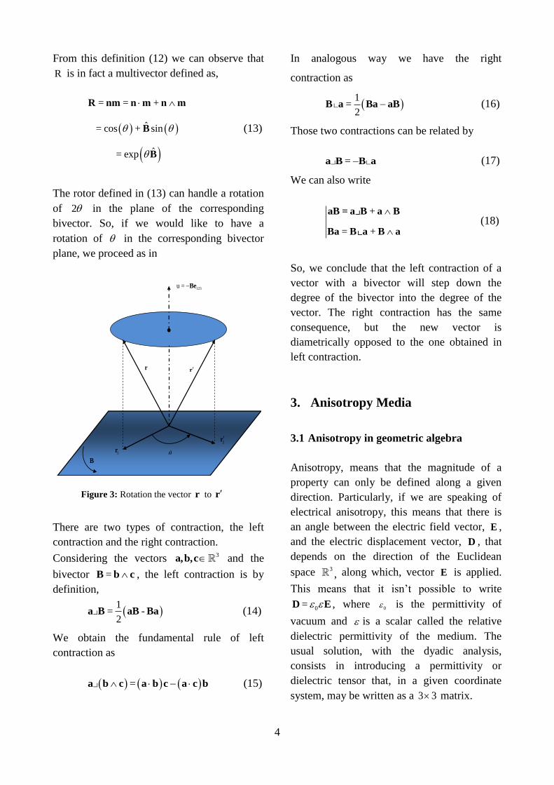
Figure 3: Rotation the vector r to r

5
With geometric algebra 3 , we simply write
0= D E (19)
where E is a dielectric linear function
3 3 ε: that maps vectors to vectors and it
characterizes the medium only along a certain
direction.
Henceforth, it will be considered that the
media in study are not magnetic, lossless,
unbounded and linear. In non magnetic media
we have = 0M , so the relationship between B
and H is same of vacuum, i.e.,
0= B H (20)
Formally, considering figure 4, when an
electric field =E E s
in the direction
characterized by unit vector s is applied, the
media responds with an electric displacement
field =D D t . The relation between s and t is
such that = coss t and = sins t F . Now,
we are in conditions of characterizing the
media correctly. So it follows, in such way:
= = cos
= = sin
ˆ = =sin
ˆ= = = sin
D s D D
D r D D
s tF sr
F E D E D s t F
(21)
s
s
= s = s = s cos
D =
D
E
(22)
The following considerations can also be made
in accordance to Figure 4,
=
= + = = +
ˆ= cos + sin
ˆ= exp
E D
ED E D E D st s t s t
F
ED F
(23)
(1.2)
In expression (22), s = s is the
permittivity along s and s is the dielectric
function. Specifically, in an anisotropic
medium, to each direction s of the space
corresponds a scalar s = s s .
In order to exemplify better this concept of
relative dielectric constant let us consider an
example. Admitting that the linear operator 3 3ε : has three real distinct eigenvalues
1 2 3> > . For convenience of future
calculus, consider the following:
2
3 3 3 1
2 2 2
3 1 2 1 2 1
2 2
1 1 3 2 3
= + 2 = 2
+ =1 = = 2
= 2 = 2
(24)
Figure 4: Electrical anisotropy characterized by bivector
= F E D .
6
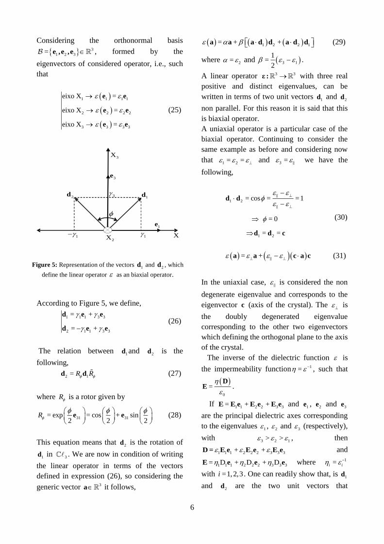
Considering the orthonormal basis
3
1 2 3= e ,e ,e , formed by the
eigenvectors of considered operator, i.e., such
that
1 1 1 1
2 2 2 2
3 3 3 3
eixo X =
eixo X =
eixo X =
e e
e e
e e
(25)
.
According to Figure 5, we define,
1 1 1 3 3
2 1 1 3 3
= +
= +
d e e
d e e (26)
The relation between 1d and
2d is the
following,
2 1= R R d d (27)
where R is a rotor given by
31 31= exp = cos + sin2 2 2
R
e e (28)
This equation means that 2d is the rotation of
1d in 3 . We are now in condition of writing
the linear operator in terms of the vectors
defined in expression (26), so considering the
generic vector 3a it follows,
1 2 2 1= + + a a a d d a d d (29)
where 2= and 3 1
1=
2 .
A linear operator 3 3ε : with three real
positive and distinct eigenvalues, can be
written in terms of two unit vectors 1d and
2d
non parallel. For this reason it is said that this
is biaxial operator.
A uniaxial operator is a particular case of the
biaxial operator. Continuing to consider the
same example as before and considering now
that 1 2= =
and 3 = we have the
following,
1 2
1 2
= cos = = 1
= 0
= =
d d
d d c
(30)
= + a a c a c (31)
In the uniaxial case, is considered the non
degenerate eigenvalue and corresponds to the
eigenvector c (axis of the crystal). The is
the doubly degenerated eigenvalue
corresponding to the other two eigenvectors
which defining the orthogonal plane to the axis
of the crystal.
The inverse of the dielectric function is
the impermeability function 1= , such that
0
=
DE .
If 1 1 2 2 3 3= + +E E e E e E e and
1e , 2e and
3e
are the principal dielectric axes corresponding
to the eigenvalues 1 , 2 and
3 (respectively),
with 3 2 1> > , then
1 1 1 2 2 2 3 3 3+ + D = E e E e E e and
1 1 1 2 2 2 3 3 3= D + D + D E e e e where 1=i i
with =1,2,3i . One can readily show that, is 1d
and 2d are the two unit vectors that
2d
3e
3X
1d
1
1e
1
1X
2X
3
Figure 5: Representation of the vectors 1d and
2d , which
define the linear operator as an biaxial operator.
7
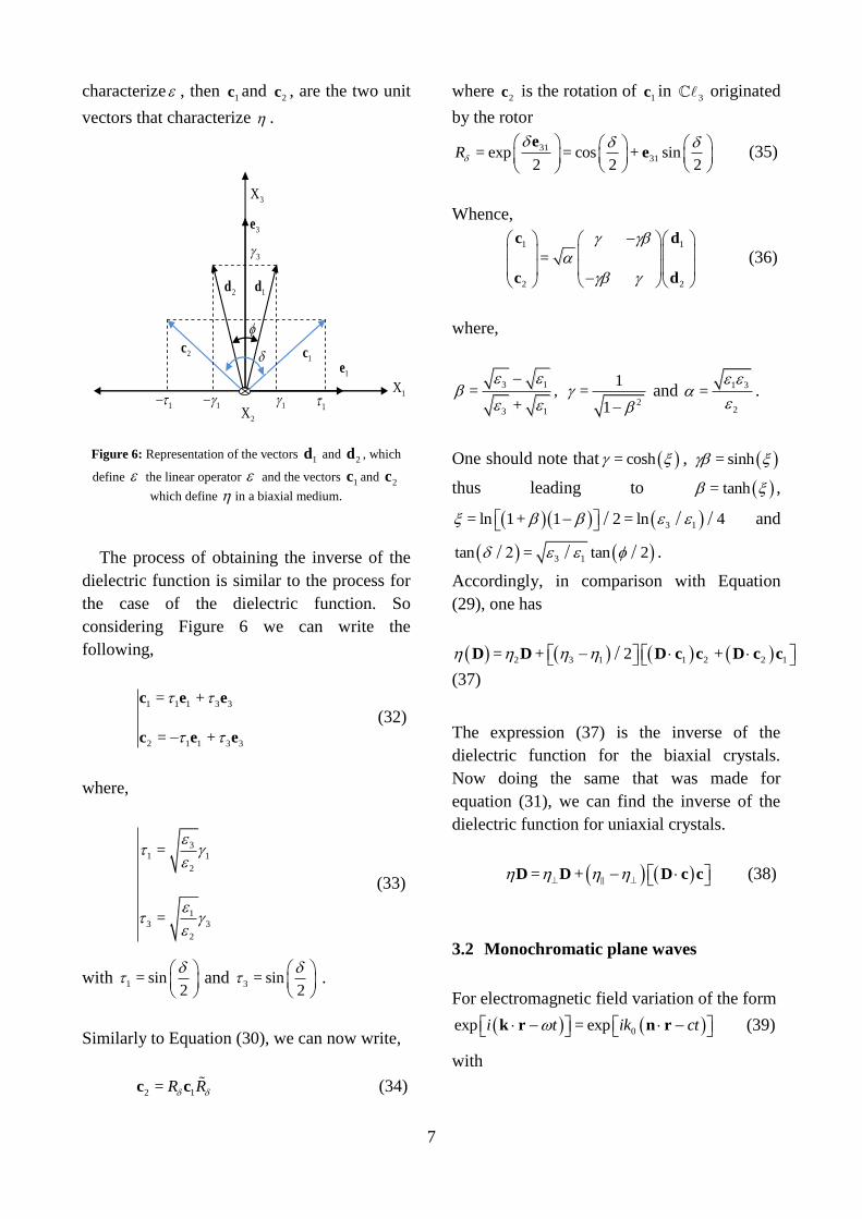
characterize , then 1c and
2c , are the two unit
vectors that characterize .
The process of obtaining the inverse of the
dielectric function is similar to the process for
the case of the dielectric function. So
considering Figure 6 we can write the
following,
1 1 1 3 3
2 1 1 3 3
= +
= +
c e e
c e e
(32)
where,
3
1 1
2
1
3 3
2
=
=
(33)
with 1 = sin2
and 3 = sin2
.
Similarly to Equation (30), we can now write,
2 1= R R c c (34)
where 2c is the rotation of
1c in 3 originated
by the rotor
31
31= exp = cos + sin2 2 2
R
ee (35)
Whence,
1 1
2 2
=
c d
c d
(36)
where,
3 1
3 1
= , +
2
1=
1
and
1 3
2
=
.
One should note that = cosh , = sinh
thus leading to = tanh ,
3 1= ln 1+ 1 2 = ln 4 ∕ ∕ ∕ and
3 1tan = tan 2 ∕ ∕ ∕ .
Accordingly, in comparison with Equation
(29), one has
2 3 1 1 2 2 1= + 2 + D D D c c D c c∕
(37)
The expression (37) is the inverse of the
dielectric function for the biaxial crystals.
Now doing the same that was made for
equation (31), we can find the inverse of the
dielectric function for uniaxial crystals.
= + D D D c c (38)
3.2 Monochromatic plane waves
For electromagnetic field variation of the form
0exp = expi t ik ct k r n r (39)
with
1
1
2X
1 1
1e
1X
2c
2d
1d
1c
3X
3
3e
Figure 6: Representation of the vectors 1d and
2d , which
define the linear operator and the vectors 1c and
2c
which define in a biaxial medium.

8
0 0= =
ˆ=
k kc
n
k n
n k
(40)
Maxwell equation in 3 may be simply
written, for source-free regions, as
123
123
=
=
= 0
= 0
c
c
n E Be
n H De
n D
n H
(41)
3.3 Uniaxial crystals
As we saw previously, for the case of a
uniaxial medium we have the following
dielectric function:
= + E E c E c (42)
Normally, an uniaxial crystals it is common to
consider 2= no and 2= ne . The crystals are
considered positive when > and negative
if < .
Remembering the constitutive relations of the
media in equation (19) and also remembering
that the media is non magnetic, 0= B H , the
following comes,
2 2
123 123 0 123
0
= =
=
1 = =
n n n
cc
n n E E E n E
n Be n B e = n H e
D E
(43)
Analyzing the expression (43), we can infer
the following,
2 2
2
= =
= =
n n
n
E E E E
E E E E E E
(44)
The parallel component of electric field, E , is
defined as its component as k̂ , i.e., such that
ˆ = 0k E .
2
2 2 2
1 1= =
= =
n n
n n n
E n E E n E n
E E E E n E n
(45)
Considering the wave equation,
2
ˆ = 0
ˆ ˆ ˆ= = 0n
k E
k E k E k E
(46)
Figure 7: Positive uniaxial crystal
Figure 8: Negative uniaxial crystal

9
One should note that,
0 2
0
0 2 2
0 0
0 0
1= =
1 1
= +
ˆ ˆ= +
e o
n
= =n n
E E c E c
k E k E c E k c
(47)
Finally we get the wave equation in a uniaxial
crystal.
2 2
0 0ˆ ˆ1 + = 0 n n k E c E k c (48)
Applying the left contraction with ˆ k c to
equation (48) we obtain the two eigenwaves or
isonormal wave (extraordinary wave and
ordinary wave) of the uniaxial crystal
2
2 2
0 0
onda ordináriaonda extraordinária
ˆ1 + = 0n n
k c c E
(49)
Finally we can obtain from (49) the equation
of the ordinary wave,
2 2
0
0
1= =n n
(50)
And the equation of the extraordinary wave,
2 2
2
2 22 2ˆ ˆ
o e
e o
n nn =
n n k c k c
(51)
4.2 Biaxial crystals
Considering the equations (29), (37), (40), (41)
and monochromatic plane wave propagation in
a biaxial media, it comes immediately, like we
saw for a uniaxial crystal,
2
ˆ ˆ=
n
E = E
E E E = E E k k
(52)
Accordingly, in terms of permeability function
of equation (39) we may also write
2
ˆ = 0
= n
k w
w E E
(53)
Using a similar procedure to that used for the
case of uniaxial crystals the wave equation for
the biaxial crystals, i.e.,
2
0
2
0 1 2 2 1
ˆ1 +
ˆ ˆ+
n
n
k E
c E k c c E k c (54)
Where 0 2= and 3 1
0 =2
.
Introducing the following vectors,
1 123
2 123
ˆ=
ˆ=
u k c e
v k c e (55)
and applying the left contraction of bivectors
1ˆ k c and 2
ˆ k c with (38), with equation (54),
we obtain,
2 2
0
1 22
0 0
2 2
0
2 12
0 0
=1 +
=1 +
n
n
n
n
uc E c E
u v
vc E c E
u v
(56)
The eingenwaves corresponding to the
direction of propagation k̂ (the normal wave)
are characterized by two distinct refractive
indexes (birefringence), such that n and n
,
such that
2 2
0 02
1= +
n
u v u v (57)

10
Analyzing the equation (57), we can conclude
that for waves propagating along 1c or
2c we
have, according to equation (54), = 0 u or
= 0v (respectively) and hence 2
2
0
1= =n
,
i.e., the two refractive indexes are equal. But
then, according to the definition of optic axes,
we conclude that the two unit vectors 1c and
2c
that characterize the impermeability function
are, in fact, the two optic axes of the biaxial
crystal. These two waves, contrarily to what
happens for uniaxial crystals, cannot be
divided into ordinary and extraordinary waves,
because both of them have simultaneously
characteristics of both ordinary and
extraordinary waves as we can see in Figure 6.
4. Retarder plates
A retarder (or waveplate) alters the
polarization of light in a manner on the
retardance and the angle between the retarder
fast axis and the input plane of polarization.
The most common types of waveplates are
quarter-wave plates (λ/4 plates) and half-wave
plates (λ/2 plates), where the difference of
phase delays between the two linear
polarization directions is π/2 or π, respectively,
corresponding to propagation phase shifts over
a distance of λ / 4 or λ / 2, respectively.
4.1 Quarter-Wave retarder
A quarter-wave retarder is used to convert
linear polarization to circular polarization and
vice-versa. It change linearity polarized light
to circularly polarized light, when the angle
between the input polarization and the retarde
fast axis is 45 . The thickness of the quarter
waveplate is such that the phase difference is
4 1 4, Zero order , or certain multiple of
1 4 -wavelength 2 1 1 4, multiple orderm .
A quarter wave retarder has 90 .
4.2 Half -Wave retarder
When the angle between the retarder fast axis
and the input plane of polarization is 45°,
horizontal polarized light is converted to
vertical. A half-wave retarder rotates a linear
polarized input by twice the angle between the
retarder fast axis and the input plane of
polarization, as shown in figure 7. The
thickness of half waveplate is such that the
phase difference is 2 1 2, Zero order or
3X
1X
2c 1c
1
1
3
2
3
2
+n
n
1
2
Figure 9: Representation of the refractive indexes, which
correspond to the eigenwaves of the biaxial crystal
Figure 10: Conversion between linear and circular polarization
by a quarter-wave plate.

11
certain multiple of 1 2 -wavelength
2 1 1 2, multiple orderm . A half wave
retarder has 180 of retardance.
4.3 Multiple-order and Zero-order plates
The retarder plates may by zero-order i.e.,
m = 0 or multiple order, with m 1 .
The zero-order retarders are almost impossible
to fabricate because the have extremely small
thicknesses, but may be constructed from two
multiple-order retarders with handlable
thicknesses. Regarding multiple order plates
are easy to fabricate but have a disadvantage
of having reduced sensitivity to small
deviations.
4.2 Conclusions and future work
In this thesis were studied the fundamentals of
basic algebra geometry of Euclidean space.
Layed up and studied the product which
characterizes this algebra, the product
geometric or Clifford. This product is the sum
of the inner product with the outer product,
and is generally not commutative and
associative however is invertible. Regarding
the outer product (Grassmann been found that
this is definable in n dimensions and is
independently any metric, unlike the cross
product Gibbs which is definable in three
dimensions and only requires a metric.
Through outer product appears new geometric
objects, the bivector (segment oriented plan)
result of exterior product of two vectors, and
trivector (volume oriented) outcome of
exterior product of three vectors. Stands out
even of extreme importance two operators
such as the rotors which allow the making of
spatial rotations and planar rotations and
contractions of vectors are useful to define the
geometric product of vectors for bivectores
and vice versa. The geometric algebra of
Euclidean space allows complete formulation
of the developments of the classical areas of
physics, mainly from electromagnetism.
In the context of electromagnetism, geometric
algebra stand out showed up tensor algebra for
its independence of any coordinate system,
where the concept of tensor is unnecessary.
With geometric algebra the study of the
propagation of electromagnetic waves in a
uniaxial and biaxial crystal can the simplified,
without resorting the properties of matrices, as
once was done using tensor calculus or dyadic.
It becomes possible to determine the refractive
indices for any direction of the optical axis,
and any direction of propagation. This paper
aims to disclose geometric algebra as a clear
structure, intuitive and geometric as well as
becoming an universal and unifying language
for the study and application in different areas
of physics and engineering, in this case, as an
application to anisotropic media. As an
application in anisotropic media retardant half-
wave plates, quarter-wave and full-wave are
analyses.
.
References
[1] C. Doran and A. Lasenby, Geometric Algebra for
Physicists (Cambridge, UK: Cambridge University Press,
2003)
[2] D. Hestenes, New Foundation for Classical Mechanics
(Dordrecht, The Netherlands: kluwer Academic Publishers,
2nd ed., 1999)
[3]http://specialoptics.com/pdf/wp_retardation_plate_theory.p
df , 03-06-12
Figure 11: Rotation of linear polarization by a half-wave
plate.

12
[4] http://www.yorku.ca/marko/PHYS2212/Lab8.pdf,
03-06-12
[5] L. Dorst, D. Fontijne, and S. Mann, Geometric Algebra for
Computer Science (Amsterdam: Morgan Kaufmann
Publishers, Elsevier, 2007)
[6] P Lounesto, Clifford Algebra and Spinors (Cambridge,
UK: Cambridge University Press, 2nd ed., 2002)
[7] C.R. Paiva, “ Álgebra Geométrica do Espaço: Introdução”.
Departamento de Engenharia Electrotécnica e de
Computadores, Instituto Superior Técnico, 2008.
[8] C.R. Paiva, “ Aspectos Geométricos do
Electromagnetismo”. Departamento de Engenharia
Electrotécnica e de Computadores, Instituto Superior Técnico,
2008.
[9] C.R. Paiva, “Álgebra Geométrica do Espaço: Aplicações”.
Departamento de Engenharia Electrotécnica e de
Computadores, Instituto Superior Técnico, 2008/2009.
[10] C.R. Paiva, “Meios Anisotrópicos”. Departamento de
Engenharia Electrotécnica e de Computadores, Instituto
Superior Técnico, 2002/2003.
[11] S.A. Matos, M.A. Ribeiro and C.R. Paiva, “Anisotropy
without tensors: a novel approach using geometric álgebra”
Optics Express, Vol. 15, No. 23, pp.15175-15186, November
2007.
[12] C. R. Paiva, “Meios Anisotrópicos”. Departamento de
Engenharia Electrotécnica e de Computadores, Instituto
Superior Técnico, 2008/2009.
[13] S. A. Matos, C. R. Paiva, and A. M. Barbosa,
“Anisotropy done right: a geometric algebra approach,” Eur.
Phys. J. Appl. Phys. 49, 33006 (2010).
[14] D. Hestenes, “Oersted Medal Lecture 2002: Reforming
the mathematical language of physics,” American Journal of
Physics, Vol. 71, No. 2, pp. 104-121, February 2003.
[15] H. C. Chen, Theory of Electromagnetic Waves: A
Coordinate-Free Approach. New York: McGraw-Hill, 1985.
[16] J. A. B. Faria, Óptica Fundamentos e Aplicações, pp.
159-163. Lisboa: Editorial Presença, 1994.
[17] A. Yariv, Optical Electronics in Modern
Communications, pp. 17-27. New York: Oxford University
Press, 1997.


![[Howard a.] Álgebra Lineal](https://img.pdfslide.us/doc/110x75/563dbb1d550346aa9aaa6489/howard-a-algebra-lineal.jpg)