Embed Size (px)
Citation preview
ORIGINAL RESEARCH
Analytical investigation of pile–soil interaction in sand underaxial and lateral loads
Ahmed Abdel-Mohti • Yasser Khodair
Received: 3 September 2013 / Accepted: 17 March 2014 / Published online: 17 April 2014
� The Author(s) 2014. This article is published with open access at Springerlink.com
Abstract This paper presents a numerical study of pile–
soil interaction due to application of axial and lateral loads
to piles in sand. The pile–soil interaction was analyzed
using the finite difference (FD) software LPILE and two
finite element (FE) software. The three-dimensional (3D)
FE models of pile–soil interaction have been created using
Abaqus/Cae and SAP2000. Various types of soft soil were
studied, such as loose, medium, and dense sand. A lateral
displacement of 2 cm was applied to the top of the pile
while maintaining a zero slope in a guided fixation. A
combined lateral and axial load of 300 kN was also stud-
ied. The paper compared between the bending moments
and lateral displacements along the depth of the pile
obtained from the FD solutions and FE analyses. A para-
metric study was conducted to study the effect of crucial
design parameters such as the modulus of elasticity of soil
and the number of nonlinear soil springs that can be used to
model the soil. A good agreement between the results
obtained by the FE models and the FD solution was
observed. Also, the FE models were capable of predicting
the pile–soil interaction for all types of soft soil.
Keywords Pile � Pile-soil interaction � Pile loads
Introduction
The pile foundation is used when it is necessary to transfer
the loads from the superstructure and abutment to a
stronger soil beneath the weak soil near the ground surface,
which is not capable of carrying the loads. The pile foun-
dations are subjected to vertical loads as well as lateral
loads. To design piles, it is desired to understand pile–soil
interaction. Moreover, it is important to construct flexible
abutments with piles to permit longitudinal movement in
bridges due to thermal, shrinkage, and creep effects
(Dicleli and Albhaisi 2003). The steel H-pile (HP-sections)
is the most common type of piles that are used to support
the abutment of integral bridges.
The pile–soil interaction is a complex problem. The
soil is not isotropic, homogeneous, or linear therefore it is
important to account for these complicated characteristics
(Dutta and Roy 2001). The interaction between the
structure and soil has a potential to affect the behavior of
the structure (Abdel-Mohti and Pekcan 2013a, b). It is
important to evaluate this pile–soil interaction under the
effect of both axial and lateral loads. A number of
approaches can be used to analyze piles subjected to a
lateral loading such as subgrade reaction approach, elastic
approach, and finite element approach. Most engineers
prefer the p–y curve method over elastic continuum and
finite element analysis methods. In each approach, it may
be possible to conduct static or dynamic analysis and also
the behavior of pile, soil, or pile–soil interaction may be
linear or nonlinear. The p–y approach, Winkler subgrade,
models the lateral soil–pile interaction using a set of
empirical p–y curves (Hartog 1952). In the subgrade
modulus reaction approach (Reese and Matlock 1956;
Georgiadis and Butterfield 1982; Sawant et al. 1996), the
pile is modeled as an elastic beam while the continuum of
A. Abdel-Mohti
Civil Engineering Department, Ohio Northern University,
525 South Main St., Ada, OH 45810, USA
e-mail: [email protected]
Y. Khodair (&)
Department of Civil Engineering and Construction, Bradley
University, 1501 West Bradley Avenue, Peoria, IL 61625, USA
e-mail: [email protected]
123
Int J Adv Struct Eng (2014) 6:54
DOI 10.1007/s40091-014-0054-5
the soil is ignored as the soil is modeled using a series of
independent springs having constant stiffness. In spite of
the simplicity of this method, it can provide reasonably
accurate results. Other approaches include the elastic
continuum approach (Spillers and Stoll 1964; Poulos
1971; Banerjee and Davies 1978) and the finite element
method. In the elastic approach, the soil is assumed as an
elastic continuum. Recently, numerical methods have
gained momentum; therefore, a number of researchers
used linear and nonlinear finite element analysis to study
the pile–soil interaction (Yegian and Wright 1973; Desai
1974; Desai and Abel 1974; Desai and Appel 1976; Ku-
hlemeyer 1979; Desai et al. 1981; Zaman et al. 1993;
Narsimha Rao and Ramkrishna 1996; Bransby and
Springman 1999; Ng and Zhang 2001; Sawant and De-
waikar 2001; Krishnamoorthy and Anil 2003; Krishna-
moorthy and Nitin 2005; Dewaikar et al. 2007; Zhang
2009; Chore et al. 2010; Muqtadir and Desai 1986;
Pressley and Poulos 1986; Brown and Shie 1990a, b,
1991; Trochanis et al. 1991; Kimura et al. 1995; Wakai
et al. 1999; Pan et al. 2002). The finite element approach
has a capability to deal with any configurations of struc-
tures and soil. It was concluded that finite element ana-
lysis can be a reliable tool to predict the pile–soil
interaction under the effect of lateral load since it can
account for the soil mass and the nonlinear nature of pile–
soil interaction. It is recommended to orientate the pile for
bending about the major axis to improve the displacement
capacity of the bridge under low-cycle fatigue while it is
recommended to change the orientation of the pile for
bending about minor axis if the flexural capacity of the
abutment governs the displacement capacity of the bridge
(Dicleli and Albhaisi 2003).
The effect of various parameters, such as profiles of soil
layers, pile length, and soil layer properties has been
investigated (Avaei et al. 2008; Davisson and Gill 1963;
Lee and Karunaratne 1987; Reese et al. 1981). LPILE
program, developed by Ensoft, uses a method that assumes
Fig. 1 Soil property inputs for
medium sand soil in the finite
difference (FD) LPILE model
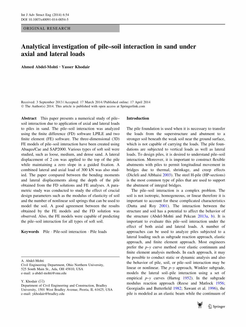
Fig. 2 Master surface in Abaqus/Cae defining the contact behavior
between steel and sand and the rigid body elements at the top of the
pile embedded in the pile cap
54 Page 2 of 16 Int J Adv Struct Eng (2014) 6:54
123
p–y curves (Reese et al. 2004). David and Forth (2011)
investigated the use of finite element models at which the
structure was assumed to behave linearly and soil is non-
linear. Sanjaya Kumar et al. (2007) investigated the per-
formance of laterally loaded piles in high marine clay soil
using ABAQUS and p–y method. Also, Suleiman et al.
(2010) conducted an experiment to measure the pile–soil
interaction in laterally loaded piles having small diameters
in loose sand soil. Chioui and Chenu (2007) presented an
equivalent model for a linear pile–soil interaction of lat-
erally loaded piles using a set of equivalent soil springs.
The soil commonly behaves like an elastic–plastic
material. There are a large number of available soil con-
stitutive models that can be used to represent the soil
including Winkler Model, Mohr–Coulomb Model, (Modi-
fied) Cam–Clay model, Duncan–Chang Model, and Elastic
Continuum Model. The Winkler Model is considered a
simplified model, in which the soil can be modeled using
linear or nonlinear springs. The Mohr–Coulomb Model is
elastic–perfectly plastic and takes into account the effect of
stresses on the strength of soil. The failure criteria are
defined by the friction angles and cohesion of soil. The
(Modified) Cam–Clay Model is an elastic–plastic strain
hardening model at which nonlinearity is modeled using
hardening plasticity. The Duncan–Chang Model is also
called hyperbolic model and it is stress-dependent model
used to describe nonlinearity of cohesive and cohesionless
soil. The Elastic Continuum Model represents infinite soil
medium.
Due to the change in temperature, the bridge experi-
ences expansions and contractions, which in turn are
experienced by the supporting piles. The effect of this daily
and seasonal temperature change is dependent on the
magnitude of temperature change and the length of the
bridge. This thermal loading shall be considered in the
design of piles.
This research examines the pile–soil interaction for
various types of sand soil including loose, medium, and
dense sand. The objectives of this research are to: (1) use a
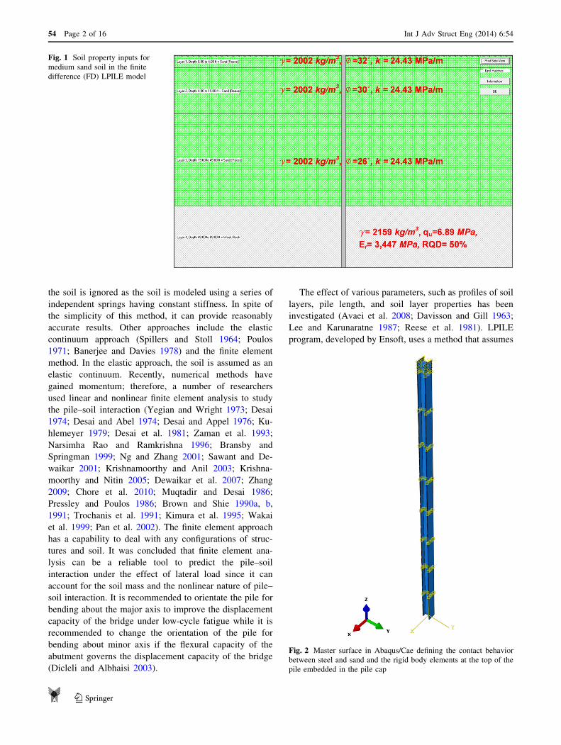
Fig. 3 A schematic diagram of the cross-sectional elevation of the Instrumented Bridge (Khodair and Hassiotis 2013)
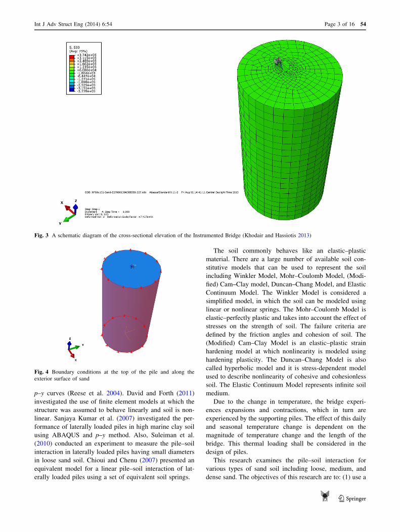
Fig. 4 Boundary conditions at the top of the pile and along the
exterior surface of sand
Int J Adv Struct Eng (2014) 6:54 Page 3 of 16 54
123
number of software to evaluate pile–soil interaction, such
as the finite difference software LPILE (2012) and the
finite element software Abaqus/Cae and SAP2000, (2)
compare the bending moments and lateral displacements
induced along the depth of the pile using the finite differ-
ence method and the finite element models, and (3) conduct
a parametric study to determine the effect of relevant
design parameters which include the soil modulus of
elasticity, varying the sand soil type including loose,
medium, dense sand, and varying the number of soil
springs on the pile induced bending moment and lateral
displacements along its depth. In order to achieve the
objectives of this research, the authors (1) employed a 2D
finite difference (FD) method model using LPILE, (2)
developed 3D finite element (FE) models of the pile–soil
system using Abaqus/Cae and SAP2000, and (3) analyzed
the effect of crucial design parameters, which were listed
before, on piles bending moment and lateral displacement
and then drew our conclusions.
Bridge description
The bridge studied is a steel girder bridge. It consists of one
span with span length of about 45.5 m and width of
32.18 m. The reinforced concrete deck is *25.4 cm thick
and the spacing between stringers is 3.35 m. The abutment
is supported using HP 16 9 101 A572 steel piles.
Finite difference method model
A 2D finite difference (FD) model of the pile–soil inter-
action was developed using LPILE (2012). The model is
based on stress equilibrium in 2D solved using the finite
difference method. The pile was modeled according to the
exact dimensions of an HP 16 9 101. The soil profile
consists of four layers: three layers of sand and one layer of
weak rock (Fig. 1). The angles of friction of the three
layers of sand are 32�, 30�, and 26� from top to bottom.
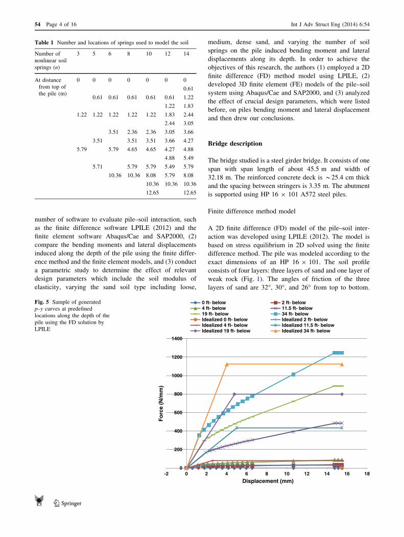
Table 1 Number and locations of springs used to model the soil
Number of
nonlinear soil
springs (n)
3 5 6 8 10 12 14
At distance
from top of
the pile (m)
0 0 0 0 0 0 0
0.61
0.61 0.61 0.61 0.61 0.61 1.22
1.22 1.83
1.22 1.22 1.22 1.22 1.22 1.83 2.44
2.44 3.05
3.51 2.36 2.36 3.05 3.66
3.51 3.51 3.51 3.66 4.27
5.79 5.79 4.65 4.65 4.27 4.88
4.88 5.49
5.71 5.79 5.79 5.49 5.79
10.36 10.36 8.08 5.79 8.08
10.36 10.36 10.36
12.65 12.65
0
200
400
600
800
1000
1200
1400
-2 0 2 4 6 8 10 12 14 16 18
Fo
rce
(N/m
m)
Displacement (mm)
0 ft- below 2 ft- below4 ft- below 11.5 ft- below19 ft- below 34 ft- belowIdealized 0 ft- below Idealized 2 ft- belowIdealized 4 ft- below Idealized 11.5 ft- belowIdealized 19 ft- below Idealized 34 ft- below
Fig. 5 Sample of generated
p–y curves at predefined
locations along the depth of the
pile using the FD solution by
LPILE
54 Page 4 of 16 Int J Adv Struct Eng (2014) 6:54
123
The pile is oriented such that bending is about the weak
axis. Figure 1 shows the properties used to define the sand
layers and weak rock layer in LPILE. Also, in LPILE, the
sand soil type was varied as loose, medium, and dense
having k of 6,790, 24,430, and 61,000 kPa/m, respectively.
Finite element models
Two 3D finite element models of the pile–soil interaction
were developed using the finite element software Abaqus/
Cae and SAP2000 to study the nonlinear behavior of the
soil.
In the Abaqus/Cae model, an elastic model was adopted
for modeling the steel piles with a modulus of elasticity of
200,000 MPa. The studied soils are loose, medium, and
dense sand with c of 2,002 kg/m3 and k varying as 6,790,
24,430, and 61,000 kPa/m, respectively. A strain hardening
model using Mohr–Coulomb failure criterion was adopted
for the soil. For all sands, a Poisson’s ratio of 0.25 and an
angle of internal friction of 30� were used in the definition
of the Mohr–Coulomb failure criterion. To study the loose
sand, the modulus of elasticity of the sand was varied
between 10,000 and 30,000 kPa to determine the proper
modulus of elasticity that can be used to represent the loose
sand. More effort was required to study the medium sand.
The modulus of elasticity of the sand was varied between
10,000 and 69,000 kPa to determine the proper modulus of
elasticity that can be used to represent the medium sand. It
was necessary to further refine the initial values of modulus
of elasticity that were considered to arrive at the proper
modulus of elasticity that can be used to realistically rep-
resent the medium sand. To study the dense sand, larger
values of modulus of elasticity of the sand were considered
and varied between 40,000 and 69,000 kPa to determine
the proper modulus of elasticity that can be used to rep-
resent the dense sand. The interaction between the sand and
the pile was modeled by defining tangential and normal
contact behavior in the FE model. A master and slave
surfaces were defined in the FE model as shown in Fig. 2.
The master surface was represented by the exterior surface
of the pile, and the slave surface by interior surface of the
sand which was extruded according to the exact dimen-
sions of the pile. The tangential contact between the two
surfaces was defined using a friction coefficient of 0.58. A
relatively fine mesh was adopted for the pile and a coarser
mesh was adopted for the sand soil as shown in Fig. 3. In
this model, the pile and sand were modeled using eight-
nodded solid continuum elements (C3D8R) to account for
the continuum nature of the soil in Abaqus/Cae. The bot-
tom of the pile was fixed into the FE model to simulate the
embedment of the pile into rock below a depth of 14.94 m
and the exterior surface of the soil cylinder was fixed to
model the confinement of the soil at its limits as shown in
Fig. 4. The degrees of freedom of the elements at the top of
the pile were restrained to a reference point defined at the
centroid of the pile’s cross section in what defines a rigid
body motion to model the guided fixation occurring due to
the embedment of the top of the pile into the pile cap for a
distance of about 0.3 m.
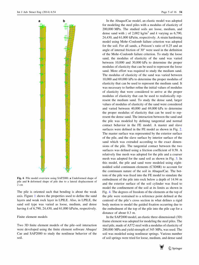
In the SAP2000 model, an elastic three-dimensional (3D)
frame element was adopted for modeling the steel piles. The
steel pile, made of A572 steel with a modulus of elasticity of
200,000 MPa and yield strength of 345 MPa, was used. The
soil was modeled using nonlinear springs. Various number
of soil springs were tried for loose, medium, and dense sand
Fig. 6 Pile model overview using SAP2000. a Undeformed shape of
pile and b deformed shape of pile due to a lateral displacement of
2 cm
Int J Adv Struct Eng (2014) 6:54 Page 5 of 16 54
123

to determine the suitable number and distribution of springs
that can be used with each type of sand. Table 1 shows the
number and distribution of nonlinear soil springs that were
considered and studied for each type of sand. Plastic (Wen)
link element available in SAP2000 was used to model the
hysteresis of soil. The springs were assigned in the longi-
tudinal direction of the bridge. The nonlinear properties of
the link elements were obtained using the generated
p–y curves from the FD solution by LPILE (Fig. 5). The
number of soil springs were varied to investigate the effect
of changing the number of springs on the performance of
the pile and to determine the proper number of springs that
should be used. The seven alternatives (Table 1) include
using 3, 5, 6, 8, 10, 12, and 14 springs along the depth of the
pile: (1) in the 3 springs model, springs were assigned at 0,
1.22, and 5.79 m below the top of the pile, (2) in the 5
springs model, springs were assigned at 0, 0.61, 1.22, 3.51,
and 5.71 m below the top of the pile, (3) in the 6 springs
model, springs were assigned at 0, 0.61, 1.22, 3.51, 5.79,
and 10.36 m below the top of the pile, (4) in the 8 springs
model, springs were assigned at 0, 0.61, 1.22, 2.36, 3.51,
4.65, 5.79, and 10.36 m below the top of the pile, (5) in the
10 springs model, springs were assigned at 0, 0.61, 1.22,
2.36, 3.51, 4.65, 5.79, 8.08, 10.36, and 12.65 m below the
top of the pile, (6) in the 12 springs model, springs were
assigned at 0, 0.61, 1.22, 1.83, 2.44, 3.05, 3.66, 4.27, 4.88,
5.49, 5.79, and 10.36 m below the top of the pile, and (7) in
the 14 springs model, springs were assigned at 0, 0.61, 1.22,
1.83, 2.44, 3.05, 3.66, 4.27, 4.88, 5.49, 5.79, 8.08, 10.36,
and 12.65 m below the top of the pile. The p–y curves were
developed in LPILE at the defined depth locations and
hence the soil stiffness at various depth locations was cal-
culated and hysteretic behavior was obtained. Fixity was
assigned at the bottom of the pile to simulate the embed-
ment of the pile into rock below a depth of 14.94 m as
shown in Fig. 6. The degrees of freedom of the elements at
the top of the pile were restrained in a way to define a rigid
body motion to model the guided fixation due to the
embedment of the top of the pile into the pile cap for a
distance of 30 cm.
Loading
In the first part of the study, a displacement of 2 cm, which
corresponds to a temperature change of 44 �C was applied
to the reference point of the rigid body defined at the top of
the pile to model the lateral displacement caused by
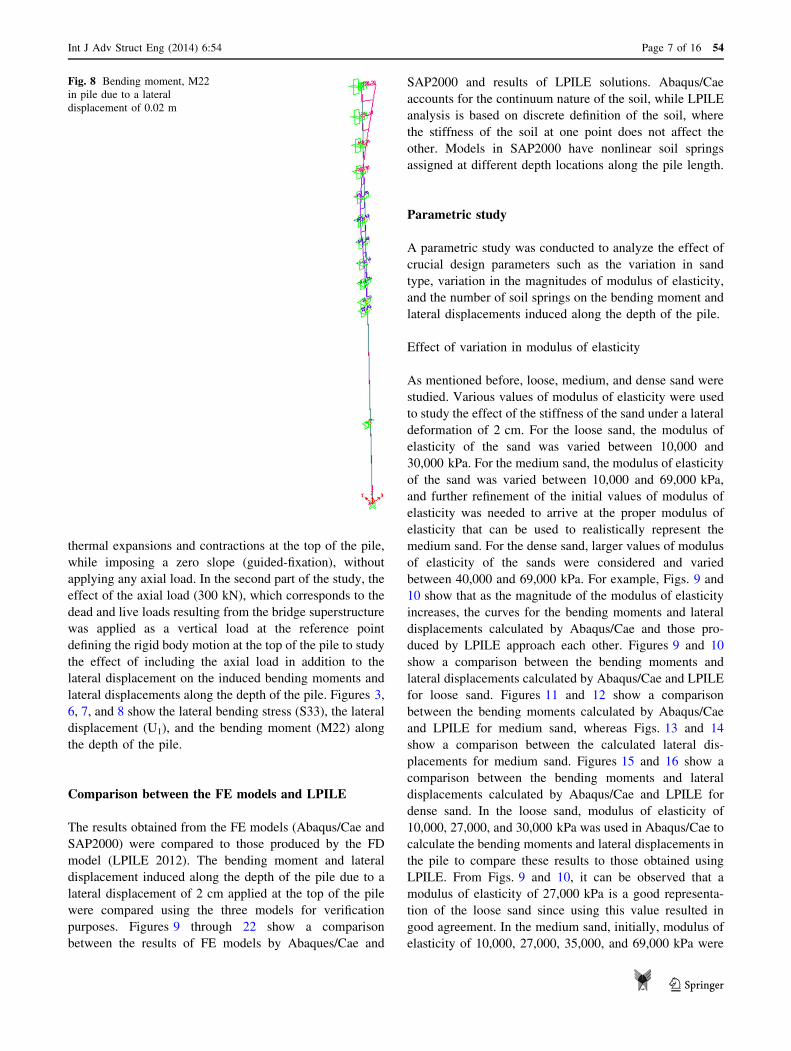
Fig. 7 A contour plot of pile lateral displacement, U1 due to an imposed lateral displacement of 2 cm at the top of the pile
54 Page 6 of 16 Int J Adv Struct Eng (2014) 6:54
123
thermal expansions and contractions at the top of the pile,
while imposing a zero slope (guided-fixation), without
applying any axial load. In the second part of the study, the
effect of the axial load (300 kN), which corresponds to the
dead and live loads resulting from the bridge superstructure
was applied as a vertical load at the reference point
defining the rigid body motion at the top of the pile to study
the effect of including the axial load in addition to the
lateral displacement on the induced bending moments and
lateral displacements along the depth of the pile. Figures 3,
6, 7, and 8 show the lateral bending stress (S33), the lateral
displacement (U1), and the bending moment (M22) along
the depth of the pile.
Comparison between the FE models and LPILE
The results obtained from the FE models (Abaqus/Cae and
SAP2000) were compared to those produced by the FD
model (LPILE 2012). The bending moment and lateral
displacement induced along the depth of the pile due to a
lateral displacement of 2 cm applied at the top of the pile
were compared using the three models for verification
purposes. Figures 9 through 22 show a comparison
between the results of FE models by Abaques/Cae and
SAP2000 and results of LPILE solutions. Abaqus/Cae
accounts for the continuum nature of the soil, while LPILE
analysis is based on discrete definition of the soil, where
the stiffness of the soil at one point does not affect the
other. Models in SAP2000 have nonlinear soil springs
assigned at different depth locations along the pile length.
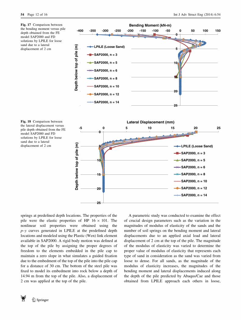
Parametric study
A parametric study was conducted to analyze the effect of
crucial design parameters such as the variation in sand
type, variation in the magnitudes of modulus of elasticity,
and the number of soil springs on the bending moment and
lateral displacements induced along the depth of the pile.
Effect of variation in modulus of elasticity
As mentioned before, loose, medium, and dense sand were
studied. Various values of modulus of elasticity were used
to study the effect of the stiffness of the sand under a lateral
deformation of 2 cm. For the loose sand, the modulus of
elasticity of the sand was varied between 10,000 and
30,000 kPa. For the medium sand, the modulus of elasticity
of the sand was varied between 10,000 and 69,000 kPa,
and further refinement of the initial values of modulus of
elasticity was needed to arrive at the proper modulus of
elasticity that can be used to realistically represent the
medium sand. For the dense sand, larger values of modulus
of elasticity of the sands were considered and varied
between 40,000 and 69,000 kPa. For example, Figs. 9 and
10 show that as the magnitude of the modulus of elasticity
increases, the curves for the bending moments and lateral
displacements calculated by Abaqus/Cae and those pro-
duced by LPILE approach each other. Figures 9 and 10
show a comparison between the bending moments and
lateral displacements calculated by Abaqus/Cae and LPILE
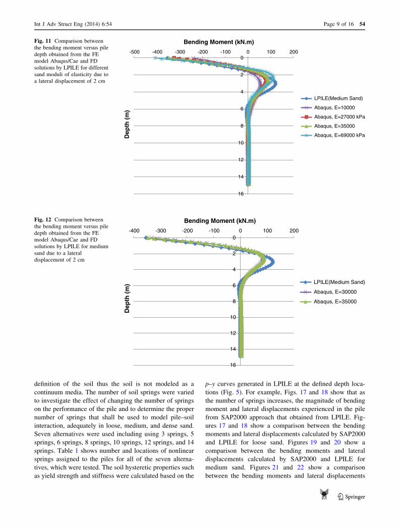
for loose sand. Figures 11 and 12 show a comparison
between the bending moments calculated by Abaqus/Cae
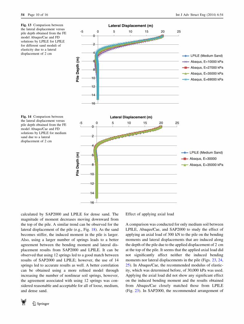
and LPILE for medium sand, whereas Figs. 13 and 14
show a comparison between the calculated lateral dis-
placements for medium sand. Figures 15 and 16 show a
comparison between the bending moments and lateral
displacements calculated by Abaqus/Cae and LPILE for
dense sand. In the loose sand, modulus of elasticity of
10,000, 27,000, and 30,000 kPa was used in Abaqus/Cae to
calculate the bending moments and lateral displacements in
the pile to compare these results to those obtained using
LPILE. From Figs. 9 and 10, it can be observed that a
modulus of elasticity of 27,000 kPa is a good representa-
tion of the loose sand since using this value resulted in
good agreement. In the medium sand, initially, modulus of
elasticity of 10,000, 27,000, 35,000, and 69,000 kPa were
Fig. 8 Bending moment, M22
in pile due to a lateral
displacement of 0.02 m
Int J Adv Struct Eng (2014) 6:54 Page 7 of 16 54
123
used in Abaqus/Cae to calculate the bending moments and
lateral displacements in the pile. Using this set of modulus
of elasticity values did not result in good agreement
between results of Abaqus/Cae and LPILE; therefore, it
was necessary to further refine and hence a modulus of
elasticity of 30,000 kPa was used. It can be observed that a
modulus of elasticity of 30,000–35,000 kPa is a good
representation of the medium sand since using these values
resulted in good agreement as shown in Figs. 11, 12, 13,
and 14. In the dense sand, modulus of elasticity of 40,000,
50,000, and 69,000 kPa were used in Abaqus/Cae to cal-
culate the bending moments and lateral displacements in
the pile and compare these results to those of LPILE as
shown in Figs. 15 and 16. It can be observed that a mod-
ulus of elasticity of 50,000–69,000 kPa is a good
representation of the dense sand since using this value
resulted in good agreement.
It should be noted that soil definition in Abaqus/Cae and
LPILE models was not the same, as explained earlier. In
conclusion, loose, medium, and dense sand can be modeled
using modulus of elasticity of 27,000 kPa, 30,000–35,000
kPa, and 50,000–69,000 kPa, respectively.
Effect of variation in number of soil springs
In SAP2000, various types of sands were also studied
including loose, medium, and dense sand. The soil was
modeled using nonlinear springs that were assigned at
different depths from the top of the pile. This approach is
similar to that in LPILE since it is based on discrete
0
2
4
6
8
10
12
14
16
-400 -300 -200 -100 0 100 200
Dep
th (
m)
Bending Moment (kN.m)
LPILE (Loose Sand)
Abaqus, E=10000
Abaqus, E=27000 kPa
Abaqus, E=30000
Fig. 9 Comparison between the
bending moment versus pile
depth obtained from the FE
model Abaqus/Cae and FD
solutions by LPILE for soft sand
due to a lateral displacement of
2 cm
0
2
4
6
8
10
12
14
16
-5 0 5 10 15 20 25
Pile
Dep
th (
m)
Lateral Displacement (m)
LPILE (Loose Sand)
Abaqus, E=10000 kPa
Abaqus, E=27000 kPa
Abaqus, E=30000
Fig. 10 Comparison between
the lateral displacement versus
pile depth obtained from the FE
model Abaqus/Cae and FD
solutions by LPILE for soft sand
due to a lateral displacement of
2 cm
54 Page 8 of 16 Int J Adv Struct Eng (2014) 6:54
123
definition of the soil thus the soil is not modeled as a
continuum media. The number of soil springs were varied
to investigate the effect of changing the number of springs
on the performance of the pile and to determine the proper
number of springs that shall be used to model pile–soil
interaction, adequately in loose, medium, and dense sand.
Seven alternatives were used including using 3 springs, 5
springs, 6 springs, 8 springs, 10 springs, 12 springs, and 14
springs. Table 1 shows number and locations of nonlinear
springs assigned to the piles for all of the seven alterna-
tives, which were tested. The soil hysteretic properties such
as yield strength and stiffness were calculated based on the
p–y curves generated in LPILE at the defined depth loca-
tions (Fig. 5). For example, Figs. 17 and 18 show that as
the number of springs increases, the magnitude of bending
moment and lateral displacements experienced in the pile
from SAP2000 approach that obtained from LPILE. Fig-
ures 17 and 18 show a comparison between the bending
moments and lateral displacements calculated by SAP2000
and LPILE for loose sand. Figures 19 and 20 show a
comparison between the bending moments and lateral
displacements calculated by SAP2000 and LPILE for
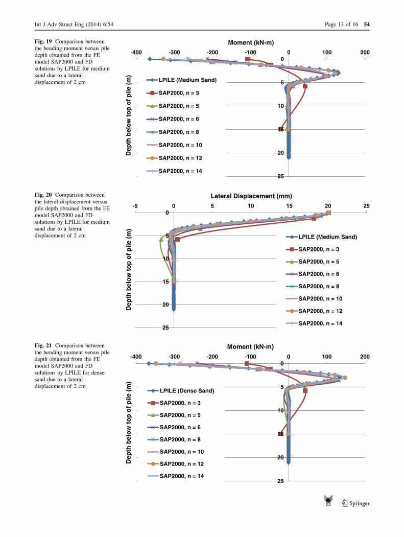
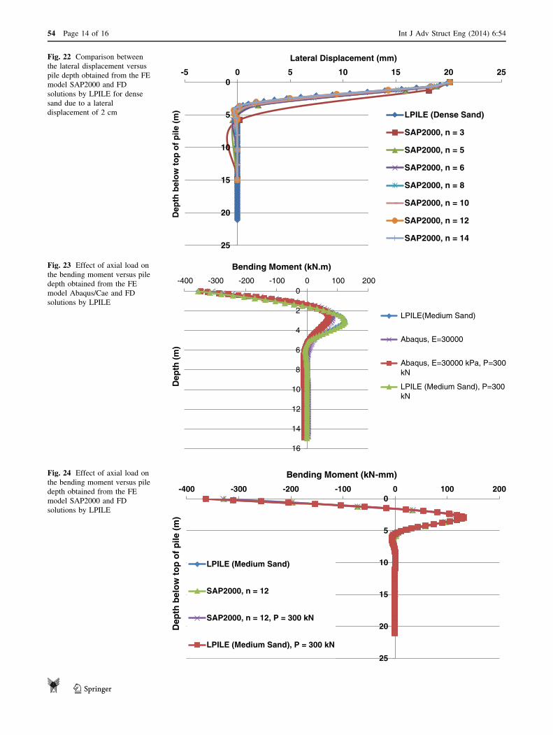
medium sand. Figures 21 and 22 show a comparison
between the bending moments and lateral displacements
0
2
4
6
8
10
12
14
16
-400 -300 -200 -100 0 100 200
Dep
th (
m)
Bending Moment (kN.m)
LPILE(Medium Sand)
Abaqus, E=30000
Abaqus, E=35000
Fig. 12 Comparison between
the bending moment versus pile
depth obtained from the FE
model Abaqus/Cae and FD
solutions by LPILE for medium
sand due to a lateral
displacement of 2 cm
0
2
4
6
8
10
12
14
16
-500 -400 -300 -200 -100 0 100 200
Dep
th (
m)
Bending Moment (kN.m)
LPILE(Medium Sand)
Abaqus, E=10000
Abaqus, E=27000 kPa
Abaqus, E=35000
Abaqus, E=69000 kPa
Fig. 11 Comparison between
the bending moment versus pile
depth obtained from the FE
model Abaqus/Cae and FD
solutions by LPILE for different
sand moduli of elasticity due to
a lateral displacement of 2 cm
Int J Adv Struct Eng (2014) 6:54 Page 9 of 16 54
123
calculated by SAP2000 and LPILE for dense sand. The
magnitude of moment decreases moving downward from
the top of the pile. A similar trend can be observed for the
lateral displacement of the pile (e.g., Fig. 18). As the sand
becomes stiffer, the induced moment in the pile is larger.
Also, using a larger number of springs leads to a better
agreement between the bending moment and lateral dis-
placement results from SAP2000 and LPILE. It can be
observed that using 12 springs led to a good match between
results of SAP2000 and LPILE; however, the use of 14
springs led to accurate results as well. A better correlation
can be obtained using a more refined model through
increasing the number of nonlinear soil springs, however,
the agreement associated with using 12 springs was con-
sidered reasonable and acceptable for all of loose, medium,
and dense sand.
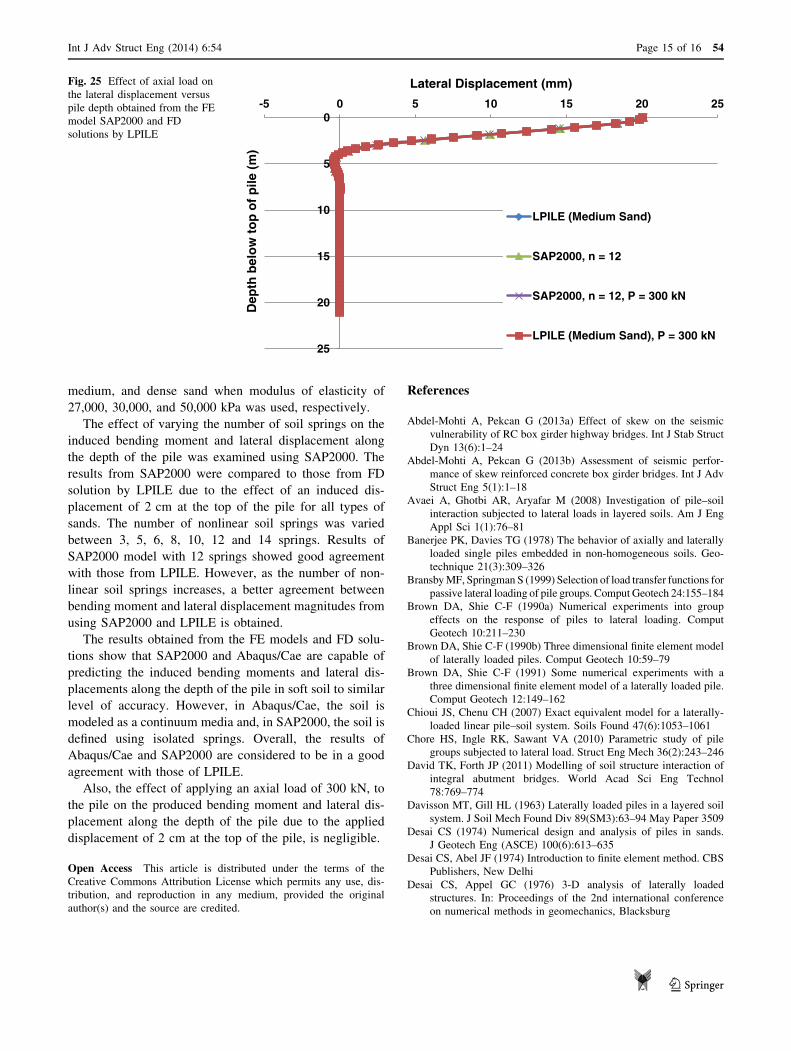
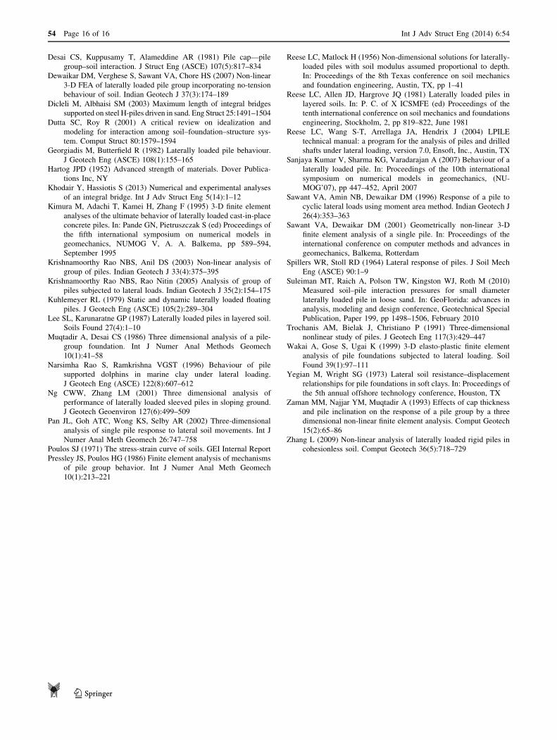
Effect of applying axial load
A comparison was conducted for only medium soil between
LPILE, Abaqus/Cae, and SAP2000 to study the effect of
applying an axial load of 300 kN to the pile on the bending
moments and lateral displacements that are induced along
the depth of the pile due to the applied displacement of 2 cm
at the top of the pile. It seems that the applied axial load did
not significantly affect neither the induced bending
moments nor lateral displacements in the pile (Figs. 23, 24,
25). In Abaqus/Cae, the recommended modulus of elastic-
ity, which was determined before, of 30,000 kPa was used.
Applying the axial load did not show any significant effect
on the induced bending moment and the results obtained
from Abaqus/Cae closely matched those from LPILE
(Fig. 23). In SAP2000, the recommended arrangement of
0
2
4
6
8
10
12
14
16
-5 0 5 10 15 20 25
Pile
Dep
th (
m)
Lateral Displacement (m)
LPILE (Medium Sand)
Abaqus, E=10000 kPa
Abaqus, E=27000 kPa
Abaqus, E=35000 kPa
Abaqus, E=69000 kPa
Fig. 13 Comparison between
the lateral displacement versus
pile depth obtained from the FE
model Abaqus/Cae and FD
solutions by LPILE for LPILE
for different sand moduli of
elasticity due to a lateral
displacement of 2 cm
0
2
4
6
8
10
12
14
16
-5 0 5 10 15 20 25
Pile
Dep
th (
m)
Lateral Displacement (m)
LPILE (Medium Sand)
Abaqus, E=30000
Abaqus, E=35000 kPa
Fig. 14 Comparison between
the lateral displacement versus
pile depth obtained from the FE
model Abaqus/Cae and FD
solutions by LPILE for medium
sand due to a lateral
displacement of 2 cm
54 Page 10 of 16 Int J Adv Struct Eng (2014) 6:54
123
12 springs, which was determined before, was used and it
was found that applying the axial load did not show an
obvious effect on the induced bending moments and lateral
displacements and also these results closely matched those
from LPILE (Figs. 24, 25).
Summary and conclusions
A comparative study to analyze pile–soil interaction in soft
soil under lateral loading was conducted. A 2D finite dif-
ference method model was developed using LPILE (2012).
In this model, the pile was modeled according to the exact
dimensions of a HP 16 9 101. Various types of sands were
studied including loose, medium, and dense sand. The pile
is oriented such that bending is about the weak axis. Two
3D finite element models were developed using the finite
element software Abaqus/Cae and SAP2000. In the 3D
finite element model developed using Abaqus/Cae, both the
pile and the soil were modeled using solid continuum
elements (C3D8R) to account for the continuity of the soil.
An elastic model was adopted for the pile. A Mohr–cou-
lomb failure criterion was defined for the sands. The con-
tact behavior between the piles and the soil was defined
using tangential and normal algorithms in ABAQUS/Cae.
A rigid body motion was defined at the top of the pile by
tying the degrees of freedom of the elements embedded in
the pile cap (30 cm from the top of the pile) to a reference
point at the centroid of the pile’s cross section. In the 3D
finite element model developed using SAP2000, the pile
was modeled using a continuum 3D frame element while
the soil was modeled using a number of nonlinear soil
0
2
4
6
8
10
12
14
16
-500 -400 -300 -200 -100 0 100 200
Dep
th (
m)
Bending Moment (kN.m)
LPILE(Dense Sand)
Abaqus, E=40000 kPa
Abaqus, E=50000 kPa
Abaqus, E=69000 kPa
Fig. 15 Comparison between
the bending moment versus pile
depth obtained from the FE
model Abaqus/Cae and FD
solutions by LPILE for dense
sand due to a lateral
displacement of 2 cm
0
2
4
6
8
10
12
14
16
-5 0 5 10 15 20 25
Pile
Dep
th (
m)
Lateral Displacement (m)
LPILE (Dense Sand)
Abaqus, E=40000
Abaqus, E=50000 kPa
Abaqus, E=69000 kPa
Fig. 16 Comparison between
the lateral displacement versus
pile depth obtained from the FE
model Abaqus/Cae and FD
solutions by LPILE for medium
sand due to a lateral
displacement of 2 cm
Int J Adv Struct Eng (2014) 6:54 Page 11 of 16 54
123
springs at predefined depth locations. The properties of the
pile were the elastic properties of HP 16 9 101. The
nonlinear soil properties were obtained using the
p–y curves generated in LPILE at the predefined depth
locations and modeled using the Plastic (Wen) link element
available in SAP2000. A rigid body motion was defined at
the top of the pile by assigning the proper degrees of
freedom to the elements embedded in the pile cap to
maintain a zero slope in what simulates a guided fixation
due to the embedment of the top of the pile into the pile cap
for a distance of 30 cm. The bottom of the steel pile was
fixed to model its embedment into rock below a depth of
14.94 m from the top of the pile. Also, a displacement of
2 cm was applied at the top of the pile.
A parametric study was conducted to examine the effect
of crucial design parameters such as the variation in the
magnitudes of modulus of elasticity of the sands and the
number of soil springs on the bending moment and lateral
displacements due to an applied axial load and lateral
displacement of 2 cm at the top of the pile. The magnitude
of the modulus of elasticity was varied to determine the
proper value of modulus of elasticity that represents each
type of sand in consideration as the sand was varied from
loose to dense. For all sands, as the magnitude of the
modulus of elasticity increases, the magnitudes of the
bending moment and lateral displacements induced along
the depth of the pile predicted by Abaqus/Cae and those
obtained from LPILE approach each others in loose,
0
5
10
15
20
25
-400 -350 -300 -250 -200 -150 -100 -50 0 50 100 150
Dep
th b
elo
w t
op
of
pile
(m
)
Bending Moment (kN-m)
LPILE (Loose Sand)
SAP2000, n = 3
SAP2000, n = 5
SAP2000, n = 6
SAP2000, n = 8
SAP2000, n = 10
SAP2000, n = 12
SAP2000, n = 14
Fig. 17 Comparison between
the bending moment versus pile
depth obtained from the FE
model SAP2000 and FD
solutions by LPILE for loose
sand due to a lateral
displacement of 2 cm
0
5
10
15
20
25
-5 0 5 10 15 20 25
Dep
th b
elo
w t
op
of
pile
(m
)
Lateral Displacement (mm)
LPILE (Loose Sand)
SAP2000, n = 3
SAP2000, n = 5
SAP2000, n = 6
SAP2000, n = 8
SAP2000, n = 10
SAP2000, n = 12
SAP2000, n = 14
Fig. 18 Comparison between
the lateral displacement versus
pile depth obtained from the FE
model SAP2000 and FD
solutions by LPILE for loose
sand due to a lateral
displacement of 2 cm
54 Page 12 of 16 Int J Adv Struct Eng (2014) 6:54
123
0
5
10
15
20
25
-400 -300 -200 -100 0 100 200
Dep
th b
elo
w t
op
of
pile
(m
)
Moment (kN-m)
LPILE (Medium Sand)
SAP2000, n = 3
SAP2000, n = 5
SAP2000, n = 6
SAP2000, n = 8
SAP2000, n = 10
SAP2000, n = 12
SAP2000, n = 14
Fig. 19 Comparison between
the bending moment versus pile
depth obtained from the FE
model SAP2000 and FD
solutions by LPILE for medium
sand due to a lateral
displacement of 2 cm
0
5
10
15
20
25
-5 0 5 10 15 20 25
Dep
th b
elo
w t
op
of
pile
(m
)
Lateral Displacement (mm)
LPILE (Medium Sand)
SAP2000, n = 3
SAP2000, n = 5
SAP2000, n = 6
SAP2000, n = 8
SAP2000, n = 10
SAP2000, n = 12
SAP2000, n = 14
Fig. 20 Comparison between
the lateral displacement versus
pile depth obtained from the FE
model SAP2000 and FD
solutions by LPILE for medium
sand due to a lateral
displacement of 2 cm
0
5
10
15
20
25
-400 -300 -200 -100 0 100 200
Dep
th b
elo
w t
op
of
pile
(m
)
Moment (kN-m)
LPILE (Dense Sand)
SAP2000, n = 3
SAP2000, n = 5
SAP2000, n = 6
SAP2000, n = 8
SAP2000, n = 10
SAP2000, n = 12
SAP2000, n = 14
Fig. 21 Comparison between
the bending moment versus pile
depth obtained from the FE
model SAP2000 and FD
solutions by LPILE for dense
sand due to a lateral
displacement of 2 cm
Int J Adv Struct Eng (2014) 6:54 Page 13 of 16 54
123
0
5
10
15
20
25
-5 0 5 10 15 20 25
Dep
th b
elo
w t
op
of
pile
(m
)
Lateral Displacement (mm)
LPILE (Dense Sand)
SAP2000, n = 3
SAP2000, n = 5
SAP2000, n = 6
SAP2000, n = 8
SAP2000, n = 10
SAP2000, n = 12
SAP2000, n = 14
Fig. 22 Comparison between
the lateral displacement versus
pile depth obtained from the FE
model SAP2000 and FD
solutions by LPILE for dense
sand due to a lateral
displacement of 2 cm
0
2
4
6
8
10
12
14
16
-400 -300 -200 -100 0 100 200
Dep
th (
m)
Bending Moment (kN.m)
LPILE(Medium Sand)
Abaqus, E=30000
Abaqus, E=30000 kPa, P=300kN
LPILE (Medium Sand), P=300kN
Fig. 23 Effect of axial load on
the bending moment versus pile
depth obtained from the FE
model Abaqus/Cae and FD
solutions by LPILE
0
5
10
15
20
25
-400 -300 -200 -100 0 100 200
Dep
th b
elo
w t
op
of
pile
(m
)
Bending Moment (kN-mm)
LPILE (Medium Sand)
SAP2000, n = 12
SAP2000, n = 12, P = 300 kN
LPILE (Medium Sand), P = 300 kN
Fig. 24 Effect of axial load on
the bending moment versus pile
depth obtained from the FE
model SAP2000 and FD
solutions by LPILE
54 Page 14 of 16 Int J Adv Struct Eng (2014) 6:54
123
medium, and dense sand when modulus of elasticity of
27,000, 30,000, and 50,000 kPa was used, respectively.
The effect of varying the number of soil springs on the
induced bending moment and lateral displacement along
the depth of the pile was examined using SAP2000. The
results from SAP2000 were compared to those from FD
solution by LPILE due to the effect of an induced dis-
placement of 2 cm at the top of the pile for all types of
sands. The number of nonlinear soil springs was varied
between 3, 5, 6, 8, 10, 12 and 14 springs. Results of
SAP2000 model with 12 springs showed good agreement
with those from LPILE. However, as the number of non-
linear soil springs increases, a better agreement between
bending moment and lateral displacement magnitudes from
using SAP2000 and LPILE is obtained.
The results obtained from the FE models and FD solu-
tions show that SAP2000 and Abaqus/Cae are capable of
predicting the induced bending moments and lateral dis-
placements along the depth of the pile in soft soil to similar
level of accuracy. However, in Abaqus/Cae, the soil is
modeled as a continuum media and, in SAP2000, the soil is
defined using isolated springs. Overall, the results of
Abaqus/Cae and SAP2000 are considered to be in a good
agreement with those of LPILE.
Also, the effect of applying an axial load of 300 kN, to
the pile on the produced bending moment and lateral dis-
placement along the depth of the pile due to the applied
displacement of 2 cm at the top of the pile, is negligible.
Open Access This article is distributed under the terms of the
Creative Commons Attribution License which permits any use, dis-
tribution, and reproduction in any medium, provided the original
author(s) and the source are credited.
References
Abdel-Mohti A, Pekcan G (2013a) Effect of skew on the seismic
vulnerability of RC box girder highway bridges. Int J Stab Struct
Dyn 13(6):1–24
Abdel-Mohti A, Pekcan G (2013b) Assessment of seismic perfor-
mance of skew reinforced concrete box girder bridges. Int J Adv
Struct Eng 5(1):1–18
Avaei A, Ghotbi AR, Aryafar M (2008) Investigation of pile–soil
interaction subjected to lateral loads in layered soils. Am J Eng
Appl Sci 1(1):76–81
Banerjee PK, Davies TG (1978) The behavior of axially and laterally
loaded single piles embedded in non-homogeneous soils. Geo-
technique 21(3):309–326
Bransby MF, Springman S (1999) Selection of load transfer functions for
passive lateral loading of pile groups. Comput Geotech 24:155–184
Brown DA, Shie C-F (1990a) Numerical experiments into group
effects on the response of piles to lateral loading. Comput
Geotech 10:211–230
Brown DA, Shie C-F (1990b) Three dimensional finite element model
of laterally loaded piles. Comput Geotech 10:59–79
Brown DA, Shie C-F (1991) Some numerical experiments with a
three dimensional finite element model of a laterally loaded pile.
Comput Geotech 12:149–162
Chioui JS, Chenu CH (2007) Exact equivalent model for a laterally-
loaded linear pile–soil system. Soils Found 47(6):1053–1061
Chore HS, Ingle RK, Sawant VA (2010) Parametric study of pile
groups subjected to lateral load. Struct Eng Mech 36(2):243–246
David TK, Forth JP (2011) Modelling of soil structure interaction of
integral abutment bridges. World Acad Sci Eng Technol
78:769–774
Davisson MT, Gill HL (1963) Laterally loaded piles in a layered soil
system. J Soil Mech Found Div 89(SM3):63–94 May Paper 3509
Desai CS (1974) Numerical design and analysis of piles in sands.
J Geotech Eng (ASCE) 100(6):613–635
Desai CS, Abel JF (1974) Introduction to finite element method. CBS
Publishers, New Delhi
Desai CS, Appel GC (1976) 3-D analysis of laterally loaded
structures. In: Proceedings of the 2nd international conference
on numerical methods in geomechanics, Blacksburg
0
5
10
15
20
25
-5 0 5 10 15 20 25
Dep
th b
elo
w t
op
of
pile
(m
)
Lateral Displacement (mm)
LPILE (Medium Sand)
SAP2000, n = 12
SAP2000, n = 12, P = 300 kN
LPILE (Medium Sand), P = 300 kN
Fig. 25 Effect of axial load on
the lateral displacement versus
pile depth obtained from the FE
model SAP2000 and FD
solutions by LPILE
Int J Adv Struct Eng (2014) 6:54 Page 15 of 16 54
123
Desai CS, Kuppusamy T, Alameddine AR (1981) Pile cap––pile
group–soil interaction. J Struct Eng (ASCE) 107(5):817–834
Dewaikar DM, Verghese S, Sawant VA, Chore HS (2007) Non-linear
3-D FEA of laterally loaded pile group incorporating no-tension
behaviour of soil. Indian Geotech J 37(3):174–189
Dicleli M, Albhaisi SM (2003) Maximum length of integral bridges
supported on steel H-piles driven in sand. Eng Struct 25:1491–1504
Dutta SC, Roy R (2001) A critical review on idealization and
modeling for interaction among soil–foundation–structure sys-
tem. Comput Struct 80:1579–1594
Georgiadis M, Butterfield R (1982) Laterally loaded pile behaviour.
J Geotech Eng (ASCE) 108(1):155–165
Hartog JPD (1952) Advanced strength of materials. Dover Publica-
tions Inc, NY
Khodair Y, Hassiotis S (2013) Numerical and experimental analyses
of an integral bridge. Int J Adv Struct Eng 5(14):1–12
Kimura M, Adachi T, Kamei H, Zhang F (1995) 3-D finite element
analyses of the ultimate behavior of laterally loaded cast-in-place
concrete piles. In: Pande GN, Pietruszczak S (ed) Proceedings of
the fifth international symposium on numerical models in
geomechanics, NUMOG V, A. A. Balkema, pp 589–594,
September 1995
Krishnamoorthy Rao NBS, Anil DS (2003) Non-linear analysis of
group of piles. Indian Geotech J 33(4):375–395
Krishnamoorthy Rao NBS, Rao Nitin (2005) Analysis of group of
piles subjected to lateral loads. Indian Geotech J 35(2):154–175
Kuhlemeyer RL (1979) Static and dynamic laterally loaded floating
piles. J Geotech Eng (ASCE) 105(2):289–304
Lee SL, Karunaratne GP (1987) Laterally loaded piles in layered soil.
Soils Found 27(4):1–10
Muqtadir A, Desai CS (1986) Three dimensional analysis of a pile-
group foundation. Int J Numer Anal Methods Geomech
10(1):41–58
Narsimha Rao S, Ramkrishna VGST (1996) Behaviour of pile
supported dolphins in marine clay under lateral loading.
J Geotech Eng (ASCE) 122(8):607–612
Ng CWW, Zhang LM (2001) Three dimensional analysis of
performance of laterally loaded sleeved piles in sloping ground.
J Geotech Geoenviron 127(6):499–509
Pan JL, Goh ATC, Wong KS, Selby AR (2002) Three-dimensional
analysis of single pile response to lateral soil movements. Int J
Numer Anal Meth Geomech 26:747–758
Poulos SJ (1971) The stress-strain curve of soils. GEI Internal Report
Pressley JS, Poulos HG (1986) Finite element analysis of mechanisms
of pile group behavior. Int J Numer Anal Meth Geomech
10(1):213–221
Reese LC, Matlock H (1956) Non-dimensional solutions for laterally-
loaded piles with soil modulus assumed proportional to depth.
In: Proceedings of the 8th Texas conference on soil mechanics
and foundation engineering, Austin, TX, pp 1–41
Reese LC, Allen JD, Hargrove JQ (1981) Laterally loaded piles in
layered soils. In: P. C. of X ICSMFE (ed) Proceedings of the
tenth international conference on soil mechanics and foundations
engineering, Stockholm, 2, pp 819–822, June 1981
Reese LC, Wang S-T, Arrellaga JA, Hendrix J (2004) LPILE
technical manual: a program for the analysis of piles and drilled
shafts under lateral loading, version 7.0, Ensoft, Inc., Austin, TX
Sanjaya Kumar V, Sharma KG, Varadarajan A (2007) Behaviour of a
laterally loaded pile. In: Proceedings of the 10th international
symposium on numerical models in geomechanics, (NU-
MOG’07), pp 447–452, April 2007
Sawant VA, Amin NB, Dewaikar DM (1996) Response of a pile to
cyclic lateral loads using moment area method. Indian Geotech J
26(4):353–363
Sawant VA, Dewaikar DM (2001) Geometrically non-linear 3-D
finite element analysis of a single pile. In: Proceedings of the
international conference on computer methods and advances in
geomechanics, Balkema, Rotterdam
Spillers WR, Stoll RD (1964) Lateral response of piles. J Soil Mech
Eng (ASCE) 90:1–9
Suleiman MT, Raich A, Polson TW, Kingston WJ, Roth M (2010)
Measured soil–pile interaction pressures for small diameter
laterally loaded pile in loose sand. In: GeoFlorida: advances in
analysis, modeling and design conference, Geotechnical Special
Publication, Paper 199, pp 1498–1506, February 2010
Trochanis AM, Bielak J, Christiano P (1991) Three-dimensional
nonlinear study of piles. J Geotech Eng 117(3):429–447
Wakai A, Gose S, Ugai K (1999) 3-D elasto-plastic finite element
analysis of pile foundations subjected to lateral loading. Soil
Found 39(1):97–111
Yegian M, Wright SG (1973) Lateral soil resistance–displacement
relationships for pile foundations in soft clays. In: Proceedings of
the 5th annual offshore technology conference, Houston, TX
Zaman MM, Najjar YM, Muqtadir A (1993) Effects of cap thickness
and pile inclination on the response of a pile group by a three
dimensional non-linear finite element analysis. Comput Geotech
15(2):65–86
Zhang L (2009) Non-linear analysis of laterally loaded rigid piles in
cohesionless soil. Comput Geotech 36(5):718–729
54 Page 16 of 16 Int J Adv Struct Eng (2014) 6:54
123