Embed Size (px)
Citation preview
EXPERIMENTAL RESPONSE OF A PILE IN SAND UNDER
STATIC AND CYCLIC LATERAL LOADS
by
Pegah Oghabi
A thesis submitted to the Department of Civil Engineering
In conformity with the requirements for
the degree of Master of Applied Science
Queen’s University
Kingston, Ontario, Canada
(May, 2014)
Copyright © Pegah Oghabi, 2014
ii
Abstract
Piles are engineering structures which are subjected to axial and lateral loading. In this
dissertation, pile load tests were performed on a full-scale fabricated pile to understand
lateral pile responses under static and cyclic loading. The experiments were performed on
a fabricated test pile at the Geo-Engineering Laboratory at Queen's University. Dry loose
Olimag Synthetic Olivine sand was used as the test soil.
Instrumentation including axial strain gauges, null sensors (earth pressure sensors) and
string potentiometers were used to monitor pile responses throughout the tests. What
differentiates the current study from previous investigations is direct measurements of
lateral earth pressure on a test pile using those null sensors with conventional
measurements of curvature and deformation. The null sensors of Talesnick (2005) have
‘infinite stiffness’ and calibration that is almost independent of the soil type, soil
condition and stress history, qualities that make the sensor superior to other commercially
available sensors.
The initial pile response under static loading was examined. Previous laterally loaded pile
test programs have utilized curvature measurements to infer moments, and differentiation
of moments to determine lateral forces. Comparisons with the directly measured
pressures confirmed the effectiveness of differentiated moments. To understand offshore
structures, the behaviour of a pile subjected to cyclic loading is examined and explained
by elastic soil response at low load levels and the progressive development of inelastic
response at higher load levels. In addition, the loading condition (i.e. two-way versus
iii
one-way loading) was found to have a substantial effect on pile responses. The pressure
distributions for two-way cyclic loading suggest that the lateral pressure is proportional to
displacement with peak pressures near the ground surface during elastic responses. The
peak lateral pressures move deeper towards the point of rotation with increasing cyclic
loads to generate inelastic responses. However, the lateral pressure response is
consistently inelastic for one-way loading.

iv
Acknowledgements
First, I would like to express my very special thanks to my supervisor, Dr. Ian D. Moore
for giving me an opportunity to pursue this unique research work and for the guidance
and invaluable feedback throughout the duration of this dissertation. The privilege of
study under his supervision will always remain a memorable part of my education.
I would also like to thank Graeme Boyd, Nicholas Andreae and Mark Talesnick for their
technical assistance regarding the instrumentation and implementation of the experiments
in the Geo-Engineering Laboratory. I am also thankful to my colleague, Bryan Simpson,
for always being willing to provide help whenever it was needed.
Special thanks go to Omid Hejazi for his endless support throughout the stressful times of
this study and I reserve this last acknowledgement for my parents whose encouragement,
love and support served as the foundation for all of my past achievements and future
endeavors in life.
v
Table of Contents
Abstract ............................................................................................................................................ ii
Acknowledgements ......................................................................................................................... iv
List of Figures ............................................................................................................................... viii
List of Tables .................................................................................................................................. xi
List of Abbreviations ..................................................................................................................... xii
Chapter 1 INTRODUCTION ........................................................................................................... 1
1.1 GENERAL ............................................................................................................................. 1
1.2 OBJECTIVES ........................................................................................................................ 2
1.3 OUTLINE OF THE DISSERTATION .................................................................................. 3
1.4 REFERENCES ...................................................................................................................... 5
Chapter 2 TEST PILE GEOMETRY, INSTRUMENTATION AND BENDING TEST RESULTS
......................................................................................................................................................... 6
2.1 INTRODUCTION ................................................................................................................. 6
2.2 TEST PILE GEOMETRY AND INSTRUMENTATION ..................................................... 6
2.3 BEAM TEST ......................................................................................................................... 9
2.3.1 Test Setup........................................................................................................................ 9
2.3.2 Loading Procedure ........................................................................................................ 10
2.4 TEST RESULTS .................................................................................................................. 11
2.4.1 Pressure Distribution Response .................................................................................... 11
2.4.2 Deflection-Time Response ............................................................................................ 12
2.4.3 Load-Deflection Response ............................................................................................ 12
2.4.4 Flexural Rigidity ........................................................................................................... 13
2.4.5 Bending Moment Distribution ...................................................................................... 15
2.5 SUMMARY ......................................................................................................................... 17
2.6 REFERENCES .................................................................................................................... 18
Chapter 3 THEORETICAL PREDICTIONS OF AXIAL AND LATERAL LOAD CAPACITIES
....................................................................................................................................................... 34
3.1 INTRODUCTION ............................................................................................................... 34
3.2 AXIAL CAPACITY ............................................................................................................ 35
3.2.1 End Bearing Resistance, Qp .......................................................................................... 36
3.2.2 Shaft Resistance, Qs ...................................................................................................... 38
3.2.3 Ultimate Bearing Capacity, Qu ...................................................................................... 39
vi
3.3 LATERAL CAPACITY ...................................................................................................... 39
3.3.1 Ultimate Lateral Resistance .......................................................................................... 39
3.4 SUMMARY ......................................................................................................................... 42
3.5 REFERENCES .................................................................................................................... 42
Chapter 4 STATIC PILE LOAD TESTS ....................................................................................... 53
4.1 INTRODUCTION ............................................................................................................... 53
4.2 TEST SETUP ....................................................................................................................... 54
4.2.1 Site and Material Description ....................................................................................... 54
4.2.2 Test Pile and Instrumentation ....................................................................................... 55
4.2.3 Limitation for Test Layout ............................................................................................ 58
4.2.4 Test Layout and Loading Procedure ............................................................................. 61
4.3 AXIAL RESPONSE ............................................................................................................ 63
4.3.1 Axial Force Response ................................................................................................... 64
4.3.2 Moment Response ......................................................................................................... 66
4.3.3 Earth Pressure Response ............................................................................................... 66
4.3.4 Comparison with Existing Design Methods ................................................................. 66
4.4 LATERAL RESPONSE ...................................................................................................... 67
4.4.1 Lateral Load Response .................................................................................................. 67
4.4.2 Bending Moment Response .......................................................................................... 68
4.4.3 Load-Deflection Response ............................................................................................ 69
4.4.4 Earth Pressure Response ............................................................................................... 70
4.4.5 Measuring Lateral Pressure and Deflection from Moment Distribution ....................... 73
4.5 SUMMARY ......................................................................................................................... 76
4.6 REFERENCES .................................................................................................................... 78
Chapter 5 CYCLIC PILE LOAD TESTS .................................................................................... 104
5.1 INTRODUCTION ............................................................................................................. 104
5.2 TEST SETUP ..................................................................................................................... 106
5.2.1 Soil Material ................................................................................................................ 106
5.2.2 Test Pile and Instrumentation ..................................................................................... 106
5.2.3 Pile insertion layout .................................................................................................... 108
5.2.4 Loading Procedure and Design of the Testing Program ............................................. 110
5.2.5 Scale of the test pile and interpretation of prototype dimensions ............................... 112
5.3 AXIAL RESPONSE .......................................................................................................... 113
5.4 LATERAL RESPONSE .................................................................................................... 114
vii
5.4.1 Introduction ................................................................................................................. 114
5.4.2 Load-Deflection Response .......................................................................................... 114
5.4.3 Moment Response ....................................................................................................... 116
5.4.4 Lateral Pressure Response .......................................................................................... 118
5.4.5 Comparison of all cyclic tests ..................................................................................... 121
5.5 SUMMARY ....................................................................................................................... 122
5.6 REFERENCES .................................................................................................................. 124
Chapter 6 CONCLUSIONS AND RECOMMENDATIONS ...................................................... 146
6.1 CONCLUSIONS................................................................................................................ 146
6.1.1 Bending Test Results .................................................................................................. 146
6.1.2 Axial Responses .......................................................................................................... 147
6.1.3 Static Lateral Responses ............................................................................................. 147
6.1.4 Cyclic Lateral Responses ............................................................................................ 149
6.2 RECOMMENDATIONS FOR FUTURE RESEARCH .................................................... 151
6.3 REFERENCES .................................................................................................................. 152
Appendix A AXIAL LOAD RESPONSES ................................................................................. 153
Axial force distributions ...................................................................................................... 153
Bending moment distributions ............................................................................................. 154
Lateral pressure distributions ............................................................................................... 154
viii
List of Figures
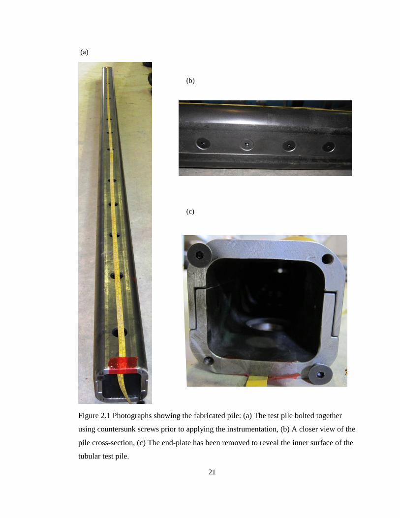
Figure 2.1 Photographs showing the fabricated pile: (a) The test pile bolted together using
countersunk screws prior to applying the instrumentation, (b) A closer view of the pile cross-
section, (c) The end-plate has been removed to reveal the inner surface of the tubular test pile. .. 21
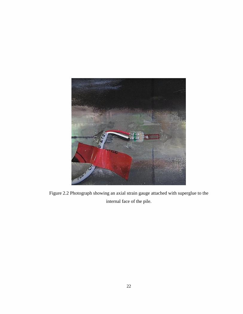
Figure 2.2 Photograph showing an axial strain gauge attached with superglue to the internal face
of the pile. ...................................................................................................................................... 22
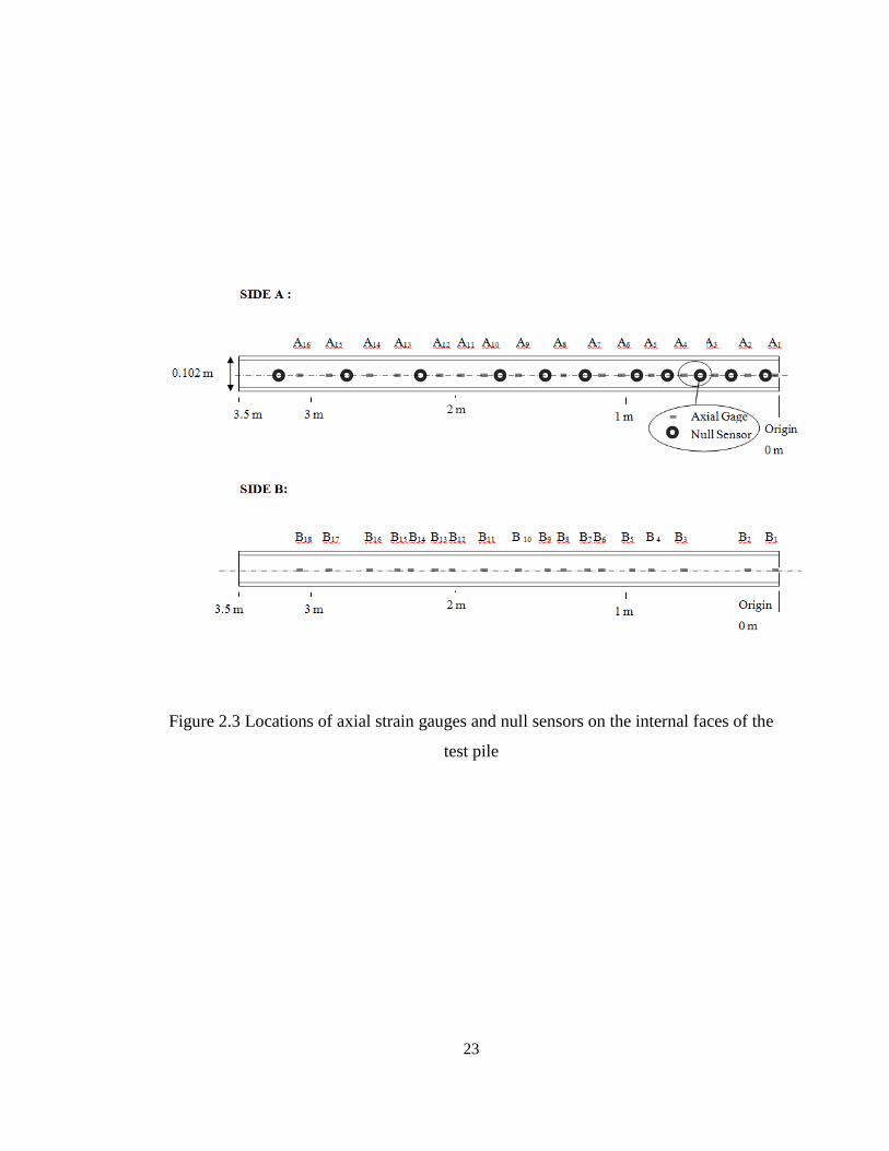
Figure 2.3 Locations of axial strain gauges and null sensors on the internal faces of the test pile 23
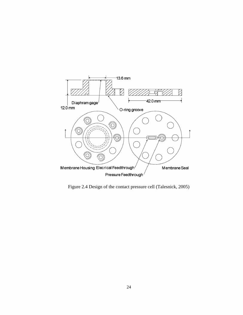
Figure 2.4 Design of the contact pressure cell (Talesnick, 2005) .................................................. 24
Figure 2.5 Location of null sensors along pile side A ................................................................... 25
Figure 2.6 Picture of the mounted steel bracket and two bolts used to hold the contact pressure
cell in place. ................................................................................................................................... 26
Figure 2.7 Photograph showing the beam test layout .................................................................... 27
Figure 2.8 Pressure reading versus time for bending Tests 1 and 2 ............................................... 28
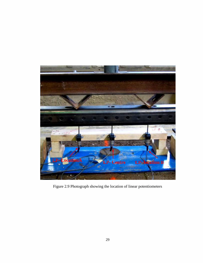
Figure 2.9 Photograph showing the location of linear potentiometers .......................................... 29
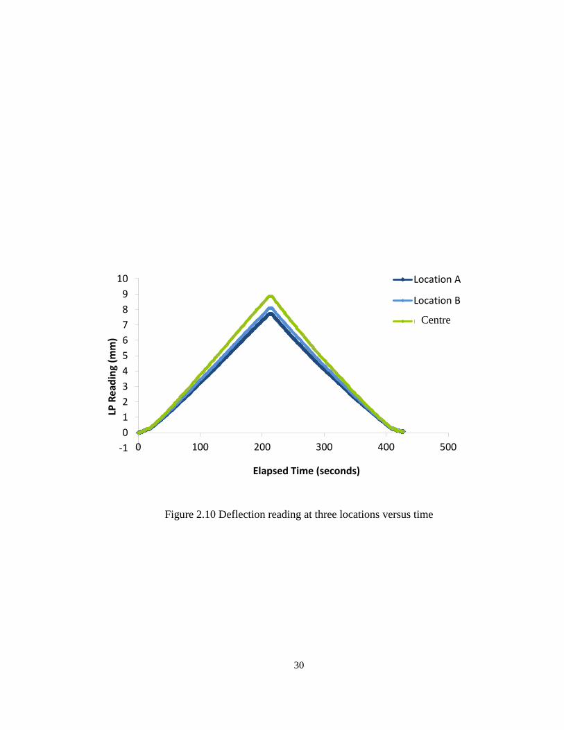
Figure 2.10 Deflection reading at three locations versus time ....................................................... 30
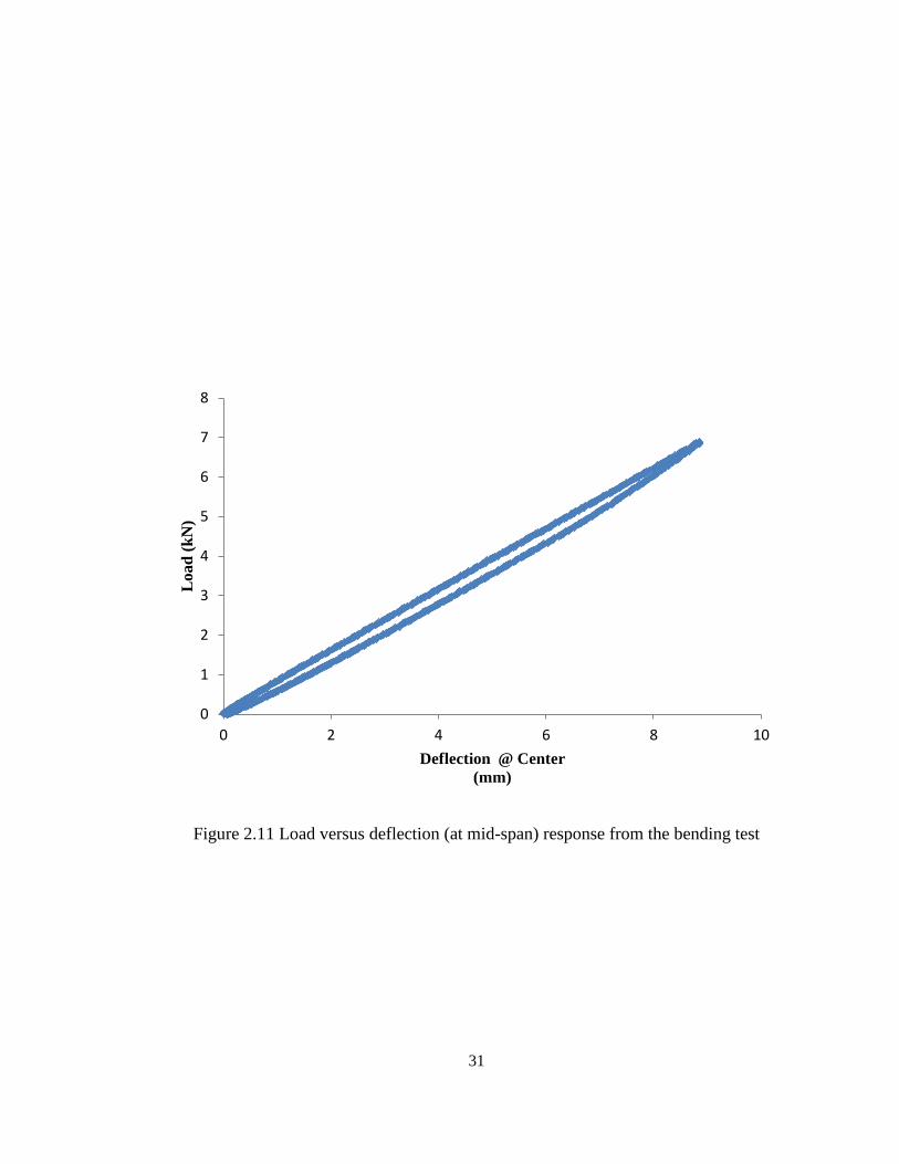
Figure 2.11 Load versus deflection (at mid-span) response from the bending test ....................... 31
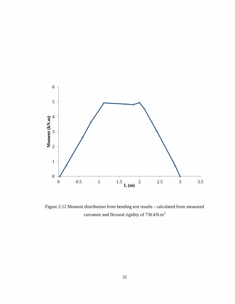
Figure 2.12 Moment distribution from bending test results - calculated from measured curvature
and flexural rigidity of 736 kN.m2 ................................................................................................. 32
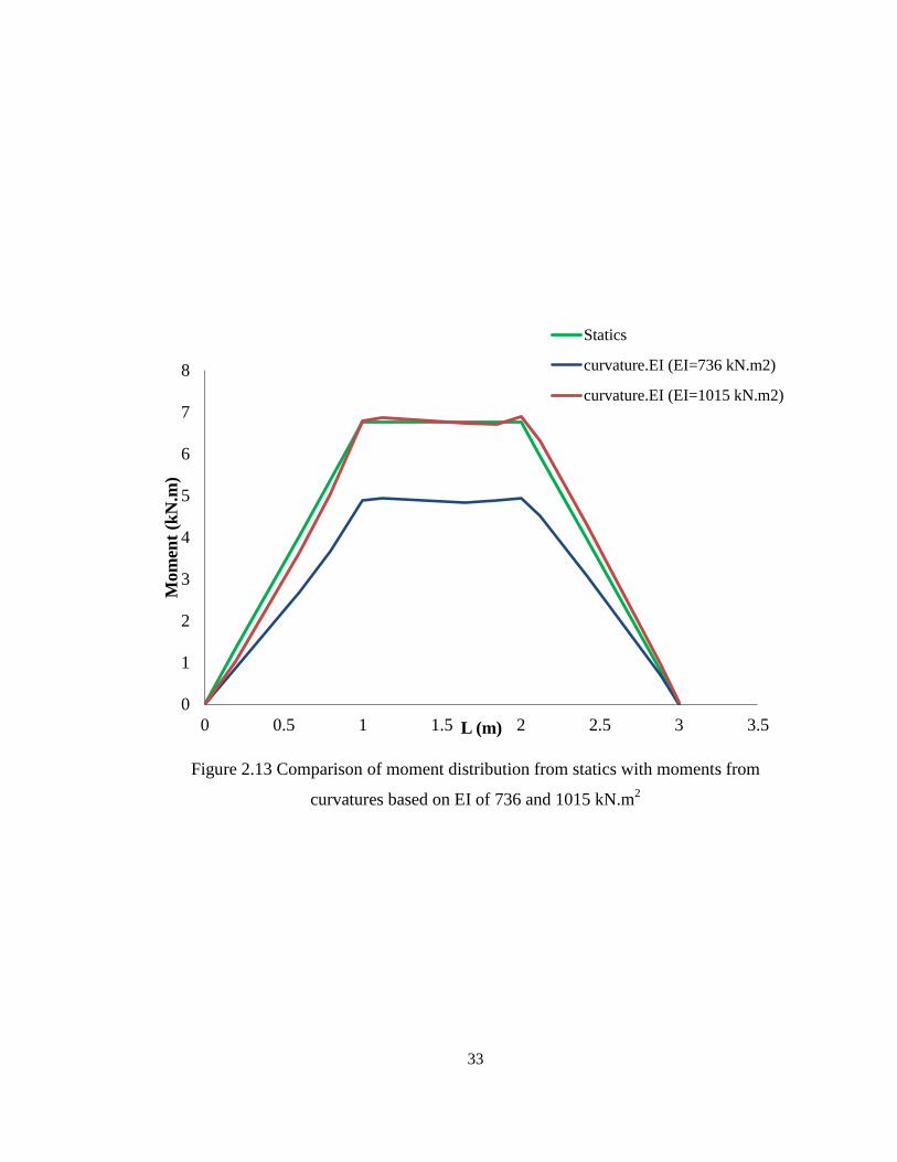
Figure 2.13 Comparison of moment distribution from statics with moments from curvatures based
on EI of 736 and 1015 kN.m2 ........................................................................................................ 33
Figure 3.1 Variation of Nq* with soil friction angle ϕ’ (After Meyehof, 1976). ........................... 46
Figure 3.2 Variation of end bearing resistance along the pile depth .............................................. 47
Figure 3.3 A Comparison between bearing capacity factor Nq* from selected theories for different
soil friction angle (Alawneh et al., 2001)....................................................................................... 48
Figure 3.4 Variation of shaft resistance along the embedment length of the pile. ......................... 49
Figure 3.5 Ultimate bearing capacity distribution ......................................................................... 50
Figure 3.6 Design approximations for free-head piles in a homogeneous soil (a) Ultimate lateral
resistance and bending moment for short piles(Poulos and Davis, 1980), (b) Ultimate lateral
resistance and bending moment for long piles (Poulos and Davis, 1980), (c) Ultimate lateral
resistance for free-head piles (Prasad and Chari, 1999). ................................................................ 51
Figure 3.7 Ultimate lateral load and moment capacity .................................................................. 52
ix
Figure 4.1 (a) Drawing showing the cross-sectional view of the test arrangement before pile
insertion. ........................................................................................................................................ 83
Figure 4.1 (b) Drawing showing the top view of the test pit. ........................................................ 84
Figure 4.2 Photograph showing the test pit while filling with Olivine sand. ................................. 85
Figure 4.3 The grain size distribution of Synthetic Olivine Sand. ................................................. 86
Figure 4.4 Photographs showing the fabricated test pile bolted together using countersunk screws
prior to applying the instrumentation, the end-plate has been removed to reveal the inner surface
of the pile. ...................................................................................................................................... 87
Figure 4.5 Locations of axial strain gauges and the null sensors along the pile. ........................... 88
Figure 4.6 Locations of null sensors along the pile length. ........................................................... 89
Figure 4.8 Static pile load tests layout. .......................................................................................... 91
Figure 4.9 Typical field load test system arrangement (England and Fleming, 2013). ................. 92
Figure 4.10 Photograph showing the test pile with a steel casing prior to insertion in to the soil
and once the casing is removed after insertion from static Test 2. ................................................ 93
Figure 4.11 Design of hollow steel pile driving frame. ................................................................. 94
Figure 4.12 Actuator applying lateral load to the test pile; load cell measured the applied force. 95
Figure 4.13 Maximum axial force distributions for axially loaded pile......................................... 96
Figure 4.14 Lateral soil pressure distributions for axially loaded pile at the end of pile installation.
....................................................................................................................................................... 96
Figure 4.15 Applied lateral load over the monitoring period......................................................... 97
Figure 4.16 Maximum bending moment distributions versus height above the pile toe for static
lateral load tests. ............................................................................................................................ 98
Figure 4.17 Static lateral load versus the measured deflection. ..................................................... 99
Figure 4.18 Soil pressure distributions for static lateral load tests (for lateral force=8 kN). ......... 99
Figure 4.19 Lateral force distributions per unit length for static tests ......................................... 100
(Uniform=Lateral pressure measurements from null sensors). .................................................... 100
Figure 4.20 Comparison of moment profile from statics (obtained by integrating lateral loads
along the pile) with measured moment for static Test 1. ............................................................. 101
Figure 4.21 Best fit polynomial for Moment Distribution, static lateral load Test 1. .................. 102
Figure 4.22 Comparison of soil pressure distributions from differentiation of moments and from
null sensors. ................................................................................................................................. 102
Figure 4.23 Pile deflection distribution for static lateral Test 1. .................................................. 103
Figure 5.1 Cyclic pile load tests layout. ....................................................................................... 127
Figure 5.2 Cyclic load responses in Tests 1 and 2. ...................................................................... 128
x
Figure 5.3 Cyclic load responses in Test 3. ................................................................................. 129
Figure 5.4 Cyclic load responses in Test 4. ................................................................................. 129
Figure 5.5 Cyclic load responses in Test 5. ................................................................................. 130
Figure 5.6 (a) Lateral load-deflection responses for cyclic Tests 1 and 2. .................................. 131
Figure 5.6 (b) Lateral load-deflection responses for cyclic Test 3. ............................................. 132
Figure 5.6 (c) Lateral load-deflection responses for cyclic Test 4. .............................................. 133
Figure 5.6 (d) Lateral load-deflection responses for cyclic Test 5. ............................................. 134
Figure 5.7 (a) Moment distributions for cyclic lateral load Tests 1 and 2 ................................... 135
(for lateral load = 8.0 kN) . .......................................................................................................... 135
Figure 5.7 (b) Moment distributions for cyclic lateral load Test 3, Two-way loading. ............... 136
Figure 5.7 (c) Moment distributions for cyclic lateral load Test 4, One-way loading. ................ 137
Figure 5.7 (d) Moment distributions for cyclic lateral load Test 5. ............................................. 138
Figure 5.8 (a) Earth pressure responses for cyclic load Tests 1 and 2 ......................................... 139
(for lateral load = 8.0 kN). ........................................................................................................... 139
Figure 5.8 (b) Earth pressure responses for cyclic load Test 3, Two-way loading. ..................... 140
Figure 5.8 (c) Earth pressure responses for cyclic load Tests 4, One-way loading. .................... 141
Figure 5.8 (d) Earth pressure responses for cyclic load Test 5. ................................................... 142
Figure 5.9 Photograph showing the pile-soil gap and heave occurred at the ground surface after
cyclic loading. .............................................................................................................................. 143
Figure 5.10 Bending moment distributions along the pile height above the toe for Tests 1 through
Test 5 (for lateral load =2.0 kN). ................................................................................................. 144
Figure 5.11 Lateral pressure distributions along the pile height above the toe for Tests 1 through
Test 5 (for lateral load =2.0 kN). ................................................................................................. 145
Figure A.1 Maximum axial force distributions for axially loaded pile Tests 1 to 4 .................... 155
Figure A.2 Maximum axial force distributions for axially loaded pile Test 5 ............................. 155
Figure A.3 Bending moment distributions along the axially loaded pile at the end of installation
..................................................................................................................................................... 156
Figure A.4 Pressure distributions for axially loaded pile at the end of installation ..................... 156
xi
List of Tables
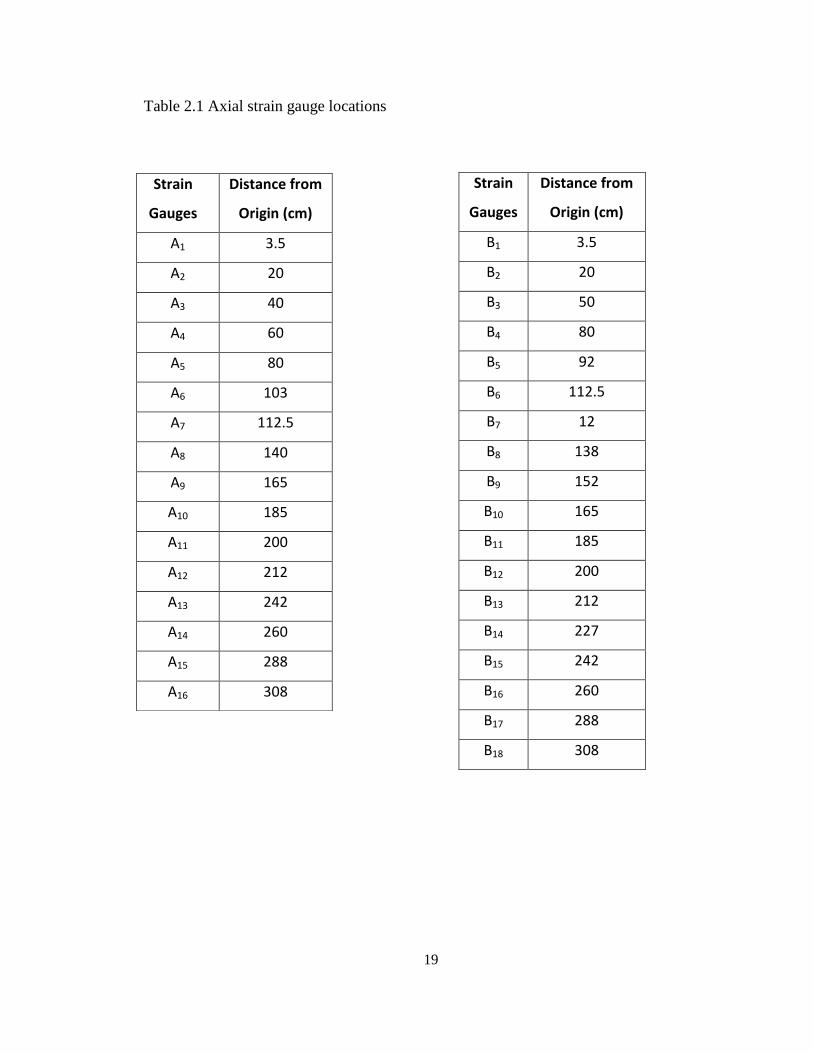
Table 2.1 Axial strain gauge locations ........................................................................................... 19
Table 2.2(a) Strain readings for bending Test 1 ............................................................................. 20
Table 2.2(b) Strain readings for bending Test 2 ............................................................................ 20
Table 3.1 Ultimate end bearing capacity along the embedded pile length .................................... 45
Table 3.2 Shaft resistance along the embedment length of the pile. .............................................. 45
Table 3.3 Ultimate bearing capacity. ............................................................................................. 45
Table 3.4 Theoretical ultimate lateral resistance and bending moment. ........................................ 45
Table 4.1 Axial Strain gauge locations .......................................................................................... 82
Table 5.1 Test layout for cyclic pile load tests ............................................................................ 126
Table 5.2 The null sensors calibration factors ............................................................................. 126
xii
List of Abbreviations
Ap Cross-sectional area of the pile
a Distance from the extreme fibre to the neutral axis
D Diameter of the pile
e Eccentricity from ground surface to applied load
E Modulus of elasticity
EI Flexural rigidity
f Distance below the ground surface where maximum moment occurs
F Applied force
F.O.S Factor of Safety
fs Unit friction resistance
H Applied lateral force,
Hu Ultimate lateral resistance
I Moment of inertia
K Effective earth pressure coefficient
Kp Coefficient of passive earth pressure
L Length of pile
M Moment
Nq* Bearing capacity factor
p Perimeter of pile
xiii
p(z) Lateral soil pressure in terms of pile height above the toe
Pa Atmospheric pressure
q' Effective vertical stress
ql Limiting point resistance
Qp Point resistance
Qs Shaft resistance and
Qu Ultimate bearing capacity
W Weight
y(z) deflection in terms of pile height above the toe
γ Unit weight of the soil
δ Displacement
δ'
Soil-pile friction angle
εc Compressive strain before yielding
εt Tensile strain before yielding
σoʹ Effective vertical stress
ϕ' Soil friction angle
Ψ Curvature
1
Chapter 1
INTRODUCTION
1.1 GENERAL
The use of pile foundations is perhaps the oldest method of constructing structures on soft
soils. Piles are stiff members that are generally made of steel, concrete, or timber. Once
installed, these geotechnical structures are used to transmit surface loads to a strong soil
layer at depth (end-bearing piles) or to spread the loads through the soil (floating piles)
when surface soils are soft or too loose to a support shallow foundation safely and
economically (Das, 2007). The load transfer mechanism from a pile to the soil is a
complex function of soil stratigraphy, pile geometry, loading position and soil properties
such as density and modulus. Therefore, pile load tests may be conducted in the design
phase of major construction projects to prove the suitability of the pile foundation system.
Pile foundations used in onshore and offshore structures are frequently subjected to static
and cyclic lateral loading such as wave action, ship impacts and wind loads (Qin and
Guo, 2007). The prediction of pile responses under axial and lateral forces has been the
subject of many research studies using theoretical approaches(Vesic, 1963; Janbu, 1976;
Kulhawy, 1984; Poulos, 1989). Though these studies are valuable for investigating pile
behaviour in foundation design, evaluation against measurements is required so their
performance can be assessed and improvements made to produce even better design
2
models. Therefore, this thesis describes the experimental responses of a vertical pile
embedded in dry sand when subjected to static and cyclic lateral loadings.
Two primary forms of instrumentation were used in the test pile to monitor response.
First, a series of axial strain gauges were employed from which to calculate curvature
under lateral load, and then moment distributions. Second, the test pile included a series
of lateral pressure sensors called ‘null gauges’ developed by Talesnick (2005) to record
the distribution of lateral earth pressures on the pile. What differentiates the current study
from previous investigations is the integration of direct measurements of lateral earth
pressure on a test pile using those ‘null’ sensors with conventional measurements of
curvature and deformation. The flush mount null sensors of Talesnick (2005) have
‘infinite stiffness’ and calibration that is almost independent of the soil type, soil
condition and stress history, qualities that make the sensor superior to other commercially
available sensors (Talesnick, 2005). These measurements are used to record the static and
cyclic pile responses under lateral loading.
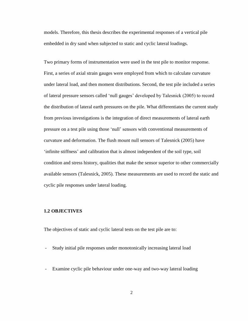
1.2 OBJECTIVES
The objectives of static and cyclic lateral tests on the test pile are to:
- Study initial pile responses under monotonically increasing lateral load
- Examine cyclic pile behaviour under one-way and two-way lateral loading
3
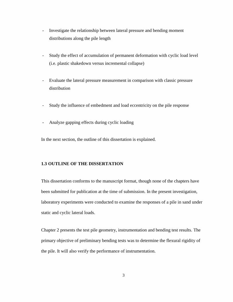
- Investigate the relationship between lateral pressure and bending moment
distributions along the pile length
- Study the effect of accumulation of permanent deformation with cyclic load level
(i.e. plastic shakedown versus incremental collapse)
- Evaluate the lateral pressure measurement in comparison with classic pressure
distribution
- Study the influence of embedment and load eccentricity on the pile response
- Analyze gapping effects during cyclic loading
In the next section, the outline of this dissertation is explained.
1.3 OUTLINE OF THE DISSERTATION
This dissertation conforms to the manuscript format, though none of the chapters have
been submitted for publication at the time of submission. In the present investigation,
laboratory experiments were conducted to examine the responses of a pile in sand under
static and cyclic lateral loads.
Chapter 2 presents the test pile geometry, instrumentation and bending test results. The
primary objective of preliminary bending tests was to determine the flexural rigidity of
the pile. It will also verify the performance of instrumentation.
4
The first strategy to determine pile behaviour is to take a theoretical approach. Chapter 3
focuses on the theoretical predictions of load capacities during axial and lateral loading.
The axial capacity of a pile installed into sand is expressed as the sum of the point and
shaft resistances. However, there are arguments about the accuracy of bearing capacity
design estimations from different methods. Additionally, the ultimate lateral capacity of
test pile, which is one of the key factors for design of offshore structures and structures in
earthquake zones, is predicted and explained in this chapter.
Chapter 4 and Chapter 5 describe static and cyclic pile load test results, respectively. In
each chapter, the test layout and loading procedures are explained in detail. Limitations
for the test layout for pile installation and lateral loading are presented in Chapter 4.
Although the main goal of this work was to examine pile responses under lateral loading,
the axial responses during pile installation were recorded and are presented briefly. In
Chapter 4, the lateral responses of the fabricated pile including bending moment, lateral
pressure and deflection distributions are analyzed. The results from the static pile load
tests are compared and evaluated against existing design methods.
Chapter 5 deals with the pile response under lateral loading for five cyclic loading tests.
In these tests, the cyclic loadings were applied under different conditions to examine the
impact of embedment, load eccentricity, loading type (one-way versus two-way) and
repeated cycles on pile behaviour.
At the end, Chapter 6 provides the summary and conclusions of Chapters 2 through 5.
5
1.4 REFERENCES
Das, B.M., 2007, Principles of Foundation Engineering. Sixth Edition, Thomson Canada
Limited, pp. 310-319.
Talesnick, M., 2005, Measuring Soil Contact Pressure on a Solid Boundary and
Quantifying Soil Arching. Geotechnical Testing Journal, Vol. 28, No. 2, pp. 1-9.
Qin, H. and Guo, W.D., 2007, An Experimental Study on Cyclic Loading of Piles in
Sand. Griffith University, Australia.
6
Chapter 2
TEST PILE GEOMETRY, INSTRUMENTATION AND BENDING
TEST RESULTS
2.1 INTRODUCTION
Many structures, specifically in a soft soil, are often supported on piles. Pile foundations
are subjected to axial and lateral loading and they transfer the load to bearing strata with
greater bearing capacity (Orfano, 2009). Therefore, pile foundations must be designed
and tested to resist both axial and lateral forces.
Before conducting the pile load tests, beam tests were conducted on the test pile. The
main objective of the pile bending experiments is to determine the value of flexural
rigidity (EI) so that test measurements of extreme fibre strain and curvature calculated
from strain, can then be used to calculate longitudinal bending moments. In addition, a
suitable for of EI is needed for use in determining deflections by integrating moments.
Finally, the bending tests were conducted to confirm that all the instrumentation was
performing correctly and providing consistent readings. This chapter describes the
fabricated test pile design, instrumentation and the results of the preliminary bending
tests.
2.2 TEST PILE GEOMETRY AND INSTRUMENTATION
The tests were performed on a hollow square steel tube with nominal size of
HSS102x102x13 mm, which was fabricated from two sections cut from an HSS of
7
dimensions 152x102x13. The properties and design data of the pile are available in detail
in the Canadian Institute of Steel Construction Manual (2007). The length of the test pile
is 3.5 m and mass is 108 kg. The rectangular steel tube was cut into two ‘C-sections’ with
flanges cut so they overlap. These flanges were then fitted with a series of regularly
spaced bolts with countersunk heads to join the two halves of the test pile after installing
the instrumentation along its inner surface. Figure 2.1 presents images of the fabricated
pile bolted together taken from different views.
The two main instruments used to measure the pile response are strain gauges and null
sensors. It is common practice in pile load testing for research studies to monitor the axial
strains along the pile and calculate the bending moment from the measured strains. To
estimate the moment distribution, thirty-four (34) axial strain gauges were attached with
Cyanoacrylate (superglue) to the internal faces of the pile along the length at
approximately 0.2 m intervals. Figure 2.2 shows a photograph of an axial strain gauge
attached with Cyanoacrylate to the internal face of the pile. Sixteen gauges were installed
on one half of the test pile (Pile Side A) and the remaining eighteen gauges were installed
on the other half (Pile Side B). The intervals at which the axial strain gauges were
attached are given in Table 2.1 and their axial locations and their positions within the pile
cross-section are shown in Figure 2.3.
Another key objective of this test program on laterally loaded piles was to measure the
distribution of lateral earth pressure on the test pile. Special contact pressure sensors
called “null sensors” have recently been developed by Talesnick (2005). These were
mounted along the pile to determine the lateral earth pressures acting on the test pile.
8
Figure 2.4 shows the component of the contact pressure sensor and its dimension. The
sensor has two parts: a membrane face which is mounted flush to the soil-structure
boundary and a housing back which is a cylindrical volume behind the membrane face. A
quarter-bridge foil diaphragm strain gauge is attached under the membrane face. The
thickness of the sensor is 44.5 mm with a membrane face of diameter 52.5 mm
(Talesnick, 2005).
The sensor is operating based on the null method. When the soil pressure is applied on
the outer surface of the membrane, air pressure in the cylindrical volume is adjusted
through digital control to return the diaphragm strain gauge to its un-deformed position,
making the sensor act as though it were rigid. This eliminates most of the calibration
issues that are known to make earth pressure measurement challenging (Talesnick, 2005).
The applied air pressure is calibrated to be equal to the soil pressure on the outer
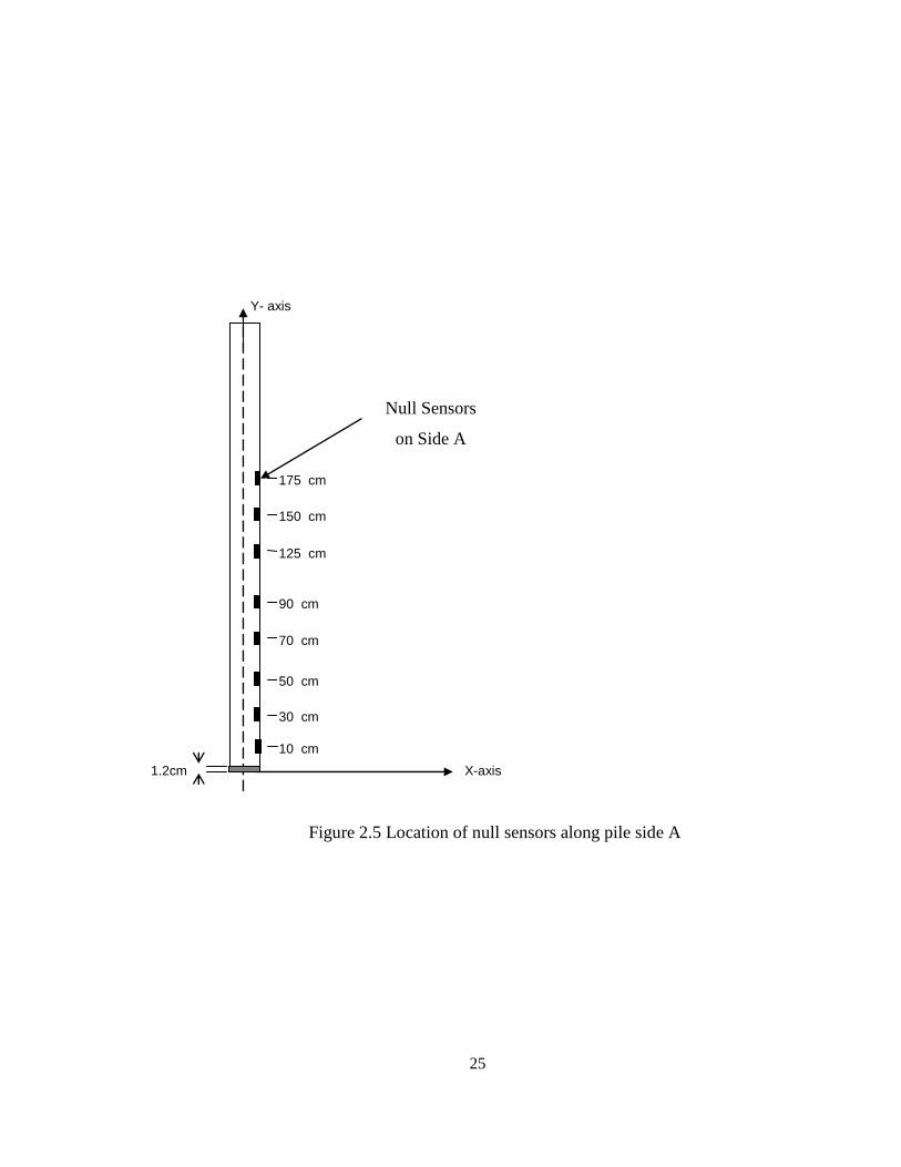
membrane face (Talesnick, 2005). Seven null sensor holes were located on one side of
the pile (six null sensors were available for use in the project). The locations of the sensor
holes along the model pile are shown in Figure 2.5.
To hold the sensors in place and maintain zero pressure reading during bending tests (to
ensure that the sensor’s membrane does not stretch or compress as tensile or compressive
strains develop in the steel test pile), steel brackets bolted to the pile above the null sensor
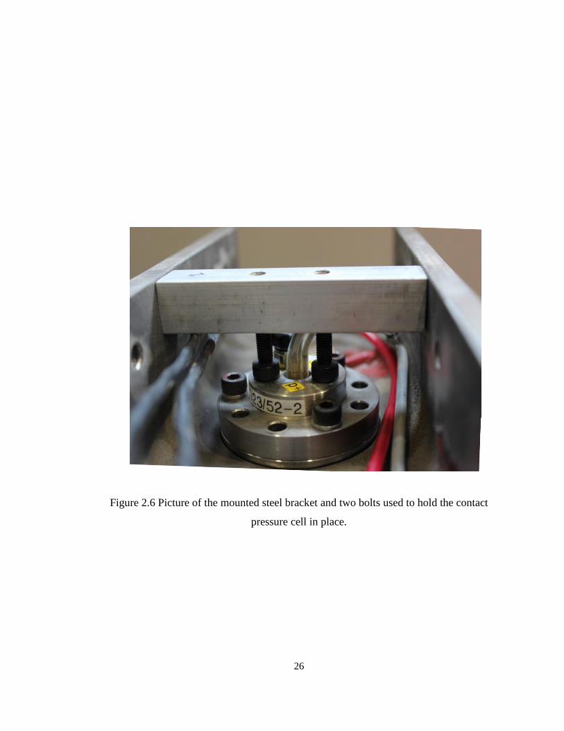
were used to hold it in place (the sensor was not fastened directly to the test pile). The
brackets are 76 mm long with square cross section of 20 mm x 20 mm. Two screws, with
nominal size M5x2, extend from the bracket to touch the rear surface of the null sensor
and hold it in position within the circular hole that accommodates it in the test pile,
9
Figure 2.6. The brackets are not screwed to the sensors, but simply held to prevent them
moving towards the central axis of the test pile. This method of holding the sensors in
position is employed instead of bolting the null sensor to the test pipe, since it prevents
strains developing in the sensors during bending.
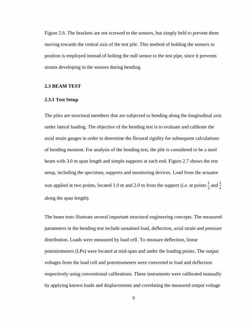
2.3 BEAM TEST
2.3.1 Test Setup
The piles are structural members that are subjected to bending along the longitudinal axis
under lateral loading. The objective of the bending test is to evaluate and calibrate the
axial strain gauges in order to determine the flexural rigidity for subsequent calculations
of bending moment. For analysis of the bending test, the pile is considered to be a steel
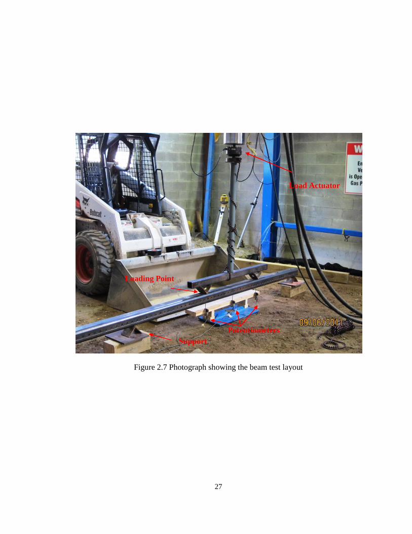
beam with 3.0 m span length and simple supports at each end. Figure 2.7 shows the test
setup, including the specimen, supports and monitoring devices. Load from the actuator
was applied at two points, located 1.0 m and 2.0 m from the support (i.e. at points
and
along the span length).
The beam tests illustrate several important structural engineering concepts. The measured
parameters in the bending test include sustained load, deflection, axial strain and pressure
distribution. Loads were measured by load cell. To measure deflection, linear
potentiometers (LPs) were located at mid-span and under the loading points. The output
voltages from the load cell and potentiometers were converted to load and deflection
respectively using conventional calibrations. These instruments were calibrated manually
by applying known loads and displacements and correlating the measured output voltage
10
against the known values. All the instrumentation was connected to the data acquisition
system which consists of a data-logger and computer. The strain gauges were hooked into
a System 5000 controlled using Strain Smart software. The null gauges were controlled
using a National Instruments data acquisition platform using software adapted by
Andreae (2010) from the original control systems developed by Talesnick. For a given
applied load, the pile responses at all the instrumentation locations including strain
gauges, null sensors and linear potentiometers were measured and stored. To confirm the
results, the bending tests were conducted twice: Bending Test 1, when the load is applied
on pile side A, and Bending Test 2, when the load is applied on pile side B.
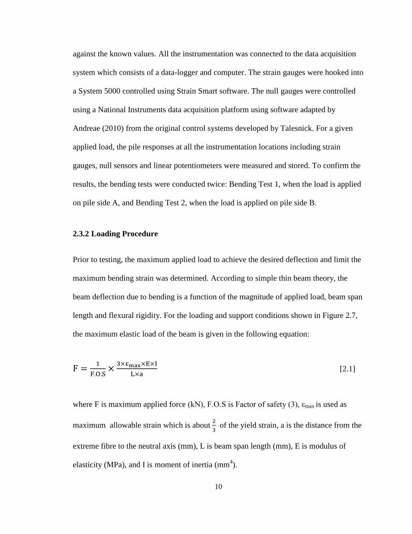
2.3.2 Loading Procedure
Prior to testing, the maximum applied load to achieve the desired deflection and limit the
maximum bending strain was determined. According to simple thin beam theory, the
beam deflection due to bending is a function of the magnitude of applied load, beam span
length and flexural rigidity. For the loading and support conditions shown in Figure 2.7,
the maximum elastic load of the beam is given in the following equation:
[2.1]
where F is maximum applied force (kN), F.O.S is Factor of safety (3), εmax is used as
maximum allowable strain which is about
of the yield strain, a is the distance from the
extreme fibre to the neutral axis (mm), L is beam span length (mm), E is modulus of
elasticity (MPa), and I is moment of inertia (mm4).
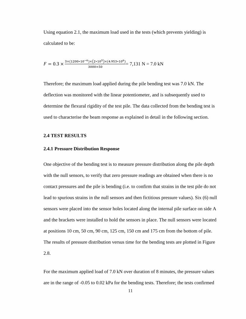
11
Using equation 2.1, the maximum load used in the tests (which prevents yielding) is
calculated to be:
( )
= 7,131 N = 7.0 kN
Therefore; the maximum load applied during the pile bending test was 7.0 kN. The
deflection was monitored with the linear potentiometer, and is subsequently used to
determine the flexural rigidity of the test pile. The data collected from the bending test is
used to characterise the beam response as explained in detail in the following section.
2.4 TEST RESULTS
2.4.1 Pressure Distribution Response
One objective of the bending test is to measure pressure distribution along the pile depth
with the null sensors, to verify that zero pressure readings are obtained when there is no
contact pressures and the pile is bending (i.e. to confirm that strains in the test pile do not
lead to spurious strains in the null sensors and then fictitious pressure values). Six (6) null
sensors were placed into the sensor holes located along the internal pile surface on side A
and the brackets were installed to hold the sensors in place. The null sensors were located
at positions 10 cm, 50 cm, 90 cm, 125 cm, 150 cm and 175 cm from the bottom of pile.
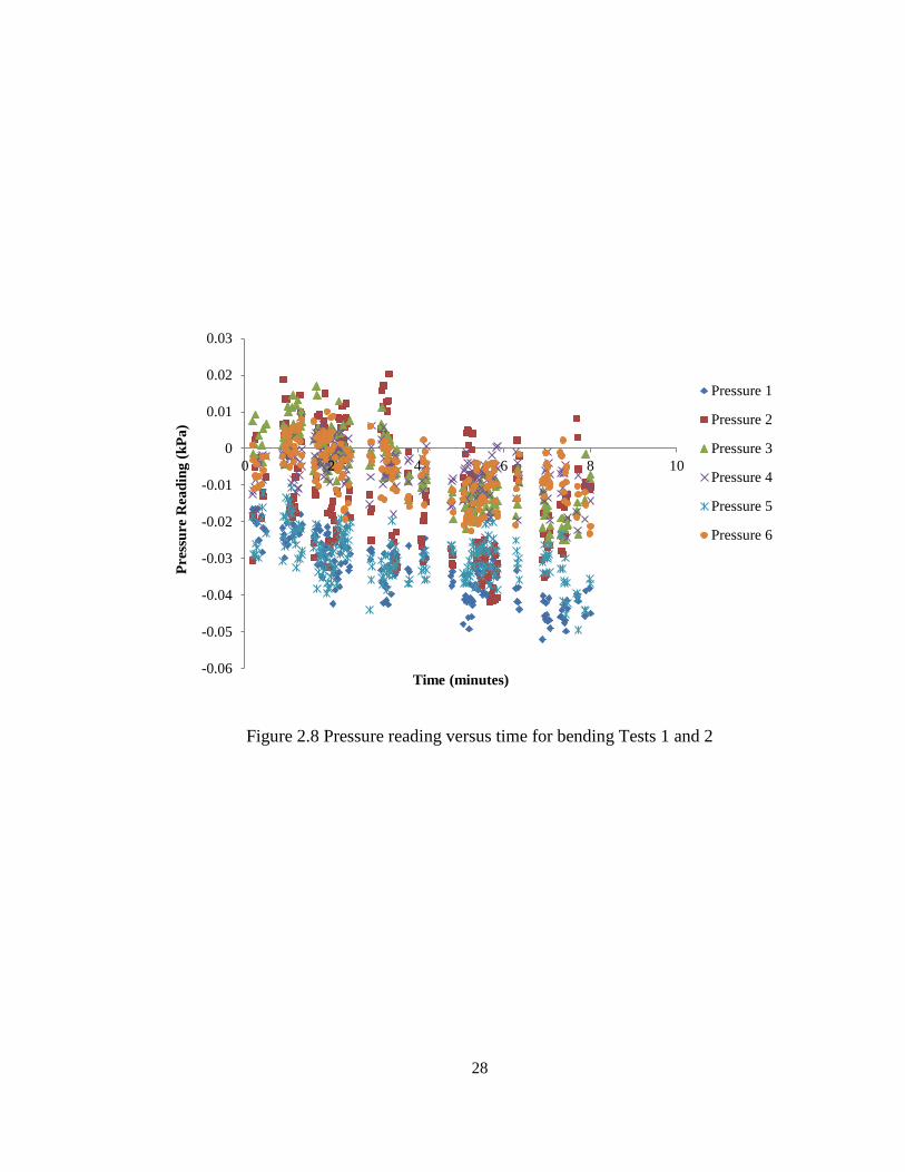
The results of pressure distribution versus time for the bending tests are plotted in Figure
2.8.
For the maximum applied load of 7.0 kN over duration of 8 minutes, the pressure values
are in the range of -0.05 to 0.02 kPa for the bending tests. Therefore; the tests confirmed
12
approximately zero pressure readings in the case of pile bending without contact
pressures.
2.4.2 Deflection-Time Response
Linear potentiometers were located at three different locations: mid-span (denoted LP
Centre) and under the loading points at 1 m and 2 m from the supports (LP A and LP B),
as presented in Figure 2.9. The recorded deflections over the monitoring period were
plotted for each location, as shown in Figure 2.10.
From Figure 2.10, it is seen that no residual displacement was measured at any of the
linear potentiometers. A maximum deflection of 9 mm was observed at the centre of the
pile span. The linear potentiometer readings under the loading points at locations A and B
were expected to be same. However, they were somewhat different, though with
maximum discrepancy of less than 0.5 mm. The minor deflection differences are likely a
result of the changes in pile stiffness associated with the perforations made in one face of
the pile to accommodate the pressure sensors, but might also be due to sensor precision
and calibration error. Other possible reasons for this discrepancy could be settlement of
the soil since the bending tests were performed with the supports holding the test pile
resting on the soil, or a soil surface that was not perfectly leveled prior to testing.
2.4.3 Load-Deflection Response
By plotting load-deflection response, the stiffness of a given material is determined. With
the help of the data-logger, the results are plotted while the test is running. Load-
deflection plots were monitored to "ensure the beam is not loaded beyond the elastic
13
limit, indicated by a reduction in the slope" (Matsumoto et al., 2001).In addition, the
residual displacement was verified upon unloading.
The material stiffness of steel beam is measured from the slope of the load-deflection
diagram given in the following equation:
[2.2]
where ∆F is the change in Force (N), ∆δ is the change in deflection (mm) and material
stiffness (N/mm).
Figure 2.11 shows the plot of load versus deflection at the mid-span where the maximum
deflection occurs. The plot verifies linear elastic behaviour given that the slope is linear
during a loading-unloading cycle and the deflection value returns to almost zero when the
beam is unloaded. For the case of linear elastic behaviour, the material stiffness is
calculated from the slope of the load-deflection curve by plotting a linear trend line. The
result shows that the maximum applied load is 7.0 kN and the corresponding deflection is
8.9 mm, as shown in Figure 2.11.
2.4.4 Flexural Rigidity
Flexural rigidity of a beam cross section is defined by EI, where E is the modulus of
elasticity and I is the moment of inertia of the beam (i.e. the test pile). First, the flexural
rigidity for an intact hollow section with the same cross-sectional geometry is estimated
from the Canadian Institute of Steel Construction (CISC) (2007). The moment of inertia
(I) of 102x102x13 mm steel pile is 495.3x104 mm
4 and the modulus of elasticity of steel
14
(Esteel) is 200 GPa. Using these two parameters, the flexural rigidity of an intact section is
990 kN.m2.
To determine the flexural rigidity of the beam from the bending test results, the following
equation is rearranged, where F is the maximum applied force and δ is the measured
deflection at the loading points corresponding to maximum load during the bending tests.
[2.3]
EI is calculated from the measurements to be 728 kN.m2 for bending Test 1 and 744
kN.m2 for bending Test 2.
The flexural rigidity of the test pile from deflection results is calculated to be 736 kN.m2
(the average of the calculated EI values from Tests 1 and 2). The reason for estimating a
different value of flexural rigidity is likely because the test pile has been perforated to
install the contact pressure sensors. Those perforations are on the extreme fiber and so
likely are the primary reason for the reduction of total flexural stiffness by 27%. Another
possible reason for reduced stiffness is assembly from two C-sections screwed together
with a series of bolts. The moment of inertia for the fabricated test pile may not then be
the same as the original hollow structural section. In addition, there may be deformation
across the joints as shear stress is transferred from one segment to the other. In the next
section, there is evidence that the first explanation (perforation) is the primary reason for
reduced stiffness.
15
2.4.5 Bending Moment Distribution
This section discusses the basic beam behaviour that occurred during the bending test.
When a beam is subjected to a transverse load, it deflects into a curved shape. This will
cause the top surface of the beam where the load is applied to be in compression and the
bottom surface to be in tension. The bending produces strains with a tri-linear
relationship (i.e. three straight lines). The bending tests were conducted on both faces of
the pile where the strain gauges were attached (Side A and Side B). In bending Test 1, the
load was applied on pile side A and the pile was rotated 180 degrees to conduct bending
test 2 on side B.
The moment distribution developed during the bending test can be related to the strain
values measured by strain gauges along the pile length using the flexural rigidity.
According to Welch and Reese (1972), the relation between moment and bending strains
is as follow:
[2.4]
where Ψ =curvature, εt=tensile strain (+ve), εc= compressive strain (-ve) and d=the
distance between the two gauges.
As discussed earlier, thirty-four axial strain gauges were attached along the pile axis.
However, perhaps due to moisture under a few of the strain gauges after installation, the
readings for only twelve pairs of strain gauges were reliable throughout the tests. Tables
2.2 (a) and (b) present the measured strain values from the axial strain gauges along the
pile length for the maximum applied load. Table 2.2(a) shows the result for bending test 1
16
where the load is applied on pile side A. Therefore, strain gauges A1 to A16 are in
compression since these gauges are attached to the side where the load is applied and
strain gauges B1 to B18 are in tension. Loading was applied to the opposite side of the test
pile in bending test 2, and so strains reversed (tension for gauges A1 to A16, and
compression for gauges B1 to B16), as presented in Table 2.2(b).
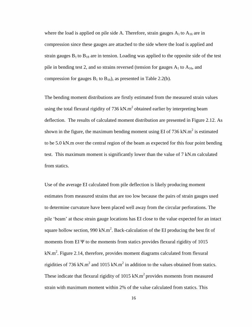
The bending moment distributions are firstly estimated from the measured strain values
using the total flexural rigidity of 736 kN.m2 obtained earlier by interpreting beam
deflection. The results of calculated moment distribution are presented in Figure 2.12. As
shown in the figure, the maximum bending moment using EI of 736 kN.m2 is estimated
to be 5.0 kN.m over the central region of the beam as expected for this four point bending
test. This maximum moment is significantly lower than the value of 7 kN.m calculated
from statics.
Use of the average EI calculated from pile deflection is likely producing moment
estimates from measured strains that are too low because the pairs of strain gauges used
to determine curvature have been placed well away from the circular perforations. The
pile ‘beam’ at these strain gauge locations has EI close to the value expected for an intact
square hollow section, 990 kN.m2. Back-calculation of the EI producing the best fit of
moments from EI to the moments from statics provides flexural rigidity of 1015
kN.m2. Figure 2.14, therefore, provides moment diagrams calculated from flexural
rigidities of 736 kN.m2 and 1015 kN.m
2 in addition to the values obtained from statics.
These indicate that flexural rigidity of 1015 kN.m2
provides moments from measured
strain with maximum moment within 2% of the value calculated from statics. This
17
flexural rigidity of 1015 kN.m2 will therefore be used to characterize local beam stiffness
employed in calculations of moment based on measured strain, whereas the average
flexural rigidity of 736 kN.m2 back-calculated from the beam deflections will be used in
estimations of deflection presented later in the thesis obtained by integrating moment
distribution along the pile.
2.5 SUMMARY
Many structures are supported by end-bearing piles to transmit the surface loads to the
stronger soil layers or floating piles to spread the loads through the soil safely and
economically. The main objective of this thesis is to study the behaviour of the fabricated
test pile under static and cyclic lateral loading in sand. However, prior to pile testing, the
performance of the instruments was examined by conducting beam bending tests.
Bending tests were performed to confirm that the pressure sensors do not provide
spurious readings when the pile is deformed and the strain gauges could be used to
determine accurate moment from measure strain. The tests verified that the null sensors
which were mounted to the internal face of the pile provide zero contact pressure in the
case of pile bending. In addition, accurate strain readings were measured with strain
gauges to obtain moment distribution.
The other objective of bending test was to determine the flexural rigidity of the fabricated
pile for use in interpreting pile bending tests presented in subsequent chapters. Local
stiffness of the test pile in the vicinity of the strain gauges is characterized using flexural
rigidity of 1015 kN.m2, and this value is subsequently used to calculate moments from
strains measured during the pile load tests. The average stiffness of the test pile (the value
18
controlling the flexural deflections) is characterized using flexural rigidity of 736 kN.m2,
and this is subsequently used to calculate pile deflections by integrating moments.
2.6 REFERENCES
Handbook of Steel Construction, 2007. Canadian Institute of Steel Construction (CISC).
Ninth Edition, Lakeside Group Inc, pp. 4-102. Retrieved February 25, 2013, from
http://www.engineersedge.com/manufacturing spec/properties of metals strengt
h.htm
Matsumoto, E., Johnston, R., Dammel, E., and Ramesh, S.K., 2001. A Simple Beam Test.
Proceedings of the 2001 American Society for Engineering Education Annual
Conference & Exposition, Sacramento.
Orfano, F., 2009, Pile Foundation. Retrieved 10 November, 2013, from
http://www.brighthubengineering.com/building-construction-design/45946-intro-
to-pile-foundation/
Talesnick, M., 2005. Measuring Soil Contact Pressure on a Solid Boundary and
Quantifying Soil Arching. Geotechnical Testing Journal, Vol. 28, No. 2, pp. 1-4.
19
Table 2.1 Axial strain gauge locations
Strain
Gauges
Distance from
Origin (cm)
A1 3.5
A2 20
A3 40
A4 60
A5 80
A6 103
A7 112.5
A8 140
A9 165
A10 185
A11 200
A12 212
A13 242
A14 260
A15 288
A16 308
Strain
Gauges
Distance from
Origin (cm)
B1 3.5
B2 20
B3 50
B4 80
B5 92
B6 112.5
B7 12
B8 138
B9 152
B10 165
B11 185
B12 200
B13 212
B14 227
B15 242
B16 260
B17 288
B18 308

20
Bending Test 1
Bending Test 2
Gauge
No. (Micro-Strain)
Gauge
No. (Micro-Strain)
A1 -5.71
A1 32.37
A2 -36.47
A2 41.68
A5 -184.62
A5 181.39
A7 -259.7
A7 255.13
A8 -99999
A8 -99999
A9 -247.72
A9 247.88
A10 -248.83
A10 251.37
A11 -260.7
A11 258.99
A12 -240.66
A12 234.64
A13 -158.94
A13 159.48
A14 -99999
A14 -99999
A15 -34.61
A15 34.61
A16 -3.79
A16 -4.27
B1 -99999
B1 -99999
B2 46.14
B2 -35.67
B3 153.17
B3 -140.79
B4 208.11
B4 -198.51
B6 259.13
B6 -260.87
B8 254.23
B8 -255.49
B10 209.79
B10 -259.14
B11 216.37
B11 -252.33
B12 252.44
B12 -258.46
B13 227.21
B13 -238.93
B15 162.8
B15 -161.3
B17 39.98
B17 -39.5
B18 -1.42
B18 -8.07
Table 2.2(a) Strain readings for
bending Test 1
Table 2.2(b) Strain readings for
bending Test 2
21
(a)
(b)
(c)
Figure 2.1 Photographs showing the fabricated pile: (a) The test pile bolted together
using countersunk screws prior to applying the instrumentation, (b) A closer view of the
pile cross-section, (c) The end-plate has been removed to reveal the inner surface of the
tubular test pile.
22
Figure 2.2 Photograph showing an axial strain gauge attached with superglue to the
internal face of the pile.
23
Figure 2.3 Locations of axial strain gauges and null sensors on the internal faces of the
test pile
24
Figure 2.4 Design of the contact pressure cell (Talesnick, 2005)
25
0.1
Null Sensors
on Side A
X-axis
1.2cm
Y- axis
10 cm
70 cm
50 cm
30 cm
90 cm
125 cm
150 cm
175 cm
Figure 2.5 Location of null sensors along pile side A
26
Figure 2.6 Picture of the mounted steel bracket and two bolts used to hold the contact
pressure cell in place.
27
Figure 2.7 Photograph showing the beam test layout
Load Actuator
Potentiometers
Loading Point
Support
28
Figure 2.8 Pressure reading versus time for bending Tests 1 and 2
-0.06
-0.05
-0.04
-0.03
-0.02
-0.01
0
0.01
0.02
0.03
0 2 4 6 8 10
Pre
ssu
re R
ead
ing
(k
Pa
)
Time (minutes)
Pressure 1
Pressure 2
Pressure 3
Pressure 4
Pressure 5
Pressure 6
29
Figure 2.9 Photograph showing the location of linear potentiometers
LP- LocationA
A
LP- location B LP- Centre
30
Figure 2.10 Deflection reading at three locations versus time
-1
0
1
2
3
4
5
6
7
8
9
10
0 100 200 300 400 500
LP R
ead
ing
(mm
)
Elapsed Time (seconds)
Location A
Location B
CenterCentre
31
Figure 2.11 Load versus deflection (at mid-span) response from the bending test
0
1
2
3
4
5
6
7
8
0 2 4 6 8 10
Load
(k
N)
Deflection @ Center
(mm)
32
Figure 2.12 Moment distribution from bending test results - calculated from measured
curvature and flexural rigidity of 736 kN.m2
0
1
2
3
4
5
6
0 0.5 1 1.5 2 2.5 3 3.5
Mom
ent
(kN
.m)
L (m)
33
Figure 2.13 Comparison of moment distribution from statics with moments from
curvatures based on EI of 736 and 1015 kN.m2
0
1
2
3
4
5
6
7
8
0 0.5 1 1.5 2 2.5 3 3.5
Mom
ent
(kN
.m)
L (m)
Statics
curvature.EI (EI=736 kN.m2)
curvature.EI (EI=1015 kN.m2)
34
Chapter 3
THEORETICAL PREDICTIONS OF AXIAL AND LATERAL LOAD
CAPACITIES
3.1 INTRODUCTION
Structures supported by piled foundations can be subjected to axial and lateral loadings.
Examples of the applied loads on a piled foundation include dead and live loads from the
structure, wind forces, earthquakes, ship impacts and wave actions. Expected pile
deformations under service loads and their ultimate load capacity are controlling factors
in foundation design. Pile load tests can be conducted to determine the ultimate bearing
capacity or the deflection of the pile at the service load.
Although pile foundations have been used in construction for many years, it was only in
the 1960’s that rational procedures for estimating pile strength and deformations were
established. There are several methods for calculating the bearing capacity of foundations
including theoretical static analysis (Vesic, 1963; Janbu, 1976; Kulhawy, 1984; Poulos,
1989), procedures based on in situ test results (Meyerhof, 1976; Schmertmann, 1978;
Eslami. 1995 and Fellenius, 1997), dynamic methods (Goble et al., 1979; Rausche et al.,
1985; Fellenius, 2006) and finally from interpretation of full scale pile load tests
(Fellenius, 1990).The first design strategy is often chosen to be the theoretical approach
since the other design strategies are sometimes time consuming and costly (Vieskarami et
al., 2011). Therefore, the first step in this research is to estimate the axial and lateral load
35
capacities of a pile using the theoretical approaches which are explained in the following
sections.
3.2 AXIAL CAPACITY
The behaviour of pile foundations subjected to axial loading is complex since it alters the
state of stress in the ground. Understanding the behaviour of piles during installation and
loading requires high-quality test data on instrumented piles. In the past, pile
instrumentation was unable to withstand high driving stresses and provide reliable
residual stresses. Iskander (2010) noted that residual stresses are a significant component
of shaft resistance capacity and may influence the stress distribution along the pile during
loading. Therefore, well-established analytical methods were developed for estimating
axial pile capacity in cohesive and cohesionless soil.
The axial load capacity of a pile is derived from friction along the pile shaft and
resistance at the pile tip. This section describes the axial capacity of a displacement pile
in sand using theoretical predictions.
The ultimate bearing capacity Qu of a pile installed into sand can be expressed as the sum
of the point resistance Qp, shaft resistance Qs and weight of the displaced soil (Wdisplaced
soil), minus the weight of the pile (Wpile), as follows:
Qu= Qp + Qs+ Wdisplaced soil - Wpile [3.1]
where weight of the displaced soil is the soil unit weight (γsoil) multiplied by the volume
of the buried pile, and weight of the pile with the same cross-sectional geometry, which is
36
estimated from the Canadian Institute of Steel Construction (2007). Different studies
have been conducted to determine the values of Qp and Qs. The axial load capacity is
computed based on the unit shaft and toe resistances. Vesic and Meyehof (1963 and
1964) introduced the concept of critical depth or limiting values of shear stress along the
shaft, increasing with depth, but only up to a maximum or “limiting value” (Kerisel 1961,
Vesic 1963, Hanna and Tan 1973, Das and Seeley 1975, Tavenas 1971, after Kraft et al.
1991).The following section discusses the calculation of end bearing and shaft resistances
in detail.
3.2.1 End Bearing Resistance, Qp
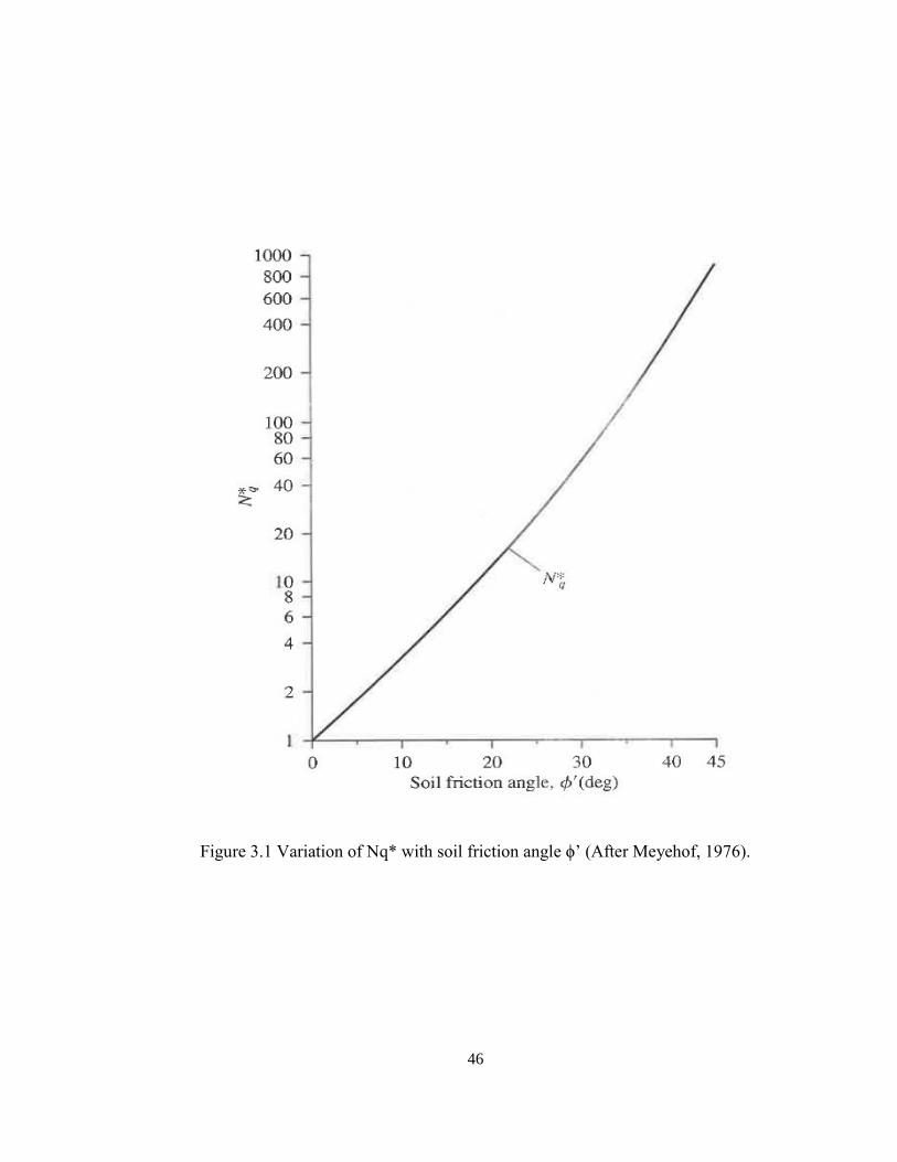
Meyerhof (1976) suggested the ultimate end bearing or point resistance of piles in
homogenous sand is obtained from the following equations:
Qp = Apq'Nq* ≤ Apql [3.2]
where Ap is the area of pile toe, q' is the effective vertical stress at the level of the pile toe
and Nq* is the bearing capacity factor obtained from Figure 3.1 which shows the
variation of Nq* with soil friction angle ϕ' (Das, 2007). ql is the limiting point resistance
computed from Equation 3.3.
ql = 0.5 PaNq*( tanϕ' ) [3.3]
where Pa , the atmospheric pressure, is 100 kN/m2. This method assumes that the point
bearing capacity of a pile increases linearly with depth, but reaches a limiting value of ql
beyond a certain depth.
37
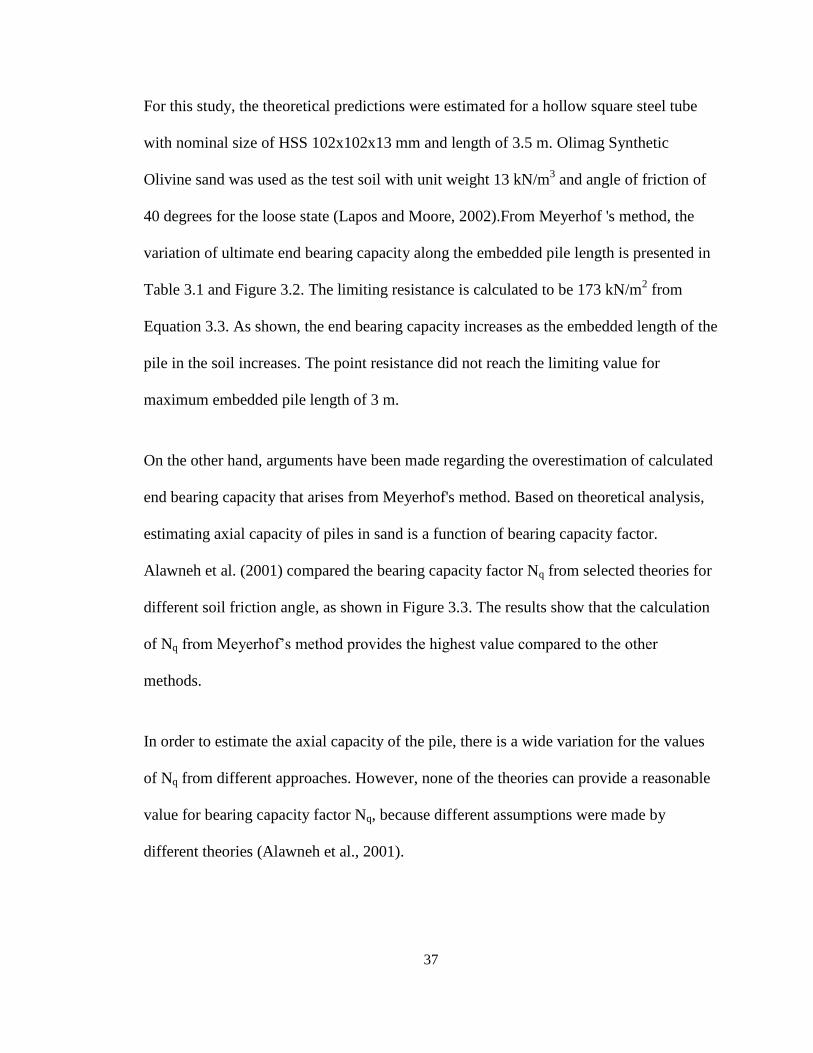
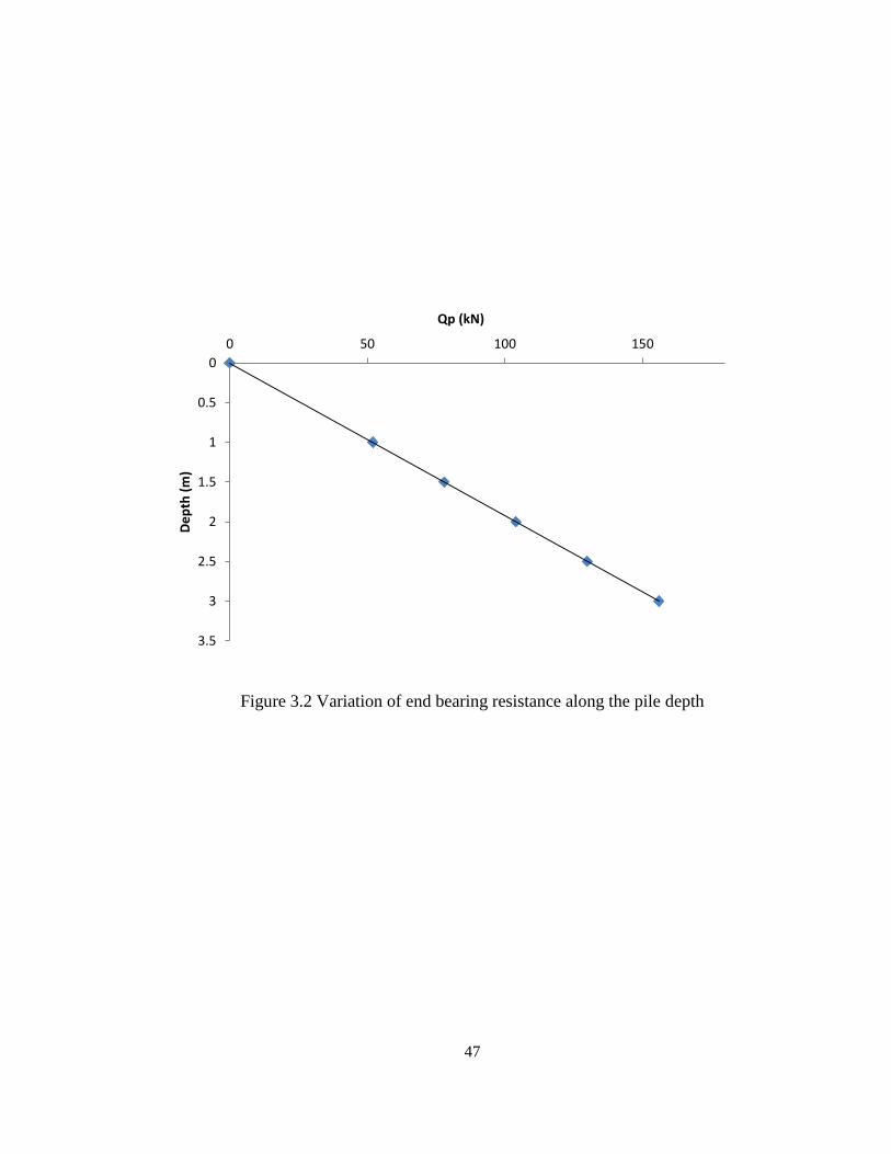
For this study, the theoretical predictions were estimated for a hollow square steel tube
with nominal size of HSS 102x102x13 mm and length of 3.5 m. Olimag Synthetic
Olivine sand was used as the test soil with unit weight 13 kN/m3 and angle of friction of
40 degrees for the loose state (Lapos and Moore, 2002).From Meyerhof 's method, the
variation of ultimate end bearing capacity along the embedded pile length is presented in
Table 3.1 and Figure 3.2. The limiting resistance is calculated to be 173 kN/m2 from
Equation 3.3. As shown, the end bearing capacity increases as the embedded length of the
pile in the soil increases. The point resistance did not reach the limiting value for
maximum embedded pile length of 3 m.
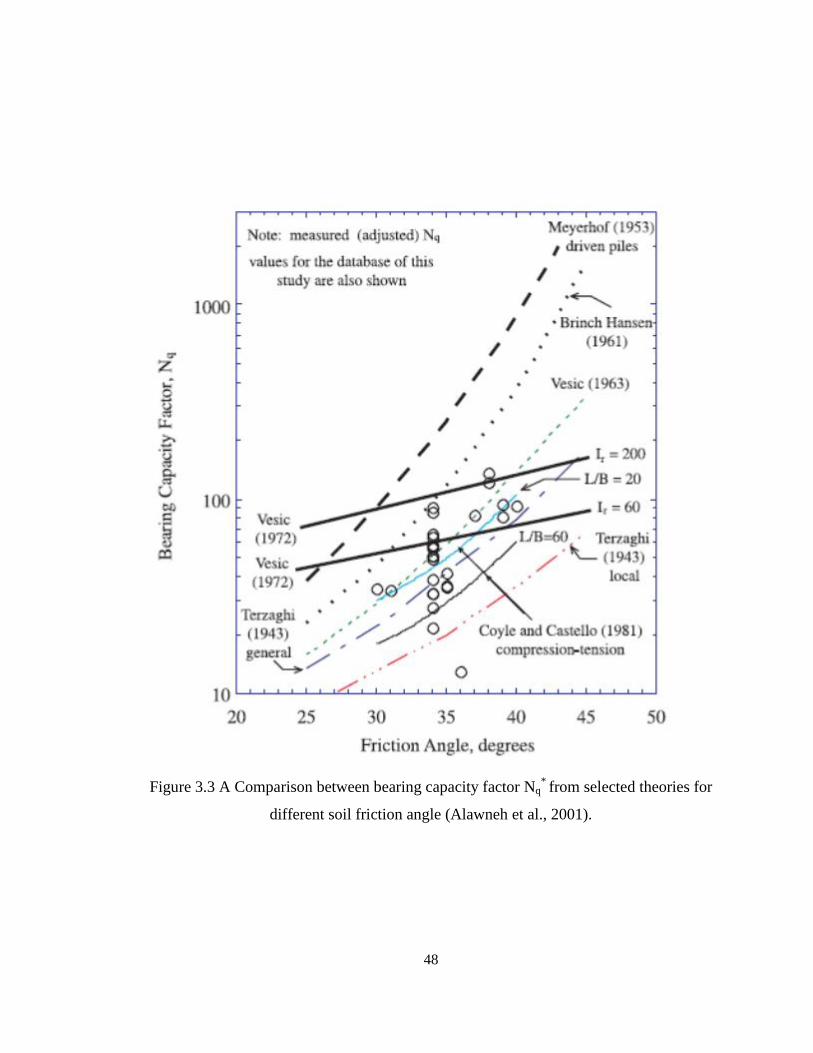
On the other hand, arguments have been made regarding the overestimation of calculated
end bearing capacity that arises from Meyerhof's method. Based on theoretical analysis,
estimating axial capacity of piles in sand is a function of bearing capacity factor.
Alawneh et al. (2001) compared the bearing capacity factor Nq from selected theories for
different soil friction angle, as shown in Figure 3.3. The results show that the calculation
of Nq from Meyerhof’s method provides the highest value compared to the other
methods.
In order to estimate the axial capacity of the pile, there is a wide variation for the values
of Nq from different approaches. However, none of the theories can provide a reasonable
value for bearing capacity factor Nq, because different assumptions were made by
different theories (Alawneh et al., 2001).
38
3.2.2 Shaft Resistance, Qs
Shaft resistance Qs is derived from the shear stresses that develop along the soil-pile
interface. According to Vesic (1970), the shaft resistance is expressed as follows:
Qs= p∑(∆L*fs) [3.4]
where p is the pile perimeter (0.41 m), fs is unit friction resistance and ∆L is incremental
pile length over which fs is constant. The unit friction resistance of a pile increases with
depth linearly only up to a certain depth, called critical depth L. The magnitude of critical
depth is estimated to be 15 to 20 pile diameters. The following equation is used to
calculate the unit friction resistance:
fs = K σoʹ * (tanδ') [3.5]
where K is the effective earth pressure coefficient, σoʹ is the effective vertical stress and δ'
is the soil-pile friction angle. Das (2007) recommended the magnitude of δ' to be (0.6ϕ
')
and K for displacement piles to be 1.4(1- sinϕ').
The critical depth of the test pile is estimated to be 1.9 m with effective earth pressure
coefficient of 0.5 and soil-pile friction angle of 24.6 degrees. The bearing capacity factor
Nq* and the effective earth pressure coefficient K for the theoretical calculation of shaft
resistance are functions of the soil friction angle only. However, the two components, Nq*
and K, are affected by the pile size which is ignored in these calculations (Vesic, 1970).
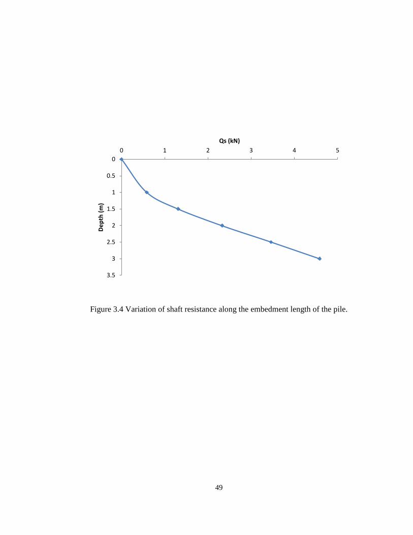
Table 3.2 and Figure 3.4 show the shaft resistance distribution along the embedment
length of the pile. As shown, the shaft resistance increases with the increase in embedded
39
pile length. However, the resistance is concentrated more at the pile toe. As Vesic (1970)
noted, the skin friction is concentrated more at the pile toe for the case of long piles and
along the upper portion for shorter piles (refer to Figure 3.4).
3.2.3 Ultimate Bearing Capacity, Qu
From the calculated end bearing, shaft resistance, weight of the displaced soil and the
weight of the pile, the ultimate axial pile capacity is calculated using Equation 3.1. The
results of axial load capacity are illustrated in Table 3.3 and Figure 3.5. The ultimate
bearing capacity increases linearly as the embedded length of the pile increases. As
mentioned in the previous section, most of the resistance is due to the end bearing
resistance from the pile toe.
3.3 LATERAL CAPACITY
3.3.1 Ultimate Lateral Resistance
Structures on pile foundations may be subjected to lateral forces and movements as a
result of ship impact and wave action in harbour and offshore structures, retaining walls,
high wind forces in transmission-tower foundations, and lateral accelerations acting on
structures in earthquake zones. Therefore, one key issue for pile design may be
estimation of the ultimate lateral resistance. Various methods have been proposed to
estimate the ultimate lateral load capacity Hu (Hansen, 1961; Broms,1964; Petrasovits
and Award, 1972; Prasad and Chari, 1999 and Zhang et a1., 2005). One of the most
popular methods for estimating Hu is Broms' method (Lee et al., 2010). For unrestrained
or free-headed piles, Broms (1964) assumed that the ultimate soil resistance is equal to
40
three times the passive Rankine earth pressure (Poulos and Davis, 1980). The ultimate
lateral resistance is calculated using the following equation:
[3.6]
where Hu is ultimate lateral resistance, γ is unit weight of the soil, d is width or diameter
of the pile, L is embedded length of the pile, e is eccentricity from ground surface to
applied load, and Kp is coefficient of passive earth pressure as calculated by the Rankine
earth pressure theory.
The coefficient Kp can be calculated as:
Kp= tan2(45+
) [3.7]
From the ultimate lateral resistance, the moment is calculated, as shown below.
Mmax= Hu (e+
) [3.8]
The maximum moment occurs at a distance f below the surface. f is function of the soil
and pile properties and the ultimate lateral resistance using the equation:
√
[3.9]
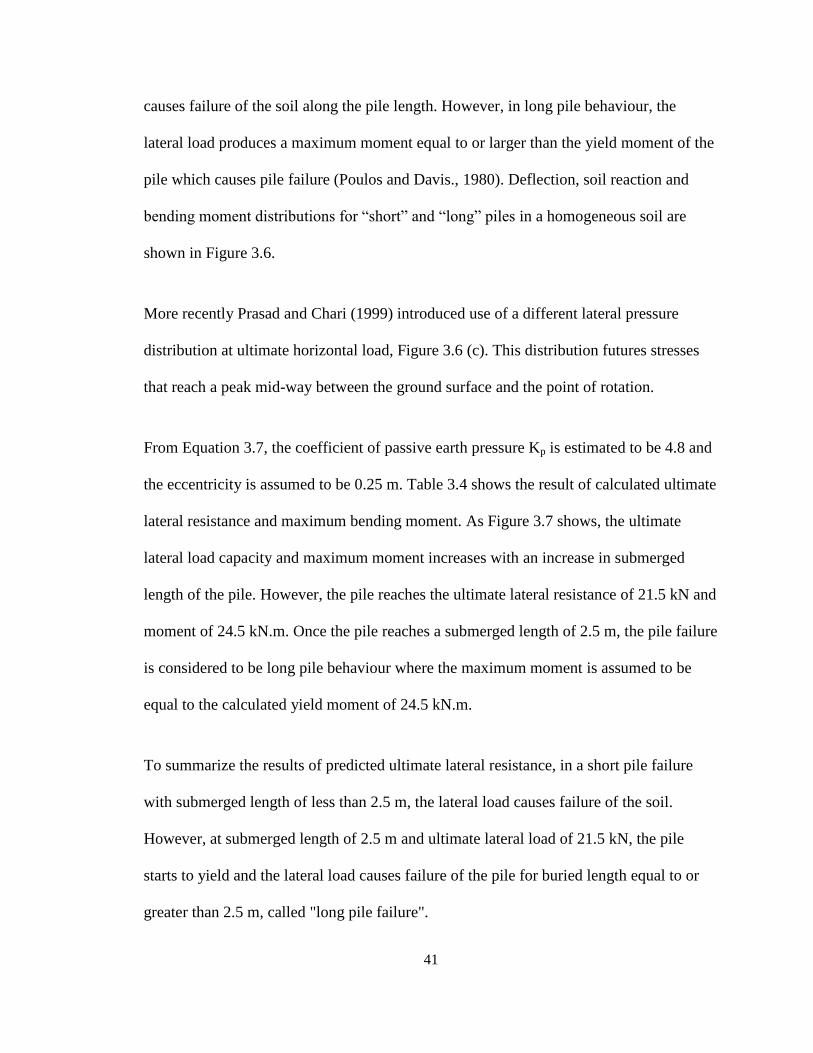
According to Broms (1964), there are two possible failure modes for unrestrained piles in
a cohesionless soil: short and long pile behaviour. In short pile behaviour, the lateral load
41
causes failure of the soil along the pile length. However, in long pile behaviour, the
lateral load produces a maximum moment equal to or larger than the yield moment of the
pile which causes pile failure (Poulos and Davis., 1980). Deflection, soil reaction and
bending moment distributions for “short” and “long” piles in a homogeneous soil are
shown in Figure 3.6.
More recently Prasad and Chari (1999) introduced use of a different lateral pressure
distribution at ultimate horizontal load, Figure 3.6 (c). This distribution futures stresses
that reach a peak mid-way between the ground surface and the point of rotation.
From Equation 3.7, the coefficient of passive earth pressure Kp is estimated to be 4.8 and
the eccentricity is assumed to be 0.25 m. Table 3.4 shows the result of calculated ultimate
lateral resistance and maximum bending moment. As Figure 3.7 shows, the ultimate
lateral load capacity and maximum moment increases with an increase in submerged
length of the pile. However, the pile reaches the ultimate lateral resistance of 21.5 kN and
moment of 24.5 kN.m. Once the pile reaches a submerged length of 2.5 m, the pile failure
is considered to be long pile behaviour where the maximum moment is assumed to be
equal to the calculated yield moment of 24.5 kN.m.
To summarize the results of predicted ultimate lateral resistance, in a short pile failure
with submerged length of less than 2.5 m, the lateral load causes failure of the soil.
However, at submerged length of 2.5 m and ultimate lateral load of 21.5 kN, the pile
starts to yield and the lateral load causes failure of the pile for buried length equal to or
greater than 2.5 m, called "long pile failure".
42
3.4 SUMMARY
Theoretical approaches are used to evaluate axial and lateral capacities of the free-
headed test pile in this chapter. The axial load capacity of a displacement pile is derived
from the sum of the point resistance (Qp) and shaft resistance (Qs). The results show that
the ultimate bearing capacity increases linearly as the embedded length of the pile
increases, with most of the resistance resulting from the pile toe. Axial capacity estimates
were used to design the pile installation system examined in the Chapter 3.
The ultimate lateral resistance of the pile was estimated using Broms' method (1964).
Broms (1964) introduced two possible failure modes for unrestrained piles in a
cohesionless soil: short and long pile behaviour. The result for predicted ultimate lateral
resistance indicates that in a short pile failure with submerged length of less than 2.5 m,
the lateral load causes failure of the soil. However, at submerged length of 2.5 m and
ultimate lateral resistance of 21.5 kN, the pile starts to yield and the lateral load causes
failure of the pile, called "long pile failure". To ensure the test pile was not damaged
during the experiments, a maximum embedded length of 2 m was employed in the
experiments reported in subsequent chapters.
3.5 REFERENCES
Alawneh, A.S., Nusier, O., Husein Malkawi, A.I., and Al-Kateeb, M., 2001, Axial
Compressive Capacity of Driven Piles in Sand: a Method including Post-Driving
Residual Stresses. Canadian Geotechnical Journal, Vol. 38, No. 2, pp. 364-376.
43
Bowles, J.E., 1996, Foundation Analysis and Design. 5th ed. New York: McGraw-Hill
Book Company Inc.
Das, B.M., 2007, Principles of Foundation Engineering. Sixth Edition, Thomson Canada
Limited, pp. 310-319.
Iskander, M., 2010, Behavior of Pipe Piles in Sand. Polytechnic Institute of New York
University, Brooklyn, NY, pp. 75.
Lapos, B. and Moore, I.D, 2002, Evaluation of the strength and deformation parameters
of Olimag synthetic olivine. Proc. of Annual Conference, Canadian Geotechnical
Society, Niagara Falls, ON.
Lee, J., Kim, M., and Kyung, d., 2010, Estimation of Lateral Load Capacity of rigid Short
Piles in Sands Using CPT Results. Journal of Geotechnical and Geoenvironmental
Engineering, Vol. 136, No. 1, pp. 48-56.
Leland, M. and Kraft, Jr., 1991, Performance of Axially Loaded Pipe Piles in Sand.
Journal of Geotechnical Engineering, Vol. 117, No. 2, pp. 272-296.
McGrath, T. J., et al., 2002, NCHRP Report 473: Recommended Specifications for
Large-Span Culverts, Transportation Research Board, National Research Council,
Washington, DC,pp. 6.
Poulos, H.G. and Davis, E.H., 1980, Pile Foundation Analysis and Design. John Wiley &
Sons Inc., pp. 146-152 and pp. 182-185.
44
Veiskarami, M., Eslami, A., and Kumar, j., 2011, End Bearing capacity of Piles in
Sand Using the Stress Characteristics Method: Analysis and Implementation.
Canadian Geotechnical Journal, Vol. 48, No. 10, pp. 1570-1586.
Vesic, A.S., 1970, Tests on Instrumented Piles. Journal of the Soil Mechanics and
Foundations Division, Proceedings of the American Society of Civil engineers.
Vol. 96, No.SM2, pp. 561-583.

45
Table 3.1 Ultimate end bearing capacity along the embedded pile length
Table 3.2 Shaft resistance along the embedment length of the pile.
K 0.5
δ (degrees) 24.6
Embeded length (m) 3 2.5 2 1.5 1 0
Qs (kN) 4.6 3.5 2.4 1.3 0.6 0
Table 3.3 Ultimate bearing capacity.
Embeded length (m) 3 2.5 2 1.5 1 0
Qu (kN) 160 133 105.5 78.5 52 0
Table 3.4 Theoretical ultimate lateral resistance and bending moment.
L (m) 0 0.5 0.75 1.0 1.25 1.50 1.75 2.0 2.25 2.50 2.75 3.0
Hu (kN) 0 0.7 1.70 3.2 5.2 9.0 10.7 15.5 18.3 21.5 21.5 21.5
Mmax (kN.m) 0 0.3 0.9 1.9 3.6 6.0 9.5 14.0 19.6 24.4 24.4 24.4
Ap (m2) 0.01
Nq* 400
ϒ (kN/m3) 13
Embeded length (m) 3 2.5 2 1.5 1 0
Qp (kN) 156 130 104 78 52 0
46
Figure 3.1 Variation of Nq* with soil friction angle ϕ’ (After Meyehof, 1976).
47
Figure 3.2 Variation of end bearing resistance along the pile depth
0
0.5
1
1.5
2
2.5
3
3.5
0 50 100 150
De
pth
(m
)
Qp (kN)
48
Figure 3.3 A Comparison between bearing capacity factor Nq* from selected theories for
different soil friction angle (Alawneh et al., 2001).
49
Figure 3.4 Variation of shaft resistance along the embedment length of the pile.
0
0.5
1
1.5
2
2.5
3
3.5
0 1 2 3 4 5
De
pth
(m
)
Qs (kN)
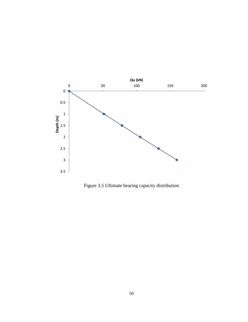
50
Figure 3.5 Ultimate bearing capacity distribution
0
0.5
1
1.5
2
2.5
3
3.5
0 50 100 150 200
De
pth
(m
)
Qu (kN)
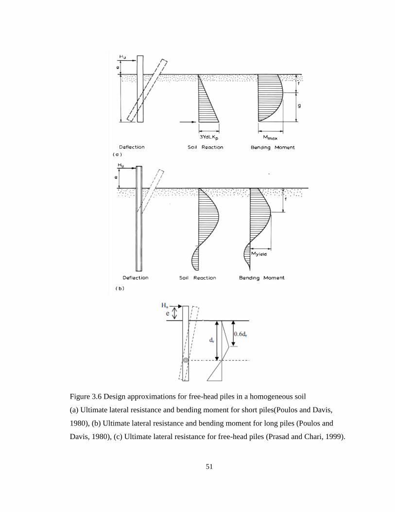
51
Figure 3.6 Design approximations for free-head piles in a homogeneous soil
(a) Ultimate lateral resistance and bending moment for short piles(Poulos and Davis,
1980), (b) Ultimate lateral resistance and bending moment for long piles (Poulos and
Davis, 1980), (c) Ultimate lateral resistance for free-head piles (Prasad and Chari, 1999).
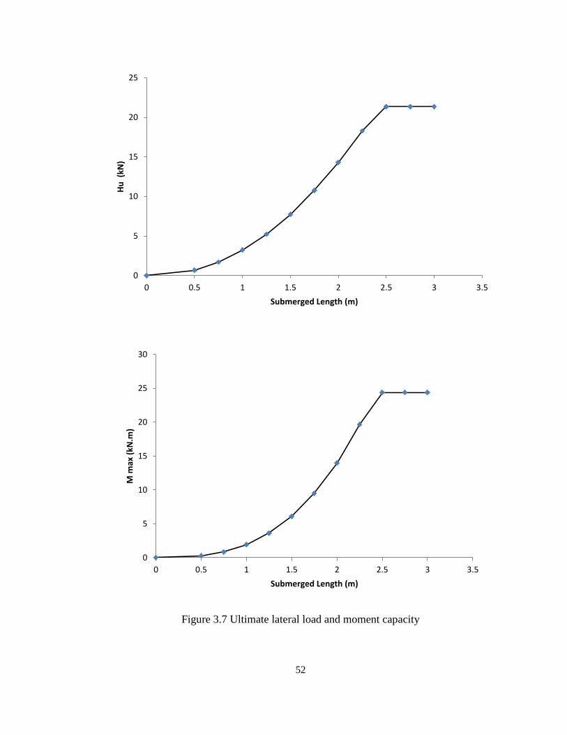
52
Figure 3.7 Ultimate lateral load and moment capacity
0
5
10
15
20
25
0 0.5 1 1.5 2 2.5 3 3.5
Hu
(kN
)
Submerged Length (m)
0
5
10
15
20
25
30
0 0.5 1 1.5 2 2.5 3 3.5
M m
ax (
kN.m
)
Submerged Length (m)
53
Chapter 4
STATIC PILE LOAD TESTS
4.1 INTRODUCTION
Many structures are supported by deep foundations which must be designed to resist axial
and lateral loadings (Caliendo and Anderson, 1996). Therefore, pile load tests may be
conducted in the design phase or at the start of construction to demonstrate the suitability
of the pile foundation system. Many research studies have been conducted to understand
pile behaviour under axial and lateral loading using theoretical approaches. Although
these are valuable means for investigating pile behaviour and undertaking foundation
design, they require evaluation against measurements so their performance can be
assessed and improvements made to produce even better design models.
As Poulos and Davis (1980) noted, Broms theory is based on a number of assumptions
for ultimate lateral load analysis:
a. The active earth pressure is neglected;
b. The passive pressure is equal to three times the Rankine passive pressure;
c. The distribution of ultimate lateral resistance is not a function of the pile shape;
d. The movements are sufficient to mobilize the full lateral resistance
In addition, Poulos and Davis (1980) indicate that laterally loaded pile analysis using the
theoretical methods is based on a constant structural stiffness. In general, an increase in
the lateral load prior to failure may cause cracks to form in the pile which leads to a
reduction in the structural stiffness of the pile (Ismael, 2010). However, the current study
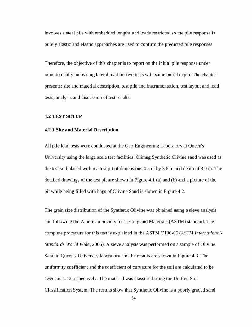
54
involves a steel pile with embedded lengths and loads restricted so the pile response is
purely elastic and elastic approaches are used to confirm the predicted pile responses.
Therefore, the objective of this chapter is to report on the initial pile response under
monotonically increasing lateral load for two tests with same burial depth. The chapter
presents: site and material description, test pile and instrumentation, test layout and load
tests, analysis and discussion of test results.
4.2 TEST SETUP
4.2.1 Site and Material Description
All pile load tests were conducted at the Geo-Engineering Laboratory at Queen's
University using the large scale test facilities. Olimag Synthetic Olivine sand was used as
the test soil placed within a test pit of dimensions 4.5 m by 3.6 m and depth of 3.0 m. The
detailed drawings of the test pit are shown in Figure 4.1 (a) and (b) and a picture of the
pit while being filled with bags of Olivine Sand is shown in Figure 4.2.
The grain size distribution of the Synthetic Olivine was obtained using a sieve analysis
and following the American Society for Testing and Materials (ASTM) standard. The
complete procedure for this test is explained in the ASTM C136-06 (ASTM International-
Standards World Wide, 2006). A sieve analysis was performed on a sample of Olivine
Sand in Queen's University laboratory and the results are shown in Figure 4.3. The
uniformity coefficient and the coefficient of curvature for the soil are calculated to be
1.65 and 1.12 respectively. The material was classified using the Unified Soil
Classification System. The results show that Synthetic Olivine is a poorly graded sand
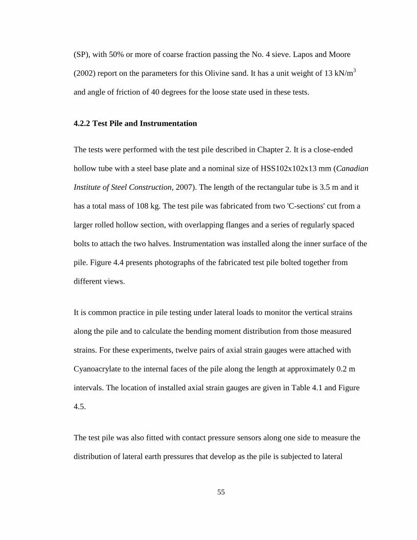
55
(SP), with 50% or more of coarse fraction passing the No. 4 sieve. Lapos and Moore
(2002) report on the parameters for this Olivine sand. It has a unit weight of 13 kN/m3
and angle of friction of 40 degrees for the loose state used in these tests.
4.2.2 Test Pile and Instrumentation
The tests were performed with the test pile described in Chapter 2. It is a close-ended
hollow tube with a steel base plate and a nominal size of HSS102x102x13 mm (Canadian
Institute of Steel Construction, 2007). The length of the rectangular tube is 3.5 m and it
has a total mass of 108 kg. The test pile was fabricated from two 'C-sections' cut from a
larger rolled hollow section, with overlapping flanges and a series of regularly spaced
bolts to attach the two halves. Instrumentation was installed along the inner surface of the
pile. Figure 4.4 presents photographs of the fabricated test pile bolted together from
different views.
It is common practice in pile testing under lateral loads to monitor the vertical strains
along the pile and to calculate the bending moment distribution from those measured
strains. For these experiments, twelve pairs of axial strain gauges were attached with
Cyanoacrylate to the internal faces of the pile along the length at approximately 0.2 m
intervals. The location of installed axial strain gauges are given in Table 4.1 and Figure
4.5.
The test pile was also fitted with contact pressure sensors along one side to measure the
distribution of lateral earth pressures that develop as the pile is subjected to lateral
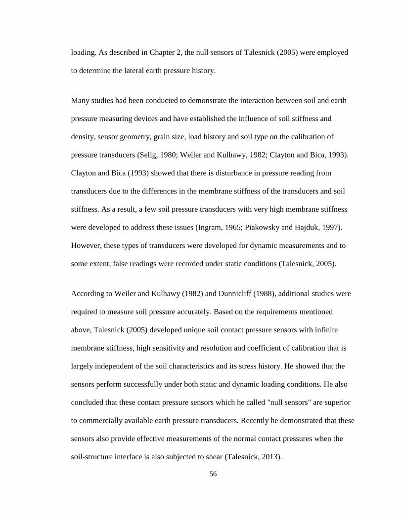
56
loading. As described in Chapter 2, the null sensors of Talesnick (2005) were employed
to determine the lateral earth pressure history.
Many studies had been conducted to demonstrate the interaction between soil and earth
pressure measuring devices and have established the influence of soil stiffness and
density, sensor geometry, grain size, load history and soil type on the calibration of
pressure transducers (Selig, 1980; Weiler and Kulhawy, 1982; Clayton and Bica, 1993).
Clayton and Bica (1993) showed that there is disturbance in pressure reading from
transducers due to the differences in the membrane stiffness of the transducers and soil
stiffness. As a result, a few soil pressure transducers with very high membrane stiffness
were developed to address these issues (Ingram, 1965; Piakowsky and Hajduk, 1997).
However, these types of transducers were developed for dynamic measurements and to
some extent, false readings were recorded under static conditions (Talesnick, 2005).
According to Weiler and Kulhawy (1982) and Dunnicliff (1988), additional studies were
required to measure soil pressure accurately. Based on the requirements mentioned
above, Talesnick (2005) developed unique soil contact pressure sensors with infinite
membrane stiffness, high sensitivity and resolution and coefficient of calibration that is
largely independent of the soil characteristics and its stress history. He showed that the
sensors perform successfully under both static and dynamic loading conditions. He also
concluded that these contact pressure sensors which he called "null sensors" are superior
to commercially available earth pressure transducers. Recently he demonstrated that these
sensors also provide effective measurements of the normal contact pressures when the
soil-structure interface is also subjected to shear (Talesnick, 2013).
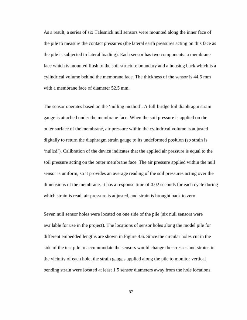
57
As a result, a series of six Talesnick null sensors were mounted along the inner face of
the pile to measure the contact pressures (the lateral earth pressures acting on this face as
the pile is subjected to lateral loading). Each sensor has two components: a membrane
face which is mounted flush to the soil-structure boundary and a housing back which is a
cylindrical volume behind the membrane face. The thickness of the sensor is 44.5 mm
with a membrane face of diameter 52.5 mm.
The sensor operates based on the ‘nulling method’. A full-bridge foil diaphragm strain
gauge is attached under the membrane face. When the soil pressure is applied on the
outer surface of the membrane, air pressure within the cylindrical volume is adjusted
digitally to return the diaphragm strain gauge to its undeformed position (so strain is
‘nulled’). Calibration of the device indicates that the applied air pressure is equal to the
soil pressure acting on the outer membrane face. The air pressure applied within the null
sensor is uniform, so it provides an average reading of the soil pressures acting over the
dimensions of the membrane. It has a response time of 0.02 seconds for each cycle during
which strain is read, air pressure is adjusted, and strain is brought back to zero.
Seven null sensor holes were located on one side of the pile (six null sensors were
available for use in the project). The locations of sensor holes along the model pile for
different embedded lengths are shown in Figure 4.6. Since the circular holes cut in the
side of the test pile to accommodate the sensors would change the stresses and strains in
the vicinity of each hole, the strain gauges applied along the pile to monitor vertical
bending strain were located at least 1.5 sensor diameters away from the hole locations.
58
To prevent the sensors being pushed into the hollow pile and maintain zero pressure
readings during bending, the null sensors were held in place using steel brackets bolted to
the pile above the null sensor. Each bracket was 76 mm long with square cross section of
20 mm x 20 mm. Two screws, with nominal size M 5x2, extend from the bracket so that
they touch the rear surface of the null sensor and hold it in position. The brackets are not
screwed to the sensors so that strains do not develop in the sensors as a result of
longitudinal bending strains induced in the pile as it is subjected to lateral loading.
Horizontal deflections of the pile were measured using string potentiometers (‘string
pots’). String pots were installed at two different vertical positions: at the point where
lateral loading was applied and 0.50 m above the loading point. These two measurements
then permit the deformations of the pile (lateral displacement) to be calculated by
assuming it responds as a rigid body. Figure 4.7 shows the string pots attached before
commencing one of the lateral loading tests.
4.2.3 Limitation for Test Layout
The large scale pile load tests were conducted in a test pit located at the Geo-Engineering
Laboratory at Queen's University. One set of loose test soil was prepared for all of the
five tests reported in Chapters 4 and 5, so as to reduce testing costs (associated with
removal and replacement of the test sand from the pit) and testing time, while having all
results generated in soil of the same density (though some variation in initial soil density
can be expected across the test pit because no soil placement process is perfectly uniform,
it avoids changes in density that might occur between placement events as a result of
inadvertent changes in soil moisture or placement technique). Furthermore, each location
59
used for the test pile within the pit was chosen to minimize interaction with the pit
boundaries in front of, behind, and beside the test pile. The choices of test pile location,
however, depend on the size of the zone where changes in soil density occur around each
specific test pile location within the pit, as discussed in the following paragraphs.
Two phases of the testing need to be considered when assessing the proximity of different
test pile locations and distances to the pit boundaries. The first phase is pile insertion,
where the pile is loaded axially, displacing the soil under the end of the pile downwards
and the soil beside it radially from the centreline. The second test stage involves lateral
loading, when the pile translates laterally and rotates as a rigid body within the test sand.
Soil responses during the pile insertion stage are similar to those that occur during cone
penetrometer testing within a cylindrical test chamber. Houlsby and Hitchman (1988)
used a test chamber featuring a radial distance of 12.5 cone diameters from the central
axis to the external chamber boundary. In their subsequent response to discussions of
their paper, they refer to cavity expansion analysis and a review of 400 different cone
penetration tests conducted by various researchers, and conclude that test results
exhibited ‘little chamber size effect’ for experiments conducted in loose sand, but
‘significant effect’ for dense sands.
While no effect of boundary conditions is therefore expected as the test pile is pushed
into the loose sand (Baziar and Moayed, 2006) and no minimum limit is suggested for
loose sand testing, Houlsby and Hitchman (1988) indicate that a distance of 8 diameters
to an external boundary and 4 diameters to a zone of soil influenced by a previous test is
60
sufficient for the pile insertion phase of the experiments, given the loose condition of the
test sand and the fact that the lateral pit dimensions are actually much larger. For the
experiments reported here, minimum distance to external boundary was 0.9 m (over 8
diameters), and minimum distance to another pile test location was 0.6 m (almost 6
diameters).
In addition, the test pile length should be limited to minimize the effect of upper and
lower boundaries. According to Caliendo and Anderson (1996), the base of the pile must
be no closer than three pile diameters to the bottom of the test pit to minimize the effect
of that base boundary. The minimum distance used in the pile tests reported here was 1.0
m (more than three diameters).
The zone of influence around the test pile during the second phase featuring lateral
loading and translation has similarities to the soil-structure interaction that occurs when a
stiff steel pipe is pulled laterally through the soil. Kenny (2013) studied pipes moving
laterally through the ground, and recommended that a leading distance of 7 diameters and
a trailing distance of at least 3 diameters is required to control boundary effects.
Converting the 0.1 m by 0.1 m square test pile cross-section into a circle of the same area,
equivalent diameter is 0.11 m. Proximity guidelines for the pile during installation are
therefore adopted featuring a minimum distance of 0.9 m to a lateral boundary of the test
pit, and half that to the location of another position where the pile was previously
installed and tested. For the lateral loading phase of the test, a minimum distance of 1.0 m
is adopted ahead of the pile, and 0.9 m behind and beside it.
61
4.2.4 Test Layout and Loading Procedure
Two (2) sets of static pile load tests were performed in Olimag Synthetic Olivine sand in
the pit of 4.5 m 3.6 m and depth of 3.0 m. The locations of the model pile in the pit for
two sets of static tests followed the limitation guidelines for test layout and are presented
in Figure 4.8.
In Test 1, the test pile was inserted a distance 2.0 m into the soil at a location 0.9 m to the
North and 1.0 m to the West of the corner of the test pit (see Figure 4.8). Lateral loads
were then applied on pile side A where the null sensors were located. The load was
applied 0.25 m above the ground surface (the distance normally referred to as
eccentricity). The pile was then removed, rotated 180 degrees so pressures could be
monitored on the opposite side, and inserted at the second position. Test 2, again featured
insertion of the pile by 2.0 m, but this time at a location 1.4 m to the North-West from the
corner of the test pit (0.5 m to the North and 0.4 m to the West of the location used for
Test 1, i.e. 0.64 m away). The choice of these two locations left other positions in the
Test pit available for subsequent tests (those reported in Chapter 5).
To insert the pile into the sandy soil, axial loads were applied using a hydraulic jack
mounted between a reaction beam passing over the pit and the end-plate. Figure 4.9
shows a typical load test arrangement which is similar to the loading layout used for this
test program. The reaction beam attached to a fixed reference steel frame was sufficient
to resist a maximum axial capacity of 100 kN. The actuator was connected to a hydraulic
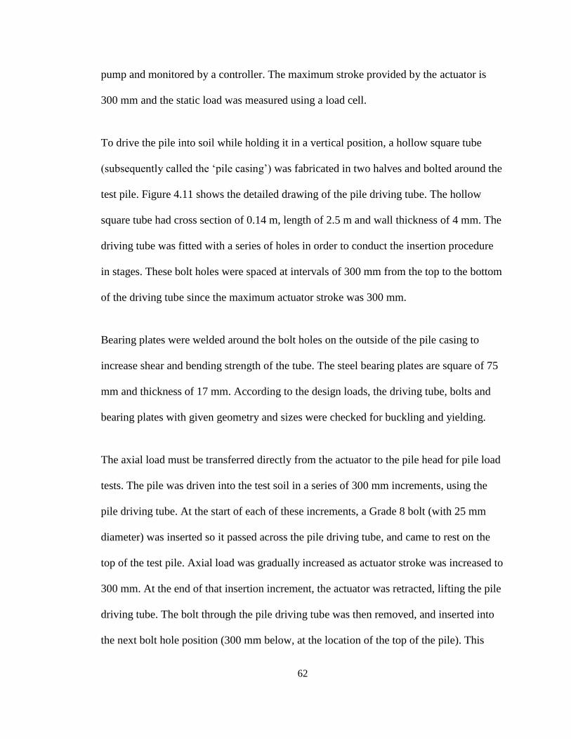
62
pump and monitored by a controller. The maximum stroke provided by the actuator is
300 mm and the static load was measured using a load cell.
To drive the pile into soil while holding it in a vertical position, a hollow square tube
(subsequently called the ‘pile casing’) was fabricated in two halves and bolted around the
test pile. Figure 4.11 shows the detailed drawing of the pile driving tube. The hollow
square tube had cross section of 0.14 m, length of 2.5 m and wall thickness of 4 mm. The
driving tube was fitted with a series of holes in order to conduct the insertion procedure
in stages. These bolt holes were spaced at intervals of 300 mm from the top to the bottom
of the driving tube since the maximum actuator stroke was 300 mm.
Bearing plates were welded around the bolt holes on the outside of the pile casing to
increase shear and bending strength of the tube. The steel bearing plates are square of 75
mm and thickness of 17 mm. According to the design loads, the driving tube, bolts and
bearing plates with given geometry and sizes were checked for buckling and yielding.
The axial load must be transferred directly from the actuator to the pile head for pile load
tests. The pile was driven into the test soil in a series of 300 mm increments, using the
pile driving tube. At the start of each of these increments, a Grade 8 bolt (with 25 mm
diameter) was inserted so it passed across the pile driving tube, and came to rest on the
top of the test pile. Axial load was gradually increased as actuator stroke was increased to
300 mm. At the end of that insertion increment, the actuator was retracted, lifting the pile
driving tube. The bolt through the pile driving tube was then removed, and inserted into
the next bolt hole position (300 mm below, at the location of the top of the pile). This
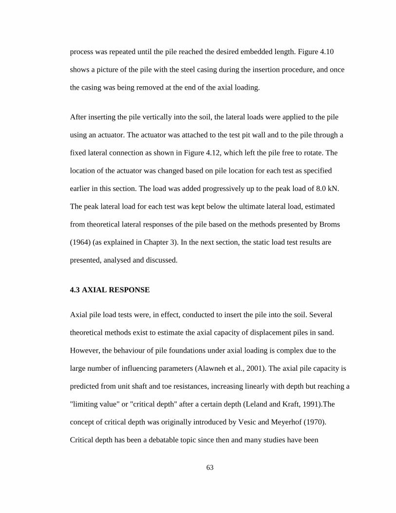
63
process was repeated until the pile reached the desired embedded length. Figure 4.10
shows a picture of the pile with the steel casing during the insertion procedure, and once
the casing was being removed at the end of the axial loading.
After inserting the pile vertically into the soil, the lateral loads were applied to the pile
using an actuator. The actuator was attached to the test pit wall and to the pile through a
fixed lateral connection as shown in Figure 4.12, which left the pile free to rotate. The
location of the actuator was changed based on pile location for each test as specified
earlier in this section. The load was added progressively up to the peak load of 8.0 kN.
The peak lateral load for each test was kept below the ultimate lateral load, estimated
from theoretical lateral responses of the pile based on the methods presented by Broms
(1964) (as explained in Chapter 3). In the next section, the static load test results are
presented, analysed and discussed.
4.3 AXIAL RESPONSE
Axial pile load tests were, in effect, conducted to insert the pile into the soil. Several
theoretical methods exist to estimate the axial capacity of displacement piles in sand.
However, the behaviour of pile foundations under axial loading is complex due to the
large number of influencing parameters (Alawneh et al., 2001). The axial pile capacity is
predicted from unit shaft and toe resistances, increasing linearly with depth but reaching a
"limiting value" or "critical depth" after a certain depth (Leland and Kraft, 1991).The
concept of critical depth was originally introduced by Vesic and Meyerhof (1970).
Critical depth has been a debatable topic since then and many studies have been
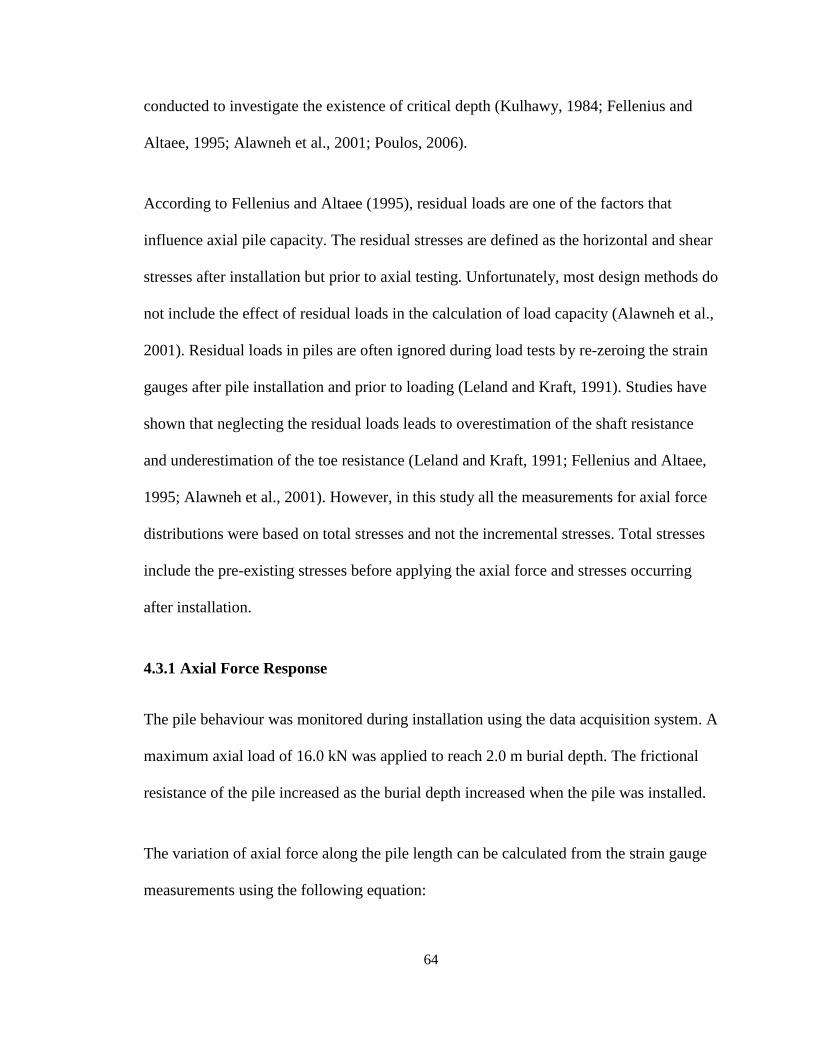
64
conducted to investigate the existence of critical depth (Kulhawy, 1984; Fellenius and
Altaee, 1995; Alawneh et al., 2001; Poulos, 2006).
According to Fellenius and Altaee (1995), residual loads are one of the factors that
influence axial pile capacity. The residual stresses are defined as the horizontal and shear
stresses after installation but prior to axial testing. Unfortunately, most design methods do
not include the effect of residual loads in the calculation of load capacity (Alawneh et al.,
2001). Residual loads in piles are often ignored during load tests by re-zeroing the strain
gauges after pile installation and prior to loading (Leland and Kraft, 1991). Studies have
shown that neglecting the residual loads leads to overestimation of the shaft resistance
and underestimation of the toe resistance (Leland and Kraft, 1991; Fellenius and Altaee,
1995; Alawneh et al., 2001). However, in this study all the measurements for axial force
distributions were based on total stresses and not the incremental stresses. Total stresses
include the pre-existing stresses before applying the axial force and stresses occurring
after installation.
4.3.1 Axial Force Response
The pile behaviour was monitored during installation using the data acquisition system. A
maximum axial load of 16.0 kN was applied to reach 2.0 m burial depth. The frictional
resistance of the pile increased as the burial depth increased when the pile was installed.
The variation of axial force along the pile length can be calculated from the strain gauge
measurements using the following equation:
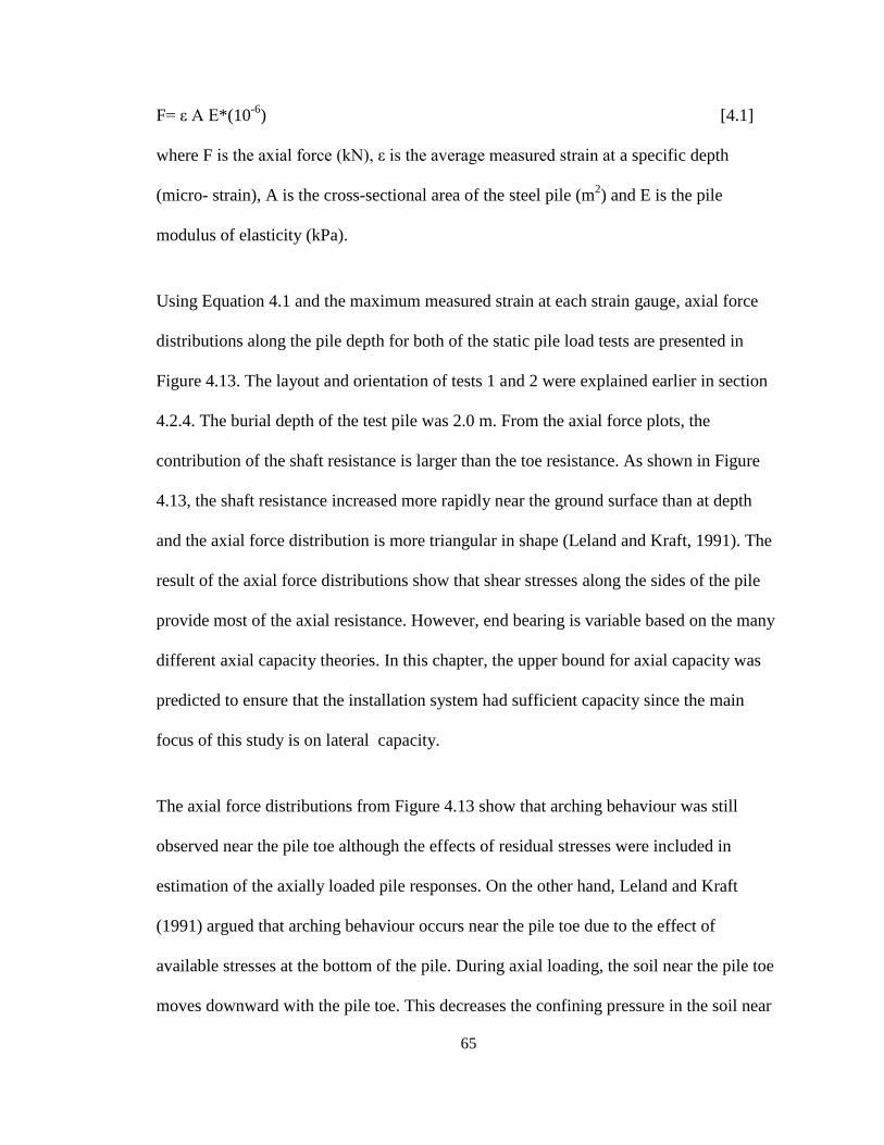
65
F= ε A E*(10-6
) [4.1]
where F is the axial force (kN), ε is the average measured strain at a specific depth
(micro- strain), A is the cross-sectional area of the steel pile (m2) and E is the pile
modulus of elasticity (kPa).
Using Equation 4.1 and the maximum measured strain at each strain gauge, axial force
distributions along the pile depth for both of the static pile load tests are presented in
Figure 4.13. The layout and orientation of tests 1 and 2 were explained earlier in section
4.2.4. The burial depth of the test pile was 2.0 m. From the axial force plots, the
contribution of the shaft resistance is larger than the toe resistance. As shown in Figure
4.13, the shaft resistance increased more rapidly near the ground surface than at depth
and the axial force distribution is more triangular in shape (Leland and Kraft, 1991). The
result of the axial force distributions show that shear stresses along the sides of the pile
provide most of the axial resistance. However, end bearing is variable based on the many
different axial capacity theories. In this chapter, the upper bound for axial capacity was
predicted to ensure that the installation system had sufficient capacity since the main
focus of this study is on lateral capacity.
The axial force distributions from Figure 4.13 show that arching behaviour was still
observed near the pile toe although the effects of residual stresses were included in
estimation of the axially loaded pile responses. On the other hand, Leland and Kraft
(1991) argued that arching behaviour occurs near the pile toe due to the effect of
available stresses at the bottom of the pile. During axial loading, the soil near the pile toe
moves downward with the pile toe. This decreases the confining pressure in the soil near
66
the toe and as a result, the axial force near the toe goes to approximately zero value
(Leland and Kraft, 1991 after Robinsky and Morrison, 1964).
4.3.2 Moment Response
The maximum bending moment distributions were estimated based on measured strains
along the pile length for tests 1 and 2. The results show that moments were developed
during pile installation. No moment would be recorded if it was a perfect installation.
However the pile was not installed perfectly vertical, and small moment was recorded
(refer to Appendix for moment responses).
4.3.3 Earth Pressure Response
Figure 4.14 shows the maximum normal contact pressure distribution along the test pile
at the end of installation to the selected embedded length (2.0 m). The measured
pressures indicate that the horizontal earth pressures ranged between 0 kPa to 8 kPa.
Therefore, the lateral earth pressures on the test pile were low during pile insertion.
4.3.4 Comparison with Existing Design Methods
The primary purpose of this study was to examine lateral capacity of the pile in sand.
However, since some axial measurements were recorded during pile installation, the axial
capacity was explained briefly. The axial load capacity of a pile is computed based on the
unit shaft and toe resistances from the theoretical approaches. As discussed earlier in
Chapter 3, the predicted axial capacity of piles in sand is a function of bearing capacity
factor Nq and this value varies widely between theories.
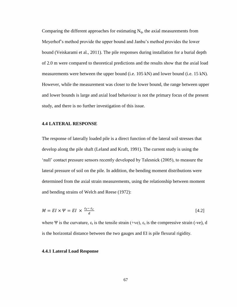
67
Comparing the different approaches for estimating Nq, the axial measurements from
Meyerhof’s method provide the upper bound and Janbu’s method provides the lower
bound (Veiskarami et al., 2011). The pile responses during installation for a burial depth
of 2.0 m were compared to theoretical predictions and the results show that the axial load
measurements were between the upper bound (i.e. 105 kN) and lower bound (i.e. 15 kN).
However, while the measurement was closer to the lower bound, the range between upper
and lower bounds is large and axial load behaviour is not the primary focus of the present
study, and there is no further investigation of this issue.
4.4 LATERAL RESPONSE
The response of laterally loaded pile is a direct function of the lateral soil stresses that
develop along the pile shaft (Leland and Kraft, 1991). The current study is using the
‘null’ contact pressure sensors recently developed by Talesnick (2005), to measure the
lateral pressure of soil on the pile. In addition, the bending moment distributions were
determined from the axial strain measurements, using the relationship between moment
and bending strains of Welch and Reese (1972):
[4.2]
where Ψ is the curvature, εt is the tensile strain (+ve), εc is the compressive strain (-ve), d
is the horizontal distance between the two gauges and EI is pile flexural rigidity.
4.4.1 Lateral Load Response
68
Figure 4.15 presents the graph of applied lateral load over the monitoring period for Tests
1 and 2. The pile burial depth is 2.0 m for both of the tests but the location of pile in the
test pit is different. Brom's theoretical method shows that the ultimate lateral resistance is
estimated to be 15.5 kN for burial depth of 2.0 m (see Chapter 3). A maximum applied
lateral load of 8.0 kN was applied over the monitoring period to avoid pile yielding.
In each test, the pile was loaded laterally until the maximum load of 8.0 kN was reached.
The maximum load was held for approximately six minutes and the pile was unloaded to
lateral load of 1 kN. In the next sections, the pile response under lateral loading will be
discussed.
4.4.2 Bending Moment Response
Using Equation 4.2, the bending moment distributions are estimated from the maximum
measured strain and flexural rigidity of 1015 kN.m2 obtained from the bending test as
discussed in detail in Chapter 2. The bending moment responses calculated for laterally
loaded pile Tests 1 and 2 are presented in Figure 4.16.
As shown in the bending moment plots, the moment distributions follow the same
pattern and the location of maximum moment for both of the tests are in good agreement.
The results show that maximum moments of 5.6 and 5.4 kN.m (mean 5.5 kN.m) for Tests
1 and 2, respectively at a position approximately 1.3 m above the pile toe were observed
for Tests 1 and 2. These results indicate that the soil and other test conditions are almost
the same in the two tests. They provide strong support for the consistency of the pile
insertion process, and the density, stiffness and strength of the soil around the pile during
69
the two experiments, and that any differences have little influence on the moment
distributions that arise for a specific level of applied horizontal force.
4.4.3 Load-Deflection Response
While Figure 4.16 indicates that the bending moment distributions associated with a
specific level of horizontal force were very similar for Tests 1 and 2, a comparison of the
load-deflection responses is now made to examine whether the stiffness of the soil
support provided to the pile during the two tests was also consistent. In addition, load-
deflection plots can be monitored to confirm that the pile is not loaded beyond the elastic
limit or yield point (Matsumoto et al., 2001). Figure 4.17 illustrates the recorded load
versus the deflection at the loading point for Tests 1 and 2. As the load increases, the
slope of load-deflection curve decreases due to a decrease in the stiffness of soil (Rollins
et al., 2005). As shown in the figure, the pile was not loaded beyond its ultimate lateral
capacity and the magnitude of the strain measurements indicate that the pile responses are
within the elastic range (though the soil response is nonlinear).
For the case of linear elastic behaviour, the buried pile stiffness is calculated from the
slope of load-deflection diagram. The horizontal pile movements for both tests were
similar since the burial depth and loading conditions were almost identical. However, a
maximum discrepancy in the displacement of about 3.0 mm occurred at the maximum
lateral load for Tests 1 and 2. Many factors may influence the load-deflection response of
the test pile under static lateral loading. Although boundary conditions have a significant
effect on lateral response of a pile in dense soil, there is little effect in loose soil (Houlsby
and Hitmach, 1988; Baziar and Moayed, 2006).
70
Giannakos et al. (2012) performed experiments on lateral response of a pile in a dry sand
and have shown that the loading rate has a significant effect on the pile response. In
addition, the soil is displaced and disturbed as the pile deflects during the previous tests.
This difference in soil stiffness may mean that the sand in test 2 was not quite the same as
it was in the first test, perhaps as a result of changes in soil density during Test 1. It might
be a reflection of initial soil density (before Test 1) that was not uniform across the test
pit. Also, there is always the potential for human errors and instrument inaccuracy. The
difference in maximum soil displacement at the same horizontal force was approximately
10%. Subsequent comparisons in behaviour during the two tests are largely confined to
evaluations of stresses and stress resultants, which were seen in the previous section to be
largely immune to changes in soil density or other test characteristics (provided they are
made at the same level of applied force, rather than the same level of lateral translation
and/or rotation of the pile).
4.4.4 Earth Pressure Response
Perhaps the most important objectives of this study of laterally loaded piles are associated
with the measurement of lateral (horizontal) earth pressures along the pile depth using the
null sensors. The pressure distributions along the pile burial depth for Tests 1 and 2 are
plotted in Figure 4.18. As mentioned in section 4.2.4 (Test Layout and Loading
Procedure), the lateral load was applied on pile side A, where the null sensors are located
in test 1 and on pile side B in test 2. In order to present the pressure distribution plots for
both tests on the same graph, negative values denote the pressure readings when the load
is pushing in the same direction as the stresses acting on the null sensors, and positive
71
values denoted the reverse (where the pressure on the sensors is in the direction opposite
to that of the applied load).
For the maximum horizontal applied load of 8.0 kN over the monitoring period used
during Tests 1 and 2, the pressure values are in the range of -140.0 kPa to 160.0 kPa. The
pressure distributions show that the maximum pressure of -140.0 kPa was observed just
above the toe when pile rotation leads to the null sensor moving in the direction opposite
to that of the applied load. Significant lateral stresses were recorded on the sensors when
they are being pushed into the soil. However, almost zero stresses were recorded when
the sensors were moving away from the soil. In both tests, pressures of almost zero were
recorded at a height of 0.6 m above the bottom of the pile. Therefore, the point of rotation
of the pile is interpreted to be at that position (0.6 m above the toe).
A lateral force distribution per unit length (i.e. height) for these static lateral pile load
tests has been presented in Figure 4.19 (denoted as the curve marked 'uniform'), where
this lateral force distribution was calculated from the contact pressure measurements
assuming that the lateral pressures are uniformly distributed across the whole of the 0.1 m
wide pile, that zero shear stress develops on the sides of the test pile, and that stresses at
the back (where the sensors are moving away from the soil) are zero.
From Figure 4.19, the calculated values of lateral force can be integrated up the pile to
determine whether they equal the total applied horizontal force. Approximating the
distribution as triangular in shape, the total calculated force is 7.5 kN. This is 94% of the
load of 8 kN applied by the actuator. Use of a nonlinear polynomial to approximate the
72
earth pressures distribution on the pile might produce an estimate of total horizontal force
that is even closer to 8kN.
Several theoretical methods have been established to predict the behaviour of short rigid
piles under lateral loading in cohesionless soil (Brinch Hansen, 1961; Broms, 1964;
Petrasovits and Award, 1972, Meyerhof et al., 1987). However, Prasad and Chari (1999)
found that available theoretical predictions of the ultimate lateral capacity are based on
simplified earth pressure distributions which are different from the actual soil pressure
distribution along the pile length. According to Prasad and Chari (1999), the variation of
peak pressure distribution for a rigid pile under monotonic loading can be idealized as a
linear increase up to distance 0.6 times the depth of rotation point. Then, the pressure
decreases to zero at the point of rotation and increases in the other direction to maximum
at the pile toe, see Figure 3.6 (c).
The lateral pressure results from Tests 1 and 2 (see Figure 4.18) show that the
distributions follow the same pattern of pressures presented by Prasad and Chari (1999).
However, the pressure distributions cannot be numerically compared with that existing
design method of Prasad ad Chari (1999) since the lateral peak load in Tests 1 and 2 did
not reach the ultimate capacity, while Prasad and Chari predicted the variation of pressure
distributions at the peak state along the length of the pile. Future analysis on peak lateral
pressures under monotonic loading is recommended to compare the results with existing
design methods by Prasad and Chari (1999).
73
4.4.5 Measuring Lateral Pressure and Deflection from Moment Distribution
Moment Distribution
The moment distribution can be calculated from statics using moment equilibrium,
considering the maximum applied lateral load and the lateral pressure distribution
obtained from the null sensors. The results are compared to the moment distribution
interpreted from the strains (curvatures) measured during the static lateral load tests as
shown in Figure 4.20. The moment distributions calculated from measured pressures and
curvatures have the same pattern, but with moments from pressures falling below those
from curvatures up to a point 1.4 m above the pile toe.
As mentioned earlier, the moment from statics is calculated from the horizontal pressure
obtained from the null sensors. This calculation implicitly assumes that all the recorded
pressures from the null sensors are precise, that these pressures are uniformly distributed
across the whole pile width, and that no horizontal shear stresses develop on the sides of
the pile perpendicular to the face with the pressure sensors. However, the comparison of
applied horizontal force to summation of horizontal earth pressures from the sensors
examined in the previous section (Figure 4.19) already revealed that these assumptions
are questionable. Horizontal shear stress may also develop at the bottom the pile, which
would also influence the horizontal force resultant and the distribution of bending
moment. The discrepancy between moment from curvature and from measured pressures
is 1.0 kN.m at height of 0.6 m above the toe and 0.34 kN.m at height of 0.2 m above the
toe. These discrepancies suggest that a shear force is acting at the bottom of the pile. If
that force has magnitude of 1.7 kN, it would resolve most of the discrepancy between
74
moment values at heights of 0.2 m and 0.6 m, though it would also lead to changes above
that position and it would influence the calculation of horizontal force resultant examined
in the previous section. In the future, measurement of the base pressure using a stress
sensor located in the base plate would assist in the interpretation of pressures and
moments, since it would permit an estimation of shear force using the coefficient of sand-
steel friction. It would also assist with interpretation of any axial loading experiments.
Pressure Distribution
The bending moment distributions down the pile were obtained from the measured strain
during each test. The moment distribution plots were utilized to calculate lateral soil
pressure, p(z), from the Bernoulli Euler beam equations:
[4.3]
A 4th
degree polynomial was obtained from the bending moment distribution by curve
fitting using least squares, shown in Figure 4.21. The boundary condition of
Moment@loading point =0 was applied (see Brown and Reese, 1985). The lateral pressure
(force per unit length down the pile divided by pile width) was calculated by double
differentiating the 4th
degree polynomial and estimates obtained for the soil reaction at
every null sensor depth (Caliendo and Anderson, 1996).
Figure 4.22 presents that distribution of lateral soil pressure obtained from double
differentiation of the moment, together with the measured pressure distribution obtained
using from the null sensor readings. The results show that the pressure distributions
75
follow the same pattern and the location of maximum lateral pressure occurred at
approximately the same position. The distributions illustrate that the pressures from
moment gradients (actually gradients of gradients) are higher near the ground surface,
perhaps because the polynomial equation for moment was obtained from the best fitted
line and the boundary condition of zero moment at the loading point (Gerolymos et al.,
2009; Lee et al., 2011 and Olsen, 2011 ). However, the null sensor measured negligible
pressure at height of 1.8 m above the pile toe (0.2 m below the ground surface). Lateral
pressures from moment gradients were almost identical to the pressure readings from the
toe to a position 1.3 m above the toe. This supports the use in other experimental
programs of moment distributions and the Bernoulli Euler beam equations to determine
lateral pressures along the pile.
Deflection
A best fitted curve was established for the moment curve, given in Figure 4.23. The pile
deflection diagram y(z) was then obtained through double integration of the 4th
degree
moment polynomial:
∬ [4.4]
The top displacement of the test pile during the lateral load tests was measured using two
string potentiometers attached to an independent reference frame at two locations: the
loading point (2.25 m) and 0.5 m above the loading point (2.75 m). The displacements
corresponding to the maximum lateral applied load at these two locations were used as
boundary conditions to obtain the pile deflection equation.
76
The calculated pile deflection is presented in Figure 4.23. As expected, the maximum
deflection is observed at the pile head. As shown in the pile deflection diagram, a
displacement with sense opposite to the applied force occurs at the pile toe, with a point
of rotation at height of 0.7 m. This is just above the point of zero lateral earth pressures
seen earlier in Figures 4.18 and 4.19.
4.5 SUMMARY
Tests on a hollow steel pile fitted with earth pressure sensors and strain gauges have been
used to measure earth pressures and curvatures for the test pile under applied horizontal
force. While the primary focus of this work is investigation of pile response to lateral
load, axial pile response was also recorded during pile installation, and some comparisons
were made to theoretical estimates of axial load capacity. The axial force distributions
demonstrated that shear stresses up the sides of the pile provide most of the axial
resistance, with a small contribution from soil bearing capacity under the toe. Small
bending moment and lateral pressure distributions were recorded during pile installation,
likely because the pile was not installed in a consistent vertical orientation.
During static lateral loading, the pile was not loaded beyond the ultimate lateral capacity
and the magnitude of the strain readings show that the pile responses were within the
elastic range (though the soil response was nonlinear).The load-deflection response
showed that reductions in soil stiffness occurred as load and deformations increased.
Changes in curvature under lateral load were obtained from the strain measurements, and
these were used to determine bending moments. The moment results indicate that the
77
density, stiffness and strength of the soil around the piles was consistent during the two
tests and that any differences have little influence on the moment distributions. In
addition, the distribution of lateral soil pressure along the pile was obtained using a series
of ‘null’ sensors.
The pressure distributions follow the same pattern of pressures presented by Prasad and
Chari (1999) and significant lateral stresses were recorded on the sensors when they are
being pushed into the soil. In order to calculate lateral force distribution from pressure
measurements, it was assumed that this pressure is uniformly distributed across the whole
of the 0.1 m wide pile and zero shear stress develops on the sides of the test pile. The
horizontal force resultant obtained by integrating the lateral pressures approximated using
triangular pressure distributions was 94% of the force applied to the pile by the actuator.
This provides confidence in the contact pressure measurements and suggests that contact
pressures across the whole pile width are close to the values measured by the sensors.
At the end of the chapter, moment distributions from curvature and static were compared.
A small discrepancy in moment values was observed at the bottom of the pile. For future
studies, measurement of the base pressure using a stress sensor located in the base plate
would help in the estimation of shear force.
The lateral pressures were estimated from moment distributions and the result supports
the use in other experimental programs of moment distributions and the Bernoulli Euler
beam equations to determine lateral pressures along the pile. The deflected shape of the
pile was calculated from double integration of 4th degree moment polynomial, with a
78
point of rotation at height of 0.7 m which is just above the point of zero lateral earth
pressures.
4.6 REFERENCES
Alawneh, A.S., Nusier, O., Husein Malkawi, A.I., and Al-Kateeb, M., 2001, Axial
Compressive Capacity of Driven Piles in Sand: a Method including Post-Driving
Residual Stresses. Canadian Geotechnical Journal, Vol. 38, No. 2, pp. 364-376.
Baziar, M.H. and Moayed, R.Z., 2006, Evaluation of Cone Penetration Resistance in
Loose Silty Sand Using Calibration Chamber, International Journal of Civil
Engineering, Vol.4 , No. 2, pp. 106-119.
Caliendo, J.A. and Anderson, L.R., 1996, Lateral Load Testing of Model Piles – Phase1.
Dissertation, Utah State University, pp.1-18.
Completely Automated Static Load Tests, Retrieved 10 January, 2013, from
http://www.loadtest.co.uk/Loadtest%20Ltd/completely_automated_static_load.htm
England, M.G. and Fleming, W.G.K., On the subject of Static Pile Load Tests., Kvaerner
Cementation Foundations Limited, United Kingdom. Retrieved 10 January, 2013,
from http://www.loadtest.co.uk/Loadtest%20Ltd/completely_automated_static_load.htm
Fellenius, B.H. and Altaee, A.A., 1995, Critical depth: how it came into being and why it
does not exist. Proceedings Institution of Civil Engineers Geotechnical engineering,
Vol. 113, pp. 107-111.
79
Gerolymos, N., Escoffier, S., Gazetas, G., and Garnier, J., 2009, Numerical Modeling of
Centrifuge Cyclic Lateral Pile Load Experiments. Earthquake Engineering and
Engineering Vibration, Vol. 8, No. 1, pp. 61-76.
Giannakos, S., Gerolymos, N., and Gazetas, G., 2012, Cyclic Lateral Response of Piles in
Dry Sand: Finite Element Modeling and Validation. Computers and Geotechnics
Journal, Vol. 44 pp.116-131.
Houlsby, G.T. and Hitchman, R., 1988 ,Calibration chamber tests of a cone penetrometer
in sand. Geotechnique, Vol. 38, No. 1, pp. 39-44; Discussion and response by
authors Vol. 39, No. 4, pp. 727-731.
Ismael, N.F., 2010, Behavior of Step Tapered Bored Piles in Sand under Static Lateral
Loading. Journal of Geotechnical and Geoenvironmental Engineering, Vol. 136,
No. 5, pp. 669-676.
Kenny, S., 2013, Numerical Simulation of Ice Gouge Events: Advancement of
Engineering Tools to Support Pipeline Design. Ice Scour and Marin Pipeline
Workshop ISAMP 2013, St. John's NL.
Kulhawy, F.H., 1984, Limiting tip and side resistance: fact or fallacy. Proc. Symp. On
Analysis and Design of Pile Foundations, R.J. Meyer, Editor, San Francisco.
American Society of civil Engineers, New York, pp. 80-89.
Lapos, B. and Moore, I.D, 2002, Evaluation of the strength and deformation parameters
of Olimag synthetic olivine. Proc. of Annual Conference, Canadian Geotechnical
Society, Niagara Falls, ON.
80
Lee, J., Kyung, D., Hong, J. and Kim, D., 2011, Experimental Investigation of Laterally
Loaded Piles in Sand under Multilayered Conditions. Soils and Foundations,
Japanese Geotechnical society, Vol. 51, No. 5, pp.915-927.
Leland, M. and Kraft, Jr., 1991, Performance of Axially Loaded Pipe Piles in Sand.
Journal of Geotechnical Engineering, Vol. 117, No. 2, pp. 272-296.
Matsumoto, E., Johnston, R., Dammel, E., and Ramesh, S.K., 2001. A Simple Beam Test.
Proceedings of the 2001 American Society for Engineering Education Annual
Conference & Exposition, Sacramento.
Meyerhof, G.G., 1976, Bearing Capacity and Settlement of Pile foundations. Journal of
the Geotechnical Engineering Division, Proceedings of the American Society of
Civil Engineers, Vol. 102, No.GT3, pp. 197-227.
Olsen, C.L., 2011, Test on Cyclic Lateral Loaded Piles in Sand. Dissertation, Griffith
University, pp. 1- 25.
Poulos, H.G. and Davis, E.H., 1980, Pile Foundation Analysis and Design. John Wiley
&Sons Inc., pp. 149-150 and pp. 182-185.
Poulos, H.G., 2006, Use of Stiffness Inserts in Pile Groups and Piled Rafts. Geotechnical
Engineering, Vol.159, No.GE3, pp. 153-160.
Reese, L.C. and Welch, R.C., 1975, Lateral Loadings of Deep Foundations in Stiff Clay.
Journal of Geotechnical Engineering, Div, ASCE, Vol. 101, No. 7, pp. 633-649.
81
Rollins, K.M., Lane, J.D., and Gerber, T.M., 2005, Measured and computed Lateral
Response of a Pile Group in Sand. Journal of Geotechnical and Geoenvironmental
Engineering, Vol. 131, No. 1, pp. 103-114.
Talesnick, M., 2005, Measuring Soil Contact Pressure on a Solid Boundary and
Quantifying Soil Arching. Geotechnical Testing Journal, Vol. 28, No. 2, pp. 1-9.
Talesnick, M., Ringel, M. and Avraham, R., 2013, Measurement of soil pressure in
physical modeling of soil-structure interaction. Civil and Environmental
Engineering, Technion-IIT, Haifa, Israel, pp. 12-15.
Veiskarami, M., Eslami, A. and Kumar, J., 2011, End Bearing Capacity of Driven Piles
in Sand Using the Stress Characteristics Method: Analysis and Implementation.
Canadian Geotechnical Journal, Vol. 48, No.10, pp. 1-24.
Vesic, A.S., 1970, Tests on Instrumented Piles, Ogeechee River Site. Journal of the
SoilMechanics and Foundations Division, Proceedings of the American Society of
Civil Engineers, Vol. 96, No.SM2, pp. 562-583.
Xu, K.J. and Poulos, H.G., 2000, General Elastic Analysis of Piles and Pile Groups.
International Journal for Numerical and Analytical Methods in Geomechanics, Vol.
24, pp. 1109-1138.
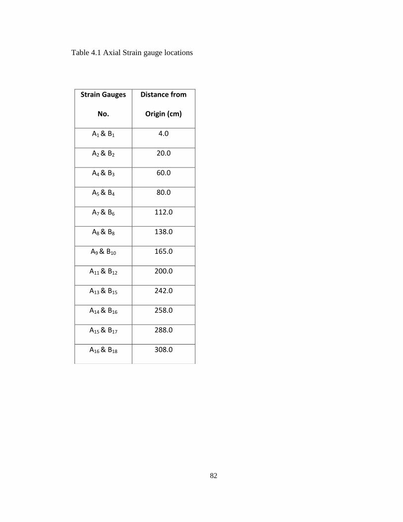
82
Table 4.1 Axial Strain gauge locations
Strain Gauges
No.
Distance from
Origin (cm)
A1 & B1 4.0
A2 & B2 20.0
A4 & B3 60.0
A5 & B4 80.0
A7 & B6 112.0
A8 & B8 138.0
A9 & B10 165.0
A11 & B12 200.0
A13 & B15 242.0
A14 & B16 258.0
A15 & B17 288.0
A16 & B18 308.0
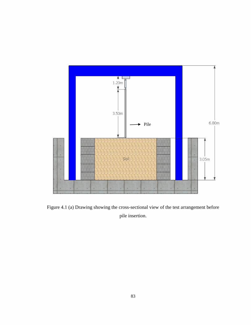
83
Figure 4.1 (a) Drawing showing the cross-sectional view of the test arrangement before
pile insertion.
Pile
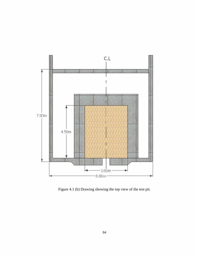
84
Figure 4.1 (b) Drawing showing the top view of the test pit.
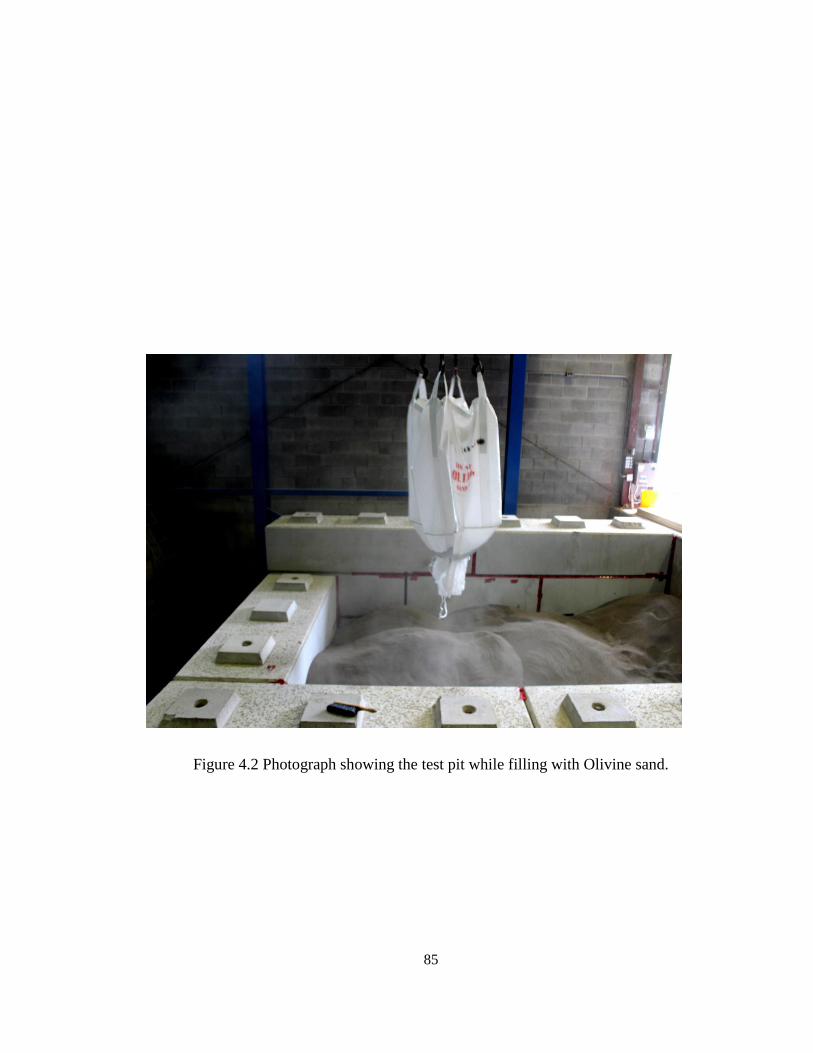
85
Figure 4.2 Photograph showing the test pit while filling with Olivine sand.
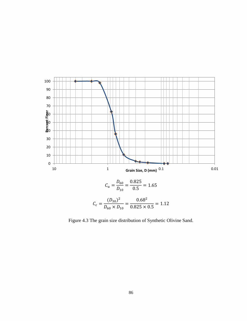
86
Figure 4.3 The grain size distribution of Synthetic Olivine Sand.
0
10
20
30
40
50
60
70
80
90
100
0.010.1110
Pe
rce
nt
Fin
er
Grain Size, D (mm)
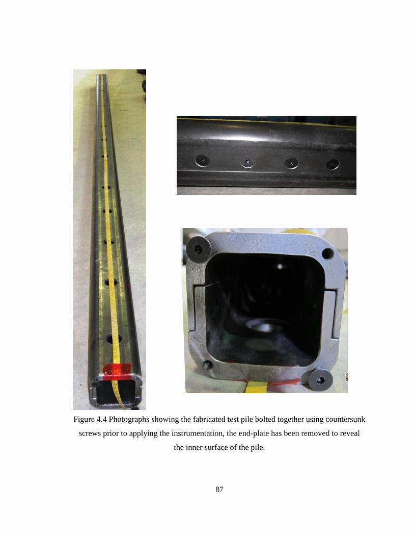
87
Figure 4.4 Photographs showing the fabricated test pile bolted together using countersunk
screws prior to applying the instrumentation, the end-plate has been removed to reveal
the inner surface of the pile.
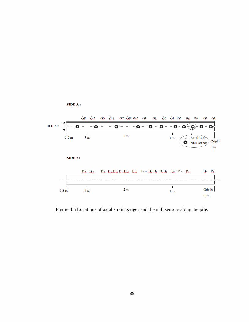
88
Figure 4.5 Locations of axial strain gauges and the null sensors along the pile.
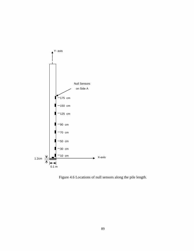
89
Y- axis
Null Sensors
on Side A
1.2cm
X-axis
0.1 m
Figure 4.6 Locations of null sensors along the pile length.
175 cm
150 cm
125 cm
90 cm
30 cm
70 cm
50 cm
10 cm
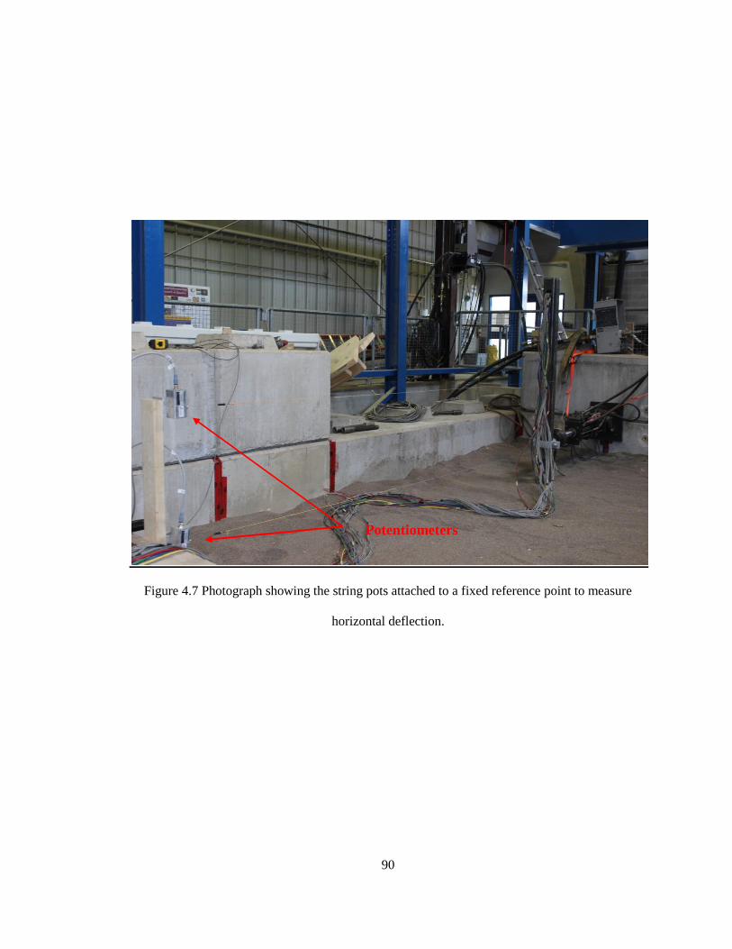
90
Figure 4.7 Photograph showing the string pots attached to a fixed reference point to measure
horizontal deflection.
Potentiometers
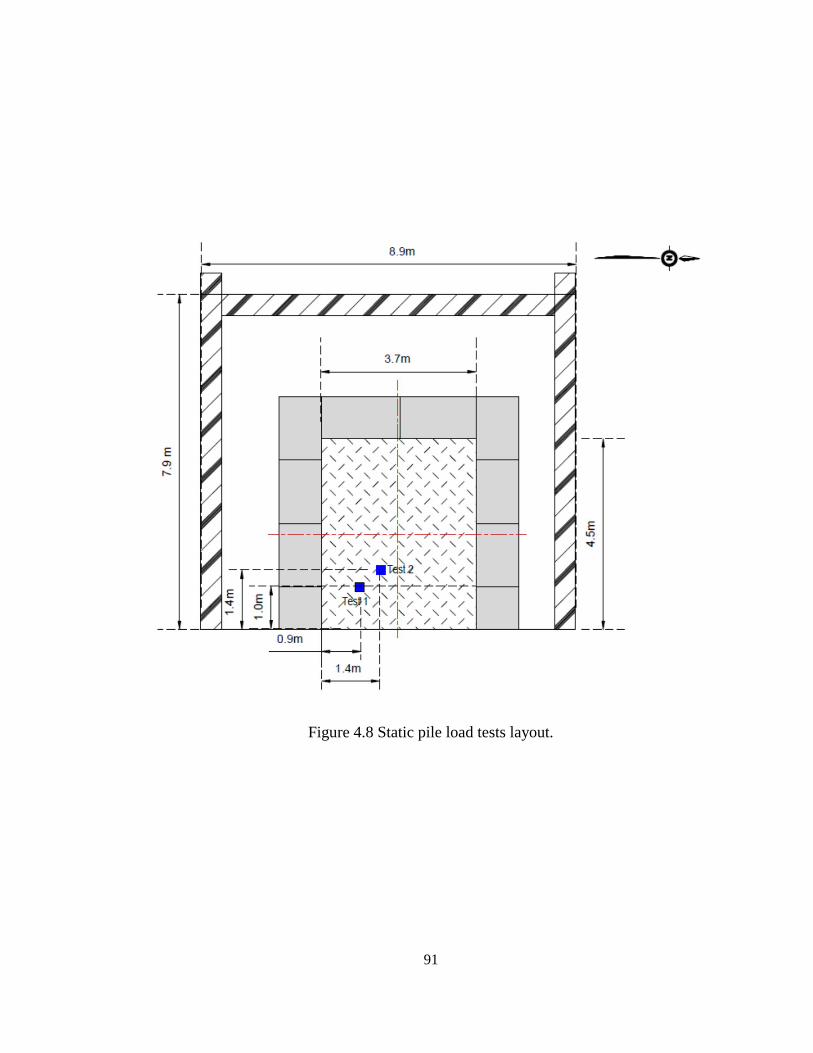
91
Figure 4.8 Static pile load tests layout.
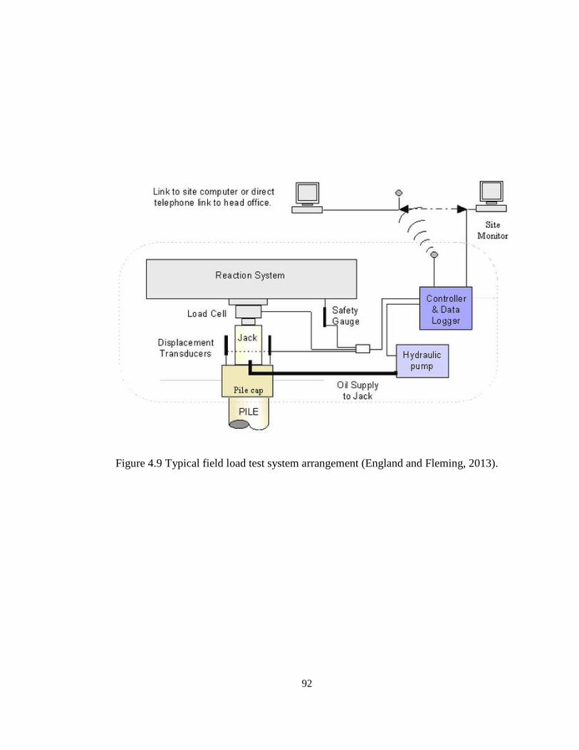
92
Figure 4.9 Typical field load test system arrangement (England and Fleming, 2013).
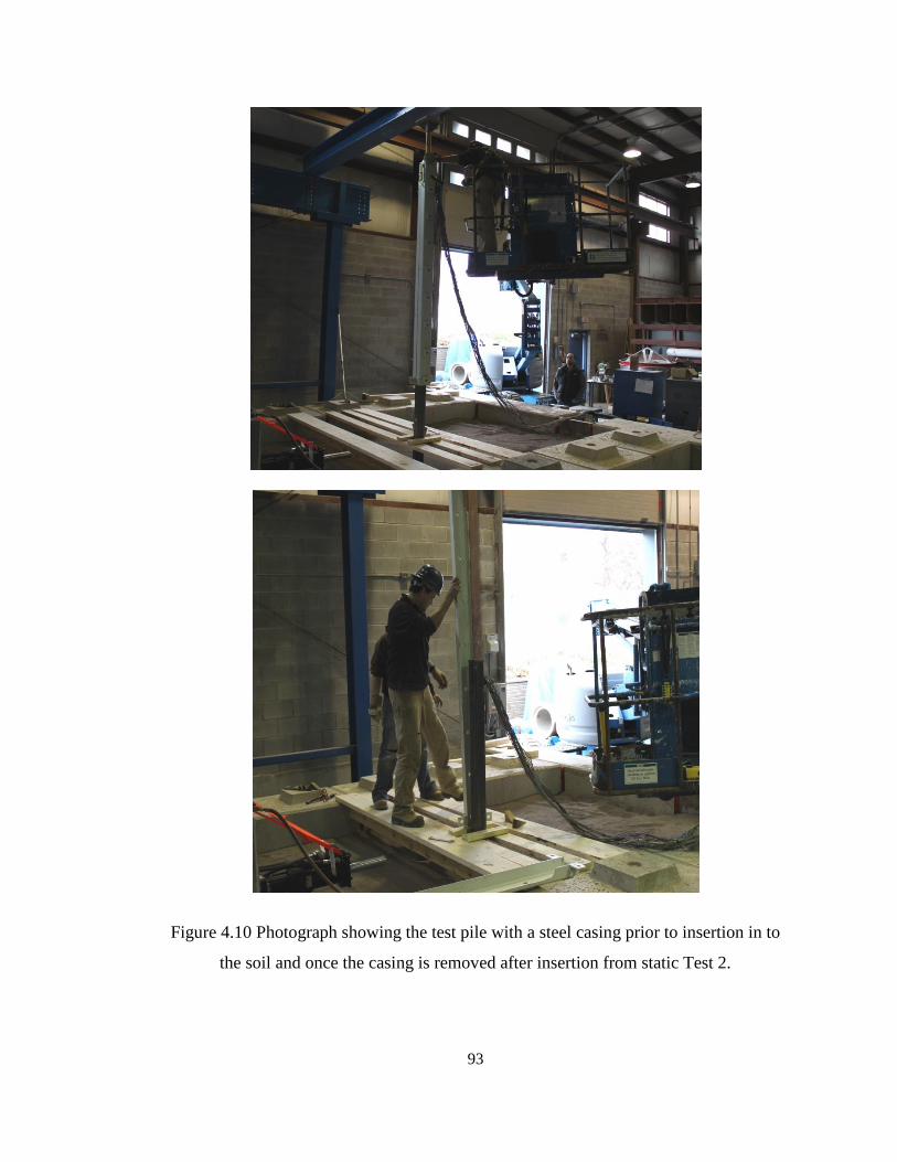
93
Figure 4.10 Photograph showing the test pile with a steel casing prior to insertion in to
the soil and once the casing is removed after insertion from static Test 2.
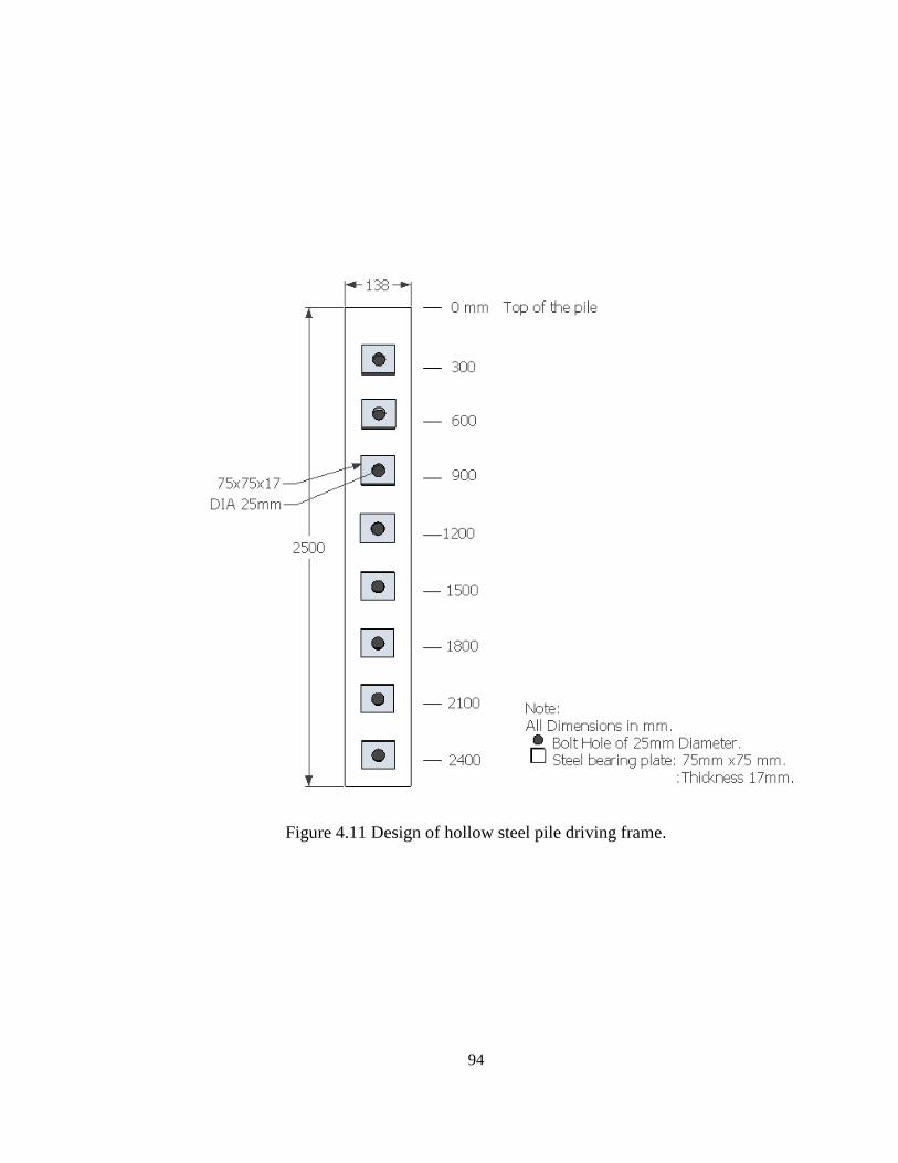
94
Figure 4.11 Design of hollow steel pile driving frame.
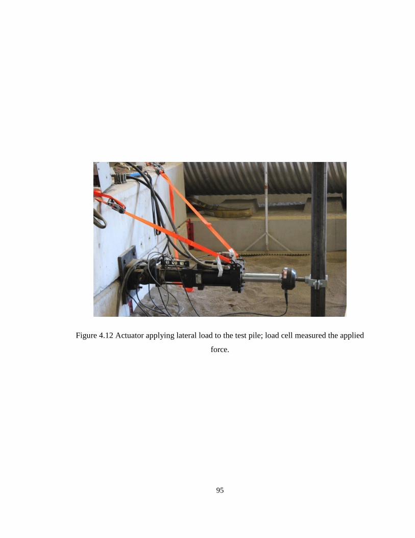
95
Figure 4.12 Actuator applying lateral load to the test pile; load cell measured the applied
force.
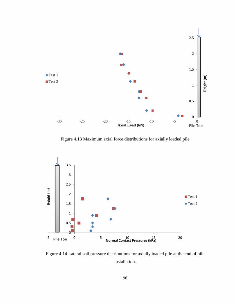
96
Figure 4.13 Maximum axial force distributions for axially loaded pile
Figure 4.14 Lateral soil pressure distributions for axially loaded pile at the end of pile
installation.
0
0.5
1
1.5
2
2.5
-30 -25 -20 -15 -10 -5 0
Hei
gh
t (m
)
Axial Load (kN)
Test 1
Test 2
Pile Toe
0
0.5
1
1.5
2
2.5
3
3.5
-5 0 5 10 15 20
He
igh
t (m
)
Normal Contact Pressures (kPa)
Test 1
Test 2
Pile Toe
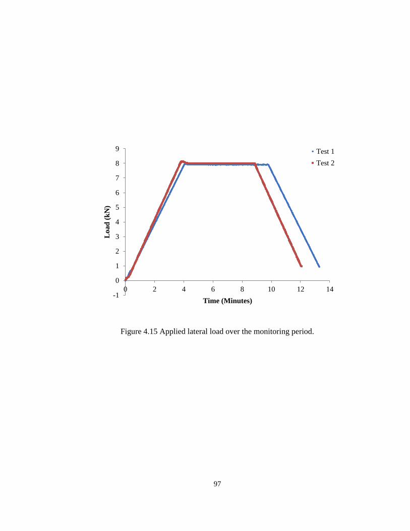
97
Figure 4.15 Applied lateral load over the monitoring period.
-1
0
1
2
3
4
5
6
7
8
9
0 2 4 6 8 10 12 14
Load
(k
N)
Time (Minutes)
Test 1
Test 2
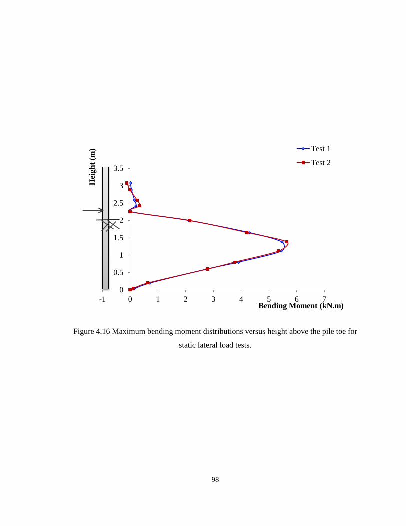
98
Figure 4.16 Maximum bending moment distributions versus height above the pile toe for
static lateral load tests.
0
0.5
1
1.5
2
2.5
3
3.5
-1 0 1 2 3 4 5 6 7
Hei
gh
t (m
)
Bending Moment (kN.m)
Test 1
Test 2
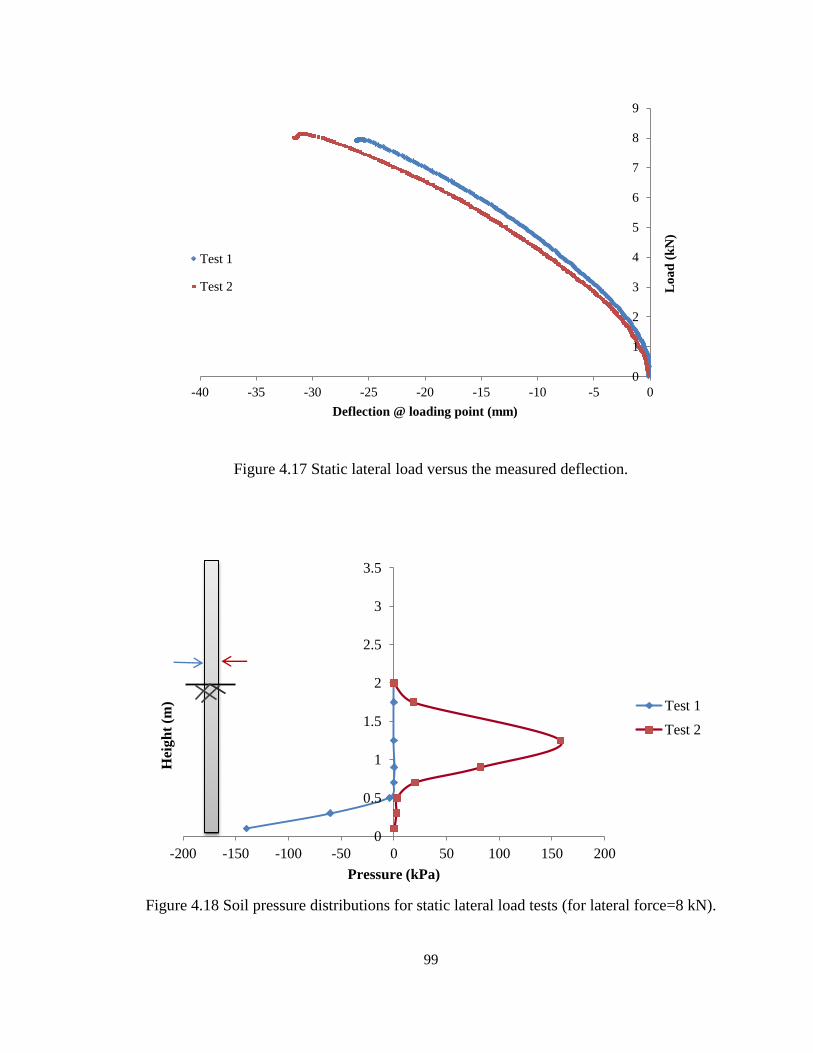
99
Figure 4.17 Static lateral load versus the measured deflection.
Figure 4.18 Soil pressure distributions for static lateral load tests (for lateral force=8 kN).
0
1
2
3
4
5
6
7
8
9
-40 -35 -30 -25 -20 -15 -10 -5 0
Lo
ad
(k
N)
Deflection @ loading point (mm)
Test 1
Test 2
0
0.5
1
1.5
2
2.5
3
3.5
-200 -150 -100 -50 0 50 100 150 200
Hei
gh
t (m
)
Pressure (kPa)
Test 1
Test 2
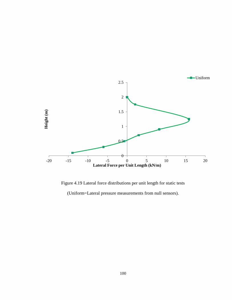
100
Figure 4.19 Lateral force distributions per unit length for static tests
(Uniform=Lateral pressure measurements from null sensors).
0
0.5
1
1.5
2
2.5
-20 -15 -10 -5 0 5 10 15 20
Hei
gh
t (m
)
Lateral Force per Unit Length (kN/m)
Uniform
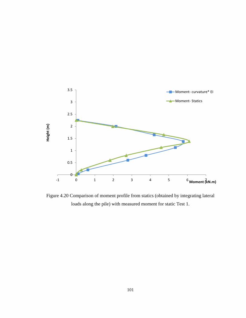
101
Figure 4.20 Comparison of moment profile from statics (obtained by integrating lateral
loads along the pile) with measured moment for static Test 1.
0
0.5
1
1.5
2
2.5
3
3.5
-1 0 1 2 3 4 5 6 7
He
igh
t (m
)
Moment (kN.m)
Moment- curvature* EI
Moment- Statics
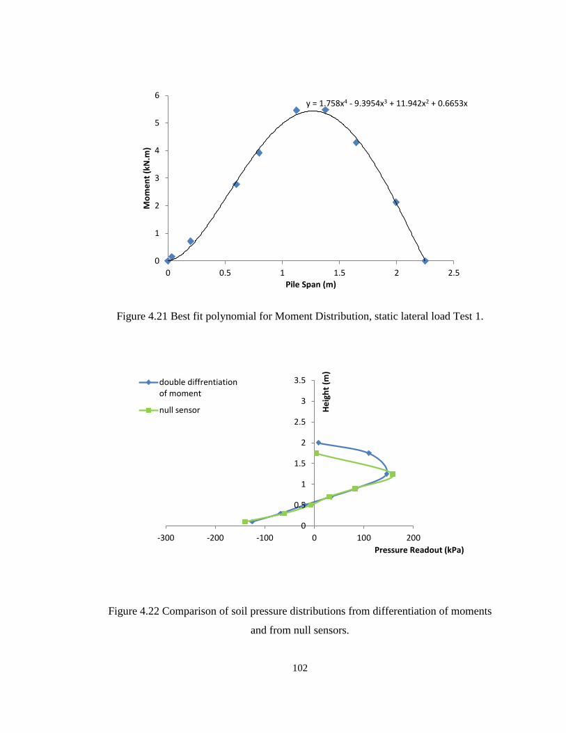
102
Figure 4.21 Best fit polynomial for Moment Distribution, static lateral load Test 1.
Figure 4.22 Comparison of soil pressure distributions from differentiation of moments
and from null sensors.
y = 1.758x4 - 9.3954x3 + 11.942x2 + 0.6653x
0
1
2
3
4
5
6
0 0.5 1 1.5 2 2.5
Mo
me
nt
(kN
.m)
Pile Span (m)
0
0.5
1
1.5
2
2.5
3
3.5
-300 -200 -100 0 100 200
He
igh
t (m
)
Pressure Readout (kPa)
double diffrentiationof moment
null sensor
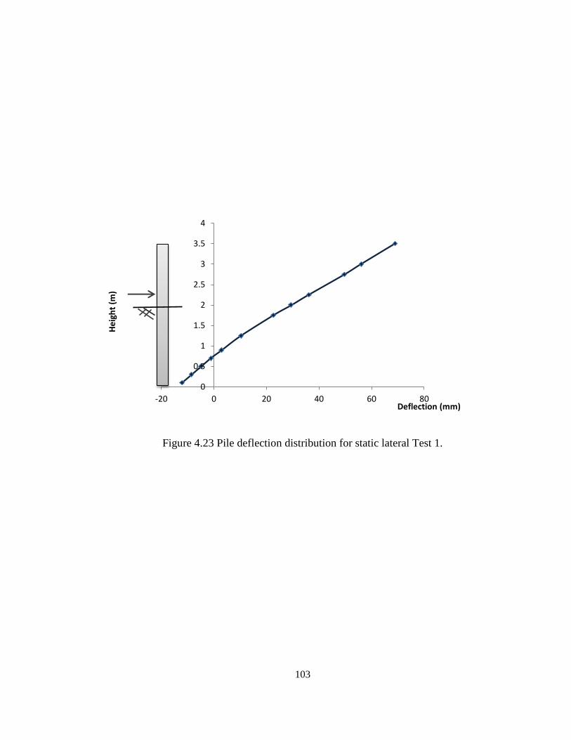
103
Figure 4.23 Pile deflection distribution for static lateral Test 1.
0
0.5
1
1.5
2
2.5
3
3.5
4
-20 0 20 40 60 80
He
igh
t (m
)
Deflection (mm)
104
Chapter 5
CYCLIC PILE LOAD TESTS
5.1 INTRODUCTION
Many piles supporting offshore structures and bridges are exposed to cyclic lateral
loading with different magnitude and period due to tide, wind, and wave actions.
Therefore, it can be important to consider pile response when subjected to cyclic lateral
loading when designing these structures (Olsen, 2011).
In general, peak moments and deflections increase with an increasing number of cycles as
well as with load magnitude (Giannakos et al., 2012). Achmus et al. (2009) noted that
during cyclic loading, the location of the plastic hinge or point of rotation moves deeper
due to soil stiffness degradation. In addition, cyclic lateral loads induce elastic and
inelastic incremental responses which depend on type of cyclic loading (one-way versus
two-way). Giannakos et al. (2012) also showed that one-way cyclic lateral loads induce
greater cumulative deformations than two-way cyclic lateral loads.
Another phenomenon that may influence pile response to cyclic lateral loading is
gapping. Gapping is the formation of an opening at the pile-soil interface near the ground
surface (Pender and Pranjoto, 1996). As the number of loading cycles and magnitude of
applied load increase, it has been reported that the failure zone enlarges and the depth of
the gap increases (Qin and Guo, 2007).
105
This chapter reports on a study of cyclic lateral loading of a test pile in sand to investigate
and interpret the physical phenomena associated with cyclic lateral loading. Although
previous studies have been conducted to examine the effects of cyclic loading on full-
scale pile tests in loose sandy soil (Reddy, 1996; Qin et al., 2007; Achmus et al., 2009;
Olsen, 2011 and Giannakos et al., 2012), a novel aspect of the present work is the
integration of high quality measurements of lateral earth pressure on one side of a test
pile using null sensors, together with more conventional measurements of moment and
deformation.
This chapter of the dissertation reports on five (5) cyclic pile load tests conducted in
loose dry sand at the Geo-Engineering Laboratory at Queen's University. The goals of the
work are to:
- examine and compare cyclic pile responses under one-way and two-way lateral
loading
- investigate the relationship between distributions of lateral pressure and bending
moment down the pile
- study the influence of embedment and load eccentricity on the pile behaviour
- investigate the effect of load level on the accumulation of permanent deformation
- examine how the kinematics (e.g. point of pile rotation) changes with load cycles,
load level, and any load reversal (two–way loading instead of one-way loading)
106
- Analyse the impact of gap formation on cyclic responses
After describing the instrumented test pile and the soil conditions, the testing program
design is discussed in relation to the project goals. The measurements and their
interpretation are then presented.
5.2 TEST SETUP
The test setup including the test pile, instrumentation and material description are the
same as those used for the monotonic load tests presented in Chapter 4. However, a
summary of the test set up for the cyclic loading experiments is provided in the following
subsections.
5.2.1 Soil Material
All of the cyclic lateral loading tests were performed on the test pile installed within dry
Olivine Sand. The material is poorly graded sand with grain size distribution presented in
Figure 4.3. The unit weight of the loose Olivine Sand is 13 kN/m3 and the angle of
friction is 40 degrees (Lapos and Moore, 2002). This soil was loosely placed in a test pit
4.5 m wide, 3.6 m long and 3.0 m deep.
5.2.2 Test Pile and Instrumentation
The pile is a close-ended hollow square steel tube with a nominal size of HSS
102x102x13 mm and length of 3.5 m (Canadian Institute of Steel Construction, 2007).
The pile was fabricated from a hollow steel section of rectangular cross section which
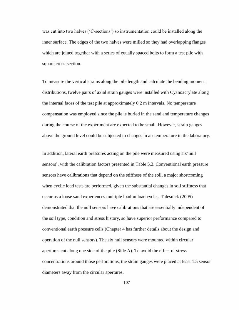
107
was cut into two halves (‘C-sections’) so instrumentation could be installed along the
inner surface. The edges of the two halves were milled so they had overlapping flanges
which are joined together with a series of equally spaced bolts to form a test pile with
square cross-section.
To measure the vertical strains along the pile length and calculate the bending moment
distributions, twelve pairs of axial strain gauges were installed with Cyanoacrylate along
the internal faces of the test pile at approximately 0.2 m intervals. No temperature
compensation was employed since the pile is buried in the sand and temperature changes
during the course of the experiment are expected to be small. However, strain gauges
above the ground level could be subjected to changes in air temperature in the laboratory.
In addition, lateral earth pressures acting on the pile were measured using six‘null
sensors’, with the calibration factors presented in Table 5.2. Conventional earth pressure
sensors have calibrations that depend on the stiffness of the soil, a major shortcoming
when cyclic load tests are performed, given the substantial changes in soil stiffness that
occur as a loose sand experiences multiple load-unload cycles. Talesnick (2005)
demonstrated that the null sensors have calibrations that are essentially independent of
the soil type, condition and stress history, so have superior performance compared to
conventional earth pressure cells (Chapter 4 has further details about the design and
operation of the null sensors). The six null sensors were mounted within circular
apertures cut along one side of the pile (Side A). To avoid the effect of stress
concentrations around those perforations, the strain gauges were placed at least 1.5 sensor
diameters away from the circular apertures.
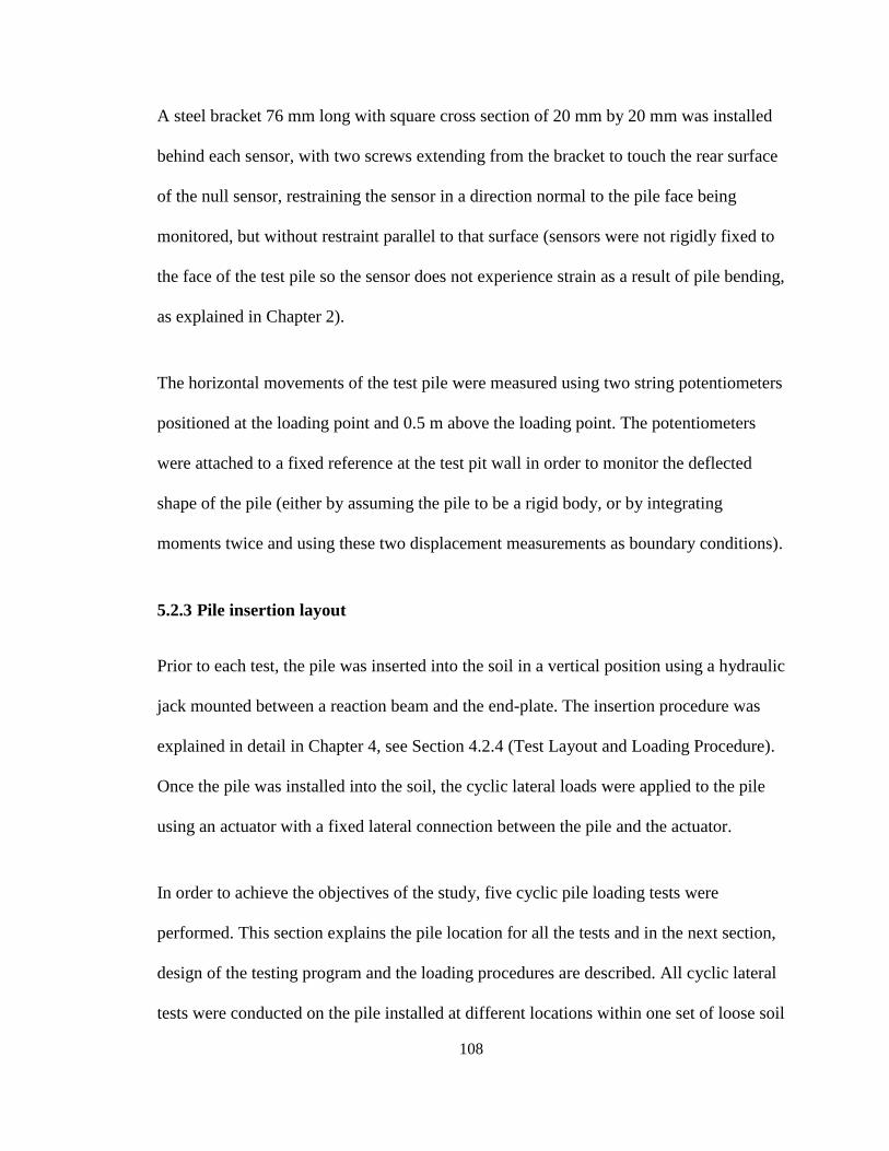
108
A steel bracket 76 mm long with square cross section of 20 mm by 20 mm was installed
behind each sensor, with two screws extending from the bracket to touch the rear surface
of the null sensor, restraining the sensor in a direction normal to the pile face being
monitored, but without restraint parallel to that surface (sensors were not rigidly fixed to
the face of the test pile so the sensor does not experience strain as a result of pile bending,
as explained in Chapter 2).
The horizontal movements of the test pile were measured using two string potentiometers
positioned at the loading point and 0.5 m above the loading point. The potentiometers
were attached to a fixed reference at the test pit wall in order to monitor the deflected
shape of the pile (either by assuming the pile to be a rigid body, or by integrating
moments twice and using these two displacement measurements as boundary conditions).
5.2.3 Pile insertion layout
Prior to each test, the pile was inserted into the soil in a vertical position using a hydraulic
jack mounted between a reaction beam and the end-plate. The insertion procedure was
explained in detail in Chapter 4, see Section 4.2.4 (Test Layout and Loading Procedure).
Once the pile was installed into the soil, the cyclic lateral loads were applied to the pile
using an actuator with a fixed lateral connection between the pile and the actuator.
In order to achieve the objectives of the study, five cyclic pile loading tests were
performed. This section explains the pile location for all the tests and in the next section,
design of the testing program and the loading procedures are described. All cyclic lateral
tests were conducted on the pile installed at different locations within one set of loose soil
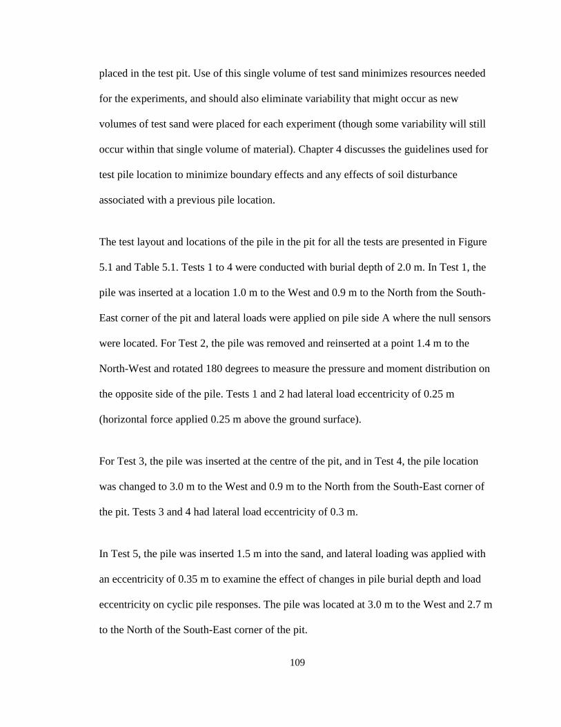
109
placed in the test pit. Use of this single volume of test sand minimizes resources needed
for the experiments, and should also eliminate variability that might occur as new
volumes of test sand were placed for each experiment (though some variability will still
occur within that single volume of material). Chapter 4 discusses the guidelines used for
test pile location to minimize boundary effects and any effects of soil disturbance
associated with a previous pile location.
The test layout and locations of the pile in the pit for all the tests are presented in Figure
5.1 and Table 5.1. Tests 1 to 4 were conducted with burial depth of 2.0 m. In Test 1, the
pile was inserted at a location 1.0 m to the West and 0.9 m to the North from the South-
East corner of the pit and lateral loads were applied on pile side A where the null sensors
were located. For Test 2, the pile was removed and reinserted at a point 1.4 m to the
North-West and rotated 180 degrees to measure the pressure and moment distribution on
the opposite side of the pile. Tests 1 and 2 had lateral load eccentricity of 0.25 m
(horizontal force applied 0.25 m above the ground surface).
For Test 3, the pile was inserted at the centre of the pit, and in Test 4, the pile location
was changed to 3.0 m to the West and 0.9 m to the North from the South-East corner of
the pit. Tests 3 and 4 had lateral load eccentricity of 0.3 m.
In Test 5, the pile was inserted 1.5 m into the sand, and lateral loading was applied with
an eccentricity of 0.35 m to examine the effect of changes in pile burial depth and load
eccentricity on cyclic pile responses. The pile was located at 3.0 m to the West and 2.7 m
to the North of the South-East corner of the pit.
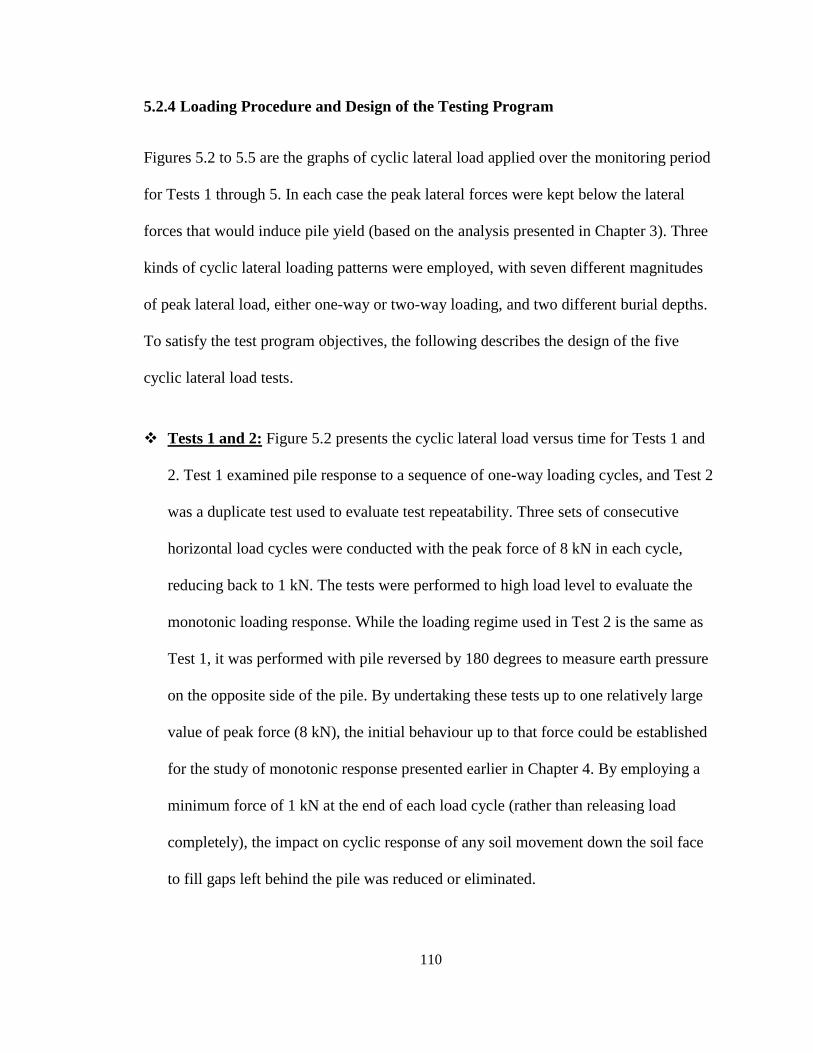
110
5.2.4 Loading Procedure and Design of the Testing Program
Figures 5.2 to 5.5 are the graphs of cyclic lateral load applied over the monitoring period
for Tests 1 through 5. In each case the peak lateral forces were kept below the lateral
forces that would induce pile yield (based on the analysis presented in Chapter 3). Three
kinds of cyclic lateral loading patterns were employed, with seven different magnitudes
of peak lateral load, either one-way or two-way loading, and two different burial depths.
To satisfy the test program objectives, the following describes the design of the five
cyclic lateral load tests.
Tests 1 and 2: Figure 5.2 presents the cyclic lateral load versus time for Tests 1 and
2. Test 1 examined pile response to a sequence of one-way loading cycles, and Test 2
was a duplicate test used to evaluate test repeatability. Three sets of consecutive
horizontal load cycles were conducted with the peak force of 8 kN in each cycle,
reducing back to 1 kN. The tests were performed to high load level to evaluate the
monotonic loading response. While the loading regime used in Test 2 is the same as
Test 1, it was performed with pile reversed by 180 degrees to measure earth pressure
on the opposite side of the pile. By undertaking these tests up to one relatively large
value of peak force (8 kN), the initial behaviour up to that force could be established
for the study of monotonic response presented earlier in Chapter 4. By employing a
minimum force of 1 kN at the end of each load cycle (rather than releasing load
completely), the impact on cyclic response of any soil movement down the soil face
to fill gaps left behind the pile was reduced or eliminated.
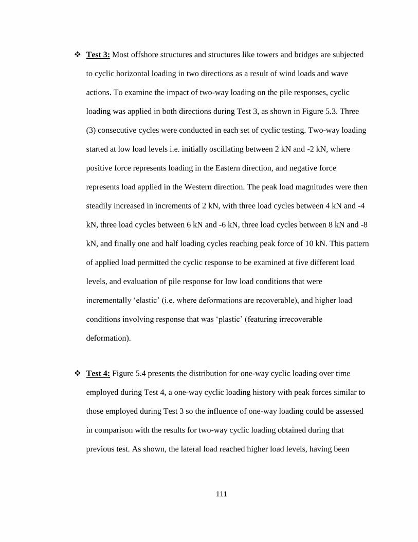
111
Test 3: Most offshore structures and structures like towers and bridges are subjected
to cyclic horizontal loading in two directions as a result of wind loads and wave
actions. To examine the impact of two-way loading on the pile responses, cyclic
loading was applied in both directions during Test 3, as shown in Figure 5.3. Three
(3) consecutive cycles were conducted in each set of cyclic testing. Two-way loading
started at low load levels i.e. initially oscillating between 2 kN and -2 kN, where
positive force represents loading in the Eastern direction, and negative force
represents load applied in the Western direction. The peak load magnitudes were then
steadily increased in increments of 2 kN, with three load cycles between 4 kN and -4
kN, three load cycles between 6 kN and -6 kN, three load cycles between 8 kN and -8
kN, and finally one and half loading cycles reaching peak force of 10 kN. This pattern
of applied load permitted the cyclic response to be examined at five different load
levels, and evaluation of pile response for low load conditions that were
incrementally ‘elastic’ (i.e. where deformations are recoverable), and higher load
conditions involving response that was ‘plastic’ (featuring irrecoverable
deformation).
Test 4: Figure 5.4 presents the distribution for one-way cyclic loading over time
employed during Test 4, a one-way cyclic loading history with peak forces similar to
those employed during Test 3 so the influence of one-way loading could be assessed
in comparison with the results for two-way cyclic loading obtained during that
previous test. As shown, the lateral load reached higher load levels, having been
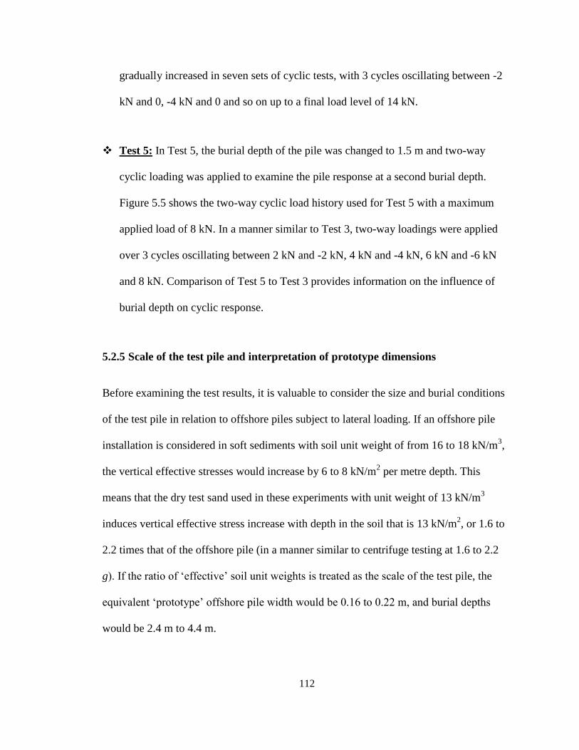
112
gradually increased in seven sets of cyclic tests, with 3 cycles oscillating between -2
kN and 0, -4 kN and 0 and so on up to a final load level of 14 kN.
Test 5: In Test 5, the burial depth of the pile was changed to 1.5 m and two-way
cyclic loading was applied to examine the pile response at a second burial depth.
Figure 5.5 shows the two-way cyclic load history used for Test 5 with a maximum
applied load of 8 kN. In a manner similar to Test 3, two-way loadings were applied
over 3 cycles oscillating between 2 kN and -2 kN, 4 kN and -4 kN, 6 kN and -6 kN
and 8 kN. Comparison of Test 5 to Test 3 provides information on the influence of
burial depth on cyclic response.
5.2.5 Scale of the test pile and interpretation of prototype dimensions
Before examining the test results, it is valuable to consider the size and burial conditions
of the test pile in relation to offshore piles subject to lateral loading. If an offshore pile
installation is considered in soft sediments with soil unit weight of from 16 to 18 kN/m3,
the vertical effective stresses would increase by 6 to 8 kN/m2 per metre depth. This
means that the dry test sand used in these experiments with unit weight of 13 kN/m3
induces vertical effective stress increase with depth in the soil that is 13 kN/m2, or 1.6 to
2.2 times that of the offshore pile (in a manner similar to centrifuge testing at 1.6 to 2.2
g). If the ratio of ‘effective’ soil unit weights is treated as the scale of the test pile, the
equivalent ‘prototype’ offshore pile width would be 0.16 to 0.22 m, and burial depths
would be 2.4 m to 4.4 m.
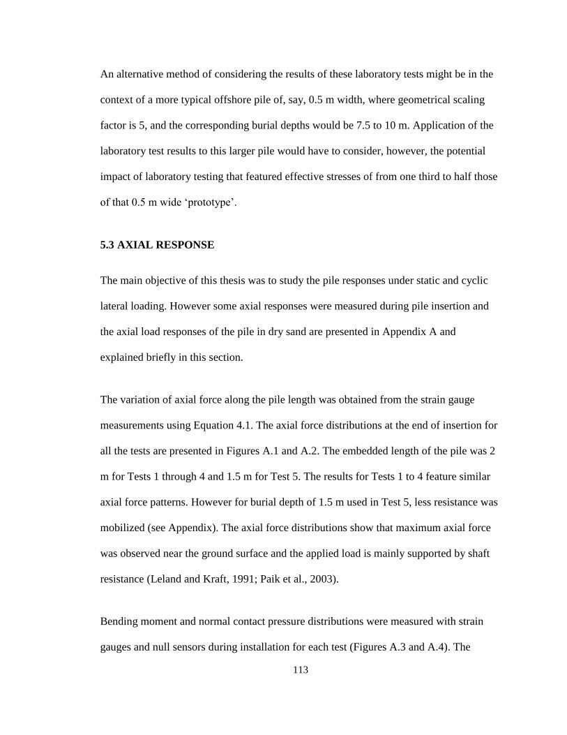
113
An alternative method of considering the results of these laboratory tests might be in the
context of a more typical offshore pile of, say, 0.5 m width, where geometrical scaling
factor is 5, and the corresponding burial depths would be 7.5 to 10 m. Application of the
laboratory test results to this larger pile would have to consider, however, the potential
impact of laboratory testing that featured effective stresses of from one third to half those
of that 0.5 m wide ‘prototype’.
5.3 AXIAL RESPONSE
The main objective of this thesis was to study the pile responses under static and cyclic
lateral loading. However some axial responses were measured during pile insertion and
the axial load responses of the pile in dry sand are presented in Appendix A and
explained briefly in this section.
The variation of axial force along the pile length was obtained from the strain gauge
measurements using Equation 4.1. The axial force distributions at the end of insertion for
all the tests are presented in Figures A.1 and A.2. The embedded length of the pile was 2
m for Tests 1 through 4 and 1.5 m for Test 5. The results for Tests 1 to 4 feature similar
axial force patterns. However for burial depth of 1.5 m used in Test 5, less resistance was
mobilized (see Appendix). The axial force distributions show that maximum axial force
was observed near the ground surface and the applied load is mainly supported by shaft
resistance (Leland and Kraft, 1991; Paik et al., 2003).
Bending moment and normal contact pressure distributions were measured with strain
gauges and null sensors during installation for each test (Figures A.3 and A.4). The
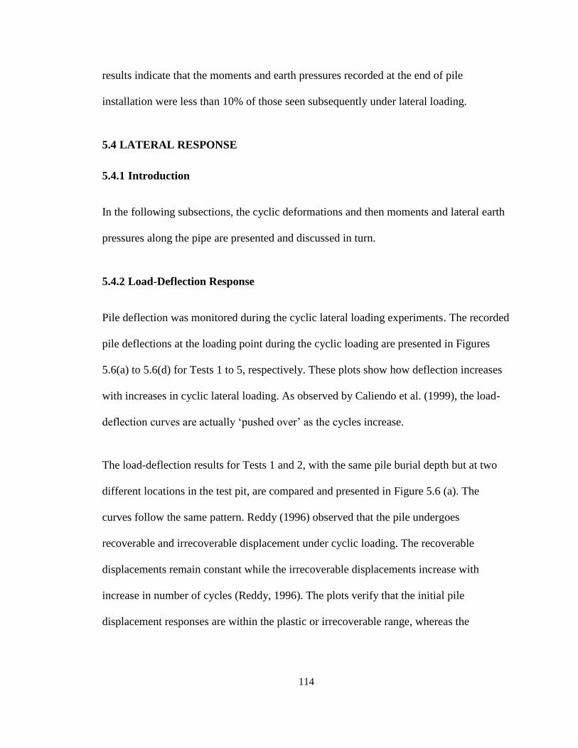
114
results indicate that the moments and earth pressures recorded at the end of pile
installation were less than 10% of those seen subsequently under lateral loading.
5.4 LATERAL RESPONSE
5.4.1 Introduction
In the following subsections, the cyclic deformations and then moments and lateral earth
pressures along the pipe are presented and discussed in turn.
5.4.2 Load-Deflection Response
Pile deflection was monitored during the cyclic lateral loading experiments. The recorded
pile deflections at the loading point during the cyclic loading are presented in Figures
5.6(a) to 5.6(d) for Tests 1 to 5, respectively. These plots show how deflection increases
with increases in cyclic lateral loading. As observed by Caliendo et al. (1999), the load-
deflection curves are actually ‘pushed over’ as the cycles increase.
The load-deflection results for Tests 1 and 2, with the same pile burial depth but at two
different locations in the test pit, are compared and presented in Figure 5.6 (a). The
curves follow the same pattern. Reddy (1996) observed that the pile undergoes
recoverable and irrecoverable displacement under cyclic loading. The recoverable
displacements remain constant while the irrecoverable displacements increase with
increase in number of cycles (Reddy, 1996). The plots verify that the initial pile
displacement responses are within the plastic or irrecoverable range, whereas the
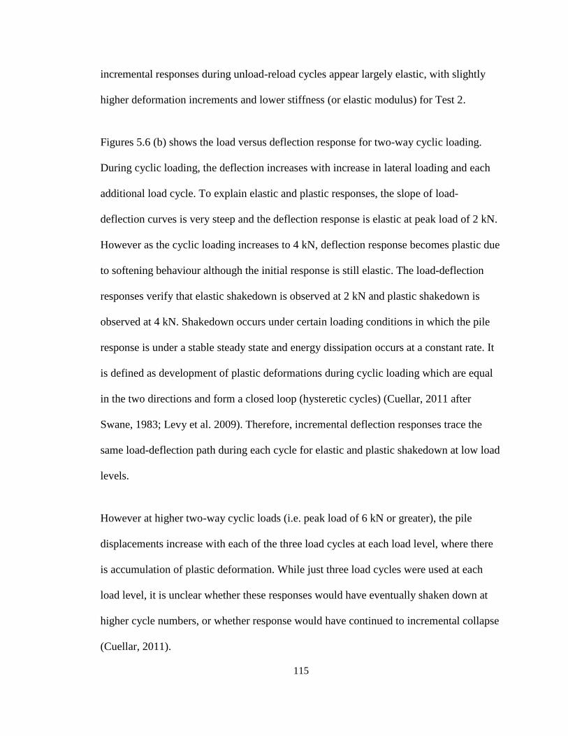
115
incremental responses during unload-reload cycles appear largely elastic, with slightly
higher deformation increments and lower stiffness (or elastic modulus) for Test 2.
Figures 5.6 (b) shows the load versus deflection response for two-way cyclic loading.
During cyclic loading, the deflection increases with increase in lateral loading and each
additional load cycle. To explain elastic and plastic responses, the slope of load-
deflection curves is very steep and the deflection response is elastic at peak load of 2 kN.
However as the cyclic loading increases to 4 kN, deflection response becomes plastic due
to softening behaviour although the initial response is still elastic. The load-deflection
responses verify that elastic shakedown is observed at 2 kN and plastic shakedown is
observed at 4 kN. Shakedown occurs under certain loading conditions in which the pile
response is under a stable steady state and energy dissipation occurs at a constant rate. It
is defined as development of plastic deformations during cyclic loading which are equal
in the two directions and form a closed loop (hysteretic cycles) (Cuellar, 2011 after
Swane, 1983; Levy et al. 2009). Therefore, incremental deflection responses trace the
same load-deflection path during each cycle for elastic and plastic shakedown at low load
levels.
However at higher two-way cyclic loads (i.e. peak load of 6 kN or greater), the pile
displacements increase with each of the three load cycles at each load level, where there
is accumulation of plastic deformation. While just three load cycles were used at each
load level, it is unclear whether these responses would have eventually shaken down at
higher cycle numbers, or whether response would have continued to incremental collapse
(Cuellar, 2011).
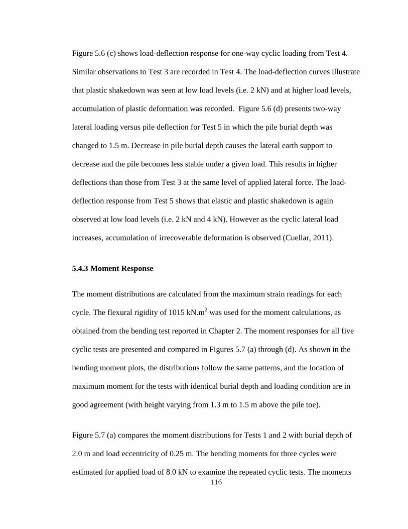
116
Figure 5.6 (c) shows load-deflection response for one-way cyclic loading from Test 4.
Similar observations to Test 3 are recorded in Test 4. The load-deflection curves illustrate
that plastic shakedown was seen at low load levels (i.e. 2 kN) and at higher load levels,
accumulation of plastic deformation was recorded. Figure 5.6 (d) presents two-way
lateral loading versus pile deflection for Test 5 in which the pile burial depth was
changed to 1.5 m. Decrease in pile burial depth causes the lateral earth support to
decrease and the pile becomes less stable under a given load. This results in higher
deflections than those from Test 3 at the same level of applied lateral force. The load-
deflection response from Test 5 shows that elastic and plastic shakedown is again
observed at low load levels (i.e. 2 kN and 4 kN). However as the cyclic lateral load
increases, accumulation of irrecoverable deformation is observed (Cuellar, 2011).
5.4.3 Moment Response
The moment distributions are calculated from the maximum strain readings for each
cycle. The flexural rigidity of 1015 kN.m2 was used for the moment calculations, as
obtained from the bending test reported in Chapter 2. The moment responses for all five
cyclic tests are presented and compared in Figures 5.7 (a) through (d). As shown in the
bending moment plots, the distributions follow the same patterns, and the location of
maximum moment for the tests with identical burial depth and loading condition are in
good agreement (with height varying from 1.3 m to 1.5 m above the pile toe).
Figure 5.7 (a) compares the moment distributions for Tests 1 and 2 with burial depth of
2.0 m and load eccentricity of 0.25 m. The bending moments for three cycles were
estimated for applied load of 8.0 kN to examine the repeated cyclic tests. The moments
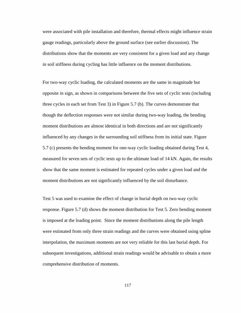
117
were associated with pile installation and therefore, thermal effects might influence strain
gauge readings, particularly above the ground surface (see earlier discussion). The
distributions show that the moments are very consistent for a given load and any change
in soil stiffness during cycling has little influence on the moment distributions.
For two-way cyclic loading, the calculated moments are the same in magnitude but
opposite in sign, as shown in comparisons between the five sets of cyclic tests (including
three cycles in each set from Test 3) in Figure 5.7 (b). The curves demonstrate that
though the deflection responses were not similar during two-way loading, the bending
moment distributions are almost identical in both directions and are not significantly
influenced by any changes in the surrounding soil stiffness from its initial state. Figure
5.7 (c) presents the bending moment for one-way cyclic loading obtained during Test 4,
measured for seven sets of cyclic tests up to the ultimate load of 14 kN. Again, the results
show that the same moment is estimated for repeated cycles under a given load and the
moment distributions are not significantly influenced by the soil disturbance.
Test 5 was used to examine the effect of change in burial depth on two-way cyclic
response. Figure 5.7 (d) shows the moment distribution for Test 5. Zero bending moment
is imposed at the loading point. Since the moment distributions along the pile length
were estimated from only three strain readings and the curves were obtained using spline
interpolation, the maximum moments are not very reliable for this last burial depth. For
subsequent investigations, additional strain readings would be advisable to obtain a more
comprehensive distribution of moments.
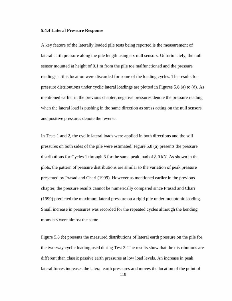
118
5.4.4 Lateral Pressure Response
A key feature of the laterally loaded pile tests being reported is the measurement of
lateral earth pressure along the pile length using six null sensors. Unfortunately, the null
sensor mounted at height of 0.1 m from the pile toe malfunctioned and the pressure
readings at this location were discarded for some of the loading cycles. The results for
pressure distributions under cyclic lateral loadings are plotted in Figures 5.8 (a) to (d). As
mentioned earlier in the previous chapter, negative pressures denote the pressure reading
when the lateral load is pushing in the same direction as stress acting on the null sensors
and positive pressures denote the reverse.
In Tests 1 and 2, the cyclic lateral loads were applied in both directions and the soil
pressures on both sides of the pile were estimated. Figure 5.8 (a) presents the pressure
distributions for Cycles 1 through 3 for the same peak load of 8.0 kN. As shown in the
plots, the pattern of pressure distributions are similar to the variation of peak pressure
presented by Prasad and Chari (1999). However as mentioned earlier in the previous
chapter, the pressure results cannot be numerically compared since Prasad and Chari
(1999) predicted the maximum lateral pressure on a rigid pile under monotonic loading.
Small increase in pressures was recorded for the repeated cycles although the bending
moments were almost the same.
Figure 5.8 (b) presents the measured distributions of lateral earth pressure on the pile for
the two-way cyclic loading used during Test 3. The results show that the distributions are
different than classic passive earth pressures at low load levels. An increase in peak
lateral forces increases the lateral earth pressures and moves the location of the point of
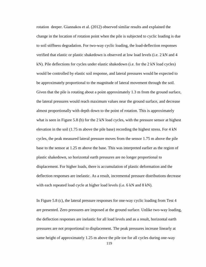
119
rotation deeper. Giannakos et al. (2012) observed similar results and explained the
change in the location of rotation point when the pile is subjected to cyclic loading is due
to soil stiffness degradation. For two-way cyclic loading, the load-deflection responses
verified that elastic or plastic shakedown is observed at low load levels (i.e. 2 kN and 4
kN). Pile deflections for cycles under elastic shakedown (i.e. for the 2 kN load cycles)
would be controlled by elastic soil response, and lateral pressures would be expected to
be approximately proportional to the magnitude of lateral movement through the soil.
Given that the pile is rotating about a point approximately 1.3 m from the ground surface,
the lateral pressures would reach maximum values near the ground surface, and decrease
almost proportionally with depth down to the point of rotation. This is approximately
what is seen in Figure 5.8 (b) for the 2 kN load cycles, with the pressure sensor at highest
elevation in the soil (1.75 m above the pile base) recording the highest stress. For 4 kN
cycles, the peak measured lateral pressure moves from the sensor 1.75 m above the pile
base to the sensor at 1.25 m above the base. This was interpreted earlier as the region of
plastic shakedown, so horizontal earth pressures are no longer proportional to
displacement. For higher loads, there is accumulation of plastic deformation and the
deflection responses are inelastic. As a result, incremental pressure distributions decrease
with each repeated load cycle at higher load levels (i.e. 6 kN and 8 kN).
In Figure 5.8 (c), the lateral pressure responses for one-way cyclic loading from Test 4
are presented. Zero pressures are imposed at the ground surface. Unlike two-way loading,
the deflection responses are inelastic for all load levels and as a result, horizontal earth
pressures are not proportional to displacement. The peak pressures increase linearly at
same height of approximately 1.25 m above the pile toe for all cycles during one-way
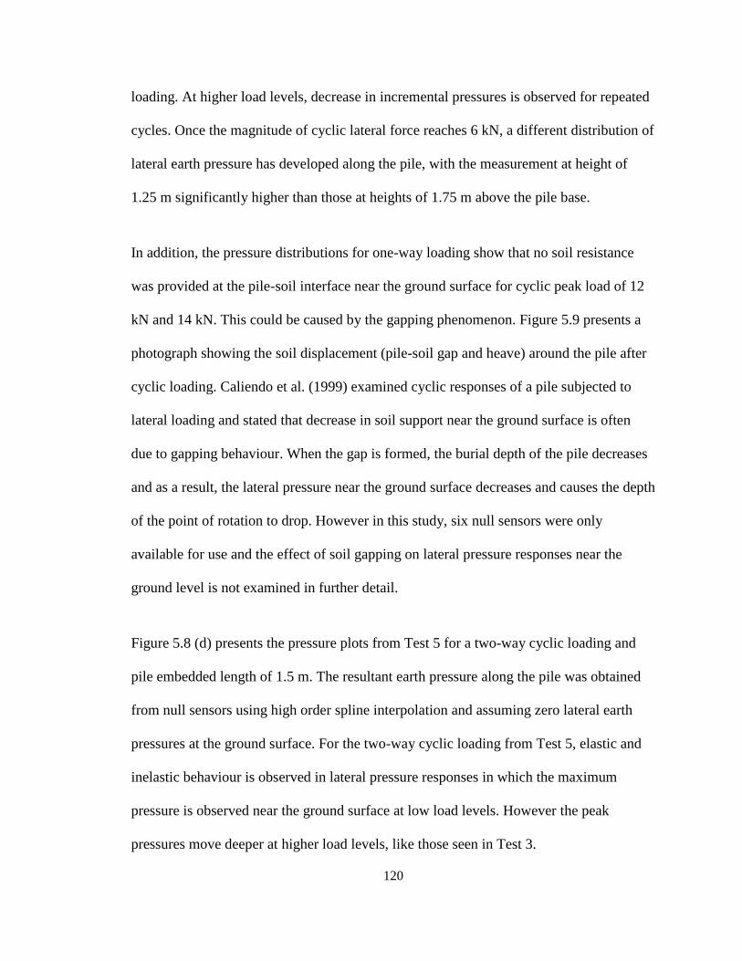
120
loading. At higher load levels, decrease in incremental pressures is observed for repeated
cycles. Once the magnitude of cyclic lateral force reaches 6 kN, a different distribution of
lateral earth pressure has developed along the pile, with the measurement at height of
1.25 m significantly higher than those at heights of 1.75 m above the pile base.
In addition, the pressure distributions for one-way loading show that no soil resistance
was provided at the pile-soil interface near the ground surface for cyclic peak load of 12
kN and 14 kN. This could be caused by the gapping phenomenon. Figure 5.9 presents a
photograph showing the soil displacement (pile-soil gap and heave) around the pile after
cyclic loading. Caliendo et al. (1999) examined cyclic responses of a pile subjected to
lateral loading and stated that decrease in soil support near the ground surface is often
due to gapping behaviour. When the gap is formed, the burial depth of the pile decreases
and as a result, the lateral pressure near the ground surface decreases and causes the depth
of the point of rotation to drop. However in this study, six null sensors were only
available for use and the effect of soil gapping on lateral pressure responses near the
ground level is not examined in further detail.
Figure 5.8 (d) presents the pressure plots from Test 5 for a two-way cyclic loading and
pile embedded length of 1.5 m. The resultant earth pressure along the pile was obtained
from null sensors using high order spline interpolation and assuming zero lateral earth
pressures at the ground surface. For the two-way cyclic loading from Test 5, elastic and
inelastic behaviour is observed in lateral pressure responses in which the maximum
pressure is observed near the ground surface at low load levels. However the peak
pressures move deeper at higher load levels, like those seen in Test 3.
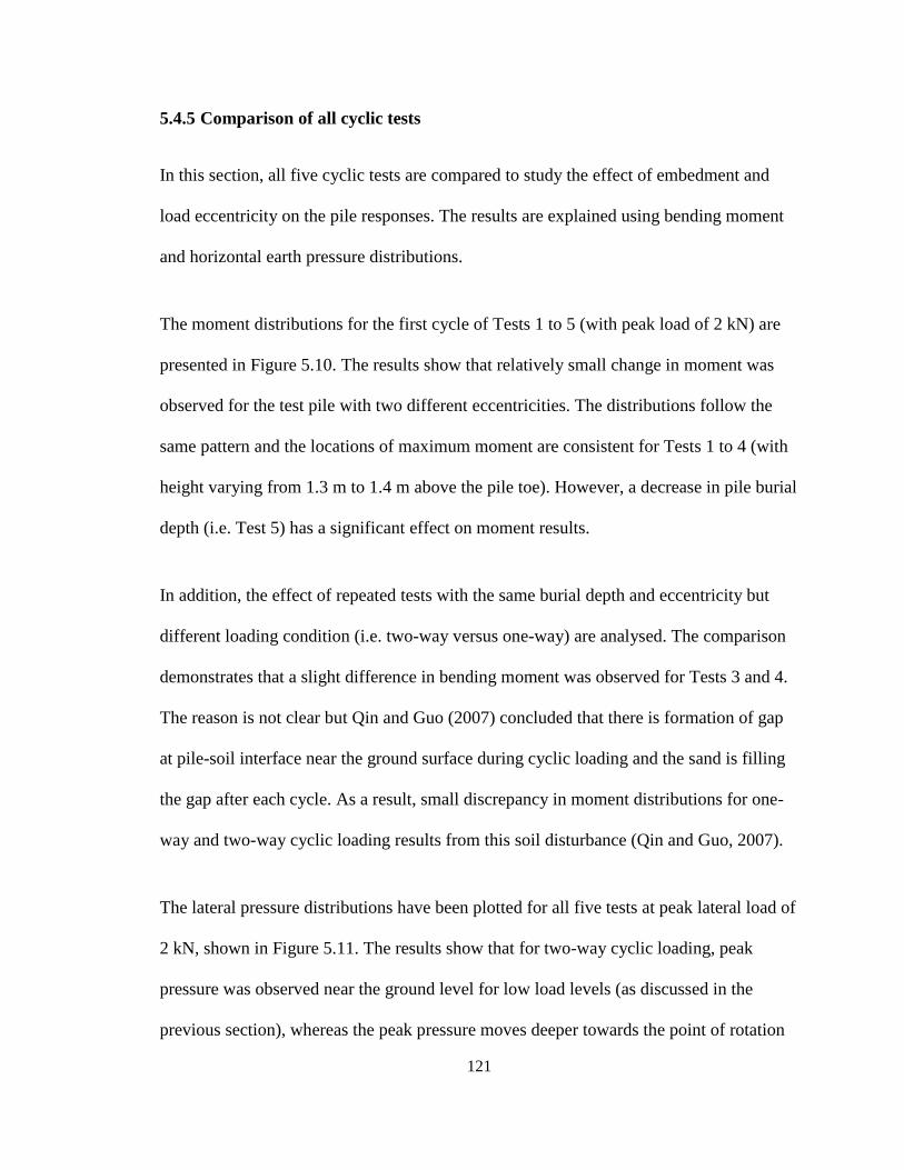
121
5.4.5 Comparison of all cyclic tests
In this section, all five cyclic tests are compared to study the effect of embedment and
load eccentricity on the pile responses. The results are explained using bending moment
and horizontal earth pressure distributions.
The moment distributions for the first cycle of Tests 1 to 5 (with peak load of 2 kN) are
presented in Figure 5.10. The results show that relatively small change in moment was
observed for the test pile with two different eccentricities. The distributions follow the
same pattern and the locations of maximum moment are consistent for Tests 1 to 4 (with
height varying from 1.3 m to 1.4 m above the pile toe). However, a decrease in pile burial
depth (i.e. Test 5) has a significant effect on moment results.
In addition, the effect of repeated tests with the same burial depth and eccentricity but
different loading condition (i.e. two-way versus one-way) are analysed. The comparison
demonstrates that a slight difference in bending moment was observed for Tests 3 and 4.
The reason is not clear but Qin and Guo (2007) concluded that there is formation of gap
at pile-soil interface near the ground surface during cyclic loading and the sand is filling
the gap after each cycle. As a result, small discrepancy in moment distributions for one-
way and two-way cyclic loading results from this soil disturbance (Qin and Guo, 2007).
The lateral pressure distributions have been plotted for all five tests at peak lateral load of
2 kN, shown in Figure 5.11. The results show that for two-way cyclic loading, peak
pressure was observed near the ground level for low load levels (as discussed in the
previous section), whereas the peak pressure moves deeper towards the point of rotation
122
for one-way loading. Similar to moment responses, the lateral pressure responses are
sensitive to change in embedment and loading condition. However, the effect of changes
in load eccentricity on pressure responses is insignificant.
5.5 SUMMARY
Five experiments have been conducted to investigate the response of a test pile in dry
sand under cyclic lateral load. The test outcomes include loading histories, moment and
pressure distributions down the pile, and the load-deflection responses for all cycles in
each test.
The presentation of the test results commenced with a discussion of the axial responses of
the pile during installation. These indicate that axial load capacity largely results from
shaft friction. The moments and lateral earth pressures observed during installation were
less than 10% of those recorded during the subsequent pile testing under lateral load.
These probably resulted because the pile was not installed in a consistently vertical
position.
Once the pile was installed, lateral loading was applied under different conditions to
examine the impact of repeated lateral loading cycles on the pile response. In addition,
two-way lateral loadings were conducted to better understand the behaviour of offshore
structures and compare the results to one-way loading. The deflection responses of the
pile illustrate that elastic or plastic shakedown is observed at low load levels in which the
incremental deflection is elastic for three consecutive cycles. However as the lateral load
123
increased, the deflection responses are no longer elastic and accumulation of plastic
deformation (which if continued might result in incremental collapse) was observed.
Bending moment distributions along the pile length were estimated from the measured
vertical strains. The results show that the moment responses were consistent for all three
consecutive cycles under a given load in each test and were not influenced by changes in
surrounding soil stiffness from its initial state. In addition, lateral earth pressures were
measured using null sensors. For two-way cyclic loading, the deflection responses are
elastic at low load levels. The pressure distributions suggest that the lateral pressure is
approximately proportional to displacement and the peak pressures were observed near
the ground surface. Once cyclic loads increased sufficiently to generate inelastic
responses, the peak lateral pressures moved deeper towards the point of rotation.
However, for one-way loading, the lateral pressure response was consistently inelastic
and the peak pressure was observed at the same depth for all cycles (matching the depth
seen for two-way loading at higher load levels). It may be that soil movement down into
the gap that forms behind the pile as it responds to small values of peak load in one
direction produces stiffer, elastic response as the pile is pushed back the other way with
an equal and opposite force.
At the end of this chapter, the pile responses including bending moment and lateral
pressure for all five cyclic tests were compared. Based on the results, the pile responses
are sensitive to changes in burial depth of the pile and loading condition (i.e. one-way
versus two-way loading) but the effect of load eccentricity on moment and pressure
responses is small in this study.
124
5.6 REFERENCES
Achmus, M., Kuo, Y. and Abdel-Rahman, K., 2009, Behavior of monopile foundation
under cyclic lateral load, Computer and Geotechnics, Vol. 36, pp. 725-735.
Caliendo, J.A., Anderson L.R., and Moss, R.E., 1999, Cyclic Lateral Loading of A Model
Pile Group In Clay Soil – Phase 2B. Dissertation, Utah State University, pp.1-28.
Cuellar, P., 2011, Pile Foundations for Offshore Wind Turbines: Numerical and
Experimental Investigations of the Behaviour under Short-Term and Long-Term
Cyclic Loading, Dissertation, Berlin University.
Giannakos, S., Gerolymos, N., and Gazetas, G., 2012, Cyclic Lateral Response of Piles in
Dry Sand: Finite Element Modeling and Validation. Computers and Geotechnics
Journal, Vol. 44 pp.116-131.
Lapos, B. and Moore, I.D, 2002, Evaluation of the strength and deformation parameters
of Olimag synthetic olivine. Proc. of Annual Conference, Canadian Geotechnical
Society, Niagara Falls, ON.
Leland, M. and Kraft, Jr., 1991, Performance of Axially Loaded Pipe Piles in Sand.
Journal of Geotechnical Engineering, Vol. 117, No. 2, pp. 272-296.
Olsen, C.L., 2011, Test on Cyclic Lateral Loaded Piles in Sand. Dissertation, Griffith
University, pp.1- 25.
125
Paik, K., Salgado, R., Lee, J. and Kim, B., 2003, Behavior of Open- and Closed-Ended
Piles Driven into Sands. Journal of Geotechnical and Geoenvironmental
Engineering, Vol. 129, No. 4, pp. 296-306.
Pender, M.J. and Pranjoto, S., 1996, Gapping Effects During Cyclic Lateral Loading of
Piles in Clay. Eleventh World Conference on Earthquake Engineering, No. 1007,
New Zealand.
Qin, H. and Guo, W.D., 2007, An Experimental Study on Cyclic Loading of Piles in
Sand. Griffith University, Australia.
Reddy, E.S., 1996, An Investigation into The Response of Piles in Sand Under Vertical
Cyclic Tensile Load. Dissertation, The University of Nottingham, pp. 87.
Talesnick, M., 2005. Measuring Soil Contact Pressure on a Solid Boundary and
Quantifying Soil Arching. Geotechnical Testing Journal, Vol. 28, No. 2, pp. 1-9.
Talesnick, M., Ringel, M. and Avraham, R., 2013. Measurement of soil pressure in
physical modeling of soil-structure interaction. Civil and Environmental
Engineering, Technion-IIT, Haifa, Israel, pp. 12-15.
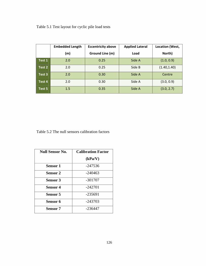
126
Table 5.1 Test layout for cyclic pile load tests
Embedded Length
(m)
Eccentricity above
Ground Line (m)
Applied Lateral
Load
Location (West,
North)
Test 1 2.0 0.25 Side A (1.0, 0.9)
Test 2 2.0 0.25 Side B (1.40,1.40)
Test 3 2.0 0.30 Side A Centre
Test 4 2.0 0.30 Side A (3.0, 0.9)
Test 5 1.5 0.35 Side A (3.0, 2.7)
Table 5.2 The null sensors calibration factors
Null Sensor No. Calibration Factor
(kPa/V)
Sensor 1 -247536
Sensor 2 -240463
Sensor 3 -301707
Sensor 4 -242701
Sensor 5 -235691
Sensor 6 -243703
Sensor 7 -236447
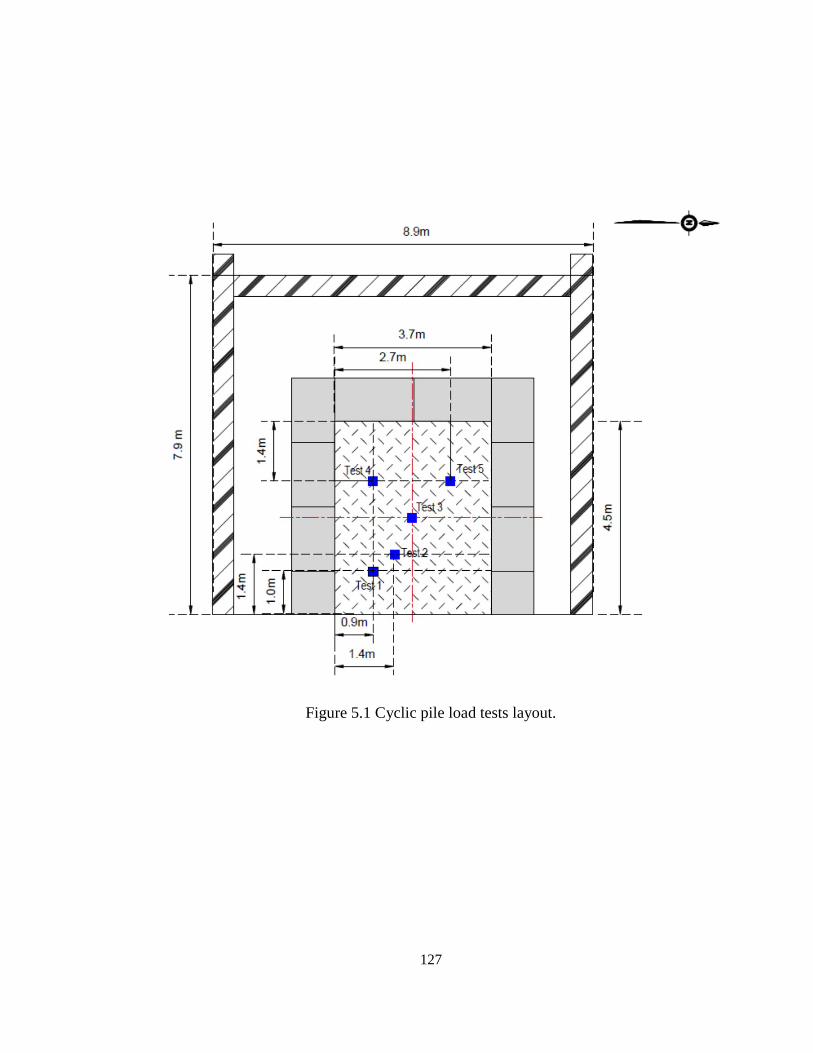
127
Figure 5.1 Cyclic pile load tests layout.
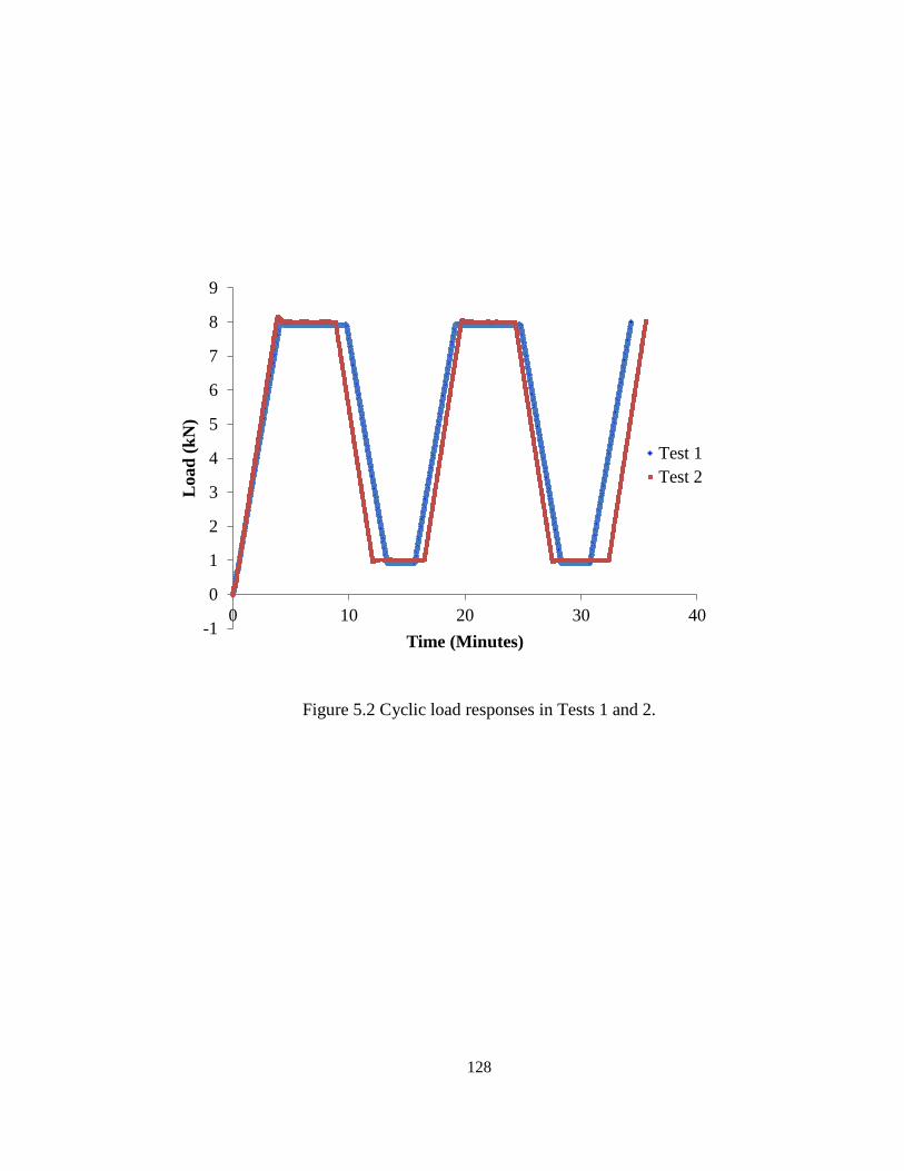
128
Figure 5.2 Cyclic load responses in Tests 1 and 2.
-1
0
1
2
3
4
5
6
7
8
9
0 10 20 30 40
Load
(k
N)
Time (Minutes)
Test 1
Test 2
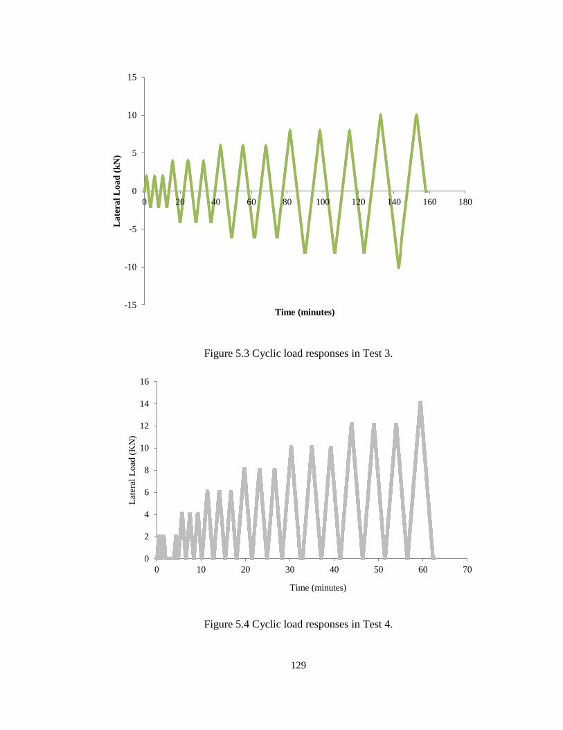
129
Figure 5.3 Cyclic load responses in Test 3.
Figure 5.4 Cyclic load responses in Test 4.
-15
-10
-5
0
5
10
15
0 20 40 60 80 100 120 140 160 180
La
tera
l L
oa
d (
kN
)
Time (minutes)
0
2
4
6
8
10
12
14
16
0 10 20 30 40 50 60 70
Lat
eral
Lo
ad (
KN
)
Time (minutes)
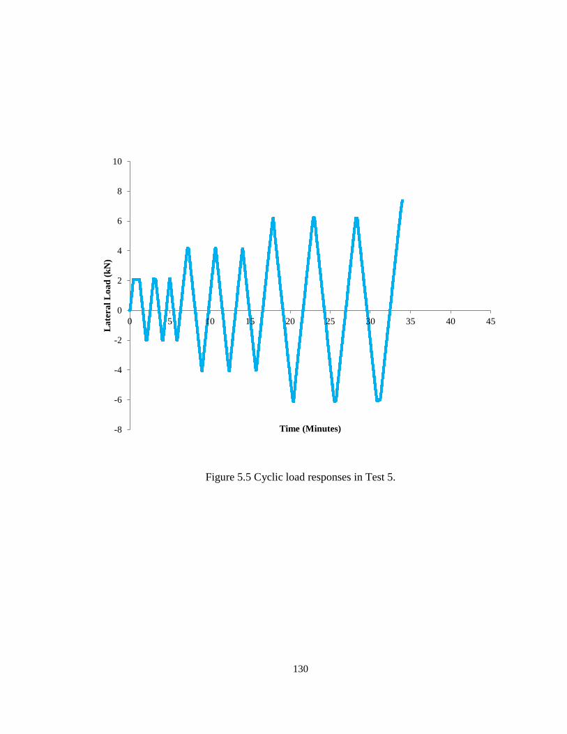
130
Figure 5.5 Cyclic load responses in Test 5.
-8
-6
-4
-2
0
2
4
6
8
10
0 5 10 15 20 25 30 35 40 45
La
tera
l L
oa
d (
kN
)
Time (Minutes)
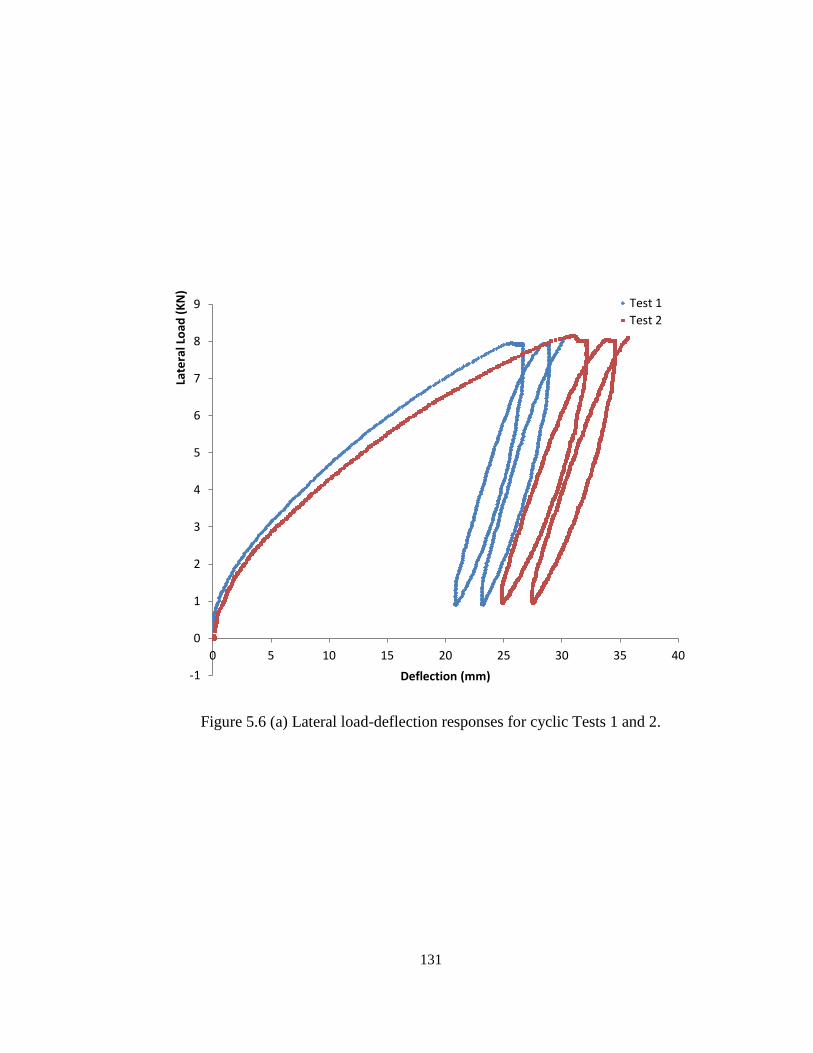
131
Figure 5.6 (a) Lateral load-deflection responses for cyclic Tests 1 and 2.
-1
0
1
2
3
4
5
6
7
8
9
0 5 10 15 20 25 30 35 40
Late
ral L
oad
(K
N)
Deflection (mm)
Test 1
Test 2
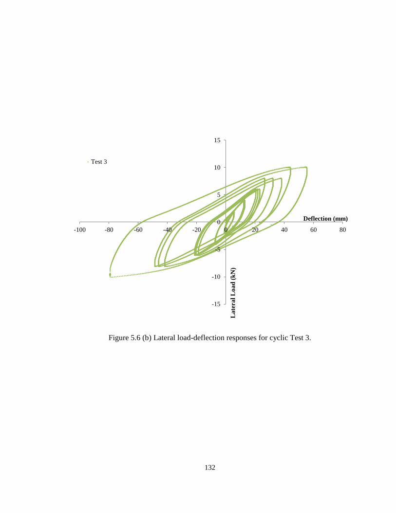
132
Figure 5.6 (b) Lateral load-deflection responses for cyclic Test 3.
-15
-10
-5
0
5
10
15
-100 -80 -60 -40 -20 0 20 40 60 80L
ate
ra
l L
oa
d (
kN
)
Deflection (mm)
Test 3
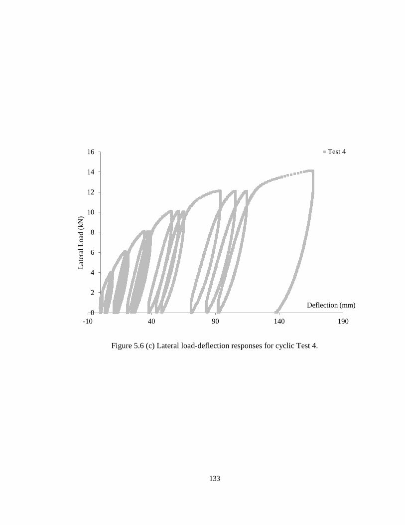
133
Figure 5.6 (c) Lateral load-deflection responses for cyclic Test 4.
0
2
4
6
8
10
12
14
16
-10 40 90 140 190
Lat
eral
Load
(kN
)
Deflection (mm)
Test 4
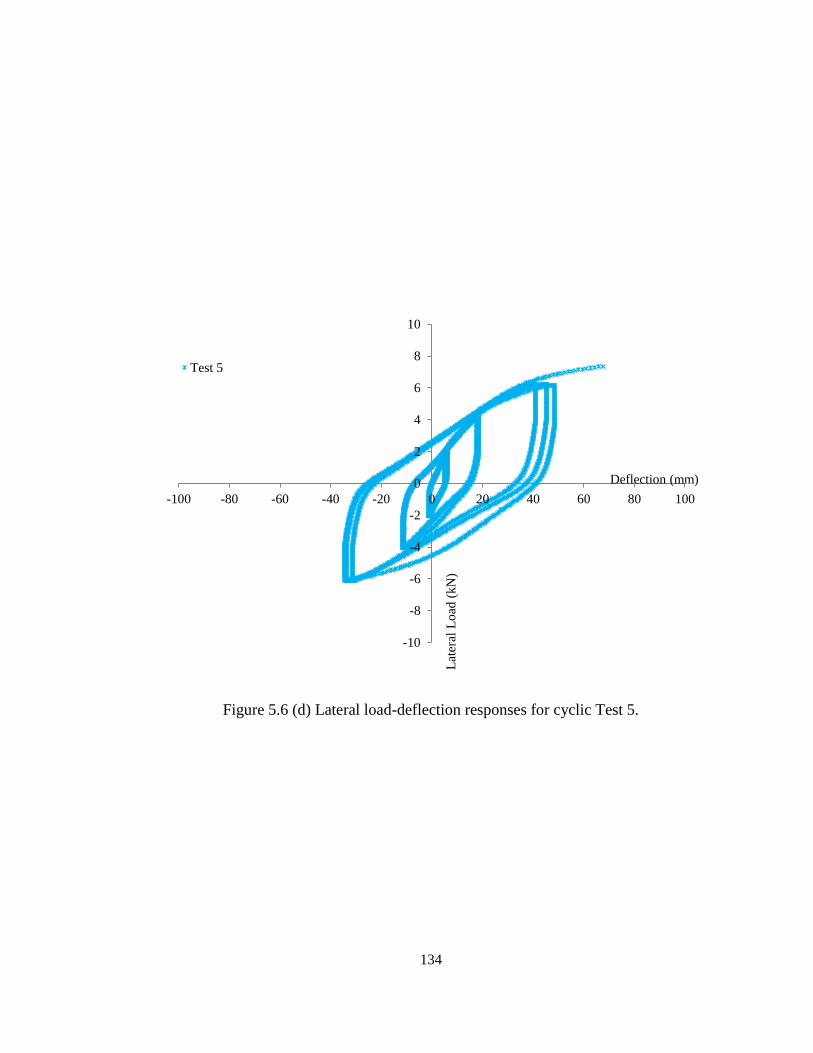
134
Figure 5.6 (d) Lateral load-deflection responses for cyclic Test 5.
-10
-8
-6
-4
-2
0
2
4
6
8
10
-100 -80 -60 -40 -20 0 20 40 60 80 100
Lat
eral
Lo
ad (
kN
)
Deflection (mm)
Test 5
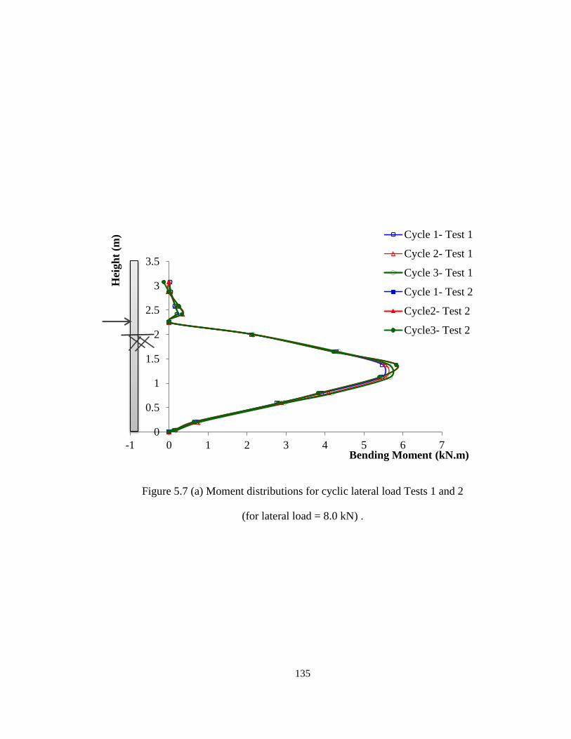
135
Figure 5.7 (a) Moment distributions for cyclic lateral load Tests 1 and 2
(for lateral load = 8.0 kN) .
0
0.5
1
1.5
2
2.5
3
3.5
-1 0 1 2 3 4 5 6 7
Hei
gh
t (m
)
Bending Moment (kN.m)
Cycle 1- Test 1
Cycle 2- Test 1
Cycle 3- Test 1
Cycle 1- Test 2
Cycle2- Test 2
Cycle3- Test 2
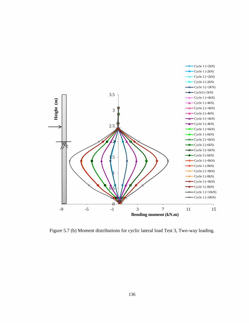
136
Figure 5.7 (b) Moment distributions for cyclic lateral load Test 3, Two-way loading.
0
0.5
1
1.5
2
2.5
3
3.5
-9 -5 -1 3 7 11 15
Hei
gh
t (
m)
Bending moment (kN.m)
Cycle 1 (+2kN)
Cycle 1 (-2kN)
Cycle 2 (+2kN)
Cycle 2 (-2kN)
Cycle 3 (+2KN)
Cycle3 (-2kN)
Cycle 1 (+4kN)
Cycle 1 (-4kN)
Cycle 2 (+4kN)
Cycle 2 (-4kN)
Cycle 3 (+4kN)
Cycle 3 (-4kN)
Cycle 1 (+6kN)
Cycle 1 (-6kN)
Cycle 2 (+6kN)
Cycle 2 (-6kN)
Cycle 3 (+6kN)
Cycle 3 (-6kN)
Cycle 1 (+8kN)
Cycle 1 (-8kN)
Cycle 2 (+8kN)
Cycle 2 (-8kN)
Cycle 3 (+8kN)
Cycle 3 (-8kN)
Cycle 1 (+10kN)
Cycle 1 (-10kN)
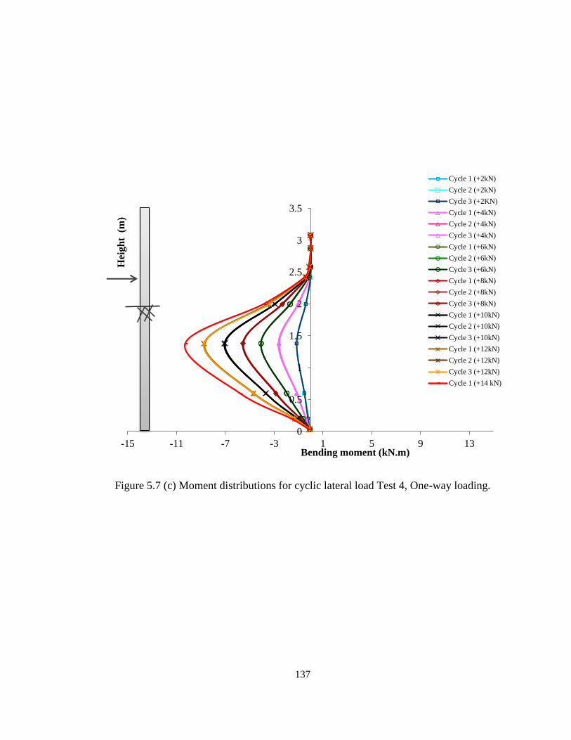
137
Figure 5.7 (c) Moment distributions for cyclic lateral load Test 4, One-way loading.
0
0.5
1
1.5
2
2.5
3
3.5
-15 -11 -7 -3 1 5 9 13
Hei
gh
t (
m)
Bending moment (kN.m)
Cycle 1 (+2kN)
Cycle 2 (+2kN)
Cycle 3 (+2KN)
Cycle 1 (+4kN)
Cycle 2 (+4kN)
Cycle 3 (+4kN)
Cycle 1 (+6kN)
Cycle 2 (+6kN)
Cycle 3 (+6kN)
Cycle 1 (+8kN)
Cycle 2 (+8kN)
Cycle 3 (+8kN)
Cycle 1 (+10kN)
Cycle 2 (+10kN)
Cycle 3 (+10kN)
Cycle 1 (+12kN)
Cycle 2 (+12kN)
Cycle 3 (+12kN)
Cycle 1 (+14 kN)
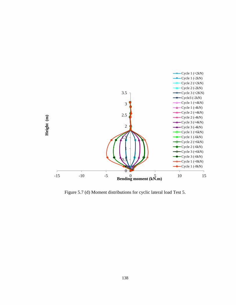
138
Figure 5.7 (d) Moment distributions for cyclic lateral load Test 5.
0
0.5
1
1.5
2
2.5
3
3.5
-15 -10 -5 0 5 10 15
Hei
gh
t (
m)
Bending moment (kN.m)
Cycle 1 (+2kN)
Cycle 1 (-2kN)
Cycle 2 (+2kN)
Cycle 2 (-2kN)
Cycle 3 (+2KN)
Cycle3 (-2kN)
Cycle 1 (+4kN)
Cycle 1 (-4kN)
Cycle 2 (+4kN)
Cycle 2 (-4kN)
Cycle 3 (+4kN)
Cycle 3 (-4kN)
Cycle 1 (+6kN)
Cycle 1 (-6kN)
Cycle 2 (+6kN)
Cycle 2 (-6kN)
Cycle 3 (+6kN)
Cycle 3 (-6kN)
Cycle 1 (+8kN)
Cycle 1 (-8kN)
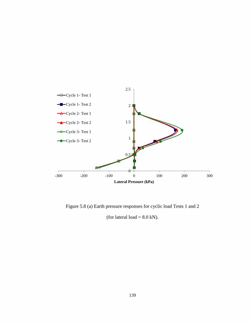
139
Figure 5.8 (a) Earth pressure responses for cyclic load Tests 1 and 2
(for lateral load = 8.0 kN).
0
0.5
1
1.5
2
2.5
-300 -200 -100 0 100 200 300
Lateral Pressure (kPa)
Cycle 1- Test 1
Cycle 1- Test 2
Cycle 2- Test 1
Cycle 2- Test 2
Cycle 3- Test 1
Cycle 3- Test 2
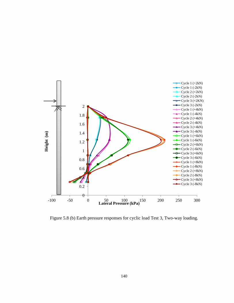
140
Figure 5.8 (b) Earth pressure responses for cyclic load Test 3, Two-way loading.
0
0.2
0.4
0.6
0.8
1
1.2
1.4
1.6
1.8
2
-100 -50 0 50 100 150 200 250 300
Hei
gh
t (
m)
Lateral Pressure (kPa)
Cycle 1 (+2kN)
Cycle 1 (-2kN)
Cycle 2 (+2kN)
Cycle 2 (-2kN)
Cycle 3 (+2KN)
Cycle 3 (-2kN)
Cycle 1 (+4kN)
Cycle 1 (-4kN)
Cycle 2 (+4kN)
Cycle 2 (-4kN)
Cycle 3 (+4kN)
Cycle 3 (-4kN)
Cycle 1 (+6kN)
Cycle 1 (-6kN)
Cycle 2 (+6kN)
Cycle 2 (-6kN)
Cycle 3 (+6kN)
Cycle 3 (-6kN)
Cycle 1 (+8kN)
Cycle 1 (-8kN)
Cycle 2 (+8kN)
Cycle 2 (-8kN)
Cycle 3 (+8kN)
Cycle 3 (-8kN)
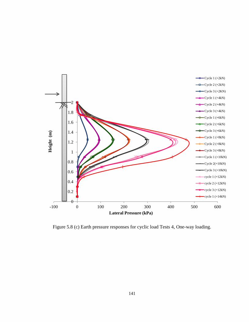
141
Figure 5.8 (c) Earth pressure responses for cyclic load Tests 4, One-way loading.
0
0.2
0.4
0.6
0.8
1
1.2
1.4
1.6
1.8
2
-100 0 100 200 300 400 500 600
Hei
gh
t (
m)
Lateral Pressure (kPa)
Cycle 1 (+2kN)
Cycle 2 (+2kN)
Cycle 3 (+2KN)
Cycle 1 (+4kN)
Cycle 2 (+4kN)
Cycle 3 (+4kN)
Cycle 1 (+6kN)
Cycle 2 (+6kN)
Cycle 3 (+6kN)
Cycle 1 (+8kN)
Cycle 2 (+8kN)
Cycle 3 (+8kN)
Cycle 1 (+10kN)
Cycle 2(+10kN)
Cycle 3 (+10kN)
cycle 1 (+12kN)
cycle 2 (+12kN)
cycle 3 (+12kN)
cycle 1 (+14kN)
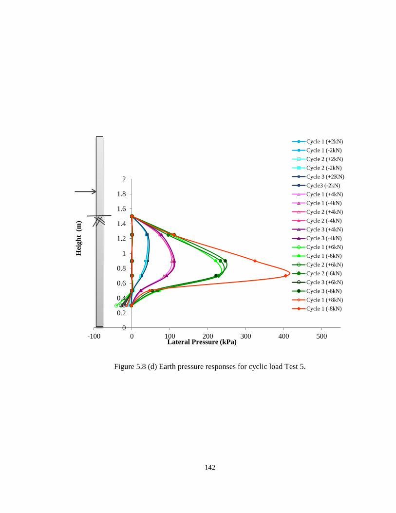
142
Figure 5.8 (d) Earth pressure responses for cyclic load Test 5.
0
0.2
0.4
0.6
0.8
1
1.2
1.4
1.6
1.8
2
-100 0 100 200 300 400 500
Hei
gh
t (
m)
Lateral Pressure (kPa)
Cycle 1 (+2kN)
Cycle 1 (-2kN)
Cycle 2 (+2kN)
Cycle 2 (-2kN)
Cycle 3 (+2KN)
Cycle3 (-2kN)
Cycle 1 (+4kN)
Cycle 1 (-4kN)
Cycle 2 (+4kN)
Cycle 2 (-4kN)
Cycle 3 (+4kN)
Cycle 3 (-4kN)
Cycle 1 (+6kN)
Cycle 1 (-6kN)
Cycle 2 (+6kN)
Cycle 2 (-6kN)
Cycle 3 (+6kN)
Cycle 3 (-6kN)
Cycle 1 (+8kN)
Cycle 1 (-8kN)
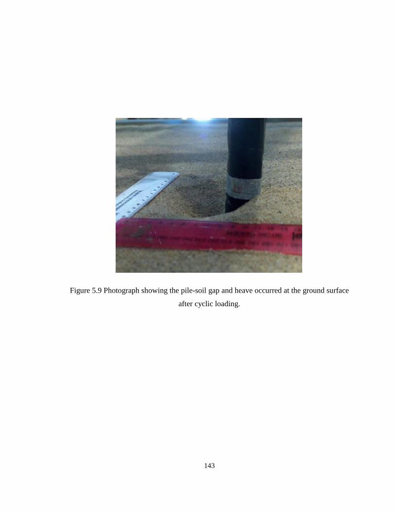
143
Figure 5.9 Photograph showing the pile-soil gap and heave occurred at the ground surface
after cyclic loading.
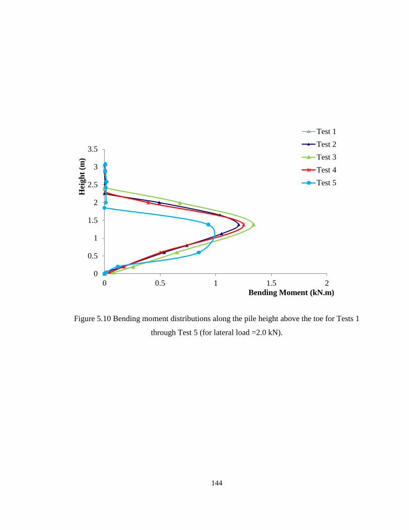
144
Figure 5.10 Bending moment distributions along the pile height above the toe for Tests 1
through Test 5 (for lateral load =2.0 kN).
0
0.5
1
1.5
2
2.5
3
3.5
0 0.5 1 1.5 2
Hei
gh
t (m
)
Bending Moment (kN.m)
Test 1
Test 2
Test 3
Test 4
Test 5
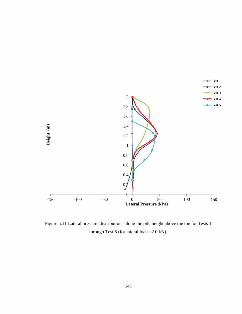
145
Figure 5.11 Lateral pressure distributions along the pile height above the toe for Tests 1
through Test 5 (for lateral load =2.0 kN).
0
0.2
0.4
0.6
0.8
1
1.2
1.4
1.6
1.8
2
-150 -100 -50 0 50 100 150
Hei
gh
t (
m)
Lateral Pressure (kPa)
Test1
Test 2
Test 3
Test 4
Test 5
146
Chapter 6
CONCLUSIONS AND RECOMMENDATIONS
6.1 CONCLUSIONS
Pile behaviour has been the subject of many studies but the novelty of the current study
involved the use of high quality measurements of lateral earth pressure from null sensors,
together with more conventional measurements of moment and deformation. The purpose
of this work was to understand experimental response of a pile in sand under static and
cyclic lateral loads. Therefore, pile load tests were performed on a fabricated pile which
was instrumented with axial strain gauges and null sensors. The pile installation and all
lateral load tests were conducted at the Geo-Engineering Laboratory at Queen's
University using large scale test facilities and dry Olivine Sand was used as the test soil.
This chapter summarises the main findings of this study and provides recommendations
for future research.
6.1.1 Bending Test Results
Prior to performing pile load tests, beam bending tests were conducted to confirm that all
the instrumentation was performing well and providing consistent readings. The results
confirmed that approximately zero pressure readings were obtained in the case of pile
bending when there was no contact pressures and the bending strains did not lead to
spurious readings. The other objective of bending tests was to find out the flexural
147
rigidity of the test pile. The flexural rigidity of the pile was estimated from measured
deflection and measured curvature from bending test results. The moment distributions
were calculated based on the flexural rigidities and compared to the moment from statics
A flexural rigidity of 1015 kN/m2
was selected for the test pile.
6.1.2 Axial Responses
The purpose of this thesis is to study static and cyclic responses of a pile under lateral
loading but since some axial responses were measured during pile insertion, the axial
load responses were presented briefly. The axial force distributions along the pile burial
depth illustrate that shear stresses up the sides of the pile provide most of the axial
resistance and the shaft resistance increased more rapidly near the ground surface than at
depth.
In addition, bending moment and normal contact pressure responses were measured at the
end of installation. The results show that the moment and lateral pressure that developed
during pile installation were less than 10% of those seen subsequently under lateral
loading.
6.1.3 Static Lateral Responses
The initial pile response under monotonically increasing lateral load was examined for
two tests. The peak lateral load for each test were kept below the ultimate lateral
capacity, estimated from theoretical lateral responses of the pile based on Broms'
148
methods (1964) to avoid pile yielding. The measured parameters in all pile load tests
were deflection, load, axial strain and lateral contact pressure.
Bending moment distributions were estimated from the measured strain readings at the
maximum applied load. In addition, load-deflection responses were examined to estimate
the stiffness of the soil. The deflection results show that soil stiffness decreases with
increase in lateral loading. Difference of less than 10% in maximum soil displacements
were recorded at the same horizontal force, which may be attributed to changes in soil
stiffness and density. However, the moments calculated from measured strains indicated
that evaluations of stresses are not affected by changes in soil characteristics or other test
conditions during the two repeated tests.
Another feature of the lateral responses of pile are the lateral soil pressures measured
along the pile shaft (Leland and Kraft, 1991). The lateral forces were calculated assuming
zero shear stress and uniform force distributed across the pile width. If the measured
pressures are assumed to act across the whole of the pile width, and a simple triangular
pressure distributions is employed, the result horizontal force was 94% of the value
applied by the actuator. This provides support for the pressure measurements, and also
suggests that pressure values measured by the sensors are acting across the whole of the
pile width. The lateral pressure responses featured significant lateral stresses acting on
the null sensors, with values reaching peak values of 160 kPa on the faces being pushed
into the soil. The lateral pressure distributions follow the same pattern of pressures
presented by Prasad and Chari (1999). However, the results cannot be numerically
compared with their existing design method since Prasad and Chari predicted the
149
variation of pressure distributions at the peak state but the lateral peak load in Tests 1 and
2 was not at the ultimate capacity.
At the end, the lateral pressure distribution was estimated from the moment distribution.
The results support the use in other experimental programs of moment distributions and
the Bernoulli Euler beam equations to determine lateral pressures of the pile.
6.1.4 Cyclic Lateral Responses
It is important to predict pile responses under cyclic loading in the design of offshore
constructions since most offshore structures and bridges are subjected to cyclic loading.
In this study, five sets of cyclic load tests were conducted in a dry sand to examine the
effects of embedment, load eccentricity and loading conditions on cyclic pile responses.
The deflection responses show how deflection increases with increase in lateral loading
and each additional load cycle. During cyclic loading, elastic or plastic shakedown is
observed at low load levels from the load-deflection responses, in which the incremental
deflection responses trace the same path during each cycle. However, accumulation of
plastic deformation was recorded at higher load levels. Since three sets of consecutive
cycles were conducted at each load level, it is unclear whether these responses at higher
load levels would eventually shake down or continue to incremental collapse at higher
cycle numbers.
The moment distributions were estimated from the maximum strain readings for each
cycle. Unlike deflection responses, the moment responses are consistent for repeated
150
cycles under a given load and are not significantly influenced by any changes in the
surrounding soil stiffness from its initial state.
In addition, the measurement of lateral earth pressure along the pile length was reported.
For two-way cyclic loading, the lateral earth pressure responses are different than those
associated with a classic passive pressure distribution. The results show that peak
pressure is observed near the ground level for low load levels, whereas the peak pressure
moves deeper towards the point of rotation as the magnitude of cyclic lateral load
increases. This behaviour is understood to result from elastic soil response at low load
levels and the progressive development of inelastic response at higher load levels during
two-way cyclic loading. However for one-way cyclic loading, the patterns of lateral
pressure responses are similar to classic passive pressure distributions and it is therefore
concluded that the soil response around the pile is less elastic. The results show that these
one-way lateral pressure distributions do not exhibit stress proportional to displacement
at low load levels, and the location of peak pressures for all the cycles is consistent.
Decrease in soil support near the ground surface was observed due to the gapping
phenomenon, and this caused the point of rotation to move deeper as the lateral loading
increased.
At the end of Chapter 5, bending moment and lateral pressure distributions for all five
cyclic tests were compared and the results demonstrated that the pile responses are
sensitive to changes in embedment and loading condition (i.e. one-way versus two-way
loading). However, the effect of changes in load eccentricity on moment and pressure
151
responses was small (peak moments changed by 3%, and the patterns of lateral earth
pressures down the pile were almost unaffected).
6.2 RECOMMENDATIONS FOR FUTURE RESEARCH
The laboratory experiments reported in this dissertation represent a useful first study on
the static and cyclic responses of a pile in sand using high quality measurements of lateral
earth pressure. The following recommendations are made regarding future studies to
continue this research:
Measurement of the base pressure using a null sensor would assist in estimation
of pressures and moments. In particular, this would assist in estimating the
magnitude of friction on the base plate as the base moves laterally through the
soil.
Tests in other foundation materials would be useful for describing the pile
responses in cohesive material using the same instruments.
Pile group effects should be investigated to further expand our understanding of
static and cyclic pile load behaviour.
Additional null sensors near the ground surface would be advisable to obtain a
more comprehensive distribution of lateral pressure and examine gapping effects
on pressure responses.
152
Interpretation of the test data could be enhanced through development of other
options for analysis of the lateral load tests, such as modification of the existing
design methods or use of finite element analysis.
6.3 REFERENCES
Leland, M. and Kraft, Jr., 1991, Performance of Axially Loaded Pipe Piles in Sand.
Journal of Geotechnical Engineering, Vol. 117, No. 2, pp. 272-296.
Talesnick, M., 2005. Measuring Soil Contact Pressure on a Solid Boundary and
Quantifying Soil Arching. Geotechnical Testing Journal, Vol. 28, No. 2, pp. 1-9.
153
Appendix A
AXIAL LOAD RESPONSES
Piles are always subjected to axial forces due to its weight as well as additional loads,
which are axially transferred to the pile through its shaft and base. Therefore, it is
important to examine pile responses under axial loading. The primary purpose of this
research was to study lateral capacity of the pile in sand. However, the behaviour of the
pile was monitored during installation using the data acquisition system and some axial
measurements were recorded. Therefore, the axial pile responses were explained briefly
earlier the dissertation and the results are presented in this Appendix.
Axial force distributions
The variation of axial force along the pile length was obtained from the strain gauge
measurements. The axial force distributions at the end of insertion for all the tests are
presented in Figures A.1 and A.2. The embedded length of the pile was 2 m for Tests 1
through 4 and 1.5 m for Test 5. The results for Tests 1 to 4 feature similar axial force
patterns. However for burial depth of 1.5 m used in Test 5, less resistance was mobilized
(see Figure A. 2). The axial force distributions show that maximum axial force was
observed near the ground surface and the applied load is mainly supported by shaft
resistance.
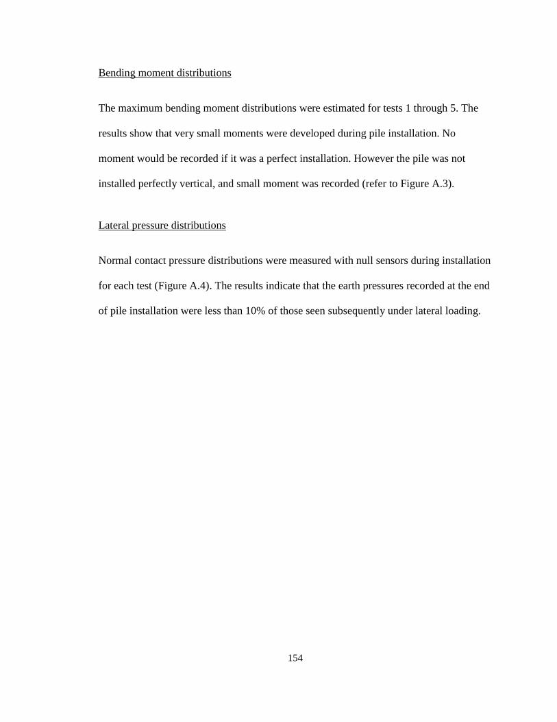
154
Bending moment distributions
The maximum bending moment distributions were estimated for tests 1 through 5. The
results show that very small moments were developed during pile installation. No
moment would be recorded if it was a perfect installation. However the pile was not
installed perfectly vertical, and small moment was recorded (refer to Figure A.3).
Lateral pressure distributions
Normal contact pressure distributions were measured with null sensors during installation
for each test (Figure A.4). The results indicate that the earth pressures recorded at the end
of pile installation were less than 10% of those seen subsequently under lateral loading.
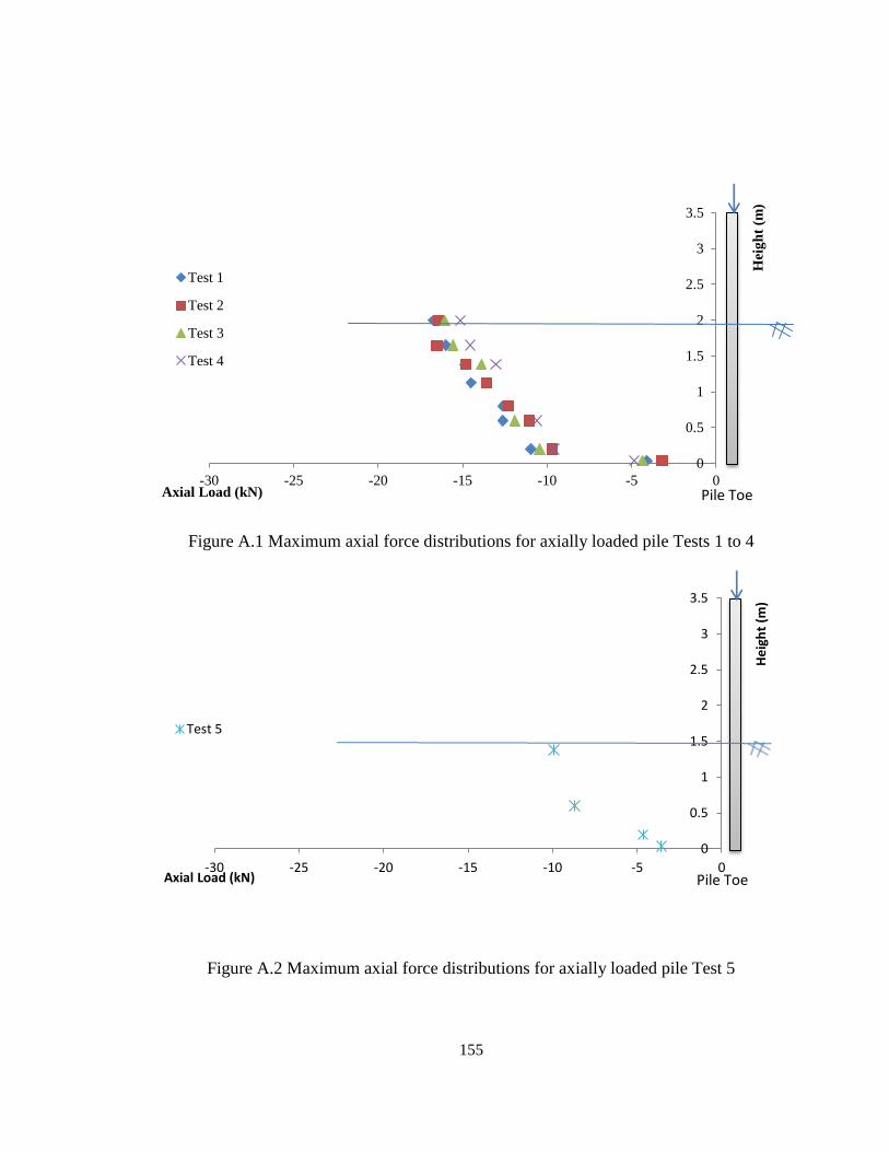
155
Figure A.1 Maximum axial force distributions for axially loaded pile Tests 1 to 4
Figure A.2 Maximum axial force distributions for axially loaded pile Test 5
0
0.5
1
1.5
2
2.5
3
3.5
-30 -25 -20 -15 -10 -5 0
Hei
gh
t (m
)
Axial Load (kN)
Test 1
Test 2
Test 3
Test 4
Pile Toe
0
0.5
1
1.5
2
2.5
3
3.5
-30 -25 -20 -15 -10 -5 0
He
igh
t (m
)
Axial Load (kN)
Test 5
Pile Toe
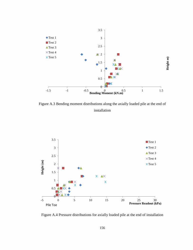
156
Figure A.3 Bending moment distributions along the axially loaded pile at the end of
installation
Figure A.4 Pressure distributions for axially loaded pile at the end of installation
0
0.5
1
1.5
2
2.5
3
3.5
-1.5 -1 -0.5 0 0.5 1 1.5
Hei
gh
t m
)
Bending Moment (kN.m)
Test 1
Test 2
Test 3
Test 4
Test 5
0
0.5
1
1.5
2
2.5
3
3.5
-5 0 5 10 15 20 25 30
Hei
gh
t (m
)
Pressure Readout (kPa)
Test 1
Test 2
Test 3
Test 4
Test 5
Pile Toe