3D failure envelope of a single pile in sand

HAL Id: hal-01235181https://hal.archives-ouvertes.fr/hal-01235181

Submitted on 1 Jul 2016

HAL is a multi-disciplinary open accessarchive for the deposit and dissemination of sci-entific research documents, whether they are pub-lished or not. The documents may come fromteaching and research institutions in France orabroad, or from public or private research centers.

L’archive ouverte pluridisciplinaire HAL, estdestinée au dépôt et à la diffusion de documentsscientifiques de niveau recherche, publiés ou non,émanant des établissements d’enseignement et derecherche français ou étrangers, des laboratoirespublics ou privés.

3D failure envelope of a single pile in sandZheng Li, Panagiotis Kotronis, Sandra Escoffier

To cite this version:Zheng Li, Panagiotis Kotronis, Sandra Escoffier. 3D failure envelope of a single pile in sand. COMP-DYN 2015, 5th ECCOMAS Thematic Conference on Computational Methods in Structural Dynamicsand Earthquake Engineering, May 2015, Crete Island, Greece. pp.2752-2760. �hal-01235181�

https://hal.archives-ouvertes.fr/hal-01235181

https://hal.archives-ouvertes.fr

COMPDYN 20155th ECCOMAS Thematic Conference on

Computational Methods in Structural Dynamics and Earthquake EngineeringM. Papadrakakis, V. Papadopoulos, V. Plevris (eds.)

Crete Island, Greece, 25–27 May 2015

3D FAILURE ENVELOPE OF A SINGLE PILE IN SAND

Zheng Li1,2, Panagiotis KOTRONIS1 and Sandra ESCOFFIER2

1LUNAM Universite, Ecole Centrale de Nantes, Universite de Nantes, CNRSInstitut de Recherche en Genie Civil et Mecanique (GeM)

1 Rue de la Noe, F-44321 Nantes, Francee-mail: {zheng.li,Panagiotis.Kotronis}@ec-nantes.fr

2 LUNAM Universite, IFSTTAR, GERS, SVF-44341 Bouguenais, France

e-mail: [email protected]

Keywords: Pile, Foundation, Capacity diagram, Sand, Failure envelope.

Abstract. Pile foundations are widely used in geotechnical and offshore engineering. Whensubjected to a combination of horizontal, vertical forces and bending moments, a 3D failureenvelope is necessary in order to evaluate the safety of the pile-soil system. We present a studyon the failure envelope of a single elastic pile in sand. In order to find it in the three-dimensionalspace (i.e. horizontal force H, bending moment M and vertical force V), the radial displacementmethod and swipe tests are numerically performed. An analytical equation providing goodagreement with the 3D numerical results is finally proposed.

Z. LI, P. KOTRONIS and S. ESCOFFIER

1 INTRODUCTION

The failure envelope of a single elastic vertical pile in sand is numerically investigated viaswipe tests and a large number of radial displacement controlled tests. The analytical equationproposed by Meyerhof [1] is validated and adopted in the H-V plane. For the H-M-V spacehowever, a new 3D analytical failure envelope is introduced. The proposed failure envelope isuseful for the development of new simplified modelling strategies for soil-structure interactionproblems (e.g. macro-elements [2]) that can be applied in design engineering offices [3].

2 NUMERICAL MODEL

2.1 SOIL CONSTITUTIVE LAW

A hypoplastic constitutive law, similar to an elastic perfectly plastic Drucker-Prager model,is used to numerically reproduce the behaviour of a single pile in sand. The basic frameworkof the hypoplastic formulation is provided with the following equations (bold letters definehereafter tensors and vectors, the dot“ ˙ ” symbol is the derivative with respect to time and ‖‖the norm of a tensor):

T = LD+N‖D‖ (1)

where T and D are the stress rate and stretching rate tensors. The stiffness matrix L dependson the bulk modulus K and the shear modulus in the elastic range Gmax and has the followingform (the Lame coefficient µ = Gmax according to Hooke’s law):

L = K1⊗ 1 + 2µ

[I− 1

31⊗ 1

](2)

The constitutive tensor N is defined following the approach proposed by Niemunis [4]:

N(T) = −y(T)Lm(T) (3)

where y(T) is a scalar function that controls the variation of the nonlinear term and m(T)defines the plastic flow direction. The scalar function 0 ≤ y(T) ≤ 1 is chosen as a function ofthe current stress q(T) =

√3J2 and a predefined limit stress σy(T) as follows:

y(T) =

(q(T)

σy(T)

)nc

(4)

with nc is a constant that controls the isotropic evolution of y(T) and J2 the second invariantof the deviatoric stress tensor. Assuming a dry sand and thus a zero cohesive strength (c = 0),kc = 0 and the yield function reads:

F = q(T)−Mc p(T) = 0 (5)

The plastic flow direction m(T) is defined according to the bounding surface model [5, 6, 7]and it is given by Eq. 6:

m(T) =∂G/∂T

‖∂G/∂T‖(6)


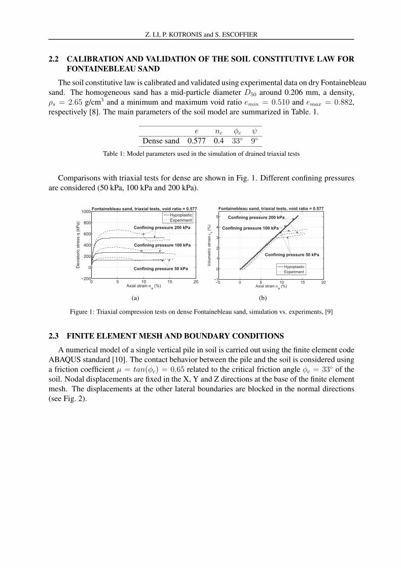
2.2 CALIBRATION AND VALIDATION OF THE SOIL CONSTITUTIVE LAW FORFONTAINEBLEAU SAND

The soil constitutive law is calibrated and validated using experimental data on dry Fontainebleausand. The homogeneous sand has a mid-particle diameter D50 around 0.206 mm, a density,ρs = 2.65 g/cm3 and a minimum and maximum void ratio emin = 0.510 and emax = 0.882,respectively [8]. The main parameters of the soil model are summarized in Table. 1.

e nc φc ψDense sand 0.577 0.4 33◦ 9◦

Table 1: Model parameters used in the simulation of drained triaxial tests

Comparisons with triaxial tests for dense are shown in Fig. 1. Different confining pressuresare considered (50 kPa, 100 kPa and 200 kPa).

0 5 10 15 20−200

0

200

400

600

800

1000

Axial strain σa (%)

Dev

iato

ric s

tress

q (k

Pa)

HypoplasticExperiment

Fontainebleau sand, triaxial tests, void ratio = 0.577

Confining pressure 100 kPa



(a)

−5 0 5 10 15 20−1

0

1

2

3

4

5

Axial strain σa (%)

Vol

umet

ric s

trrai

n ε v (%

)

HypoplasticExperiment




Fontainebleau sand, triaxial tests, void ratio = 0.577

(b)

Figure 1: Triaxial compression tests on dense Fontainebleau sand, simulation vs. experiments, [9]

2.3 FINITE ELEMENT MESH AND BOUNDARY CONDITIONS

A numerical model of a single vertical pile in soil is carried out using the finite element codeABAQUS standard [10]. The contact behavior between the pile and the soil is considered usinga friction coefficient µ = tan(φc) = 0.65 related to the critical friction angle φc = 33◦ of thesoil. Nodal displacements are fixed in the X, Y and Z directions at the base of the finite elementmesh. The displacements at the other lateral boundaries are blocked in the normal directions(see Fig. 2).


X

Y

Z

10D

20D

23.1 D

16.64 m

XZ

XY

Figure 2: Finite element model for a single vertical pile in soil

3 NUMERICAL STUDY OF THE 3D FAILURE ENVELOPE

3.1 PARAMETERS OF THE FINITE ELEMENT MODEL

In the finite element model, the pile has a length of 13 m, a diameter of 0.72 m, a slendernessratio of 18 and the pile head is considered on the ground surface level. Poulos and Davis[11] proposed a method to classify piles in different categories based on a flexibility factor.According to this method, the pile is classified as flexible.

3.2 3D NUMERICAL FAILURE ENVELOPE

In order to numerically reproduce the 3D failure envelope, the radial displacement test pro-posed by Gottardi et al. [12] is adopted. The sign conventions for the pile head loads (horizontalforce, vertical force and bending moment) are presented in Fig. 3.

Forces Moments

X

Y

Resultant force

Figure 3: Sign conventions for the pile head loadings

3.2.1 NUMERICAL FAILURE ENVELOPE IN THE H-V PLANE

To investigate the form of the failure surface in the H-V plane, free pile head conditions(M=0) are considered. A displacement is applied on the top of the pile head (that can rotatefreely) in a certain direction δ. The angle of the displacement δ varies from 0 ∼ 360◦ to scanthe failure surface in all directions. The final strength is chosen as the point where numerical cal-culation diverges. By connecting the values at the ends of the different load paths the completefailure surface is thus obtained. Examples of load paths in the H-V plane from the numerical


radial displacement tests are shown in Fig. 5(a). Numerical swipe tests are also performed inH-V plane, Fig. 5(b) and for more complex loads in Fig. 5(c). A large number (around 500) ofnumerical radial displacement tests are performed and the ultimate strength (or failure locus) ofeach test is plotted in Fig. 5(d).

Sandδ

Direction of imposeddisplacement

X

Y

Figure 4: Radial displacements tests in the H-V plane

−1 −0.5 0 0.5 1

x 104

−0.5

0

0.5

1

1.5

2

2.5

3x 10

4

Horizontal force (kN)

Ver

tical

forc

e (k

N)

Load paths

(a)

−1 −0.5 0 0.5 1

x 104

−0.5

0

0.5

1

1.5

2

2.5

3x 10

4


Ver

tical

forc

e (k

N)

Load paths

(b)

−1 −0.5 0 0.5 1

x 104

−0.5

0

0.5

1

1.5

2

2.5

3x 10

4


Ver

tica

l fo

rce

(kN

)

Load path 01Load path 02

(c)

−1 −0.5 0 0.5 1

x 104

−0.5

0

0.5

1

1.5

2

2.5

3x 10

4


Ver

tical

forc

e (k

N)

(d)

Figure 5: Selected load paths from numerical radial displacement tests (a), load paths from numerical swipetests (b), numerical swipe tests with more complex load paths (c) and complete results from numerical radialdisplacement test (d), in H-V plane (M=0), [9].

3.2.2 NUMERICAL FAILURE ENVELOPE IN THE H-M PLANE

The failure envelope is hereafter investigated in the H-M plane and for different verticalloading levels. First, the pile is loaded until a certain vertical force. Then, radial displacementloadings are applied considering a constant ratio between the combined rotation-displacementsincrements. Similar to the H-V plane, load paths in the H-M plane start from the origin andstop at the failure envelope, see Fig. 6(a). Results of the numerical radial displacement tests areprovided in Fig. 6(b).


−1.5 −1 −0.5 0 0.5 1 1.5

x 104

−1

−0.5

0

0.5

1x 10

5


Ben

ding

mom

ent (

kN*m

)

Load paths

(a)

−1.5 −1 −0.5 0 0.5 1 1.5

x 104

−1

−0.5

0

0.5

1x 10

5


Ben

ding

mom

ent (

kN*m

)

2

1

3

A

B

(b)

Figure 6: (a) Load paths (b) numerical radial displacement tests in the H-M plane corresponding to V=0, [9]

3.2.3 NUMERICAL FAILURE ENVELOPE IN THE H-M-V 3D SPACE

By combining the results in the H-V plane and in the H-M plane for different vertical loadlevels, the complete failure envelope is plotted in Fig. 7.

−2

−1

0

1

2

x 104

−2−101234−1

−0.5

0

0.5

1

Horizontal force (kN)Vertical force (kN)

Bending moment (kN*m)

x 104

x 105

Figure 7: Numerical failure envelope in the H-M-V 3D space, [9]

From the numerical radial tests in Fig. 7 the horizontal bearing capacity (V=0 and M=0)is estimated at H0 =5000 kN, the vertical compression bearing capacity (H=0 and M=0)Vc0 =25000 kN, the vertical tension bearing capacity (H=0 and M=0) Vt0 = 5100 kN andthe ultimate bending resistance (H=0 and V=0) M0 = 0.42×105 kN·m.

3.3 ANALYTICAL EQUATIONS

3.3.1 ANALYTICAL EQUATION FOR THE FAILURE ENVELOPE IN THE H-V PLANE

Meyerhof and Ranjan [1] proposed a semi-empirical formula to evaluate the interaction be-tween the horizontal and vertical forces that reads:(

H

H0

)2

+

(V

V0

)2

= 1 (7)

where H0 and V0 are the horizontal and vertical bearing capacities of the pile. Eq. (7) can bewritten in a normalized form as follows:

f = m2 + υ2 − 1 (8)


where m = H/H0 and υ = V/Vc0 in compression or υ = V/Vt0 in tension. m and υ aredimensionless quantities. The comparison of the semi-empirical Eq. (8) with the numericalresults is shown in Fig. 8 (a) and (b). The agreement is satisfactory although some discrepanciesare identified in the tension part (dash line).

−1 −0.5 0 0.5 1

x 104

−0.5

0

0.5

1

1.5

2

2.5

3x 10

4


Ver

tical

forc

e (k

N)

Data pointsEmpirical equation

(a)

−1 −0.5 0 0.5 1−1.5

−1

−0.5

0

0.5

1

1.5

Normalized horizontal force, H/H0

Nor

mal

ized

ver

tical

forc

e, V

/Vc0

, V/V

t0

Data pointsEmpirical equation

HH0

VVc0

VVt0

(b)

Figure 8: Comparison of Eq. (8) with the numerical results (a) in the H-V plane and (b) in the normalized HH0

- VVc0

- VVt0

space, [9]

3.3.2 ANALYTICAL EQUATION FOR THE FAILURE ENVELOPE IN THE H-M-V3D SPACE

As shown in section 3.2.2, the failure envelope in the H-M plane has an inclined ellipticalshape. Inspired from the work of Gottardi et al. [12], a similar equation is proposed hereafterfor a single pile in sand:

f = αm2 + ξn2 − βmn− ρ(υ) = 0 (9)

where m = H/H0 the normalized horizontal force, n = M/M0 the normalized bending mo-ment and υ = V/Vc0 or υ = V/Vt0 the normalized vertical force (dependent on the sign of thevertical load). α, ξ, β and ρ are constants that control the shape of the ellipse. The parametersare first fitted using the normalized numerical data in the H-M plane at zero vertical force. Theyare found equal to α = 1.0, ξ = 1.0, β = 1.5 and ρ = 1.0, Eq. (9) thus becomes:

f = 1.0m2 + 1.0n2 − 1.5mn− 1.0 = 0 (10)

The fitted curves are plotted in Fig. 9 (a) and (b) and show a good agreement with the numericaldata both in the H-M and in the normalized H/H0 - M/M0 plane.


−1 −0.5 0 0.5 1

x 104

−8

−6

−4

−2

0

2

4

6

8x 10

4


Ben

ding

mom

ent (

kN*m

)

(a)

−2 −1 0 1 2

−2

−1

0

1

2

Normalized Horizontal force, H/H0

Nor

mal

ized

Mom

ent,

M/M

0

(b)

Figure 9: Comparison of Eq. (10) with the numerical results (a) in the H-M plane and (b) in the normalized HH0

-MM0

plane, [9]

The vertical load influences the size of the elliptical cross-sections but not their inclinations.In order to introduce this behaviour, it is proposed hereafter to link the parameter ρ in Eq. (9)and Eq. (10) with the vertical load as follows:

f = 1.0m2 + 1.0n2 − 1.5mn− (1− υ2) = 0 (11)

The 3D failure envelope for a single vertical pile in sand defined by Eq. (11) is plotted inFig. 10 together with all the numerical data points.

−1

0

1x 104

−1 −0.5 0 0.5 1 1.5 2 2.5 3x 104

−8

−6

−4

−2

0

2

4

6

8

x 105

Horizontal force (kN)Vertical force (kN)

Bending moment (kN*m)

Data points

H

M

V

Figure 10: 3D failure envelope for a single vertical pile in sand: yield surface provided by Eq. (11) Vs. numericaldata points, [9]

4 CONCLUSIONS

This paper presents a numerical study on the 3D failure envelope of a single elastic pile insand and analytical equations are proposed. The key parameters for the analytical equations arerelatively easy to determine either experimentally or numerically making the above equationsuseful for engineering design offices. More details on this work can be found in [9], [13]and [14].


REFERENCES

[1] G. G. Meyerhof and G. Ranjan. The bearing capacity of rigid piles under inclined loadsin sand. I: Vertical piles. Canadian Geotechnical Journal, 9(4):430–446., 1972.

[2] S. Grange, P. Kotronis, and J. Mazars. A macro-element to simulate 3D soil-structure in-teraction considering plasticity and uplift. International Journal of Solids and Structures,46(20):3651 – 3663, 2009.

[3] S. Grange, L. Botrugno, P. Kotronis, and C. Tamagnini. The effects of soil-structureinteraction on a reinforced concrete viaduct. Earthquake Engineering and Structural Dy-namics, 40(1):93–105, 2011.

[4] Andrzej Niemunis. Extended hypoplastic models Dissertation submitted for habilitation.Habilitation thesis, Ruhr-University, Bochum, 2002.

[5] Y. F. Dafalias. Bounding surface plasticity. I: Mathematical foundation and hypoplasticity.Journal of Engineering Mechanics, 112(9):966–987, 1986.

[6] Y.F. Dafalias and L.R. Herrmann. Bounding surface formulation of plasticity. John Wileyand Sons, Ltd., 1982.

[7] J. P. Bardet. Bounding surface plasticity model for sands. Journal of engineering mechan-ics, 112(11):1198–1217., 1986.

[8] I. Andria-Ntoanina, J. Canou, and J. C. Dupla. Caracterisation mecanique du sable deFontainebleau NE34 a lappareil triaxial sous cisaillement monotone. Technical report,Laboratoire Navier - Geotechnique (CERMES, ENPC/LCPC), 2010.

[9] Z. Li, P. Kotronis, and S. Escoffier. Numerical study of the 3D failure envelope of a singlepile in sand. Computers and Geotechnics, 62:11–26, 2014.

[10] Abaqus/Standard. Abaqus 6.10 Documentation (SIMULIA Abaqus 6.10). DassaultSystemes, 2010.

[11] H. G. Poulos and E. H. Davis. Pile foundation analysis and design. John Wiley and Sons,Inc., New York, 1980.

[12] G Gottardi, G.T. Houlsby, and R. Butterfield. Plastic response of circular footings on sandunder general planar loading. Geotechnique, 49(4):453–469, 1999.

[13] Z. Li, S. Escoffier, and P. Kotronis. Using centrifuge tests data to identify the dynamic soilproperties: application to Fontainebleau sand. Soil Dynamics and Earthquake Engineer-ing, 52:77–87, September 2013.

[14] Z. Li, P. Kotronis, S. Escoffier, and C. Tamagnini. A hypoplastic macroelement for singlevertical piles in sand subject to threedimensional loading conditions. Earthquake Engi-neering and Structural Dynamics (submitted), 2015.

Documents

3D failure envelope of a single pile in sand