ANALYTICAL EVALUATION OF VOLATILITY FORECASTS

INTERNATIONAL ECONOMIC REVIEWVol. 45, No. 4, November 2004

ANALYTICAL EVALUATION OF VOLATILITY FORECASTS∗

BY TORBEN G. ANDERSEN, TIM BOLLERSLEV, AND NOUR MEDDAHI1

Northwestern University and National Bureau of Economic Research;Duke University and National Bureau of Economic Research;

Universite de Montreal (CIRANO, CIREQ), Canada

Estimation and forecasting for realistic continuous-time stochastic volatilitymodels is hampered by the lack of closed-form expressions for the likelihood. Inresponse, Andersen, Bollerslev, Diebold, and Labys (Econometrica, 71 (2003),579–625) advocate forecasting integrated volatility via reduced-form models forthe realized volatility, constructed by summing high-frequency squared returns.Building on the eigenfunction stochastic volatility models, we present analyticalexpressions for the forecast efficiency associated with this reduced-form approachas a function of sampling frequency. For popular models like GARCH, multi-factor affine, and lognormal diffusions, the reduced form procedures performremarkably well relative to the optimal (infeasible) forecasts.

1. INTRODUCTION

Continuous-time stochastic volatility models figure prominently in modernasset-pricing theories. At the same time, empirical analysis of such models are gen-erally complicated by intractable expressions for the likelihood of the observeddiscrete-time returns. Even though a burst of research activity has brought impor-tant advances (see, e.g., the surveys in Aıt-Sahalia et al., 2005; Gallant and Tauchen,2005; and Johannes and Polson, 2005), the discrete-time (G)ARCH class of mod-els remains the workhorse for modeling and forecasting time-varying volatilityin situations of practical import. However, recent developments in economet-ric methodology and the increasing availability of richer data sources hold thepromise of a paradigm shift.

∗ Manuscript received October 2002; revised June 2003.1 This work was supported by a grant from the National Science Foundation to the NBER (Andersen

and Bollerslev), and from FQRSC, IFM2, MITACS, NSERC, SSHRC, and Jean-Marie Dufour’sEconometrics Chair of Canada (Meddahi). Discussions with Francis X. Diebold on closely relatedideas have been very helpful. We would also like to thank seminar audiences at Universite de Montreal,University of Pennsylvania, the Federal Reserve Board, the NSF/NBER Time Series Conference 2002,Philladelphia, the CIRANO-CIREQ Conference on Extremal Events in Finance, the 2003 WesternFinance Association Meeting, Rob Engle, Rossen Valkanov, and especially Neil Shephard for helpfulcomments on the first version of the article. Comments from the editor and two anonymous refer-ees also greatly improved the exposition. The third author thanks the Bendheim Center for Finance,Princeton University, for its hospitality during his visit and the revision of the article. Please addresscorrespondence to: Torben G. Andersen, Kellogg Graduate School of Management, NorthwesternUniversity, 2001 Sheridan Road, Evanston, IL 60208-2001. Phone: 847-467-1285. Fax: 847-491-5719.E-mail: [email protected].

1079

1080 ANDERSEN, BOLLERSLEV, AND MEDDAHI

In particular, from the perspectives of asset pricing and risk management, in-terest typically centers on (forecasts for) the integrated volatility as opposed to thepoint-in-time (spot) volatility, which often serves as a (latent) state variable in theformulation of continuous-time models. Moreover, from a statistical perspective,the integrated volatility provides a direct measure of the discrete-time return vari-ability appropriately defined (see, e.g., the discussion in Andersen et al., 2005 andAndersen, Bollerslev, Diebold, and Labys, 2003, henceforth ABDL). These ob-servations, along with the increased availability of continuously recorded intradayprices (ultra-high-frequency data in the terminology of Engle, 2000), have spurredmuch recent research into the measurement, modeling, and forecasting of inte-grated volatility based on discretely sampled realized volatilities constructed fromthe summation of finely sampled squared high-frequency returns (e.g., Andersenand Bollerslev, 1998; Comte and Renault, 1998; ABDL, 2001, 2003; Barndorff-Nielsen and Shephard, 2001, 2002a,b; Meddahi, 2002).

Specifically, the empirical results of ABDL (2003) suggest that relatively simplediscrete-time ARMA-based forecasts for realized volatility compare admirably toforecasts based on standard volatility models employed within the academic liter-ature and among practitioners. Of course, from a statistical perspective these easy-to-compute reduced-form time series forecast for the observed realized volatilitiesinvariably entail a loss in efficiency relative to the optimal, but generally infea-sible, forecasts for the latent integrated volatilities based on the true underlyingcontinuous-time model.

In response to this, the present article provides explicit analytical expressions forthe expected future integrated volatility for the most popular stochastic volatilitydiffusion models employed in the literature, including GARCH, multifactor affine,and lognormal diffusions. We obtain these results by exploiting the general findingsfor the eigenfunction stochastic volatility model class introduced by Meddahi(2001). By conditioning the expectations on the full sample path realization of thelatent volatility process,2 as well as the coarser information set consisting of onlythe lagged realized volatilities constructed from the high-frequency returns overfixed-length time intervals, our results allow for a direct assessment of the trade-off between modeling complexity, sampling frequency, and forecast accuracy. Assuch, it also directly quantifies the loss associated with simple feasible proceduresrelative to the optimal, but infeasible ones.3

Following Andersen and Bollerslev (1998) and ABDL (2003) among others,we focus our forecast comparisons on the value of the coefficient of multiple cor-relation in the ex post regressions of the (latent) integrated volatility of interestson the forecasts obtained from the different volatility modeling procedures.4 On

2 Throughout the article, we identify the path realization of the volatility process and the pathrealization of the state variable driving the volatility process. We will be more specific when thedifference between these two paths is important for forecasting purposes.

3 This type of analysis parallels previous studies related to the predictability of mean asset returns;see, e.g., the discussion in Campbell et al. (2004).

4 No universally acceptable loss function exists for the evaluation of nonlinear model forecasts; see,e.g., the discussion in Andersen et al. (1999) and Christoffersen and Diebold (2000). The particular lossfunction used here is directly inspired by the earlier contributions of Mincer and Zarnowitz (1969),

EVALUATION OF VOLATILITY FORECASTS 1081

numerically quantifying this loss for empirically realistic sampling frequencies forseveral specific models recently reported in the literature, we find that the simplediscrete-time autoregressive models for the realized volatilities perform remark-ably well compared to the fully efficient (nonfeasible) continuous-time modelforecasts conditional on the full sample-path realization of the latent volatilityprocess. Hence, our results lend additional theoretical support to the use of sim-ple empirical reduced-form modeling and forecasting procedures based on theobservable realized volatilities in situations of practical import.

The plan for the rest of the article is as follows. The next section formally definesthe notions of integrated and realized volatility within the class of continuous-timestochastic volatility models. We also briefly review the arguments for focusing onforecasts of integrated volatility based on projections involving realized volatility.Section 3 introduces the eigenfunction stochastic volatility class of models un-derlying our theoretical derivations, and also sets out the three specific modelsthat form the basis for our numerical calculations. Section 4 presents analyticalexpressions for the optimal (nonfeasible) one- and multi-step-ahead forecasts forthe integrated volatility conditional on the full sample path realization of the la-tent spot volatility process, along with the less efficient (still nonfeasible) forecastsconditional on the coarser information set consisting of “only” the lagged inte-grated volatilities. Section 5 in turn presents the (feasible) forecasts for the futureintegrated volatilities conditional on the past observable realized volatilities. Thissection also quantifies the corresponding loss in efficiency for each of the three il-lustrative candidate models as a function of the sampling frequency of the returnsused in the construction of the realized volatilities. Section 6 concludes. All proofsare relegated to the Appendix.

2. INTEGRATED AND REALIZED VOLATILITY

We focus on a single asset traded in a liquid financial market. Assuming thesample path of the corresponding price process, {St, 0 ≤ t}, to be continuous,5

the class of continuous-time stochastic volatility models traditionally employed inthe finance literature is conveniently expressed in terms of the following genericstochastic differential equation (SDE):

d log(St ) = µt dt + σt dWt(1)

where Wt denotes a standard Brownian motion, the volatility term σ t is pre-dictable, and the drift term µt is predictable and of finite variation.6 The

and we will refer to the corresponding regression as such; see also the discussion in Chong and Hendry(1986).

5 The discussion in this section explicitly rules out discontinuities in the price process. However,our new theoretical results based on the eigenfunction stochastic volatility class of models could fairlyeasily be extended to allow for jumps. We briefly allude to this possibility in Section 3.

6 The drift, µt , may generally depend explicitly on both St and σ t . However, we suppressed all thearguments for notational simplicity.


point-in-time, or spot, volatility process {σ t , 0 ≤ t} measures the instantaneousstrength of the price variability expressed per unit of time.

Following standard practice we assume that the sample path of the σ t processis also continuous. Generally, σ t and Wt may be contemporaneously correlated,so that a so-called leverage style effect is allowed. However, the (asymptotic)distributional result discussed in this section is only known to be true under theassumption that dσ t and dWt are uncorrelated (no leverage effect). Likewise, theresults concerning realized volatility in Section 5 preclude leverage effects. In con-trast, the new theoretical results in Sections 3 and 4 explicitly allow for a nonzero(instantaneous) correlation, and we conjecture that the key results on realizedvolatility in Section 5 will be (approximately) valid in this case as well. Likewise,to facilitate the exposition, we explicitly exclude jump processes although manyof the results remain valid for empirically relevant jump specifications.

The SDE in Equation (1) greatly facilitates arbitrage-based pricing arguments.However, as emphasized by Andersen et al. (2005), practical return calculationsand volatility measurements are invariably restricted to discrete time intervals. Inparticular, focusing on the unit time interval, the one-period continuously com-pounded return corresponding to (1) is formally given by

rt ≡ log(St ) − log(St−1) =∫ t

t−1µu du +

∫ t

t−1σu dWu(2)

Hence, with no leverage effect and conditional on the sample-path realizationsof the drift and volatility processes, {µu, t − 1 ≤ u ≤ t} and {σ u, t − 1 ≤ u ≤ t},the one-period returns will be Gaussian with conditional mean equal to the firstintegral on the right-hand side of Equation (2), whereas the conditional varianceequals the integrated volatility

IVt ≡∫ t

t−1σ 2

u du(3)

The integrated volatility, therefore, affords a natural measure of the (ex post)return variability, as recently highlighted in independent work by Andersen andBollerslev (1998), Comte and Renault (1998), and Barndorff-Nielsen and Shep-hard (2001). The integrated volatility also plays a key role in the stochastic volatil-ity option pricing literature. In particular, ignoring the variation in the conditionalmean, Hull and White (1987) show that option prices are uniquely determined bythe expected future integrated volatility (see also Garcia et al. 2001).

Of course, integrated volatility is not directly observable. This has spurred thedevelopment of several new statistical procedures for modeling and forecastingthe (latent) integrated volatility based on specific parametric models within thegeneral diffusion class of models in Equation (1) (see, e.g., Gallant et al., 1999;Barndorff-Nielsen and Shephard, 2001; and the references therein). Althoughthese procedures allow for the construction of asymptotically optimal forecastsunder appropriate conditions, they are generally not robust to misspecifications ofthe underlying continuous-time model, and also quite complicated to implement.


Alternatively, consider the so-called realized volatility defined by the summationof intraperiod squared returns

RVt (h) ≡1/h∑i=1

r (h)2t−1+ih(4)

where the h-period return is given by r (h)t = log(St) − log(St−h) and 1/h is a pos-

itive integer. By the theory of quadratic variation, RVt(h) converges uniformlyin probability to IVt as h → 0, thus allowing for increasingly more accuratenonparametric measurements of integrated volatility as the sampling frequencyof the underlying intraperiod returns increases.

If we further assume that the realized and integrated volatility measures aresquare integrable, the asymptotic unbiasedness of RVt(h) for IVt, implies thatforecasts for IVt+ j , j ≥ 1, based on the projection of RVt+ j (h) on any time tinformation set, will also be (asymptotically) unbiased and optimal in a meansquare error (MSE) sense relative to that particular information set.7 In particular,restricting the information set to the lagged realized volatilities only, as proposedby ABDL (2003), conveniently circumvents the complications associated with theuse of latent variable procedures in the construction of the integrated volatilityforecasts. Of course, doing so also entails a loss in forecast efficiency relativeto the optimal (nonfeasible) forecasts for IVt+ j conditional on the full samplepath realization of the instantaneous price and (latent) spot volatility processes.However, as we show below, this loss in efficiency is typically fairly small. We nextturn to a discussion of the eigenfunction stochastic volatility class of models usedin our formal derivation of this important practical result.

3. EIGENFUNCTION STOCHASTIC VOLATILITY MODELS

This section reviews the main properties of the eigenfunction stochastic volatil-ity (ESV) models introduced in Meddahi (2001) and provides a discussion of thespecific parametric models considered in our numerical calculations. The ESVclass of models includes most continuous-time stochastic volatility models ana-lyzed in the existing literature. Meanwhile, the formulation in terms of orthogonaleigenfunctions provides a particular convenient and elegant framework for thederivation of explicit analytical expressions for volatility forecasts.

3.1. General Theory. The generic stochastic volatility model in Equation (1)is only restricted by the requirement that the point-in-time, or spot, volatility

7 This result holds generally subject to a uniform integrability condition ensuring convergencein expectation of the uniformly consistent realized volatility measure. As such, it includes cases inwhich the continuous sample path assumption for spot volatility is violated; see, e.g., the discussionin Andersen et al. (2005) and Barndorff-Nielsen and Shephard (2002b). Hoffman-Jørgensen (1994,Sections 3.22–3.25) provides a formal discussion of the necessary uniform integrability conditions onthe underlying price process to ensure convergence in expectation. See also Billingsley (1986, Exercise21.21) for the identical result.


process, σ t , be nonnegative (and continuous). Most popular stochastic volatilitymodels in the existing literature are based on the additional assumptions that thevolatility process is driven by a single (latent) state variable. In the context of theESV class of models, the corresponding one-factor representation takes the form

d log(St ) = µt dt + σt[√

1 − ρ2dW(1)t + ρdW(2)

t

](5)

where W(1)t and W(2)

t denote two independent standard Brownian motions, andthe instantaneous volatility is related to the latent state variable

dft = m( ft ) dt +√

v( ft ) dW(2)t(6)

by the functional relationship

σ 2t =

p∑i=0

ai Pi ( ft )(7)

where the integer p may be infinite, the ai coefficients are real numbers, thePi( f t)s denote the eigenfunctions of the infinitesimal generator associated withf t, with corresponding eigenvalues (−λi ), and the normalizations P0( f t) = 1 andVar[Pi( f t)] = 1 for i = 0 are imposed for notational simplicity.8

The expression for σ 2t in Equation (7) may appear somewhat arbitrary. Impor-

tantly, however, any square-integrable function g( f t) can be written as a linearcombination of the eigenfunctions associated with f t, i.e.,

g( ft ) =∞∑

i=0

ai Pi ( ft )(8)

where ai = E[g( f t)Pi( f t)] and∑∞

i=0 a2i = E[g( ft )2] < ∞, so that g( f t) is the

limit in mean square of∑p

i=0 ai Pi ( ft ) for p going to infinity. As such, the ESVstructure encompasses the popular GARCH diffusion model (Nelson, 1990), aswell as the lognormal model (Hull and White, 1987; Wiggins, 1987) and the square-root model of Heston (1993); these examples are considered in the followingsubsection.

The power of the ESV representations of these and other continuous-timestochastic volatility models essentially stems from the following two properties.First, the eigenfunctions associated with different eigenvalues are orthogonal andany nonconstant eigenfunction is centered at zero (for i , j > 0 and i = j):

E[Pi ( ft )Pj ( ft )] = 0 and E[Pi ( ft )] = 0(9)

8 For a more detailed discussion of the properties of infinitesimal generators see, e.g., Hansen andScheinkman (1995) and Aıt-Sahalia et al. (2005).


These features, of course, underlie the result noted after Equation (8) that∑∞i=0 a2

i = E[g( ft )2]. Second, the eigenfunctions are first-order autoregressiveprocesses (in general heteroskedastic):

∀l > 0, E[Pi ( ft+l) | fτ , τ ≤ t] = exp(−λi l)Pi ( ft )(10)

Given the structure of the ESV model and the Markovian nature of the jointprocess (St, f t), conditional expectations of any transformation of this variable,including the variance, therefore, only depend on the expectations of the eigen-functions. The orthogonality of the eigenfunctions coupled with the simple first-order autoregressive dynamics in turn render such calculations straightforward.

The ESV representations discussed above are based on a single (latent) statevariable. Meanwhile, several recent studies, including Alizadeh et al. (2002),Bollerslev and Zhou (2002), Engle and Lee (1999), Gallant et al. (1999), andHarvey et al. (1994), among others, have argued for the empirical relevance of al-lowing for multiple volatility factors. Fortunately, the ESV approach easily allowsfor multiple factors, while maintaining the validity of the formulas in (8), (9), and(10); see Meddahi (2001) for further details.9

3.2. Specific Illustrations. The numerical analysis presented in subsequentsections is based on three specific models, namely, a GARCH diffusion model,a two-factor affine model, and a lognormal diffusion. Meddahi (2001) shows howeach of these models may be represented as an ESV model by explicitly solving forthe corresponding eigenfunctions. The following subsections provide a brief sum-mary of these results along with the actual parameter values used in the numericalcalculations.

3.2.1. Model M1—GARCH diffusion. The instantaneous volatility in theGARCH diffusion model is defined by the process

dσ 2t = κ

(θ − σ 2

t

)dt + σσ 2

t dW(2)t

This model was first introduced by Wong (1964) and later popularized by Nelson(1990). The model is readily expressed as an ESV model by defining the statevariable

dft = κ(θ − ft ) dt + σ ft dW(2)t

and the function g(x) = x. Assuming that the variance of σ 2t is finite, it is possible

to show that

σ 2t = a0 + a1 P1( ft )

9 See also Chen et al. (2000) for a general approach to eigenfunction modeling for multivariateMarkov processes.


where a0 = θ , a1 = θ√

ψ/(1 − ψ), ψ = σ 2/2κ , and the first eigenfunction for f t isaffine

P1(x) =√

1 − ψ

θ√

ψ(x − θ)

with corresponding eigenvalue λ1 = κ . As discussed above, this representationof the process greatly facilitates any expected variance and/or volatility forecastcalculations. Note also that the second moment of the variance σ 2

t is assured tobe finite for ψ less than 1. In the numerical calculations reported here we rely onthe parameters from Andersen and Bollerslev (1998) as implied from the (weak)daily GARCH(1,1) model estimates for the DM/dollar from 1987 through 1992using the temporal aggregation results of Drost and Nijman (1993) and Drost andWerker (1996). In particular, κ = 0.035, θ = 0.636, and ψ = 0.296. These parametervalues were also used in the studies by Andersen et al. (1999) and Andreou andGhysels (2002).

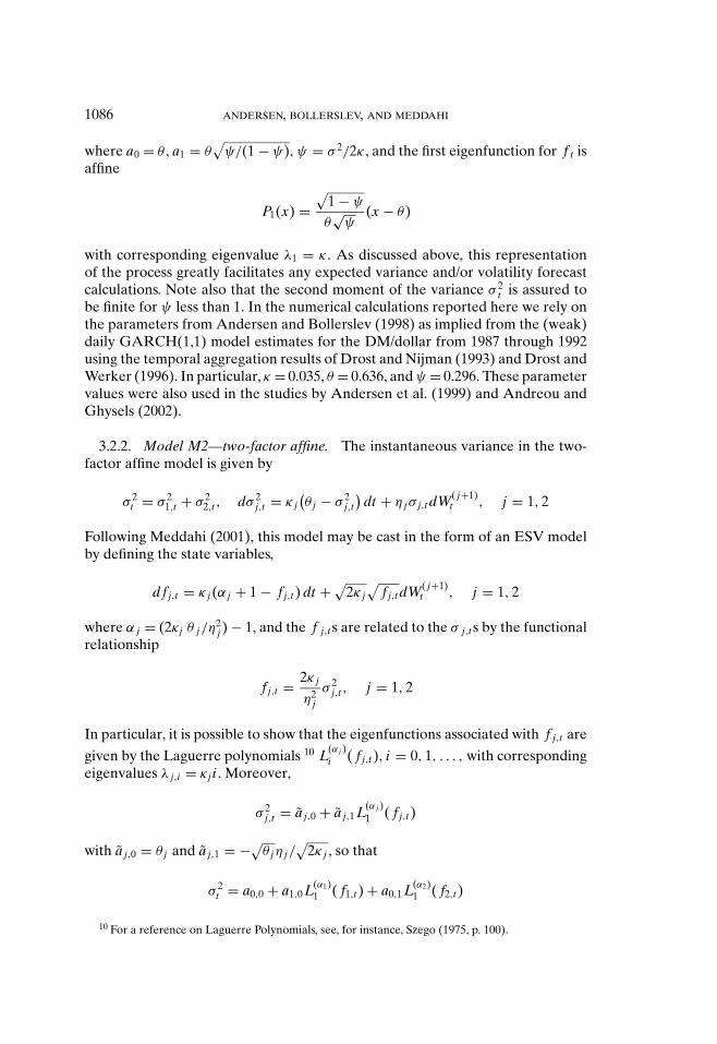
3.2.2. Model M2—two-factor affine. The instantaneous variance in the two-factor affine model is given by

σ 2t = σ 2

1,t + σ 22,t , dσ 2

j,t = κ j(θ j − σ 2

j,t

)dt + η jσ j,t dW( j+1)

t , j = 1, 2

Following Meddahi (2001), this model may be cast in the form of an ESV modelby defining the state variables,

df j,t = κ j (α j + 1 − f j,t ) dt + √2κ j

√f j,t dW( j+1)

t , j = 1, 2

where α j = (2κj θ j/η2j ) − 1, and the f j,t s are related to the σ j,t s by the functional

relationship

f j,t = 2κ j

η2j

σ 2j,t , j = 1, 2

In particular, it is possible to show that the eigenfunctions associated with f j,t are

given by the Laguerre polynomials 10 L(α j )i ( f j,t ), i = 0, 1, . . . , with corresponding

eigenvalues λ j,i = κj i . Moreover,

σ 2j,t = a j,0 + a j,1L(α j )

1 ( f j,t )

with a j,0 = θ j and a j,1 = −√θ jη j/

√2κ j , so that

σ 2t = a0,0 + a1,0L(α1)

1 ( f1,t ) + a0,1L(α2)1 ( f2,t )

10 For a reference on Laguerre Polynomials, see, for instance, Szego (1975, p. 100).


where a0,0 = a1,0 + a2,0, a1,0 = a1,1, and a0,1 = a2,1. The actual numerical results forthe two-factor model are based on the parameter estimates reported in Bollerslevand Zhou (2002) obtained by matching the sample moments of the daily realizedvolatilities constructed from high-frequency 5-minute DM/dollar returns spanning1986 through 1996 to the corresponding population moments for the integratedvolatility. The resulting values are κ1 = 0.5708, θ1 = 0.3257, η1 = 0.2286, κ2 =0.0757, θ2 = 0.1786, and η2 = 0.1096, implying the existence of a very volatile firstfactor, along with a much more slowly mean-reverting second factor.

3.2.3. Model M3—lognormal diffusion. Our last numerical example is basedon the lognormal diffusion model

d log(σ 2

t

) = κ[θ − log

(σ 2

t

)]dt + σdW(2)

t

Again, following Meddahi (2001), this model may be expressed in the form of anESV model by defining the state variable

dft = −κ ft dt +√

2κdW(2)t

related to σ t by the functional relationship

ft =√

2κ

σ

(log σ 2

t − θ)

The eigenfunctions associated with this Ornstein–Uhlenbeck process for f t aregiven by the usual Hermite polynomials Hi( f t), i = 0, 1, . . . , with correspondingeigenvalues λi = κi . Hence

σ 2t =

∞∑i=0

ai Hi ( ft )

where the ai coefficients take the form

ai = exp(

θ + σ 2

4κ

)(σ/

√2κ)i

√i!

Our numerical illustrations for this model rely on the EMM-based parame-ter estimates for the daily S&P500 returns spanning 1953 through 1996 re-ported in Andersen et al. (2002), where we restrict the estimated correlationbetween dW(1)

t and dW(2)t related to the leverage effect to be zero. In particular,

κ = 0.0136, θ = −0.8382, and σ = 0.1148. Finally, the summation in (7) is truncatedat p = 100.


4. IDEAL INTEGRATED VOLATILITY FORECASTS

This section provides analytic expressions for the basic dependency structureof integrated volatility across the full range of ESV diffusion models. Building onthese findings, we go on to characterize the extent of the predictability of inte-grated volatility for any member of this important class of asset price processes.The predictability is obviously dependent on the assumed information set. Wepresent results ranging from the ideal case of knowing the current (latent) volatil-ity state, through knowing the spot volatility, to observing the past sequence ofintegrated volatility only. All such information sets are unattainable in practice,as they contain variables that are not observed, but rather must be estimated orextracted from discrete return data. Nonetheless, they serve as important bench-marks that establish the maximal predictability and reveal, step by step, how muchforecast power is lost as we condition on successively less informative, but em-pirically more readily approximated, variables. The results based on conditioningthe forecasts on past integrated volatility set the stage for the analysis of the feasi-ble integrated volatility forecasts based on realized volatility measures extracteddirectly from observed high-frequency, intraday data in the following section.

Our first proposition characterizes the basic first and second moment propertiesof the spot and integrated volatility processes within the ESV diffusion class (theproofs are given in the Appendix). The results are all new at this level of gener-ality, but some expressions are clearly related to the abstract characterization ofthe second moment properties of integrated volatility in Barndorff-Nielsen andShephard (2002a). Moreover, these authors also provide some concrete resultsfor special cases of the ESV model and the non-Gaussian Ornstein–Uhlenbeckmodel.

The natural “realized” benchmark for the multi-step-ahead forecasts at horizonn is given by the corresponding integrated volatility

IVt+1:t+n =n∑

i=1

IVt+i(11)

PROPOSITION 1. For any ESV diffusion model, as defined in Section 3.1 (withpotential nonzero drift or leverage effects), and any integers n ≥ 1, l ≥ 0, we have

E[σ 2

t

] = a0, E[IVt+1:t+n] = na0(12)

E[σ 2

t+n

∣∣ Sτ , fτ , τ ≤ t] = a0 +

p∑i=1

ai exp(−λi n)Pi ( ft )(13)

E[IVt+1:t+n | Sτ , fτ , τ ≤ t] = na0 +p∑

i=1

ai[1 − exp(−λi n)]

λiPi ( ft )(14)

Var[σ 2

t

] =p∑

i=1

a2i , Var[IVt+1:t+n] = 2

p∑i=1

a2i

λ2i

[exp(−λi n) + λi n − 1](15)


Cov(IVt+1:t+n, σ

2t−l

) =p∑

i=1

a2i

[1 − exp(−λi n)]λi

exp(−λi l)(16)

Cov(IVt+1:t+n, IVt−l) =p∑

i=1

a2i

[1 − exp(−λi )][1 − exp(−λi n)]λ2

i

exp(−λi l)(17)

Cov(σ 2

t+n, σ2t

) =p∑

i=1

a2i exp(−λi n)(18)

One set of novel implications is given by the following corollary to Proposition 1.It provides a rather intuitive, yet useful, ranking of the second moment expressionsfor the different latent volatility notions.

PROPOSITION 2. Under the assumptions of Proposition 1, and ∀n ≥ 1, we have

Cov(σ 2

t+n, σ2t

) ≤ Cov(IVt+n, IVt ) ≤ Cov(IVt+n, σ

2t

) ≤ Var[IVt ] ≤ Var[σ 2

t

](19)

The inequalities are most readily understood by recalling the timing betweenspot and integrated volatility and recognizing that integrated volatility is asmoothed version of the spot volatility process. The first inequality, for exam-ple, reflects the fact that the spot volatilities are separated by n periods, whereasthe gap between the intervals over which the integrated volatilities, IVt+n and IVt,are measured is only n − 1 periods. The second inequality suggests that the spotvolatility at the interval end is more informative about future integrated volatilitythan the smoothed (average) spot volatility over the corresponding interval. Sucha conclusion appears natural in the single eigenfunction case, given the Markovstructure of ESV models, but is less obvious for the multiple eigenfunction casewhere affine functions of spot volatility cannot provide a sufficient statistic forthe volatility state vector, f t. The final inequalities are hardly surprising, but haveimportant implications. The variability of either volatility measure exceeds thecovariability measures and the smoothed integrated volatility measure is less vari-able than the spot volatility. The latter finding implies that the comparatively highcovariance between spot volatility and future integrated volatility may be dueto (excess) variability of spot volatility rather than superior correlation betweenspot and future (integrated) volatility. Hence, as discussed below, it is not clear ingeneral whether conditioning on the spot or the integrated volatility will allow forthe more efficient forecast.

4.1. Optimal One-Period-Ahead Forecasts. We are now in position to assessthe optimal integrated volatility forecasts generated by different information sets.We adopt the standard expected quadratic loss function, implying that optimalforecasts equal the conditional expectation of integrated volatility given the avail-able information. The universally best forecast is based on the full history of thelog-price and volatility path, denoted by the sigma algebra, σ (Sτ , f τ , τ ≤ t). Asdiscussed above, given the Markov structure of the ESV models, knowledge of


the state vector, f t, is sufficient for the construction of the optimal predictor.The coefficient of multiple correlation, or R2, from the Mincer–Zarnowitz typeregression of future integrated volatility on the corresponding (conditional ex-pectation) forecasts (and a constant) serves as a popular and useful summarymeasure of forecast performance. Moreover, it is consistent with the emphasison quadratic loss. For notational convenience, we focus our analysis on the one-period-ahead integrated volatility, IVt+1, but similar results are readily availablefor the n-period-ahead measure, IVt+n.

Proposition 1 and the orthogonality of the eigenfunctions, indicated in (9), implythat the “explained variation” from regressing IVt+1 onto E[IVt+1 | Sτ , f τ , τ ≤ t](and a constant), denoted R2(IVt+1, Best), is given by

R2(IVt+1, Best) = 1Var[IVt ]

p∑i=1

a2i

[1 − exp(−λi )]2

λ2i

(20)

with Var[IVt] determined by (15) (for n = 1).Alternatively, consider forecasts based on the current spot volatility. In one-

factor ESV models, there is no difference between the conditional expectationof integrated volatility given either spot volatility or the volatility state vector,so the two forecasts coincide. In multifactor models, however, the spot volatil-ity is not a sufficient statistic for the volatility state vector, with the latter be-ing more informative. Moreover, the process (St, σ t ) is not Markovian, and,hence, the associated optimal forecast—the conditional expectation of IVt+1 givenσ (Sτ , σ 2

τ , τ ≤ t)—depends in general on the entire path of σ 2t and is not available

in closed form.Consequently, we next consider a simple forecast that depends linearly on

σ 2t . Obviously, the best affine forecast of IVt+1 is given by the corresponding

(population) regression coefficients on σ 2t and a constant. Using (16), it follows

readily that the R2 of the corresponding Mincer–Zarnowitz regression, denotedR2(IVt+1, σ 2

t ), may be expressed as

R2(IVt+1, σ2t

) = 1Var[IVt ]Var

[σ 2

t

](

p∑i=1

a2i

[1 − exp(−λi )]λi

)2

(21)

where Var[IVt] and Var[σ 2t ] are given by (15). In the univariate factor case, if the

variance is solely a function of a single (nonconstant) eigenfunction, this forecaststill coincides with the “best.” However, when the variance depends on multipleeigenfunctions, the forecast will differ from the “best,” even in the case of a singlefactor. In the specific examples discussed in Section 3.2, we have one case (theGARCH diffusion) where the forecasts coincide (single factor, one eigenfunc-tion), one where they differ in a univariate factor model (the lognormal diffu-sion, where the variance depends on multiple eigenfunctions), and one where thespot volatility forecast is necessarily inferior to the “best”(the two-factors affinediffusion).


Forecasts based on integrated volatility are of particular interest as they, in prac-tice, may be approximated by the corresponding realized volatility obtained fromhigh-frequency data. Current (and past) integrated volatility will generally notprovide a sufficient statistic for the volatility state vector, so the optimal forecastsare not available in closed form and we again restrict attention to forecasts gen-erated by affine functions of the integrated volatility. In particular, on using (17)it follows that the R2 from the regression of IVt+1 on IVt and a constant, denotedR2(IVt+1, IVt), takes the form

R2(IVt+1, IVt ) =(

p∑i=1

a2i [1 − exp(−λi )]2/λ2

i

)2/Var[IVt ]2(22)

Obviously, the optimal forecast for the one-period integrated volatility will,by construction, dominate in terms of the population R2 from the associatedMincer–Zarnowitz regressions. More interesting is the relative performance ofthe forecasts in (21) and (22). Assuming a unique eigenfunction in (7), it followsthat11

R2(IVt+1, IVt ) ≤ R2(IVt+1, σ2t

)However, no general ranking of R2(IVt+1, IVt) relative to R2(IVt+1, σ 2

t ) is feasiblefor the case of multiple eigenfunctions.12 Intuitively, low persistence of the eigen-functions hurts the relative performance of integrated volatility based forecasts,whereas the main culprit behind poor performance of spot volatility-based predic-tors is a large discrepancy in persistence across the eigenfunctions (and associatedhigh variability of the spot volatility process). Interestingly, in spite of the highercovariance between the spot volatility and the future (integrated) volatility, it isgenerally not the case that the corresponding forecasts dominate those generatedby conditioning on the integrated volatility. In fact, this is only assured when thereis a single eigenfunction—in which case the spot volatility-based predictor coin-cides with the optimal one.13 In this situation, the integrated volatility forecastsshould ideally be based on (an estimate of) current spot volatility or (an estimateof) a current integrated volatility measure covering as short an intraday intervalas possible. However, practical difficulties in obtaining precise intraday-horizonvolatility estimates limit the applicability of this insight.

Indeed, from a practical perspective the more relevant question is how muchpredictive power is lost for the different forecasts and how one may alleviatethe loss in forecast accuracy if only historical integrated volatility-based predic-tors are feasible. We return to the first question in our numerical comparisons

11 By Equations (21), (22), and (15), the ratio R2(IVt+1, IVt)/R2(IVt+1, σ 2t ) equals (1 − exp(−λ1))2/

2(exp(−λ1) + λ1 − 1)), which necessarily is smaller than 1 by Equation (A.12) in the Appendix.12 For instance, consider the two numerical examples: p = 2, a1 = √

0.9, a2 = √0.1, λ1 = 0.002, and

λ2 = 4 in the first, and λ2 = 1 in the second. The ratio R2(IVt+1, IVt)/R2(IVt+1, σ 2t ) then equals 1.023

and 0.977, respectively.13 As noted above, the GARCH diffusion model falls in this category.


in Section 4.3. One approach for addressing the second question involves the in-clusion of additional (lagged) explanatory variables, as discussed formally in thefollowing section.

4.2. Multiple Explanatory Variables and Multiperiod Forecasts. Since the op-timal forecast of IVt+1 conditional on the history of spot volatility generally de-pends on the entire volatility path, it is natural to extend the expression for thebest affine forecast of IVt+1 given σ 2

t to include a fixed, finite number of laggedspot volatilities (and a constant) as regressors. Similarly, it is relevant to considerthe best affine forecast of IVt+1 given IVt and its lagged values.

For this purpose, it is convenient first to introduce some notation. For acovariance-stationary random variable (yτ , zt) and an integer l, we let C(yτ , zt, l)denote the (l + 1) vector defined by

C(yτ , zt , l) = (Cov[yτ , zt ], Cov[yτ , zt−1], . . . , Cov[yτ , zt−l])�(23)

Moreover, let M(zt, l) denote the (l + 1) × (l + 1) matrix whose (i, j)th componentis given by

M(zt , l)[i, j] = Cov[zt , zt+i− j ](24)

The R2 from the regression of IVt+1 onto a constant and (σ 2t , σ 2

t−1, . . . , σ 2t−l),

l ≥ 0, denoted R2(IVt+1, σ 2t , l), may then be succinctly expressed as14

R2(IVt+1, σ2t , l

) = C(IVt+1, σ

2t , l

)�(M

(σ 2

t , l))−1

C(IVt+1, σ

2t , l

)/Var[IVt ](25)

The R2 from the regression of IVt+1 onto a constant and (IVt, IVt−1, . . . , IVt−l),l ≥ 0, denoted R2(IVt+1, IVt, l), takes a similar form, as detailed in the Appendix.

The final type of forecasts we consider is based on ARMA-type representa-tions of integrated volatility. Barndorff-Nielsen and Shephard (2002a) note thatautoregressive specifications for spot volatility induce an ARMA structure forthe integrated volatility process. Meddahi (2003) shows that integrated volatilityis an ARMA(1,1) process (respectively, ARMA(2,2)) if spot volatility dependson a single eigenfunction (respectively, two eigenfunctions), and also providesclosed-form expressions for all the ARMA parameters. Utilizing these results,the corresponding (population) R2 based on the ARMA representation for theintegrated volatility

R2(IVt+1, ARMA) = 1 − Var[Innovation]/Var[IVt ](26)

may be evaluated numerically on the basis of the exact expression for the innova-tion variance, Var[ Innovation], given in Meddahi (2003).

14 Recall that the R2 from a regression with multiple regressors, i.e., yt = c + xtβ + ηt where xt

denotes a vector of explanatory variables, is given by R2 = Cov(y, x) (Var[x])−1 Cov(x, y)/Var[y].


This detailed characterization of the properties of the various one-period-aheadvolatility forecasts readily extends to the corresponding multiperiod forecasts. Inparticular, in analogy to the results for the one-period forecasts, it follows fromProposition 1 that

R2(IVt+1:t+n, Best) = 1Var[IVt+1:t+n]

p∑i=1

a2i

[1 − exp(−λi n)]2

λ2i

(27)

R2(IVt+1:t+n, σ2t

) = 1Var[IVt+1:t+n]Var

[σ 2

t

](

p∑i=1

a2i


)2

(28)

R2(IVt+1:t+n, IVt ) =

(p∑

i=1

a2i [1 − exp(−λi )][1 − exp(−λi n)]/λ2

i

)2

Var[IVt+1:t+n]Var[IVt ](29)

where Var[IVt+1:t+n], Var[IVt], and Var[σ 2t ] are given in (15). Similar expressions

for R2s from the regressions of IVt+1 onto a constant and lagged values of σ 2t and

IVt are given in the Appendix.

4.3. Quantifying the Forecast Performance. The population R2s of theMincer–Zarnowitz regressions for the forecast of the one-period-ahead integratedvolatilities for the three specific models detailed in Section 3.2 are given in Table 1.First, it is noteworthy that when only one volatility factor is employed in the ESVdiffusion, then the factor tends to be strongly serially correlated, leading to a highdegree of predictability for the integrated volatility (models M1 and M3), irre-spective of the volatility measure in the information set. Second, if another factoris brought into the model, it will typically allow for a more volatile and less per-sistent factor in the volatility dynamics (model M2). This lowers the fundamentalpersistence and predictability of the volatility process and renders the integratedvolatility measures more noisy indicators of current (spot) volatility. Hence, thecorresponding forecasts based on IVt− j , j ≥ 0, become less accurate relative to the

TABLE 1IDEAL ONE-PERIOD-AHEAD FORECASTS OF INTEGRATED VOLATILITY

Model M1 M2 M3

R2(IVt+1, Best) 0.977 0.830 0.989

R2(IVt+1, σ 2t ) 0.977 0.819 0.989

R2(IVt+1, σ 2t , 1) 0.977 0.820 0.989

R2(IVt+1, σ 2t , 4) 0.977 0.821 0.989

R2(IVt+1, IVt) 0.955 0.689 0.977R2(IVt+1, IVt , 1) 0.957 0.694 0.979R2(IVt+1, IVt , 4) 0.957 0.698 0.979R2(IVt+1, ARMA) 0.957 0.699 –


TABLE 2IDEAL MULTI-PERIOD-AHEAD FORECASTS OF INTEGRATED VOLATILITY

M1 M2 M3ModelHorizon 5 10 20 5 10 20 5 10 20

R2(IVt+1:t+n, Best) 0.891 0.797 0.645 0.586 0.479 0.338 0.945 0.895 0.807

R2(IVt+1:t+n, σ 2t ) 0.891 0.797 0.645 0.492 0.349 0.222 0.945 0.894 0.804

R2(IVt+1:t+n, σ 2t , 1) 0.891 0.797 0.645 0.499 0.359 0.231 0.945 0.894 0.804

R2(IVt+1:t+n, σ 2t , 4) 0.891 0.797 0.645 0.508 0.371 0.242 0.945 0.894 0.804

R2(IVt+1:t+n, IVt) 0.871 0.779 0.630 0.445 0.320 0.214 0.934 0.885 0.796R2(IVt+1:t+n, IVt , 1) 0.873 0.781 0.632 0.445 0.330 0.216 0.936 0.886 0.796R2(IVt+1:t+n, IVt , 4) 0.874 0.781 0.632 0.446 0.343 0.227 0.936 0.886 0.797R2(IVt+1:t+n, ARMA) 0.874 0.781 0.632 0.460 0.347 0.231 – – –

forecasts that exploit more current information. Third, there is little evidence thatthe addition of lagged variables to the information set has any practical impact onforecast performance.

The R2 values for the multi-step-ahead forecasts for the same three modelsare reported in Table 2. The results are reported for forecasts covering 1 week(n = 5), 2 weeks (n = 10), and about 1 month (n = 20).

For each of the three models, a large fraction of the variability of the (integrated)volatility process remains predictable, even at the monthly horizon, although theproportion now varies substantially across the models. For models M1 and M3, theloss of explanatory power associated with the construction of forecasts from spotor integrated volatility rather than the true volatility state is still limited. Of course,for model M1 the use of spot volatility is equivalent to the use of the true volatilitystate. As a result, there is limited scope for improvement through the addition oflagged variables in the information set, or the use of the theoretically warrantedARMA(1,1) structure for model M1. For model M2, however, there is now anappreciable deterioration in performance as we move from full information tospot volatility, and then further on to integrated volatility. The use of additionallagged variables and the theoretically motivated ARMA(2,2) model for integratedvolatility now also produces a small, but nonnegligible improvement.

Overall, our investigation suggests that models with a single persistent volatilityfactor are relatively insensitive to the choice of variables in the information set.All natural forecast procedures do well and capture a large degree of the theo-retical predictability. In contrast, there is clearly some loss in predictive powerwhen the model contains a second, less persistent volatility factor. Moreover, forsuch models one may obtain nontrivial gains by expanding the information set toinclude several lags of the integrated volatility through a simple AR model or,better, a theoretically motivated ARMA structure.

5. VOLATILITY FORECASTS BASED ON REALIZED VOLATILITY

None of the forecasts discussed in the previous section are actually feasibleas the true volatility state vector, the spot volatility, and the integrated volatility


are all latent, when only discretely sampled price data are available. The variableamong these that may most readily be approximated with reasonably good preci-sion from observed data is the integrated volatility. In particular, as discussed inSection 2, the observable realized volatility consistently approximates the (latent)integrated volatility for increasingly finer sampled returns. Of course, any practicalapplication necessarily relies on realized volatility constructed from finitely sam-pled asset prices, and as such inevitably embodies a measurement error vis-a-visthe corresponding integrated volatility. It is consequently important to assess themagnitude of this measurement error and the associated loss in forecast efficiency.This section addresses these issues analytically.

5.1. Theoretical Relationships. In order to assess the loss of precision in theforecast evaluation regressions, we explore the relation between integrated andrealized volatility in more detail. Throughout this section, we preclude drift andleverage effects. In this setting, as shown in Barndorff-Nielsen and Shephard(2002a), and also emphasized by Andersen et al. (2005) and Meddahi (2002),the measurement error, Ut(h) ≡ RVt(h) − IVt, is mean-zero, serially uncorre-lated, and orthogonal to the IVt process (i.e., Cov(Ut(h), IVt−i ) = 0 for all i ∈ Z).As a consequence,

Var[RVt (h)] = Var[IVt ] + Var[Ut (h)](30)

Var[RVt+1:t+n(h)] = Var[IVt+1:t+n] + nVar[Ut (h)](31)

Cov[RVt (h), RVt−i (h)] = Cov[IVt , IVt−i ] = Cov[RVt (h), IVt−i ](32)

where i = 0, and Cov[IVt, IVt−i ] is given by (17) for n = 1 and l = i − 1.Moreover, within the context of the ESV class of models, it follows from the

results in Meddahi (2002) that15

Var[Ut (h)] = 4h

(a2

0h2

2+

p∑i=1

a2i

λ2i

[exp(−λi h) − 1 + λi h]

)(33)

The R2s for the Mincer–Zarnowitz regressions involving the realized volatility arenow readily derived from the corresponding R2s for the integrated volatility. Thenext proposition collects the general results.

15 The same formula has previously been derived by Barndorff-Nielsen and Shephard (2002a) underthe more restrictive assumption that the spot variance is a finite linear combination of autoregressiveand independent processes (corresponding to the CEV and positive Ornstein–Uhlenbeck processes).The result derived here coincides with this earlier formula in the case of a unique eigenfunction in(7), but otherwise is more general. Similarly, expressions corresponding to the formulas in (12), (15),(17), and (18) have previously been established by Barndorff-Nielsen and Shephard (2002a) in theirmore restrictive setting, whereas Barndorff-Nielsen and Shephard (2004, Chapter 7) give the secondequality in (32).


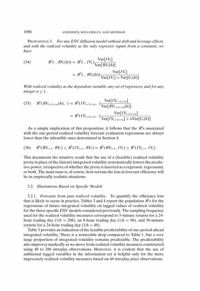
PROPOSITION 3. For any ESV diffusion model without drift and leverage effects,and with the realized volatility as the only regressor (apart from a constant), wehave

R2(·, RVt (h)) = R2(·, IVt )Var[IVt ]

Var[RVt (h)]

= R2(·, RVt (h))Var[IVt ]

Var[IVt ] + Var[Ut (h)]

(34)

With realized volatility as the dependent variable, any set of regressors, and for anyinteger n ≥ 1,

R2(RVt+1:t+n(h), ·) = R2(IVt+1:t+n, ·) Var[IVt+1:t+n]Var[RVt+1:t+n(h)]

= R2(IVt+1:t+n, ·) Var[IVt+1:t+n]Var[IVt+1:t+n] + nVar[Ut (h)]

(35)

As a simple implication of this proposition, it follows that the R2s associatedwith the one-period realized volatility forecast evaluation regressions are alwayslower than the infeasible ones determined in Section 4:

R2(RVt+1, RVt ) ≤ R2(IVt+1, RVt ) = R2(RVt+1, IVt ) ≤ R2(IVt+1, IVt )(36)

This documents the intuitive result that the use of a (feasible) realized volatilityproxy in place of the (latent) integrated volatility systematically lowers the predic-tive power, irrespective of whether the proxy is inserted as a regressor, regressand,or both. The main issue is, of course, how serious the loss in forecast efficiency willbe in empirically realistic situations.

5.2. Illustrations Based on Specific Models

5.2.1. Forecasts from past realized volatility. To quantify the efficiency lossthat is likely to occur in practice, Tables 3 and 4 report the population R2s for theregressions of future integrated volatility on lagged values of realized volatilityfor the three specific ESV models considered previously. The sampling frequencyused for the realized volatility measures correspond to 5-minute returns for a 24-hour trading day (1/h = 288), an 8-hour trading day (1/h = 96), and 30-minutereturns for a 24-hour trading day (1/h = 48).

Table 3 provides an indication of the feasible predictability of one-period-aheadintegrated volatility. There is a noticeable drop compared to Table 1, but a verylarge proportion of integrated volatility remains predictable. The predictabilityalso improves markedly as we move from realized volatility measures constructedusing 48 to 288 intraday observations. Moreover, it is evident that the use ofadditional lagged variables in the information set is helpful only for the moreimprecisely realized volatility measures based on 48 intraday price observations.


TABLE 3ONE-PERIOD-AHEAD FORECASTS OF INTEGRATED VOLATILITY BASED ON REALIZED VOLATILITY

M1 M2 M3Model1/h 48 96 288 48 96 288 48 96 288

R2(IVt+1, RVt(h)) 0.836 0.891 0.932 0.476 0.563 0.641 0.881 0.927 0.960R2(IVt+1, RVt(h), 1) 0.873 0.906 0.934 0.507 0.574 0.642 0.917 0.943 0.962R2(IVt+1, RVt(h), 4) 0.883 0.908 0.934 0.519 0.580 0.642 0.929 0.946 0.963R2(IVt+1, RVt(h), ARMA) 0.883 0.908 0.934 0.522 0.582 0.646 – – –

TABLE 4MULTI-PERIOD-AHEAD FORECASTS OF INTEGRATED VOLATILITY BASED ON REALIZED VOLATILITY

5 10 20Horizon1/h 48 96 288 48 96 288 48 96 288

Model M1R2(IVt+1:t+n, RVt(h)) 0.762 0.813 0.851 0.682 0.727 0.761 0.551 0.588 0.615R2(IVt+1:t+n, RVt(h), 1) 0.797 0.827 0.852 0.713 0.740 0.762 0.576 0.598 0.616R2(IVt+1:t+n, RVt(h), 4) 0.805 0.829 0.852 0.720 0.741 0.762 0.582 0.599 0.616R2(IVt+1:t+n, RVt(h), ARMA) 0.806 0.829 0.852 0.721 0.741 0.762 0.582 0.599 0.616

Model M2R2(IVt+1:t+n, RVt(h)) 0.307 0.364 0.414 0.226 0.268 0.305 0.148 0.175 0.199R2(IVt+1:t+n, RVt(h), 1) 0.339 0.381 0.419 0.255 0.285 0.312 0.169 0.188 0.205R2(IVt+1:t+n, RVt(h), 4) 0.360 0.395 0.429 0.277 0.302 0.325 0.186 0.202 0.216R2(IVt+1:t+n, RVt(h), ARMA) 0.368 0.400 0.434 0.286 0.309 0.330 0.194 0.208 0.221

Model M3R2(IVt+1:t+n, RVt(h)) 0.843 0.886 0.918 0.797 0.839 0.869 0.717 0.754 0.781R2(IVt+1:t+n, RVt(h), 1) 0.877 0.901 0.920 0.830 0.853 0.871 0.747 0.768 0.783R2(IVt+1:t+n, RVt(h), 4) 0.889 0.904 0.920 0.841 0.856 0.871 0.757 0.770 0.784

Table 4 considers the predictability of integrated volatility over longer horizons.For models M1 and M3, the conclusions mirror those for Table 3 discussed above.For model M2, it is increasingly obvious that more frequent sampling of the intra-day returns is beneficial. Likewise, for the scenarios with lower predictability—long horizons and relatively infrequent sampling of intraday returns—it is moreimportant to include additional explanatory variables in the formation of thevolatility forecasts.

Of course, the R2s reported above cannot be mimicked by actual data, sincethe left-hand-side variable of interest—integrated volatility—is not observable.Feasible regressions must rely on, e.g., ex post realized volatility measures as aproxy for the realization of future integrated volatility. Since the use of such a proxywill bias the observable predictability downward, it is important to recognize thesize of the potential bias. The relevant population R2 from such feasible regressionsmay be derived from (35). Moreover, combining the above result with (34) allowsfor the derivation of the fully feasible regression R2s based on realized volatility


TABLE 5ONE-PERIOD-AHEAD FORECASTS OF REALIZED VOLATILITY BASED ON REALIZED VOLATILITY

M1 M2 M3Model1/h 48 96 288 48 96 288 48 96 288

R2(RVt+1(h), RVt(h)) 0.731 0.832 0.911 0.328 0.460 0.597 0.795 0.879 0.943R2(RVt+1(h), RVt(h), 1) 0.765 0.846 0.912 0.350 0.469 0.597 0.827 0.894 0.945R2(RVt+1(h), RVt(h), 4) 0.773 0.848 0.912 0.358 0.474 0.600 0.838 0.897 0.945R2(RVt+1(h), RVt(h), ARMA) 0.773 0.848 0.912 0.360 0.475 0.601 – – –

TABLE 6MULTI-PERIOD-AHEAD FORECASTS OF REALIZED VOLATILITY BASED ON REALIZED VOLATILITY

5 10 20Horizon1/h 48 96 288 48 96 288 48 96 288

Model M1R2(RVt+1:t+n(h), RVt(h)) 0.740 0.801 0.847 0.671 0.722 0.759 0.546 0.585 0.614R2(RVt+1:t+n(h), RVt(h), 1) 0.774 0.815 0.848 0.702 0.734 0.760 0.571 0.595 0.615R2(RVt+1:t+n(h), RVt(h), 4) 0.782 0.816 0.848 0.709 0.735 0.760 0.577 0.597 0.615R2(RVt+1:t+n(h), RVt(h), ARMA) 0.782 0.816 0.848 0.709 0.735 0.760 0.577 0.597 0.615

Model M2R2(RVt+1:t+n(h), RVt(h)) 0.274 0.343 0.406 0.210 0.258 0.302 0.140 0.170 0.197R2(RVt+1:t+n(h), RVt(h), 1) 0.303 0.359 0.410 0.237 0.275 0.308 0.160 0.184 0.203R2(RVt+1:t+n(h), RVt(h), 4) 0.321 0.372 0.421 0.258 0.291 0.321 0.177 0.197 0.214R2(RVt+1:t+n(h), RVt(h), ARMA) 0.328 0.378 0.425 0.266 0.297 0.326 0.184 0.202 0.219

Model M3R2(RVt+1:t+n(h), RVt(h)) 0.824 0.876 0.914 0.788 0.834 0.867 0.713 0.752 0.781R2(RVt+1:t+n(h), RVt(h), 1) 0.858 0.891 0.917 0.821 0.848 0.869 0.742 0.765 0.783R2(RVt+1:t+n(h), RVt(h), 4) 0.869 0.895 0.917 0.832 0.851 0.869 0.752 0.768 0.783

proxies for integrated volatility, both as regressor and regressand. Tables 5 and 6report on the amount of predictability associated with such feasible regressions.

Compared to Table 3, Table 5 reveals a significant loss of predictive power, evenfor models M1 and M3. Of course, this is purely artificial as it is induced solelyby the measurement error in the integrated volatility proxy. Nonetheless, the R2sstill reveal a large amount of verifiable predictability in the integrated (realized)volatility process. As before, we also find that the impact of measurement errorsis mitigated when more frequent sampling is undertaken.16

16 Barndorff-Nielsen and Shephard (2002a) provide complementary one-period-ahead forecast ofintegrated volatility based on realized volatilities. Their (model-based) approach uses the state-spacerepresentation of the integrated volatility (combined with the Kalman filter) when the spot variancedepends on autoregressive and independent factors, as in models M1 and M2. Indeed, for these twomodels, their one-period-ahead forecasts correspond exactly to our forecasts based on the ARMArepresentation of the realized volatility provided in Table 5.


Table 6 extends the results in Table 5 to longer forecast horizons. The generalconclusions are reinforced, but one interesting difference from Tables 3 and 4 be-comes apparent. It is now possible for the five-period-ahead forecasts to display ahigher degree of predictability than the one-period-ahead forecasts, as evidencedby the results for models M1 and M3 with a sampling frequency of 1/h = 48. Thisoccurs because the realization of integrated volatility is approximated more accu-rately over five periods as opposed to just one period, relative to the true variabilityin the latent integrated volatility. Thus, the decline in fundamental predictabilityassociated with a longer horizon is more than offset by the relatively smaller mea-surement error in the dependent variable.17 This provides a vivid illustration of theimportance of recognizing the downward bias in the true predictability inducedby the need to rely on an observable proxy for the ex post integrated volatilityrealizations. At the same time, it is clear that the downward bias is almost nonex-istent for the longer 20-period horizon, where the R2 figures in Table 6 are veryclose to those in Table 4 across all models and sampling frequencies.

5.2.2. Forecasts from past daily squared returns. To highlight the improved“signal-to-noise ratio” achieved by employing the realized volatility measuresbased on high-frequency intraday data rather than the traditional approach thatonly relies on daily data, we finally consider the results related to the forecasts ofintegrated and realized volatility based on past daily squared returns, i.e., h = 1.

The first panel of Table 7 demonstrates that it is critical to employ long lagsof daily squared returns in order to predict future (integrated) volatility withany accuracy. Consistent with the general weak GARCH principle of Drost andWerker (1996) and Meddahi (2003), it is evident how effective a simple (recursive)GARCH structure is in parsimoniously capturing the information in the laggedsquared daily returns. However, even in the best of circumstances, a comparisonof the upper panel in Table 7 with Tables 3 and 4 reveals that the forecast ef-ficiency is severely curtailed by restricting the information set to the history ofdaily squared returns rather than the past realized volatilities constructed fromthe high-frequency data.

The lower panels of Table 7 provide corresponding evidence for feasible volatil-ity forecast regressions where the integrated volatility regressor is replaced by(feasible) realized volatility approximations computed from sampling frequen-cies ranging from 288 intraday observations (5-minute returns covering 24 hours)to daily data. The use of daily squared returns as a one-step-ahead volatility proxyis representative of much of the empirically oriented volatility literature over thelast decade. The use of cumulative squared daily returns as a volatility measureover longer weekly, monthly, and quarterly horizons has been emphasized byFrench et al. (1987) and Schwert (1989, 1990), among others.

For all scenarios in the lower panels of Table 7, we inevitably find an even lowerdegree of predictability than implied by the corresponding integrated volatility

17 Formally, in (35) the last equation will have the fundamental predictability, R2(IVt+1:t+n, ·),decline with n, but the ratio Var[IVt+1:t+n]/Var[RVt+1:t+n(h)] will increase with n, and for lowervalues of 1/h this may actually raise the observed R2.


TABLE 7FORECASTS OF INTEGRATED AND REALIZED VOLATILITIES FROM PAST DAILY SQUARED RETURNS

M1 M2 M3Model

Horizon 1 5 10 20 1 5 10 20 1 5 10 20

IV lag0 0.122 0.111 0.100 0.081 0.031 0.020 0.015 0.010 0.157 0.150 0.142 0.1281 0.210 0.191 0.171 0.138 0.048 0.033 0.025 0.017 0.266 0.255 0.241 0.2174 0.360 0.329 0.294 0.238 0.072 0.054 0.043 0.029 0.452 0.432 0.409 0.369

19 0.493 0.450 0.402 0.325 0.092 0.074 0.061 0.043 0.639 0.611 0.580 0.52339 0.498 0.454 0.406 0.328 0.093 0.075 0.062 0.044 0.653 0.625 0.593 0.535

GARCH 0.498 0.454 0.406 0.328 0.093 0.075 0.062 0.044 – – – –

1/h lag

288 0 0.119 0.110 0.099 0.080 0.029 0.019 0.015 0.009 0.154 0.149 0.142 0.1281 0.205 0.190 0.171 0.138 0.044 0.032 0.024 0.016 0.261 0.254 0.241 0.217

4 0.352 0.327 0.293 0.238 0.066 0.052 0.042 0.029 0.444 0.430 0.408 0.36919 0.482 0.448 0.401 0.325 0.085 0.072 0.060 0.043 0.628 0.609 0.579 0.52239 0.486 0.452 0.405 0.328 0.086 0.074 0.061 0.043 0.641 0.623 0.592 0.534

GARCH 0.486 0.452 0.405 0.328 0.086 0.074 0.061 0.043 – – – –

96 0 0.114 0.109 0.099 0.080 0.025 0.019 0.014 0.009 0.149 0.148 0.141 0.1281 0.196 0.188 0.170 0.137 0.039 0.031 0.024 0.016 0.252 0.252 0.240 0.2164 0.336 0.324 0.292 0.237 0.058 0.050 0.040 0.028 0.429 0.427 0.407 0.368

19 0.460 0.443 0.399 0.324 0.075 0.069 0.058 0.042 0.606 0.604 0.577 0.52139 0.465 0.447 0.403 0.327 0.076 0.070 0.059 0.043 0.619 0.618 0.590 0.533

GARCH 0.465 0.447 0.403 0.327 0.076 0.070 0.059 0.043 – – – –

48 0 0.107 0.108 0.098 0.080 0.021 0.018 0.014 0.009 0.142 0.147 0.140 0.1271 0.184 0.185 0.168 0.137 0.033 0.029 0.023 0.016 0.240 0.249 0.238 0.2164 0.315 0.319 0.289 0.236 0.049 0.048 0.039 0.029 0.408 0.423 0.404 0.367

19 0.432 0.437 0.396 0.322 0.063 0.066 0.056 0.042 0.576 0.598 0.573 0.52039 0.436 0.441 0.400 0.325 0.064 0.067 0.057 0.043 0.589 0.611 0.586 0.532

GARCH 0.436 0.441 0.400 0.325 0.064 0.067 0.057 0.043 – – – –

1 0 0.016 0.046 0.057 0.057 0.001 0.003 0.003 0.003 0.026 0.073 0.092 0.0991 0.027 0.079 0.098 0.098 0.002 0.005 0.005 0.005 0.043 0.123 0.156 0.1684 0.046 0.136 0.168 0.167 0.003 0.008 0.009 0.008 0.073 0.209 0.264 0.286

19 0.063 0.185 0.229 0.229 0.004 0.011 0.013 0.012 0.103 0.295 0.374 0.40539 0.064 0.187 0.232 0.231 0.004 0.012 0.014 0.013 0.105 0.302 0.383 0.415

GARCH 0.064 0.187 0.232 0.231 0.004 0.012 0.014 0.013 – – – –

regressions. This is an immediate consequence of Equations (34) and (35).Nonetheless, for h = 1/288 or 1/96 we have sufficiently good approximationsto integrated volatility that the qualitative results are very similar to those in theupper panel, and even for h = 1/48 the loss in observed forecast power is limited.As such, this reinforces the conclusion from above: The (observable) forecast ef-ficiency is severely curtailed if one uses only the past daily returns in forecastingthe future volatility.

The bottom panel of Table 7 further documents the extraordinarily poor co-herence between future daily squared returns and the (near) optimal forecastsconstructed from past daily squared returns. Again, for the case where the real-ized volatility proxy works very poorly, the R2s actually increase with the forecast


horizon—now often dramatically so—illustrating the significance of the measure-ment error in a single day’s squared return relative to the corresponding volatility.It is evident across all forecast horizons that the true predictability of integratedvolatility is wildly underestimated by the R2 from these feasible regressions basedon volatility measures constructed from daily data. This is consistent with thefindings from the large literature trying to evaluate the performance of alterna-tive volatility forecasts by studying the R2 from the associated Mincer–Zarnowitzregressions using daily squared returns as the ex post volatility measure. Suchstudies invariably find the relative performance to be unstable and to differ acrossboth asset classes and time periods. This is what one should expect if the depen-dent variable of interest—realized ex post (integrated) volatility—is measuredwith a large degree of imprecision. Even for long daily samples, the findingsare largely random. Only by moving toward more meaningful ex post realizedvolatility measures for integrated volatility does it become possible to assess theforecast performance with any degree of reliability. This is, of course, exactly thepoint elaborated in Andersen and Bollerslev (1998). In fact, the current exposi-tion for predictability of volatility based on daily squared returns may be seen asan analytic extension to a much broader range of models of the simulation-basedinvestigation of the continuous-time GARCH model in Andersen and Bollerslev(1998) and Andersen et al. (1999).18

6. CONCLUSION

This article develops a direct analytic approach to the construction and assess-ment of volatility forecasts for continuous-time diffusion models within the broadESV class of models. This class incorporates the most popular volatility diffu-sion models in current use, and may be calibrated to account well for the majorempirical features of asset return volatility. The results provide theoretical upperbounds for the degree of predictability based on optimal (infeasible) forecastsalong with direct measures of the loss in forecast efficiency associated with lessprecise, but more practical (feasible) reduced-form realized volatility-based pro-cedures. As such, our results provide theoretical foundation and inspiration for thefurther development of new and improved easy-to-implement empirical volatil-ity forecasting procedures guided by proper (optimal) benchmark comparisons.The insights obtained from empirical comparisons of options implied volatilitiesmay, likewise, be improved by properly accounting for the volatility error. Thetechniques developed here could also be used in more effectively calibrating thetype of continuous-time models routinely employed in modern asset-pricing the-ories. We leave further theoretical and empirical work along these lines for futureresearch.

18 Specifically, the entry in Table 7, Panel 1, M1, row GARCH, corresponds directly to the entrym= ∞ (infinitely frequent sampling) for DM-dollar in Table 4 of Andersen and Bollerslev (1998). Theminor discrepancy between the numbers is due to the presence of small simulation errors in Andersenand Bollerslev (1998).


APPENDIX

We start out with the proofs of two useful lemmas.

LEMMA 1. For any ESV model,

E[∫ h

0Pi ( fu) du

∫ h

0Pj ( fu) du

]= δi j

2λ2

i

[exp(−λi h) + λi h − 1](A.1)

where δi j = 1 if i = j and δi j = 0 if i = j . Moreover, for n ≥ 1,

E

[∫ h

0Pi ( fu) du

∫ (n+1)h

nhPj ( fu) du

]

= δi j exp(−λ j (n − 1)h)[1 − exp(−λi h)]2

λ2i

(A.2)

PROOF OF LEMMA 1. Fubini’s Theorem implies that

∫ h

0Pi ( fu) du

∫ h

0Pj ( fu) du =

∫ h

0

∫ h

0Pi ( fu)Pj ( fs) du ds,

for a given path of the process f u, u ∈ [0, h]. In addition, we have

∫ h

0

∫ h

0Pi ( fu)Pj ( fs) du ds =

∫ h

0Pi ( fu)

(∫ u

0Pj ( fs) ds

)du

+∫ h

0Pj ( fu)

(∫ u

0Pi ( fs) ds

)du

Hence,

E[∫ h

0Pi ( fu) du

∫ h

0Pj ( fu) du

]

=∫ h

0

(∫ u

0E[Pi ( fu)Pj ( fs)] ds

)du +

∫ h

0

(∫ u

0E[Pj ( fu)Pi ( fs)] ds

)du

=∫ h

0

(∫ u

0exp(−λi (u − s))E[Pi ( fs)Pj ( fs)] ds

)du

+∫ h

0

(∫ u

0exp(−λ j (u − s))E[Pj ( fs)Pi ( fs)] ds

)du,

= 2δi j

∫ h

0

(∫ u

0exp(−λi (u − s)) ds

)du = δi j

2λ2

i

[exp(−λi h) + λi h − 1]


where the second and third equalities follow from (10) and (9), respectively. Equa-tion (A.2) follows from

E

[∫ h

0Pi ( fu) du

∫ (n+1)h

nhPj ( fu) du

]

= E

[∫ h

0Pi ( fu) du

∫ (n+1)h

nhE[Pj ( fu) | fτ , τ ≤ h] du

]

= E

[∫ h

0Pi ( fu) du

∫ (n+1)h

nhexp(−λ j (u − h))Pj ( fh) du

]

= exp(−λ j (n − 1)h)1 − exp(−λi h)

λi

∫ h

0E[Pi ( fu)Pj ( fh)] du

= δi j exp(−λ j (n − 1)h)[1 − exp(−λi h)]2

λ2i

. �

LEMMA 2. Let the ARMA(2,2) model for yt be denoted by

yt = µ + φ1 yt−1 + φ2 yt−2 + ηt + θ1ηt−1 + θ2ηt−2

where ηt is a weak white noise. Then,

R2(yt+1:t+n, ARMA) = 1 − Var[yt+1:t+n − BP[yt+1:t+n | Ht (y)]]Var[yt+1:t+n]

(A.3)

with

Var[yt+1:t+n − BP[yt+1:t+n | Ht (y)]] =n−1∑i=0

(i∑

s=0

ψs

)2

Var[ηt ](A.4)

where ψ i = A�1 �i A2, with A1 = (1, 0, 0, 0)�, A2 = (1, 0, 1, 0)�, � is a 4 × 4 matrix

with �[1, 1] = φ1, �[1, 2] = φ2, �[1, 3] = θ1, �[1, 4] = θ2, �[2, 1] = 1, �[4, 3] = 1,and 0 otherwise, Ht(z) denotes the Hilbert-space generated by {1, zτ , τ ≤ t}, whereasfor a second-order stationary variable w, BP[w | Ht(z)] denotes the best linear pre-dictor of w given Ht(z); i.e., w = BP[w | Ht(z)] + ε, with Cov(ε, x) = 0, ∀x ∈Ht(z).

PROOF OF LEMMA 2. Following Baillie and Bollerslev (1992),

yt+n − BP[yt+n | Ht (y)] =n−1∑i=0

ψiηt+n−i


for any n > 0. Therefore, one obtains the following two equalities:

yt+1:t+n − BP[yt+1:t+n | Ht (y)] =n−1∑i=0

(i∑

s=0

ψs

)ηt+n−i

Var[yt+1:t+n − BP[yt+1:t+n | Ht (y)]] =n−1∑i=0

(i∑

s=0

ψs

)2

Var[ηt ]

i.e., (A.4). Note that although the results of Baillie and Bollerslev (1992) arederived under the assumption that ηt is a martingale difference sequence andrefers to E[yt+n | yτ , τ ≤ t] rather than BP[yt+n | Ht(y)], the final result remainsvalid when ηt is a weak white noise process (as for the integrated and realizedvolatilities); see also Meddahi and Renault (2004) and Meddahi (2003) for furtherdiscussion along these lines. Finally, observe that when φ2 = θ2 = 0, i.e., yt is anARMA(1,1), (A.3) becomes

R2(yt+1:t+n, ARMA) =(1 − φn

1

)2

(1 − φ1)2

Var[yt ]Var[yt+1:t+n]

R2(yt+1, ARMA)(A.5)

PROOF OF PROPOSITION 1. Given that the unconditional mean of any eigen-function Pi(·), with i ≥ 1, is zero, one gets (12). Let s be a positive real; then wehave

E[σ 2

t+s

∣∣ Sτ , fτ , τ ≤ t] =

p∑i=0

ai E[Pi ( ft+s) | ft ] = a0 +p∑

i=1

ai exp(−λi s)Pi ( ft )(A.6)

which corresponds to (13) for s = n. By using (A.6), one can show easily

E[IVt+n | Sτ , fτ , τ ≤ t] = a0 +p∑

i=1

ai exp(−λi (n − 1))(1 − exp(−λi ))

λiPi ( ft )(A.7)

Therefore,

E[IVt+1:t+n | Sτ , fτ , τ ≤ t]

= na0 +n∑

s=1

p∑i=1

ai exp(−λi (s − 1))[1 − exp(−λi )]

λiPi ( ft )

= na0 +p∑

i=1

ai

(n∑

s=1

exp(−λi (s − 1))

)[1 − exp(−λi )]

λiPi ( ft )

= na0 +p∑

i=1

ai[1 − exp(−λi n)]

λiPi ( ft )


i.e., (14). The first result in (15) follows from the orthonormality of the eigenfunc-tion, indicated in (9). In addition, for any real s ≥ 0

Var

[∫ t−1+s

t−1σ 2

u du

]= E

(p∑

i=1

ai

∫ t−1+s

t−1Pi ( fu) du

)2

=∑

1≤i, j≤p

ai ai E

[∫ t−1+s

t−1Pi ( fu) du

∫ t−1+s

t−1Pj ( fu) du

]

=∑

1≤i, j≤p

ai aiδi j2λ2

i

[exp(−λi s) + λi s − 1]

where the last equality follows from (A.1). Thus,

Var

[∫ t−1+s

t−1σ 2

u du

]= 2

p∑i=1

a2i

λ2i

[exp(−λi s) + λi s − 1](A.8)

which corresponds to the second result in (15) for s = n. By using the orthonor-mality of the eigenfunctions, Equations (A.7), and the equality, Cov(IVt+n, σ 2

t ) =Cov(E[IVt+n | Sτ , f τ , τ ≤ t], σ 2

t ), it follows that

Cov(IVt+n, σ

2t

) =p∑

i=1

a2i exp(−λi (n − 1))


(A.9)

Hence,

Cov(IVt+1:t+n, σ

2t−l

) =n∑

s=1

p∑i=1

a2i exp(−λi (s + l − 1))


=p∑

i=1

a2i exp(−λi l)

(n∑

s=1

exp(−λi (s − 1))

)[1 − exp(−λi )]

λi

=p∑

i=1

a2i


exp(−λi l)

i.e., (16). Equation (18) is obtained by a similar argument. By using (A.2), onegets


Cov(IVt , IVt+n) = Cov(IV1, IV1+n)

= E

[(p∑

i=0

ai

∫ 1

0Pi ( fu) du

) (p∑

i=1

ai

∫ n+1

nPi ( fu) du

)]

=∑

1≤i, j≤p

ai a j E

[∫ 1

0Pi ( fu) du

∫ n+1

1Pj ( fu) du

]

=∑

1≤i, j≤p

ai a jδi j exp(−λi (n − 1))[1 − exp(−λi )]2

λ2i

=p∑

i=1

a2i exp(−λi (n − 1))

[1 − exp(−λi )]2

λ2i

(A.10)

Utilizing (A.10) in a similar set of arguments, it is possible to show (17). �

PROOF OF PROPOSITION 2. By straightforward calculations, it is easy to show

∀λ > 0,[1 − exp(−λ)]2

exp(−λ)≥ λ2 ≥ 2[exp(−λ) + λ − 1](A.11)

2[exp(−λ) + λ − 1][1 − exp(−λ)]

≥ λ ≥ [1 − exp(−λ)](A.12)

Thus, by using the first inequality in (A.11), it follows that for any n ≥ 1,

exp(−λn) ≤ exp(−λ(n − 1))[1 − exp(−λ)]2λ−2

so that Cov(σ 2t+n, σ 2

t ) ≤ Cov(IVt+n, IVt). Also, by using the second inequality in(A.12), one gets [1 − exp(−λ)]2λ−2 ≤ [1 − exp(−λ)]λ−1 ≤ 1. Therefore,

∀n ≥ 1, exp(−λ(n − 1))[1 − exp(−λ)]2λ−2

≤ exp(−λ(n − 1))[1 − exp(−λ)]λ−1 ≤ 1,

and, hence, Cov(IVt+n, IVt) ≤ Cov(IVt+n, σ 2t ). The first inequality in (A.12)

implies

∀n ≥ 1, exp(−λ(n − 1))[1 − exp(−λ)]λ−1

≤ [1 − exp(−λ)]λ−1 ≤ 2[exp(−λ) + λ − 1]λ−2,

and, hence, Cov(IVt+n, σ 2t ) ≤ Var[IVt]. Finally, by the second inequality in (A.11),

Var[IVt] ≤ Var[σ 2t ], which completes the proof of Proposition 2. �


PROOF OF (20). R2(IVt+1, Best) equals Var[E[IVt+1 | Sτ , f τ , τ ≤ t]]/Var[IVt+1]. By using (A.7) for n = 1 along with the orthonormal-ity of the eigenfunctions, i.e., (9), we get Var[E[IVt+1 | Sτ , fτ , τ ≤ t]] =∑p

i=1 a2i [1 − exp(−λi )]2λ−2

i , which combines to show (20). �

PROOF OF (21) AND (22). By definition, we have

R2(IVt+1, σ2t

) = Cov(IVt+1, σ

2t

)2/Var[IVt+1]Var[σ 2

t

]Thus, by using (16) for n = 1, we get (21). A similar argument leads to (22). �

Formulas for R2s Based on Multiple Explanatory Variables.

R2(IVt+1, IVt , l) = C(IVt+1, IVt , l)�(M(IVt , l))−1C(IVt+1, IVt , l)/Var[IVt ]

R2(IVt+1:t+n, σ2t , l

) = C(IVt+1:t+n, σ

2t , l

)�M

(σ 2

t , l)−1

C(IVt+1:t+n, σ

2t , l

)Var[IVt+1:t+n]

R2(IVt+1:t+n, IVt , l) = C(IVt+1:t+n, IVt , l)�M(IVt , l)−1C(IVt+1:t+n, IVt , l)Var[IVt+1:t+n]

Formulas for R2s Based on Multi-Step-Ahead Integrated Volatility. These fol-low by a simple application of Lemma A.2. The ARMA representation of inte-grated volatility is given in Meddahi (2003). �

PROOF OF PROPOSITION 3. Let y be a second-order stationary variable such thatCov(y, Ut(h)) = 0. Then

R2(y, RVt (h)) = Cov(y, RVt (h))2

Var[y]Var[RVt (h)]= Cov(y, IVt + Ut (h))2

Var[y]Var[RVt (h)]

= Cov(y, IVt )2

Var[y]Var[IVt ]Var[IVt ]

Var[RVt (h)]

i.e., (34). Furthermore, for any n ≥ 1 and h > 0, BP[RVt+1:t+n(h) | Ht(RV(h))]equals BP[IVt+1:t+n | Ht(RV(h))] given that RVt+i (h) = IVt+i + Ut+i (h), whereasUt+i (h), i ≥ 1, is uncorrelated with any variable in Ht(RV(h)). Note that the sameresults hold if one considers the best predictor (of RVt+1:t+n(h) or IVt+1:t+n) givenlags of RVt(h) (and a constant). Hence, BP[RVt+1:t+n(h) | .] = BP[IVt+1:t+n | .],and


R2(RVt+1:t+n(h), .) = Var[BP[RVt+1:t+n(h) | .]]Var[RVt+1:t+n(h)]

= Var[BP[IVt+1:t+n | .]]Var[RVt+1:t+n(h)]

= Var[BP[IVt+1:t+n | .]]Var[IVt+1:t+n]

Var[IVt+1:t+n]Var[RVt+1:t+n(h)]

= R2(IVt+1:t+n, .)Var[IVt+1:t+n]

Var[IVt+1:t+n] + nVar[Ut (h)],

i.e., (35). �

REFERENCES

AıT-SAHALIA, Y., L. P. HANSEN, AND J. SCHEINKMAN, “Operator Methods for Continuous-Time Markov Models,” in Y. Ait-Sahalia and L. P. Hansen, eds., Handbook of FinancialEconometrics (Amsterdam: North Holland Press, 2005), forthcoming.

ALIZADEH, S., M. BRANDT, AND F. DIEBOLD, “Range-Based Estimation of Stochastic Volatil-ity Models,” Journal of Finance 57 (2002), 1047–91.

ANDERSEN, T. G., AND T. BOLLERSLEV, “Answering the Skeptics: Yes, Standard VolatilityModels Do Provide Accurate Forecasts,” International Economic Review 39 (1998),885–905.

——, L. BENZONI, AND J. LUND, “An Empirical Investigation of Continuous-Time EquityReturn Models,” Journal of Finance 57 (2002), 1239–84.

——, T. BOLLERSLEV, AND F. X. DIEBOLD, “Parametric and Nonparametric Measurementsof Volatility,” in Y. Aıt-Sahalia and L. P. Hansen, eds., Handbook of Financial Econo-metrics (Amsterdam: North Holland Press, 2005), forthcoming.

——, ——, AND S. LANGE, “Forecasting Financial Market Volatility: Sample Frequencyvis-a-vis Forecast Horizon,” Journal of Empirical Finance 6 (1999), 457–77.

——, ——, F. X. DIEBOLD, AND P. LABYS, “Modeling and Forecasting Realized Volatility,”Econometrica 71 (2003), 579–625.

——, ——, ——, AND ——, “The Distribution of Exchange Rate Volatility,” Journal of theAmerican Statistical Association 96 (2001), 42–55.

ANDREOU, E., AND E. GHYSELS, “Rolling-Sampling Volatility Estimators: Some New Theo-retical, Simulation and Empirical Results,” Journal of Business and Economic Statistics20 (2002), 363–76.

BAILLIE, R. T., AND T. BOLLERSLEV, “Prediction in Dynamic Models with Time-DependentConditional Variances,” Journal of Econometrics 52 (1992), 91–113.

BARNDORFF-NIELSEN, O. E., AND N. SHEPHARD, “Non-Gaussian OU Based Models and Someof Their Uses in Financial Economics” (with discussion), Journal of the Royal StatisticalSociety B 63 (2001), 167–241.

——, AND ——, “Econometric Analysis of Realised Volatility and Its Use in EstimatingStochastic Volatility Models,” Journal of the Royal Statistical Society B 64 (2002a),253–80.

——, AND ——, “Estimating Quadratic Variation Using Realised Variance,” Journal ofApplied Econometrics 5 (2002b), 457–77.

——, AND ——, Financial Volatility and Levy Based Models, Nuffield College, OxfordUniversity, 2004, forthcoming.

BILLINGSLEY, P., Probability and Measure (New York: John Wiley & Sons, 1986).BOLLERSLEV, T., AND H. ZHOU, “Estimating Stochastic Volatility Diffusion Using Condi-

tional Moments of Integrated Volatility,” Journal of Econometrics 109 (2002), 33–65.CAMPBELL, B., N. MEDDAHI, AND E. SENTANA, “Understanding Long-Horizon Predictability

of Asset Returns,” Universite of Montreal Working Paper, 2004.


CHEN, X., L. P. HANSEN, AND J. SCHEINKMAN, “Principal Components and the Long Run,”University of Chicago Working Paper, 2000.

CHONG, Y. Y., AND D. HENDRY, “Econometric Evaluation of Linear Macro-Economic Mod-els,” Review of Economic Studies 53 (1986), 671–90.

CHRISTOFFERSEN, P. F., AND F. X. DIEBOLD, “How Relevant is Volatility Forecasting forFinancial Risk Management,” Review of Economics and Statistics 81 (2000), 12–22.

COMTE, F., AND E. RENAULT, “Long Memory in Continuous Time Stochastic Volatility Mod-els,” Mathematical Finance 8 (1998), 291–323.

DROST, F. C., AND T. E. NIJMAN, “Temporal Aggregation of GARCH Processes,” Econo-metrica 61 (1993), 909–27.

——, AND B. J. M. WERKER, “Closing the GARCH Gap: Continuous Time GARCH Mod-eling,” Journal of Econometrics 74 (1996), 31–58.

ENGLE, R. F., “The Econometrics of Ultra-High Frequency Data,” Econometrica 68 (2000),1–22.

——, AND G. G. J. LEE, “A Permanent and Transitory Component Model for Stock ReturnVolatility,” in R. F. Engle and H. White, eds., Cointegration, Causality and Forecasting:a Festschrift in Honour of Clive W.J. Granger (New York: Oxford University Press,1999), 475–97.

FRENCH, K. R., G. W. SCHWERT, AND R. F. STAMBAUGH, “Expected Stock Returns and Volatil-ity,” Journal of Financial Economics 19 (1987), 3–29.

GALLANT, R., AND G. TAUCHEN, “Simulated Score Methods and Indirect Inference forContinuous-Time Models,” in Y. Aıt-Sahalia and L. P. Hansen, eds., Handbook ofFinancial Econometrics (Amsterdam: North Holland Press, 2005), forthcoming.

——, C. HSU, AND G. TAUCHEN, “Using Daily Range Data to Calibrate Volatility Diffusionsand Extract the Forward Integrated Variance,” Review of Economics and Statistics 81(1999), 617–31.

GARCIA, R., M. A. LEWIS, AND E. RENAULT, “Estimation of Objective and Risk-NeutralDistributions Based on Moments of Integrated Volatility,” Working Paper, Universityof Montreal, 2001.

HANSEN, L. P., AND J. SCHEINKMAN, “Back to the Future: Generating Moment Implicationsfor Continuous Time Markov Processes,” Econometrica 63 (1995), 767–804.

HARVEY, A. C., E. RUIZ, AND N. SHEPHARD, “Multivariate Stochastic Variance Models,”Review of Economic Studies 61 (1994), 247–64.

HESTON, S. L., “A Closed Form Solution for Options with Stochastic Volatility with Appli-cations to Bond and Currency Options,” Review of Financial Studies 6 (1993), 327–44.

HOFFMAN-JøRGENSEN, J., Probability with a View Toward Statistics, Volume 1 (New York:Chapman & Hall, 1994).

HULL, J., AND A. WHITE, “The Pricing of Options on Assets with Stochastic Volatilities,”Journal of Finance 42 (1987), 281–300.

JOHANNES, M., AND N. POLSON, “Numerical Bayesian Methods for Estimating Continuous-Time Models,” in Y. Aıt-Sahalia and L. P. Hansen, eds., Handbook of Financial Econo-metrics (Amsterdam: North Holland Press, 2005), forthcoming.

MEDDAHI, N., “An Eigenfunction Approach for Volatility Modeling,” CIRANO WorkingPaper 2001s-70, 2001.

——, “A Theoretical Comparison Between Integrated and Realized Volatility,” Journal ofApplied Econometrics 17 (2002), 479–508.

——, “ARMA Representation of Integrated and Realized Variances,” The EconometricsJournal 6 (2003), 334–55.

——, AND E. RENAULT, “Temporal Aggregation of Volatility Models,” Journal of Econo-metrics 119 (2004), 355–79.

MINCER, J., AND V. ZARNOWITZ, “The Evaluation of Economic Forecasts,” in J. Mincer, ed.,Economic Forecasts and Expectation (New York: National Bureau of Research, 1969),3–46.

NELSON, D. B., “ARCH Models as Diffusion Approximations,” Journal of Econometrics 45(1990) 7–39.


SCHWERT, G. W., “Stock Volatility and the Crash of ’87,” Review of Financial Studies 3(1990), 77–102.

——, “Why Does Stock Market Volatility Change Over Time?” Journal of Finance 44(1989), 1115–54.

SZEGO, G., Orthogonal Polynomials, 4th edition (Providence, RI: American MathematicalSociety, 1975).

WIGGINS, J. B., “Options Values under Stochastic Volatility: Theory and Empirical Esti-mates,” Journal of Financial Economics 19 (1987), 351–72.

WONG, E., “The Construction of a Class of Stationary Markoff Processes,” in R. Belleman,ed., Sixteenth Symposium in Applied Mathematics, Stochastic Processes in Mathemati-cal Physics and Engineering (Providence, RI: American Mathematical Society, 1964),264–76.

Documents

ANALYTICAL EVALUATION OF VOLATILITY FORECASTS