Embed Size (px)
Citation preview

The Distortionary Effects of Market
Microstructure Noise on Volatility
Forecasts
Derek Cong Song
April 19, 2010
Professor George Tauchen, Faculty Advisor
Professor Tim Bollerslev, Faculty Advisor
Honors thesis submitted in partial fulfillment of the requirements for Graduationwith Distinction in Economics in Trinity College of Duke University.
The Duke Community Standard was upheld in the completion of this paper.
I will be working towards a PhD in Economics at Northwestern Universitybeginning Fall 2010. I can be reached at [email protected].
Duke University
Durham, North Carolina
2010

Acknowledgments
I am extremely grateful to Professor George Tauchen for his invaluable mentorship
through the entire thesis process. I would also like to thank Professor Tim Bollerslev
for his insightful comments and his help in guiding me to my research topic. Addi-
tionally, I would like to thank all of my classmates in the Honors Finance Seminars,
Econ 201FS and Econ 202FS, for their ideas and feedback.
2
Abstract
In volatility estimation, the use of high-frequency price data allows us to obtain
better estimates of the market’s true volatility level. However, when the data is
sampled in very small increments, market microstructure noises can distort those
estimates. This paper seeks to empirically examine the impact of microstructure noise
on volatility forecasting by testing the robustness of different models and estimation
to the sampling interval using a HAR framework (Corsi, 2003). In particular, we
looked at sparse and sub-sampled estimators, implied volatility, and OLS and robust
regressions. The models were evaluated based on their out-of-sample performance on
one-month-ahead volatility forecasts. Our results show that in HAR models may be
quite sensitive to the presence of noise. However, the inclusion of implied volatility
coupled with a robust estimation procedure improved the models’ robustness. These
findings suggest that while noise can be extremely disruptive, forecasting models can
be constructed in certain ways to make them significantly more robust to noise.
3

1 Introduction
Volatility and risk in financial markets is an extremely important field of study in
financial econometrics. Research on estimating and forecasting volatility is especially
crucial in applications such as risk management and asset pricing (the fair price of
options, for instance, are in part determined by the expected future level of volatility).
In the past, the only available asset prices were the daily opens and closes, making any
estimates of volatility fairly unreliable due to the lack of information about intraday
price movements. In recent years, the availability of high-frequency data (‘frequency’
here refers to how often prices are recorded, e.g. every second, minute, or hour)
has given rise to new models of volatility that have yielded significant improvements
in the accuracy of volatility measurements and forecasting (Andersen and Bollerslev
(1998)).
Generally, a stock is assumed to have a ‘true’ price whose evolution over time can
be modeled as a continuous stochastic process. The theoretical advantage of using
high-frequency data comes from being able to better approximate the (continuous)
sample path of this price process, producing more accurate estimates of the process’s
variance. However, the assumption that higher resolutions necessarily equates to
better approximations is only valid up to a certain point. At extremely high frequen-
cies (for example, prices sampled every minute), various market frictions inherent
in the trading process begin to manifest as first order effects, potentially distorting
the values obtained using this approach. Collectively, these frictions are referred to
as market microstructure noise. As discussed in Aıt-Sahalia and Yu (2009), market
microstructure noise can arise from factors such as bid-ask bounce, discreteness of
prices, variations in trade sizes, differences in the informational usefulness of price
changes, market responses to strategic moves (block trades, for example), etc. Mar-
4

ket microstructure is an important consideration for high-frequency data because as
we probe the data at increasingly smaller scales, the signal-to-noise ratio can fall dra-
matically, to the point where the noise may overwhelm everything else. As a result,
the higher the frequencies used to obtain the estimates, the more unreliable they tend
to become.
As we might expect, for high-frequency data, it is a non-trivial task to sample
prices in an appropriate way. The sampling interval must be chosen so as to balance
data utilization with robustness to noise. The basic sampling method, called sparse
sampling, simply involves producing a volatility estimate from some subset of the
prices. There are several other advanced sampling techniques which have been found
to improve on sparse estimation, including the one that will be discussed in this paper,
sub-sampling. The sub-sampled estimator can be thought of as an average of the
sparse estimators over different grids, the idea being to waste less of the data. For an
overview of other methods, consult Andersen, Bollerslev, and Meddahi (2006). There
is also a proposed optimal frequency that seeks to identify the sampling interval that
minimizes the volatility estimator relative to some measure of fit (e.g., minimizing the
mean squared errors of the volatility estimates, in the context of forecasting errors).
However, in practice, sampling intervals are often chosen heuristically, without first
looking at the viability of the other possible sampling intervals. While this approach
is certainly more convenient, it is not clear whether the performance of the different
sampling schemes depends at all on what sampling interval was chosen. It may be
that other choices of sampling intervals could yield better estimates and predictions.
This paper adds to the existing literature on volatility estimation by being the first
to systematically examine the empirical impact of the sampling interval and market
microstructure noise on volatility forecasts. In particular, the objective is to study
5

how the forecasting accuracy under different models and sampling techniques respond
to different choices of sampling interval. Ultimately, we hope to identify some of the
conditions under which sampling intervals, and by extension market microstructure
noise, can influence regressions.
We begin by estimating the daily volatilities of a constructed portfolio of 40 stocks
using two different sampling techniques at intervals of 1 minute up to 30 minutes.
The data sample is divided into an in-sample period of 7 years and an out-of-sample
period of 2 years. To forecast the 1-month-ahead volatility, we use variations of the
Heterogeneous Autoregressive Model (HAR) developed by Corsi (2003), which has
been shown to be comparable to more sophisticated volatility models by Andersen,
Bollerslev, Diebold, and Labys (2003). The different regression models are trained on
the in-sample data, and then forecasts are produced over the out-of-sample period.
The models are evaluated based on their performance out-of-sample, as measured by
relative accuracy. In the regressions, the future volatility (left-hand side, or LHS)
sampled at a specified interval is regressed against each of the historical volatilities
(right-hand side, or RHS) sampled at 1 up to 30 minutes, yielding 900 (30 x 30)
different regressions for each model.
The rest of the paper proceeds as follows: Section 2 motivates the key theoretical
concepts underpinning this paper, including more rigorous descriptions of volatility
estimation and market microstructure noise. Section 3 details both the statistical
tools used in this paper and the methodology of the study itself. Section 4 contains
a description of the price data on which we base our results. Section 5 presents a
summary and discussion of the results of the empirical analyses. Section 6 gives a
conclusion outlining the salient points of the study. Finally, Section 7 contains the
tables and figures referenced throughout the paper.
6

2 Theoretical Background
2.1 Stochastic Model of Asset Prices
To begin, we define the model describing the underlying dynamics of stock price
movement. Figure 1 shows the price movements of a portfolio of stocks during two
randomly selected days. The most basic continuous-time stochastic model of asset
prices assumes that given a price process P (t), the movement of the logarithm of the
price, denoted p(t), is comprised of a deterministic component and a random one.
Formally, the evolution of p(t) is governed by the following stochastic differential
equation, introduced in Merton (1971):
dp(t) = µ(t)dt+ σ(t)dB(t) (1)
Here, µ(t) is a deterministic drift function, σ(t) represents the instantaneous volatility
(standard deviation), and B(t) is a standard Brownian motion process. dB(t) can
be thought of as a draw from a Gaussian distribution with mean 0 and variance dt.
In the case where µ(t) and σ(t) are both constant, the solution p(t) is a Brownian
motion process with drift.
However, the actual movements of stock prices are not always continuous - occa-
sionally, prices will ‘jump’, necessitating a modification of the original model. The
rest of the paper assumes a modified version of Equation (1) proposed in Merton
(1976) that incorporates a discontinuous stochastic jump process q(t):
dp(t) = µ(t)dt+ σ(t)dB(t) + κ(t)dq(t) (2)
where κ(t) denotes the magnitude of the jump and q(t) is a stochastic counting process
7
such that dq(t) will equal 1 if there is a jump, and 0 otherwise. q(t) is commonly
assumed to be a Poisson process with rate λ(t) so that jumps are sufficiently rare.
Over small time intervals, stock prices exhibit negligible drift, so for convenience µ(t)
is usually taken to be 0.
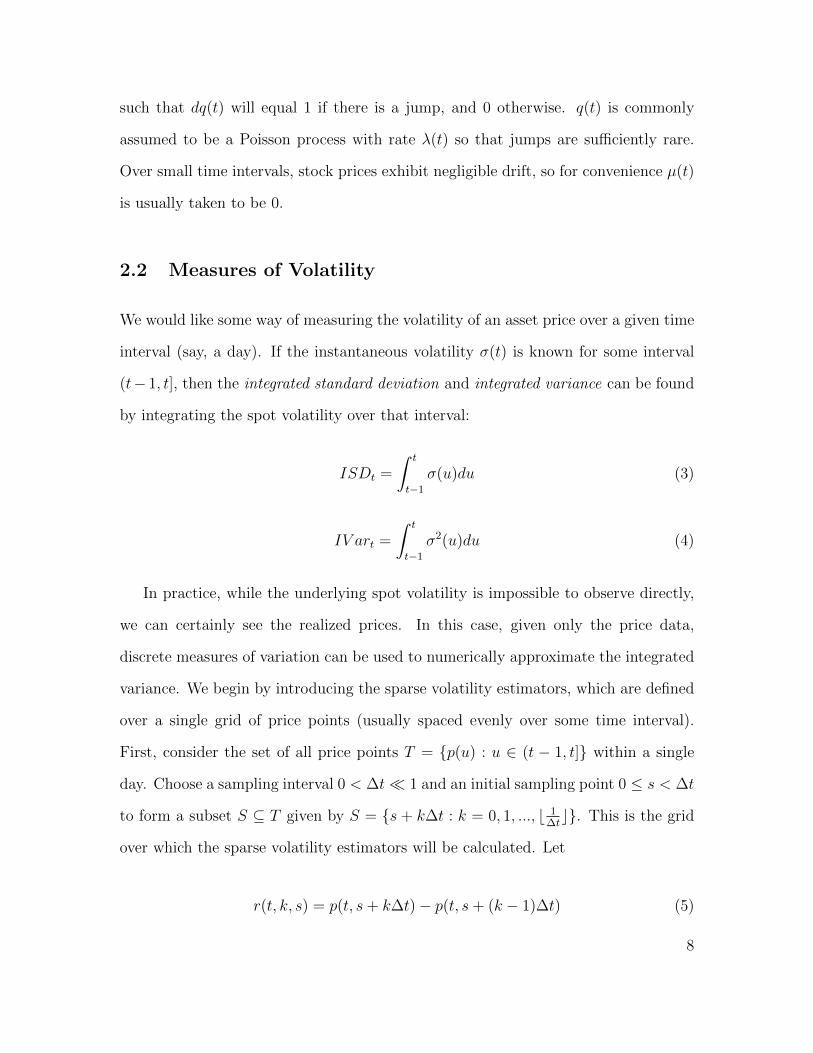
2.2 Measures of Volatility
We would like some way of measuring the volatility of an asset price over a given time
interval (say, a day). If the instantaneous volatility σ(t) is known for some interval
(t− 1, t], then the integrated standard deviation and integrated variance can be found
by integrating the spot volatility over that interval:
ISDt =
∫ t
t−1
σ(u)du (3)
IV art =
∫ t
t−1
σ2(u)du (4)
In practice, while the underlying spot volatility is impossible to observe directly,
we can certainly see the realized prices. In this case, given only the price data,
discrete measures of variation can be used to numerically approximate the integrated
variance. We begin by introducing the sparse volatility estimators, which are defined
over a single grid of price points (usually spaced evenly over some time interval).
First, consider the set of all price points T = {p(u) : u ∈ (t − 1, t]} within a single
day. Choose a sampling interval 0 < ∆t� 1 and an initial sampling point 0 ≤ s < ∆t
to form a subset S ⊆ T given by S = {s + k∆t : k = 0, 1, ..., b 1∆tc}. This is the grid
over which the sparse volatility estimators will be calculated. Let
r(t, k, s) = p(t, s+ k∆t)− p(t, s+ (k − 1)∆t) (5)
8

denote the kth logarithmic (geometric) return within day t, where p(t, s+ k∆t) is the
logarithm of the observed price at time s+ k∆t.
We are now ready to define the two different sparse volatility estimators, the
Realized Variance (RV) and the Realized Absolute Value (RAV). RV is simply the
quadratic variation of the log-return process, defined as the sum of the squared log-
returns, and RAV is the sum of the absolute value of the log-returns. Letting ∆t ∈
(0, 1] be our sampling interval, we calculate the daily sparse RV and RAV as follows:
RVt =
b1/∆tc∑k=1
r2(t, k, s)∆t→0−→
∫ t
t−1
σ2(u)du+∑
{u∈(t−1,t] : dq(u)=1}
κ2(u) (6)
RAVt =
√π
2
b1/∆tc∑k=1
|r(t, k, s)| ∆t→0−→∫ t
t−1
σ(u)du (7)
Observe that in the presence of jumps (and the absence of noise), the RV estima-
tor should converge asymptotically to the integrated variance plus the sum of the
jump values, while the RAV estimator converges to the integrated standard devia-
tion. Huang and Tauchen (2005) find that, on average, the jump component accounts
for roughly 5 to 7 percent of the total daily variance in the S&P500. It is reasonable,
then, to choose the realized variance as an appropriate estimator of the integrated
variance, even in the presence of jumps.
Following the work of Zhang, Mykland and Aıt-Sahalia (2005), we will also look at
the properties of sub-sampled realized variance. As before, given a sampling interval
∆t and n initial sampling points 0 ≤ s1 < s2 < ... < sn < ∆t, we can partition the
time periods in each day into grids Si = {si + k∆t : k = 0, 1, ...,mi}, where mi is the
total number of returns taken in a day starting from point si. Naturally, we require
that 1 − ∆t < si + mi∆t ≤ 1. Let r(t, k, i) = p(t, si + k∆t) − p(t, si + (k − 1)∆t).
9

From this, define RV(i)t as the RV on day t estimated over the grid Si:
RV(i)t =
mi∑k=1
r2(t, k, i) (8)
The sub-sampled realized variance, RV SSt , is the average of the RV
(i)t :
RV SSt =
1
n
n∑i=1
RV(i)t (9)
Then, the sub-sampled RAV is defined analogously:
RAV SSt =
1
n
n∑i=1
mi∑k=1
|r(t, k, i)| (10)
Note that for some si, mi = maxj {mj} − 1, so in those situations we apply a small
size-correction term defined by mi+1mi
.
2.3 Market Microstructure Noise and Volatility Estimation
In a perfectly efficient market, where stock prices adjust instantaneously to new in-
formation, the price of a stock at any point in time should be equal to the sum of all
future dividends (or earnings), discounted at an appropriate rate. In reality, owing
to various market frictions, the markets cannot move synchronously with the ideal
price. The market microstructure noise ε(t) is modeled as a noise term representing
the difference between the efficient log-price p(t) and the observed log-price p(t):
p(t) = p(t) + ε(t) (11)
10

While noise can come from a variety of sources, two of the most important sources
are the bid-ask bounce and the discontinuity of price changes. The bid-ask bounce
is a phenomenon wherein prices may bounce around between ask prices and bid
prices as traders buy and sell stocks without there being any actual change in the
fundamental valuation of the stock. The discontinuity of price changes refers to the
fact that prices are given in fixed increments, or ‘tick sizes’, so price movements are
inherently discontinuous. For example, in the United States, prices must move in
integer multiples of one cent - trades involving fractions of cents are not allowed. It
should be noted that market microstructure noise includes only short term deviations
from the efficient price. In the study of high-frequency data, secular fluctuations,
which generally arise from behavioral phenomena such as ‘irrational exuberance’, can
generally be treated as higher order effects and consequently ignored.
Market microstructure noise is extremely problematic because theoretically, as
the sampling interval decreases to 0, we should be able to obtain arbitrarily accurate
estimates of the integrated volatility. However, for small ∆t, the realized variance
estimators will be severely biased by market microstructure noise. We can think about
this in the following way. Since p(t) is continuous, p(t + ∆t) − p(t) → 0 as ∆t → 0.
However, because ε(t) is discontinuous and nonzero almost surely, ε(t+∆t)−ε(t) 9 0.
Therefore, as we decrease the sampling interval (letting ∆t→ 0), the change in p(t) is
increasingly dominated by the differences in the noise term. Continuing along this line
of thought, Bandi and Russell (2008) show that in the presence of independent and
identically distributed noise, the RV estimator will diverge to infinity almost surely
as ∆t → 0. This is problematic because letting ∆t become too large decreases the
accuracy of the approximations.
In Figure 2, we show the volatility signature plots of both the sparse RV and RAV
11

and the sub-sampled RV and RAV. The volatility signature plot is a tool introduced
by Andersen, Bollerslev, Diebold, and Labys (1999). Essentially, the volatility signa-
ture plot looks at the relationship between the average volatility calculated for each
different sampling interval. The x-axis shows the sampling interval ∆t, and the y-axis
shows the average calculated volatility for that particular sampling interval. In the
absence of noise, the volatility signature plot should look like a flat line, since noise
will no longer bias the estimates. In our data, notice that for ∆t > 5 min, the volatil-
ity signature plot is relatively stable for both RV and RAV. Below 5 minutes, both
measures drop dramatically as ∆t→ 0. This implies that for small ∆t, the volatility
estimators are significantly impacted by market microstructure noise. Therefore, in
practice returns are usually sampled at an interval which seeks to balance accuracy
versus robustness. There is a large body of literature which seeks to determine the
sampling interval which can best optimize that balance; for most applications, it suf-
fices to heuristically determine the optimal sampling interval based on the volatility
signature plot.
The obvious advantage of sub-sampling is that it allows us to make better use
of the available data while preserving the robustness of an appropriately-sampled
sparse RV. The sub-sampled RV estimator therefore improves on the basic sparse RV
estimator, but the algorithm is slightly more computationally expensive to implement.
3 Statistical Methodology
3.1 HAR Regression Models
In this paper, we rely on the Heterogeneous Autoregressive (HAR) models first in-
troduced by Corsi (2003) and Muller et. al. (2007) to forecast volatility. A key
12

property of market volatility is that it exhibits the long memory property, meaning
that volatility tends to be autocorrelated even for high lag values; more informally,
it implies that the value of a market’s volatility today will tend to correlate with
its volatility well into the future. Naturally, we would like our models to be able
to capture this feature. One way to incorporate long memory into the model is to
use fractional integration, such as an autoregressive fractionally integrated moving
average (ARFIMA) model, or the fractionally integrated generalized autoregressive
conditional heteroskedasticity (FIGARCH) model introduced by Baillie, Bollerslev,
and Mikkelsen (1996). While these models are relatively parsimonious, their ma-
jor drawback is that they are difficult to estimate, requiring complicated nonlinear
maximum likelihood-type estimation procedures. However, recent papers (see: An-
dersen, Bollerslev, Diebold, and Labys (2003) or Andersen, Bollerslev, and Huang
(2007)) have shown empirically that simple linear models can often predict future
volatility more accurately than the more sophisticated models such as FIGARCH
and ARFIMA. Corsi’s HAR model is one such formulation; by describing future
volatility as a linear combination of historical volatilities at a few choice time scales,
it captures a portion of the persistence effects in a parsimonious way, and it has the
major advantage of being easily estimated using simple OLS procedures.
In order to estimate a HAR model, first define RVt,t+h as the average RV over a
given time span h.
RVt,t+h =1
h
t+h∑k=t+1
RVk (12)
RAVt,t+h is then defined analogously. In this paper, we choose to estimate 22-day
ahead forecasts, which correspond to the number of trading days within a calendar
month, as well as the forecast horizon of the VIX index (a measure of market-implied
volatility, see the next subsection for a slightly more detailed explanation).
13

The basic form of the HAR-RV model is given by
RVt,t+22 = α + β1RVt−1,t + β5RVt−5,t + β22RVt−22,t + εt+1 (13)
where the dependent variables correspond to daily, weekly, and monthly lagged re-
gressors, which were chosen by Corsi in his paper.
Forsberg and Ghysels (2007) extend the HAR-class models by using historical
RAV to forecast future RV, which they find to be a significantly better predictor of
RV than historical RV. The model is analogous to the one for HAR-RV, and is defined
as:
RVt,t+22 = α + β1RAVt−1,t + β5RAVt−5,t + β22RAVt−22,t + εt+1 (14)
It should be noted that the physical interpretation of the HAR-RAV model differs
from the HAR-RV model, since RAV and RV are in different units. However, note that
both models seek to predict future volatility in RV units, allowing a direct comparison
of the empirical results.
Recall that the stochastic differential equation modeling stock price movements
included a jump term, κ(t)dq(t). There is an entire body of literature devoted to
studying these jumps as they relate to volatility estimation. However, Andersen,
Bollerslev, and Diebold (2007) studied an extension of the HAR model which incor-
porated terms modeling jump components into the regression. What they found was
that in general, the jump effects embedded in RV measures are not significant within
the context of HAR regressions. For this reason, we will only look at the basic HAR
models that do not incorporate jump effects.
14
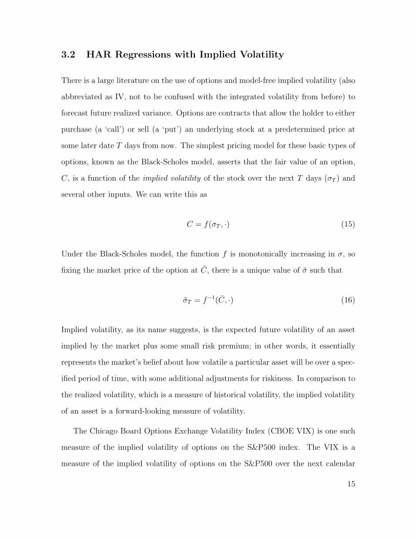
3.2 HAR Regressions with Implied Volatility
There is a large literature on the use of options and model-free implied volatility (also
abbreviated as IV, not to be confused with the integrated volatility from before) to
forecast future realized variance. Options are contracts that allow the holder to either
purchase (a ‘call’) or sell (a ‘put’) an underlying stock at a predetermined price at
some later date T days from now. The simplest pricing model for these basic types of
options, known as the Black-Scholes model, asserts that the fair value of an option,
C, is a function of the implied volatility of the stock over the next T days (σT ) and
several other inputs. We can write this as
C = f(σT , ·) (15)
Under the Black-Scholes model, the function f is monotonically increasing in σ, so
fixing the market price of the option at C, there is a unique value of σ such that
σT = f−1(C, ·) (16)
Implied volatility, as its name suggests, is the expected future volatility of an asset
implied by the market plus some small risk premium; in other words, it essentially
represents the market’s belief about how volatile a particular asset will be over a spec-
ified period of time, with some additional adjustments for riskiness. In comparison to
the realized volatility, which is a measure of historical volatility, the implied volatility
of an asset is a forward-looking measure of volatility.
The Chicago Board Options Exchange Volatility Index (CBOE VIX) is one such
measure of the implied volatility of options on the S&P500 index. The VIX is a
measure of the implied volatility of options on the S&P500 over the next calendar
15

month (30 days). The values of the VIX are derived, in real time, from a range of
calls and puts on the S&P500 set to expire in one or two months. In 2003, the CBOE
changed how it calculated the VIX, abandoning options-implied volatility in favor of
model-free implied volatility. Jiang and Tian (2005) showed that model-free implied
volatility is better than options-implied volatility at predicting future volatility and
endorsed the CBOE’s switch to a nonparametric framework for estimating implied
volatility.
Poon and Granger (2005) and a literature review by Blair, Poon, and Taylor (2001)
conclude that implied volatility is a better predictor of volatility than the commonly
used time-series models. Mincer and Zarnowitz (1969) proposed a simple framework
with which to evaluate the efficiency of implied volatility-based forecasting:
RVt,t+22 = α + βIV IVt + εt+1 (17)
If implied volatility were perfectly efficient, then α = 0 and βIV = 1. However,
numerous papers, including Becker, Clements, and White (2003), find that this is not
the case.
Fradkin (2008) found evidence that adding implied volatility to HAR models al-
most always improved model fit, which suggests that implied volatility contains in-
formation not present in historical volatility. We will define hybrid HAR-RV-IV and
HAR-RAV-IV models identical to those used by Fradkin:
RVt,t+22 = α + β1RVt−1,t + β5RVt−5,t + β22RVt−22,t + βIV IVt + εt+1 (18)
RVt,t+22 = α + β1RAVt−1,t + β5RAVt−5,t + β22RAVt−22,t + βIV IVt + εt+1 (19)
16
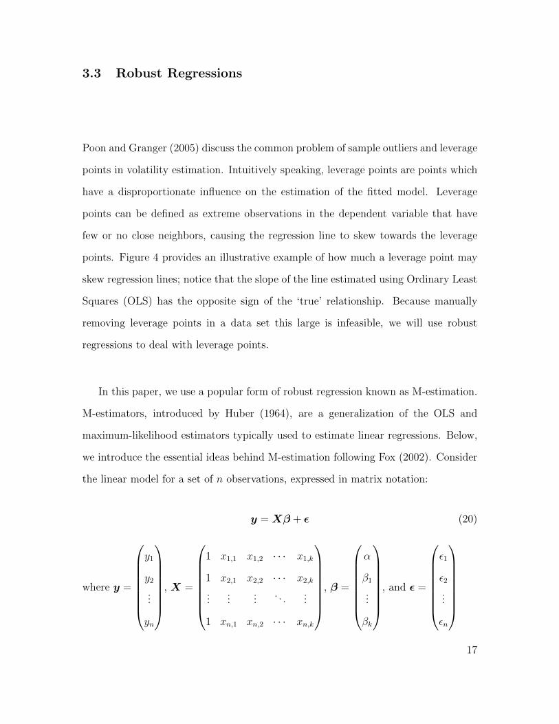
3.3 Robust Regressions
Poon and Granger (2005) discuss the common problem of sample outliers and leverage
points in volatility estimation. Intuitively speaking, leverage points are points which
have a disproportionate influence on the estimation of the fitted model. Leverage
points can be defined as extreme observations in the dependent variable that have
few or no close neighbors, causing the regression line to skew towards the leverage
points. Figure 4 provides an illustrative example of how much a leverage point may
skew regression lines; notice that the slope of the line estimated using Ordinary Least
Squares (OLS) has the opposite sign of the ‘true’ relationship. Because manually
removing leverage points in a data set this large is infeasible, we will use robust
regressions to deal with leverage points.
In this paper, we use a popular form of robust regression known as M-estimation.
M-estimators, introduced by Huber (1964), are a generalization of the OLS and
maximum-likelihood estimators typically used to estimate linear regressions. Below,
we introduce the essential ideas behind M-estimation following Fox (2002). Consider
the linear model for a set of n observations, expressed in matrix notation:
y = Xβ + ε (20)
where y =
y1
y2
...
yn
, X =
1 x1,1 x1,2 · · · x1,k
1 x2,1 x2,2 · · · x2,k
......
.... . .
...
1 xn,1 xn,2 · · · xn,k
, β =
α
β1
...
βk
, and ε =
ε1
ε2...
εn
17

and the corresponding fitted model
y = Xb+ r (21)
One property of regressions is that they fit values at the ends of the data better
than values in the middle. As a result, they will yield different residual distributions
at different points, even if the true error terms are identically distributed, making
comparisons between the residuals of different points impossible. This fact motivates
the practice of studentizing the residuals, a way of norming the residuals analogous
to standardizing a random variable. Given a residual ri = yi − yi, an appropriate
estimate of its standard deviation σ, and its leverage hii, the studentized residual ei
is given by:
ei =ri
σ√
1− hii(22)
The value of hii is a measure of the leverage of the ith data point. It is given by the iith
entry along the diagonal of the hat matrix H = X(XTX)−1XT . One common way to
estimate σ is to use the Median Absolute Deviation (MAD), a more robust measure
of spread than the standard deviation. The MAD is defined as the median of the
absolute deviations from the median of the data, i.e., for some set U = {u1, u2, ..., un}
with median υ,
MAD = mediani{|ui − υ|} (23)
σ = c×MAD (24)
For a symmetric distribution about the mean, the MAD will be the equal to the
3rd quartile. In the case of the standard normal distribution, the MAD must be
divided by the inverse normal cumulative distribution function evaluated at 34, or
18

Φ−1(34) ≈ 0.6745. We can then choose c = 1
0.6745≈ 1.4826 so that σ is unbiased for
normally distributed errors.
The goal of the M-estimator is to find a (unique) solution b that minimizes an
objective function:
b = minb
n∑i=1
ρ(ri) (25)
where ri = yi − yi is the residual of point i and ρ(r) is a penalty function giving the
contribution of each residual to the overall objective function.
By definition of r, ρ(r) is a function of the parameters in b, so for any continuously
differentiable function ρ, we can take the partial derivatives of ρ(r) with respect to
each of the parameters in b and set them to 0, producing a system of k + 1 linear
equations. Taking the derivative of ρ(r) with respect to e yields the influence function
ψ(r) = ρ′(r), the system of equations can be written as the vector equation:
n∑i=1
ψ(ri)xTi = 0 (26)
Now, define a weight function w(r) such that w(r)r = ψ(r), so the system we would
like to solve becomes:n∑i=1
w(ri)rixTi = 0 (27)
Notice that in order to solve the system of linear equations, we need to know the
residuals, which depend on the fitted regression, which in turn depends on the weights.
Therefore, the system must be solved iteratively. We use an Iteratively Reweighted
Least Squares (IRLS) algorithm, which begins by obtaining an initial model estimate
b(0) using OLS. At each iteration, we calculate a new set of residuals and weights
based on the previous iteration’s parameter estimates. Then, the new weighted least
squares estimates can be solved for. The previous two steps are repeated until the
19
estimates for b converge.
The choice of ρ(r) determines the robustness of the estimator b to leverage points.
Intuitively, a sensible choice for ρ(r) should be one such that points above the fitted
line are just as important as points below the line, any deviation from the fitted
line incurs a penalty, and larger deviations will not be penalized less than smaller
ones. Mathematically, we require that ρ(r) be symmetric about 0, positive definite,
and non-decreasing in |r|. For the OLS estimator, ρ(r) = r2, so that the estimate
b minimizes the sum of the squared residuals, as expected. The influence function
ψ(r) = 2r is linear in the residual; a problem for OLS estimators is that, as the
residual increases, the influence of that point also increases without bound. The
weight function is w(r) = 1, implying that all points are given equal weighting.
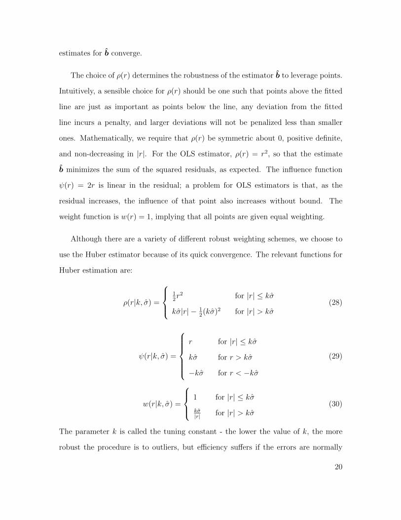
Although there are a variety of different robust weighting schemes, we choose to
use the Huber estimator because of its quick convergence. The relevant functions for
Huber estimation are:
ρ(r|k, σ) =
12r2 for |r| ≤ kσ
kσ|r| − 12(kσ)2 for |r| > kσ
(28)
ψ(r|k, σ) =
r for |r| ≤ kσ
kσ for r > kσ
−kσ for r < −kσ
(29)
w(r|k, σ) =
1 for |r| ≤ kσ
kσ|r| for |r| > kσ
(30)
The parameter k is called the tuning constant - the lower the value of k, the more
robust the procedure is to outliers, but efficiency suffers if the errors are normally
20

distributed. The value of k is often set at 1.345 so that the IRLS algorithm provides
approximately 95% efficiency if errors are normal. It is not difficult to see why the
Huber estimator is more robust than OLS. Although the Huber estimator is identical
to the OLS estimator when the residuals are within a certain range determined by the
tuning constant, after that point, larger residuals are assigned ever smaller weights.
Similarly, looking at the influence function, the Huber estimator bounds the influence
of any point at±kσ. Figure 5 shows a comparison of the penalty, influence, and weight
functions for the OLS estimator and the Huber estimator. In Matlab, the residuals
are studentized first, so σ can be taken as 1 and r = e will be the studentized residual.
3.4 Evaluating Regression Performance
There are a number of different methods for evaluation forecast accuracy. This paper
uses Mean Absolute Percentage Error (MAPE) because it is a scale-free and robust
measure of relative accuracy, allowing us to compare results over different levels of
RV. Letting yi be the fitted value for point i, and yi be the actual value, we define
MAPE as:
MAPE =1
n
n∑i=1
| yi − yiyi| (31)
The main concern with MAPE is that because the measure is not upper-bounded, we
must be careful of very small or zero values for yi. As Figure 3 shows, the RV values
used for the denominator are reasonably far away from 0, so this should not be much
of an issue.
21

4 Data and Methods
4.1 Data Preparation
The high-frequency stock price data used in this paper were obtained from an online
vendor, price-data.com. For each trading day, the prices from the first 5 minutes of
the day were discarded, leaving a total of 385 price samples which run from 9:35AM
to 4:00PM. For this paper, we follow Law (2007) and select 40 of the largest market
capitalized stocks from the S&P100 (OEX) and aggregate those stocks to form a
portfolio that we claim can proxy for the S&P500 (SPX) for two reasons: the OEX
is a subset of the SPX, and the two indices are highly correlated. Our requirement
for inclusion was that data for the stock be present from Jan. 3, 2000 up through
Dec. 31, 2008; we also checked for inconsistencies in the data and adjusted the prices
for stock splits. In creating the portfolio, we kept only the data for those days in
which all 40 stocks traded, yielding a total of 2240 days. We used an equal-weighting
scheme to construct our portfolio by ‘buying’ $25 of each stock at its initial price.
The implied volatility data was taken from the CBOE website. We used the VIX,
a model-free implied volatility index which uses a range of options on the SPX to
calculate the 1-month-ahead implied volatility for the S&P500. Because intra-day
data was not available, we only used the closing price of the VIX in our regressions.
We transformed the data into the same units as the realized variance.
Our in-sample data spans 7 years, from the beginning of 2000 until the end of
2006, yielding 1743 data points. Our out-of-sample data runs from the beginning of
2007 until the end of 2008, yielding 497 data points. We therefore have 24 indepen-
dent month-long periods for the out-of-sample result, which should be sufficient to
accurately gauge out-of-sample performance.
22

4.2 Analysis Methodology
For the volatility data, the sparse and sub-sampled estimators were calculated at every
sampling interval from 1 minute up to 30 minutes. In each regression, the historical
volatility sampled at j minutes were regressed against the 1-month-ahead volatility
sampled at k minutes for j and k between 1 and 30 minutes, meaning that a total of
900 regressions were run for each model. There are four models used in the paper:
the HAR-RV, the HAR-RV-IV, the HAR-RAV, and the HAR-RAV-IV. Each model
was estimated twice, once using OLS and once using the robust M-estimation. After
an initial training period on the in-sample data, the models were evaluated on out-of-
sample accuracy using the MAPE measure. We note that the estimated coefficients
in the regression models were not updated during the out-of-sample period. While
dynamic coefficients would likely be implemented when forecasting for real world
use, the general results from our simpler algorithm should still hold under the more
complex scheme.
5 Results
5.1 In-sample Fit
Figures 6 through 12 show graphs of the MAPE for each model specification plotted
against the LHS and RHS sampling intervals. When the sampling interval for either
side of the regression is small (∆t < 5 min), the in-sample surface plots show a
marked increase in what we will call the ‘variation in fit’ (abbreviated from now on
as ViF). By the ViF at a particular point, we mean the degree to which the model
fit responds to small changes in the model parameters (the size of the LHS and RHS
23

sampling intervals) around that point. This concept corresponds to the magnitude of
the gradient (or slope, depending on the context) of the MAPE surface curves. Above
this threshold, the surface plot is relatively flat, meaning that all models are roughly
equally adept at predicting future volatility. Sample fit increases when the left hand
side (LHS) sampling interval decreases in each of the models. For the HAR-RAV
models, fit decreases when the RHS sampling interval decreases.
The addition of implied volatility appears to offer uniformly significant improve-
ments to the all four of the HAR models (RV, RAV, RV-IV, and RAV-IV). This result
is consistent with previous studies showing that a large proportion of the informa-
tion contained in IV cannot be found in historical data. Sub-sampling eliminates
much of the noisiness in model fit; however, it does not improve fit uniformly across
all sampling intervals. Therefore, although using sub-sampling ensures some degree
of consistency in our results, it does not appear to play a major role in improving
accuracy. The robust regressions appear to offer a better fit for each of the four re-
gression models relative to their OLS-estimated counterparts. Moreover, the ViF is
substantially lower in the robustly-estimated models.
We report OLS coefficients for selected combinations for each model in Table 1
and robust coefficients in Table 2. The standard errors for the OLS coefficients are
Newey-West standard errors with a lag of 44 days. We find that in general, the
coefficients are significant at the α = 0.05 level or higher. The robust regression
coefficients are, with few exceptions, highly significant (p < 0.001); however, such
high t-scores are very likely a result of the standard errors not being robust to serial
correlations.
24

5.2 Out-of-sample Performance
From Figures 9-12, we see many of the same results that were discussed above. As
we found for the in-sample fit, the surface plots could be divided into two regions:
the high-ViF region (when either LHS or RHS was sampled below 5 min intervals)
and the stable region (when both LHS and RHS were sampled at above 5 min).
HAR-RV and HAR-RAV perform very similarly in the out-of-sample period. In
both models, there is significantly higher ViF with respect to the RHS compared to
the LHS. The inclusion of IV into our regressions reduces much of the ViF seen for
small ∆t on the RHS. Models estimated using the robust procedure, independent of
IV, produced the most accurate forecasts out-of-sample.
We should note that the out-of-sample period used in this paper encompasses a
period of unusually high volatility due to the recent economic turmoil, as seen in
Figure 3. Fradkin (2007) and Forsberg and Ghysels (2007) both found clear evidence
that HAR-RAV offered the best predictions of future volatility. However, they used
2005 and 2001-2003 as their out-of-sample periods, respectively, periods that were
both characterized by relatively low volatility. This may imply that HAR-RAV offers
a significant advantage over HAR-RV when the overall volatility is low and persistence
effects are not as strong.
5.3 Discussion
The empirical results, both in-sample and out-of-sample, paint a fairly coherent pic-
ture about the effects of market microstructure noise. In a world without market
microstructure noise, we should expect to find that the model fits are relatively ho-
mogeneous across LHS and RHS sampling intervals. In reality, we see that in the
25
base HAR-RV and HAR-RAV models, models whose sampling intervals were below
5 min showed a high ViF, which implies that market microstructure noise becomes
first order when the prices are sampled once every 5 or fewer minutes. The relative
homogeneity in model fit for sampling intervals between 5 to 30 minutes suggests
that the information content of these volatility measures do not change much in this
range.
If implied volatility is added into the regressions, a large portion of the high-
frequency ViF is eliminated for both the RV and RAV models. This suggests that the
new information contained in IV can swamp the distortionary effects of the market
microstructure noise. Implementing robust regressions also reduced the effects of
market microstructure noise, but by a smaller factor than implied volatility. When
both implied volatility and robust regressions are used, the ViF at the high-frequencies
virtually disappears. This result implies that there are ways to compensate for the
market microstructure noise to the point where it is no longer inadvisable to sample
at very high frequencies.
We also find that sub-sampling does not actually improve accuracy by a significant
amount, although for the larger sampling intervals it does eliminate much of the
noisiness in the estimates, allowing forecasts to be consistent across different sampling
interval combinations. Because the sub-sampled volatility estimators in this paper
are set up so that all of the data points are used, all of the volatility estimates contain
the same information, so this result should not be surprising.
Since the general shape of the accuracy/fit surface plots stayed roughly the same
in the in-sample and out-of-sample periods, it suggests the presence of underlying
relationships in historical volatilities that remain fairly consistent over time. As for
the structure itself, referring back to Figure 2, observe that the average value of the
26

estimated RV’s increases dramatically for sampling intervals running from 1 min to
5 min, and then gradually tapers down as the sampling interval increases above 5
minutes. The ViF could be explained by the statistical properties of the data if, as
we posit above, the historical autocorrelations between volatility levels are relatively
consistent. In that case, we might expect that explanatory variables with higher
variances are better predictors than explanatory variables with lower variances. In our
study, when the historical variables are sampled below 5 min (low variability relative
to the future volatility variable), we find that the models perform significantly worse
relative to the stable region; when the future volatility variable is sampled below 5
min (more variation in the historical variables relative to the future volatility), we see
that the forecasts are more accurate relative to the stable region.
Although it is not directly related to the goals of the paper, the performance of the
robust regressions merits further discussion. Fradkin (2008) also found that robust
regressions were superior to OLS regression out-of-sample; however, his out-of-sample
period was 2005, which was a particularly calm year for the markets. The fact that the
robust regressions continued to perform well relative to the OLS regressions during
the tumultuous 2008 year suggests that much of the historical covariances from before
2008 have persisted in spite of the financial crisis in the latter half of 2008.
6 Conclusion
This paper investigated the relationship between market microstructure noise and
volatility forecasting by varying the frequency with which we sampled the high-
frequency data. We used both the naive sampling scheme and the more sophisti-
cated sub-sampling scheme to estimate the volatility. The regression models we used
27

were based on Corsi’s HAR model (2003); in total, four models - the HAR-RV, HAR-
RAV, HAR-RV-IV, and HAR-RAV-IV - were tested, along with both OLS and robust
estimation procedures.
We find that market microstructure noise has a significant distortionary effect
on the accuracy of volatility forecasts as we tighten the sampling interval. This is
especially true in the base cases, where the only explanatory variables are histor-
ical realized volatilities. The sub-sampled volatility estimators did not reduce the
high-frequency ViF, although it did reduce the noisiness of the RV estimator as we
increased the sampling interval. We also looked at regression methodology, comparing
OLS and robust procedures. In our data, robust regressions were found to mitigate
a large proportion of the ViF at high-frequencies. The third feature we incorporated
was the use of implied volatility, which was also found to improve consistency in fore-
cast accuracy. A combination of implied volatility and robust regressions was shown
to have made the forecasting models robust to market microstructure noise, suggest-
ing that for volatility forecasting, it may be possible to sample at extremely high
frequencies without having to worry about the noisiness. Thus, for the risk manager,
we recommend using a combination of implied volatility and robust regressions in
order to produce the most accurate and consistent volatility forecasts.
28

7 Appendix: Tables and Figures
Table 1: Coefficients for Select OLS Regressions (w/ Sub-sampling)
Coeff HAR-RV HAR-RAV HAR-RV-IV HAR-RAV-IV(1,1) (10,10) (1,1) (10,10) (1,1) (10,10) (1,1) (10,10)
β1 0.19*** 0.11** 0.004*** 0.004*** 0.11** 0.06* 0.003** 0.003**β5 0.37*** 0.27*** 0.008** 0.01*** 0.32** 0.22** 0.007** 0.009**β22 – 0.25** – – – – – –βIV n/a n/a n/a n/a 0.11** 0.22** 0.09* –
Coeff HAR-RV HAR-RAV HAR-RV-IV HAR-RAV-IV(10,1) (1,10) (10,1) (1,10) (10,1) (1,10) (10,1) (1,10)
β1 0.34*** 0.06** 0.01*** 0.002*** 0.17* 0.03* 0.004* 0.001*β5 0.64** 0.15*** 0.01** 0.01*** 0.53** 0.12** 0.01* 0.004**β22 – 0.21*** – 0.003* – – – –βIV n/a n/a n/a n/a 0.24*** 0.14*** 0.18** –
Table 2: Coefficients for Select Robust Regressions (w/ Sub-sampling)
Coeff HAR-RV HAR-RAV HAR-RV-IV HAR-RAV-IV(1,1) (10,10) (1,1) (10,10) (1,1) (10,10) (1,1) (10,10)
β1 0.18*** 0.12*** 0.003*** 0.003*** 0.11*** 0.06*** 0.002*** 0.002***β5 0.30*** 0.27*** 0.01*** 0.01*** 0.25*** 0.18*** 0.005*** 0.01***β22 0.21*** 0.21*** 0.003*** 0.004*** 0.10*** 0.05*** 0.002*** 0.001***βIV n/a n/a n/a n/a 0.08*** 0.17*** 0.08*** 0.11***
Coeff HAR-RV HAR-RAV HAR-RV-IV HAR-RAV-IV(10,1) (1,10) (10,1) (1,10) (10,1) (1,10) (10,1) (1,10)
β1 0.30*** 0.08*** 0.005*** 0.002*** 0.12*** 0.04*** 0.002*** 0.001***β5 0.37*** 0.15*** 0.01*** 0.004*** 0.28*** 0.10*** 0.01*** 0.003***β22 0.27*** 0.17*** 0.004*** 0.003*** -0.01 0.08*** – 0.07***βIV n/a n/a n/a n/a 0.19*** 0.11*** 0.17*** 0.07***
Tables 1 and 2 show the results of a select number of OLS regressions. Each pair(Left, Right) denotes the sampling interval of the regression’s left hand side (the de-pendent variable) and the sampling interval used on the right hand side (explanatoryvariables). The significance levels of the coefficients are denoted by the asterisks:∗ =⇒ p<0.05, ∗∗ =⇒ p<0.01, ∗ ∗ ∗ =⇒ p<0.001
Finally, the OLS standard errors were calculated using Newey-West standard er-rors with lag length 44. The robust regressions used heteroskedasticity-robust stan-dard errors.
29

Figure 1: Intra-day Price Movements for Two Randomly Selected Days
Figure 2: Volatility Signature Plots
30
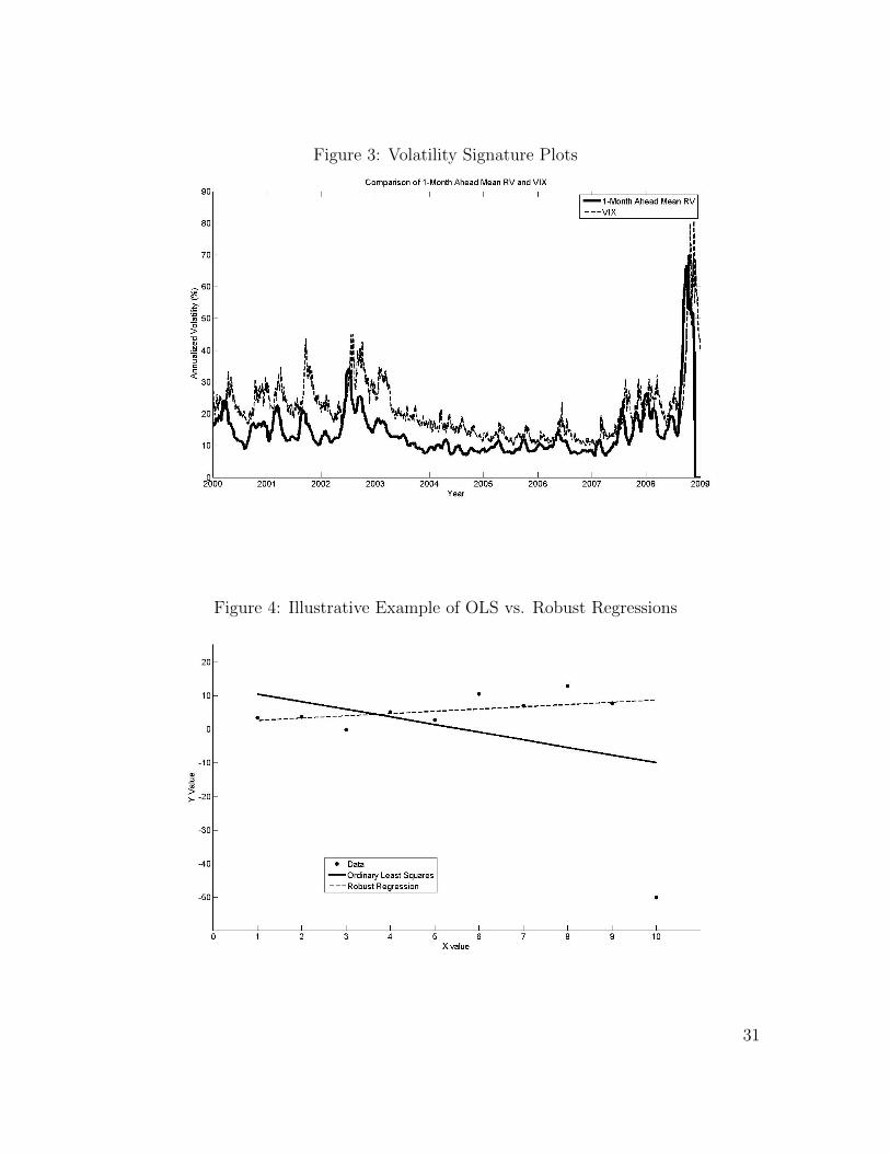
Figure 3: Volatility Signature Plots
Figure 4: Illustrative Example of OLS vs. Robust Regressions
31
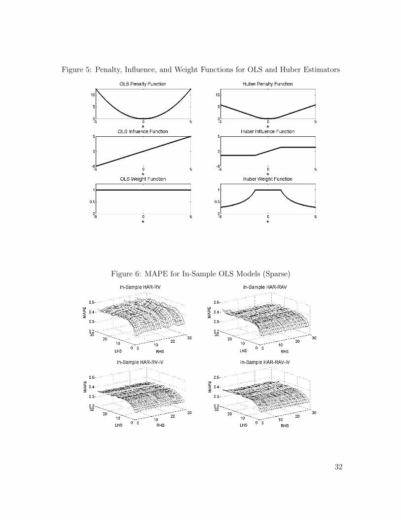
Figure 5: Penalty, Influence, and Weight Functions for OLS and Huber Estimators
Figure 6: MAPE for In-Sample OLS Models (Sparse)
32

Figure 7: MAPE for In-Sample OLS Models (Sub-Sampling)
Figure 8: MAPE for In-Sample Robust Models (Sub-Sampling)
33
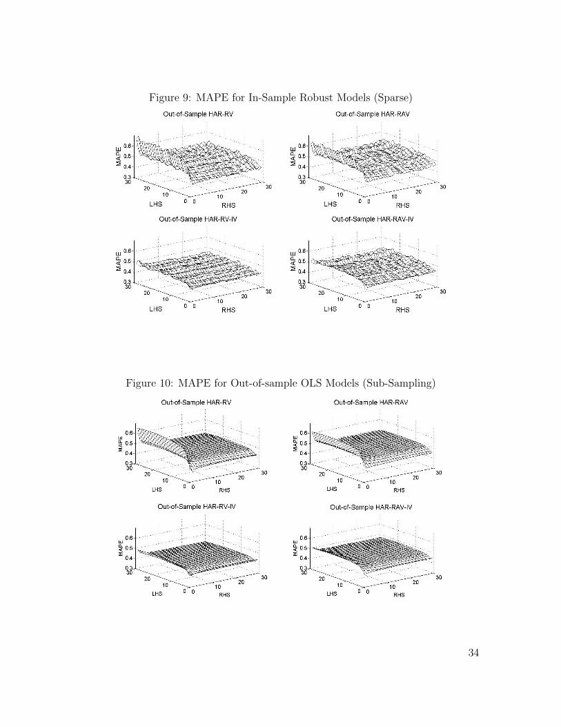
Figure 9: MAPE for In-Sample Robust Models (Sparse)
Figure 10: MAPE for Out-of-sample OLS Models (Sub-Sampling)
34

Figure 11: MAPE for Out-of-Sample Robust Models (Sparse)
Figure 12: MAPE for Out-of-sample Robust Models (Sub-Sampling)
35

References
[1] Aıt-Sahalia, Y. and Yu, J. (2009). High Frequency Market Microstructure NoiseEstimates and Liquidity Measures. The Annals of Applied Statistics, 3(1), 422-457.
[2] Andersen, T., Bollerslev, T., and Diebold F. (2007). Roughing It Up: IncludingJump Components in the Measurement, Modeling, and Forecasting of ReturnVolatility. The Review of Economics and Statistics, 89(4), 701-720.
[3] Andersen, T., Bollerslev, T. (1998). Answering the Skeptics: Yes, StandardVolatility Models Do Provide Accurate Forecasts. International Economic Re-view, 39(4), 885-905.
[4] Andersen, T., Bollerslev, T., Diebold, F., and Labys, P. (1999). Realized Volatil-ity and Correlation. Working Paper, Northwestern University.
[5] Andersen, T., Bollerslev, T., Diebold, F., and Labys, P. (2003). Modeling andForecasting Realized Volatility. Econometrica, 71(2), 579-625.
[6] Andersen, T., Bollerslev, T., and Huang, X. (2007). A Semiparametric Frame-work for Modeling and Forecasting Jumps and Volatility in Speculative Prices.Working Paper, Duke University.
[7] Andersen, T., Bollerslev, T., and Meddahi, N. (2007). Realized Volatility Fore-casting and Market Microstructure Noise. Working Paper, Northwestern Univer-sity.
[8] Baillie, R., Bollerslev, T., and Mikkelsen, H. (1996). Fractionally Integrated Gen-eralized Autoregressive Conditional Heteroskedasticity. Journal of Econometrics,74(1), 3-30.
[9] Bandi, F. and Russell, J. (2008). Microstructure Noise, Realized Variance, andOptimal Sampling. Review of Economic Studies, 75(2), 339-369.
[10] Becker, R., Clements, A., and White, S. (2006). On the Informational Efficiencyof S&P500 Implied Volatility. North American Journal of Economics and Fi-nance, 17(2), 139-153.
[11] Blair, B., Poon, S-H., and Taylor, S. (2001). Forecasting SP100 Volatility: TheIncremental Information Content of Implied Volatilities and High-Frequency In-dex Returns. Journal of Econometrics, 105(1), 5-26.
[12] Corsi, F. (2003). A Simple Long Memory Model of Realized Volatility. Unpub-lished manuscript, University of Logano.
36

[13] Forsberg, L. and Ghysels, E. (2007). Why do Absolute Returns Predict VolatilitySo Well? Journal of Financial Econometrics, 5(1), 31-67.
[14] Fradkin, A. (2007). The Informational Content of Implied Volatility in IndividualStocks and the Market. Unpublished manuscript, Duke University.
[15] Fox, J. (2002). Robust Regression. Available online at http://cran.r-project.org/doc/contrib/Fox-Companion/appendix-robust-regression.pdf.
[16] Huang, X. and Tauchen, G. (2005). The Relative Contribution of Jumps to TotalPrice Variance. Journal of Financial Econometrics, 3(4), 456-499.
[17] Huber, P. (1964). Robust Estimation of a Location Parameter. The Annals ofMathematical Statistics, 35(1), 73-101.
[18] Jiang, G. and Tian, Y. (2005). The Model-Free Implied Volatility and its Infor-mational Content. Review of Financial Studies, 18(4), 1305-1342.
[19] Law, T.H. (2007). The Elusiveness of Systematic Jumps. Unpublishedmanuscript, Duke University.
[20] Merton, R. C. (1971). Optimum Consumption and Portfolio Rules in aContinuous-Time Model. Journal of Economic Theory, 3, 373-413.
[21] Merton, R. C. (1976). Option Pricing When Underlying Stock Returns are Dis-continuous. Journal of Financial Economics, 3, 125-144.
[22] Mincer, J. and Zaronwitz, V. (1969). The Evaluation of Economic Forecasts, inJ. Mincer, ed., “Economic Forecasts and Expectations.” NBER, New York.
[23] Muller, U. A., Dacorogna, M.M., Dave, R. D., Olsen, R. B., Pictet, O.V., and vonWeizsacker, J. E. (1997). Volatilities of Different Time Resolutions - AnalyzingThe Dynamics of Market Components. Journal of Empirical Finance, 4, 213-239.
[24] Poon, S-H and Granger, C. (2005). Practical Issues in Forecasting Volatility.Financial Analysts Journal, 61(1), 45-56.
[25] Zhang, L., Mykland, L., and Aıt-Sahalia, Y. (2005). A Tale of Two Time Scales:Determining Integrated Volatility with Noisy High-Frequency Data. Journal ofthe American Statistical Association, 100, 1394-1411.
37