Embed Size (px)
Citation preview

Banco de Mexico
Documentos de Investigacion
Banco de Mexico
Working Papers
N◦ 2006-04
Volatility Forecasts for the Mexican Peso - U.S. DollarExchange Rate: An Empirical Analysis of GARCH,Option Implied and Composite Forecast Models
Guillermo BenavidesBanco de Mexico
April 2006
La serie de Documentos de Investigacion del Banco de Mexico divulga resultados preliminares detrabajos de investigacion economica realizados en el Banco de Mexico con la finalidad de propiciarel intercambio y debate de ideas. El contenido de los Documentos de Investigacion, ası como lasconclusiones que de ellos se derivan, son responsabilidad exclusiva de los autores y no reflejannecesariamente las del Banco de Mexico.
The Working Papers series of Banco de Mexico disseminates preliminary results of economicresearch conducted at Banco de Mexico in order to promote the exchange and debate of ideas. Theviews and conclusions presented in the Working Papers are exclusively the responsibility of theauthors and do not necessarily reflect those of Banco de Mexico.
Documento de Investigacion Working Paper2006-04 2006-04
Volatility Forecasts for the Mexican Peso - U.S. Dollar ExchangeRate: An Empirical Analysis of GARCH, Option Implied and
Composite Forecast Models*
Guillermo Benavides†
Banco de Mexico
AbstractThe volatility accuracy of several volatility forecast models is examined for the case of
daily spot returns for the Mexican peso - US Dollar exchange rate. The models applied areunivariate GARCH, a multi-variate GARCH (BEKK model), option implied volatilities, anda composite forecast model. The results show that the composite volatility forecasts are su-perior to the other models in terms of mean squared errors. Conclusions are as follows: thecomposite model is superior and both type of data -historical and implied in option pricesmust be used when available.Keywords: Composite forecast models, Exchange rates, Multivariate GARCH, Option im-plied volatility, Volatility forecasting.JEL Classification: C22, C52, C53, G10
ResumenEn el presente trabajo de investigacion se analiza el poder predictivo de varios mo-
delos de pronosticos de volatilidad diaria del tipo de cambio Peso Mexicano - Dolar Esta-dounidense. Los modelos que se utilizan son: univariado GARCH; multi-variado GARCH(modelo BEKK); volatilidad implıcita de opciones; y, un modelo compuesto. El modelo com-puesto fue el mas certero al compararlo con el resto de los modelos en terminos del errorcuadratico medio. Las conclusiones son: el modelo compuesto fue superior al pronosticary se deben de utilizar ambos tipos de datos -series historicas y de volatilidad implıcita deopciones- en especial si estos ultimos estan disponibles.Palabras Clave: Modelos de pronosticos compuestos, Multivariado GARCH, Pronosticosde volatilidad, Tipo de cambio peso - dolar, Volatilidad implıcita de opciones.
*I want to thank Alejandro Dıaz de Leon for valuable comments of an earlier version of this paper. I alsowant to thank Alfonso Guerra and participants at Banco de Mexico, and participants at the InternationalFinance Conference 2005 held at the University of Copenhagen in Denmark for useful comments and dis-cussion. Special thanks to Israel Mora for helpful programming advice and Luis Rodrıguez for providing thedata. Finally, I appreciate the very helpful suggestions from an anonymous referee.
† Direccion General de Investigacion Economica. Email: [email protected].
Contents
I. Introduction........................................................................................................... 1 II. Academic literature of volatility forecast models.................................................. 3
II.1. Arch-type volatility models ............................................................................ 3 II.2. Option implied volatility models..................................................................... 4 II.3. Composite forecast models .......................................................................... 6
III. Motivation ........................................................................................................... 7 IV. Contribution........................................................................................................ 8 V. The models ......................................................................................................... 9
V.1. Arch-type volatility models............................................................................ 9 V.2. Option implied volatility............................................................................... 16 V.3. The composite forecast model ................................................................... 16
VI. Data ................................................................................................................. 20
VI.1. Options and spot data ............................................................................... 20 VII. Descriptive statistics........................................................................................ 21 VIII. Results ........................................................................................................... 22
VIII.1. In-sample evaluation ............................................................................... 22 VIII.2. Out-of-sample evaluation ........................................................................ 23 VIII.3. Analysis of the results.............................................................................. 24
IX. Conclusion ....................................................................................................... 25 Bibliography........................................................................................................... 27 Appendix ............................................................................................................... 32
1
I. INTRODUCTION
There are basically four general methods widely used to forecast financial
volatility of financial variables. These are: 1) by using historical data (price returns),
2) by applying Autoregressive Conditional Heteroscedasticity - type models
(ARCH-type), 3) by calculating option implied volatilities (when option data is
available); and, 4) by using stochastic volatility models (Poon and Granger: 2003).1
By extrapolating the estimates of the different models it is possible to obtain
volatility forecasts. Even though all of these are widely used by academics and
practitioners, nowadays there is a current debate about which method is superior in
terms of forecasting accuracy (Brooks: 2002; Poon and Granger: 2003; Andersen
et al.: 2005).
The present paper addresses the existing debate in the academic literature
related to volatility forecasting accuracy by testing two of these methods: ARCH-
type and implied in options. In addition, a composite forecast specification will be
constructed with the volatility forecasts of the aforementioned methods. The main
objective is to analyze which forecast model is superior in terms of goodness-of-fit;
i.e., by comparing their mean squared errors (MSE). At present, there is no
individual method statistically proven to be the most accurate, although most of the
literature has found that option implieds are superior (Poon and Granger: 2003).
Everyday there is more research published on this topic. For example, by 2003,
1 Other methods to forecast financial volatility have been suggested. These are: Nonparametric, neural networks, genetic programming and models based upon time change and duration. However, it has been found that these have relatively less predictive power and the number of publications using these methods is substantially lower (Poon and Granger: 2003).

2
there were about one hundred working papers published (Andersen et al.: 2005;
Poon and Granger: 2003).
The models presented in this study are: 1) a univariate Generalized
Autoregressive Conditional Heteroskedasticity (GARCH) model (Bollerslev: 1986),
2) a multivariate GARCH model (Engle and Kroner: 1995); and, 3) a composite
forecast model (which includes multivariate GARCH and implied volatility
forecasts). These models are applied empirically in order to test the following null
hypothesis:
H0: Composite volatility forecasts models do not contain additional
information content of the realized (ex post) volatility.
Different to most works in the literature, this paper includes not only a
comparison between ARCH-type and option implied volatility, but also statistical
tests to find which model combination provides superior accuracy within a
composite framework. Finally, it is worth mentioning that the study is carried out for
the Mexican peso – USD exchange rate. Up to now, this exchange rate had not
been analyzed with the methodology proposed in this paper.
The layout of this paper is as follows. The literature reviews of the ARCH-
type, implied volatilities and composite approaches are presented in Section II. The
motivation and contribution of this work are presented in Sections III and IV. The
models are explained in detail in Section V. Data information is shown in Section
VI. Section VII presents the descriptive statistics. The results are presented in
Section VIII. Finally, Section IX concludes. Figures and tables can be found in the
Appendix.

3
II. ACADEMIC LITERATURE OF VOLATILITY FORECAST MODELS
II.1. ARCH-type VOLATILITY MODELS
Volatility of financial variables is described by Brooks (2002) as simply
involving calculation of the variance or standard deviation of financial asset’s
returns -in the usual statistical way- during a certain historical period (or time
frame). This variance or standard deviation may become a volatility forecast for all
future periods (Markowitz: 1952). This historical volatility measure was traditionally
used as a volatility input variable in option pricing models. However, there is
growing evidence that the use of volatility predicted from relatively more
sophisticated time series models, for example, ARCH-type models, may give more
accurate option valuations (Akgiray: 1989; Chu and Freund: 1996). This is because
the latter types of models capture the time-varying behavior commonly observed in
volatility of financial data. This further explains the volatility clustering also
observed in financial time series data.2 The method for modeling volatility turns out
to be more realistic than simply using a constant volatility estimate as it was
normally used in the past (Markowitz: 1952). Nowadays, there is strong empirical
evidence that financial volatility is, in fact, time-varying (Mandelbrot: 1963; Fama:
1965; Engle: 1982, 2003).
It is well documented that ARCH-type models can provide accurate
estimates of price volatility. Just to mention a few, refer to Engle (1982), Taylor
2 Volatility clustering means that the variance of log-prices or returns could be high for an extended period and low for another extended period. For example, the variance or volatility of a financial asset daily returns can be high for two months and low for the following two. This type of behavior reinforces the belief that time series volatility are not independently identically distributed (i.i.d).
4
(1985), Akgiray (1989), Bollerslev et al. (1992), Ng and Pirrong (1994), Susmel and
Thompson (1997), Wei and Leuthold (1998), Engle (2000), and Manfredo et al.
(2001). However, there is less evidence that ARCH-type models give reliable
forecasts for out-of-sample evaluations (Park and Tomek: 1989; Schroeder et al.:
1993; Manfredo et al.: 2001). All of them found that the explanatory power of these
out-of-sample forecasts is relatively low. In most cases, R2 are below 10% (Pong et
al.: 2003).3 Thus, the forecasting ability of these models can be highly questionable
considering the relatively poor accuracy performance of these models in out-of-
sample estimations.
II.2. OPTION IMPLIED VOLATILITY MODELS
Today it is widely known that implied volatilities from options prices are
accurate estimators of the price volatility of their underlying assets (Clements and
Hendry: 1998; Fleming: 1998; Blair, Poon and Taylor: 2001; Manfredo et al.: 2001;
Martens and Zein: 2002; Neely: 2002; Ederington and Guan: 2002; Giot: 2003).
The forward-looking nature of implied volatilities is intuitively appealing and
theoretically different from the well-known conditional volatility ARCH-type models
estimated using backward-looking time series approaches. Within the academic
literature there is evidence that the information content of estimated implied
volatilities from options could be superior to those estimated with time series
approaches. The aforementioned evidence is supported by Fleming et al. (1995)
3 They found that implied volatility forecasts performed at least as well as forecasts from historical models, specifically, Autoregressive Fractional Integrated Moving Average Models (ARFIMA). One and three month time horizons were used.
5
and Giot (2003) for futures market indexes; Jorion (1995), Xu and Taylor (1995),
Neely (2002), and Benavides (2004) for foreign exchange; Christensen and
Prabhala (1998), Figlewski (1997), Fleming (1998), Clements and Hendry (1998),
Blair, Poon and Taylor (2001), and Martens and Zein (2002) for stocks; Ederington
and Guan (2002) for futures options of the S&P 500; and Manfredo et al. (2001)
and Benavides (2003) for agricultural commodities.
Nonetheless, not all research papers about option implied volatilities are
positive in terms of their accuracy. Several research papers are skeptical about the
forecasting accuracy of the aforementioned method (Day and Lewis: 1992, 1993;
Figlewski: 1997; Lamoureux and Lastrapes: 1993). The latter types of research
papers have found serious inconsistencies when calculating option implied
volatilities. They argue mainly about the possibility of incorrect specifications of the
option pricing models commonly used. These works have increased the already
existing controversy regarding which is the best method or model to use in order to
obtain the most accurate volatility forecast estimate. This is because, so far, there
are no conclusive answers about which is the most consistent procedure
(Manfredo et al.: 2001; Brooks: 2002). It is certain to say that for the out-of-sample
volatility forecast evaluation, forecasting price return volatilities has entailed a very
difficult task, even for option implied volatilities, given that most of the reported
results in the academic literature generally have very low explanatory power; i.e.,
low R2.

6
II.3. COMPOSITE FORECAST MODELS
Other type of method used to forecast financial volatility is the composite
forecast. This is a combination of different forecast models. The purpose of this
method is to combine such models, in order to obtain a more accurate forecast
estimate. The motivation to use a composite approach is mainly related to forecast
errors. It is commonly observed that individual forecast models generally have less
than perfectly correlated forecast errors. Each of the models in the composite
approach is expected to add significant information to the model as a whole, given
the statistical difference in their estimated errors (not being perfectly correlated).
Decreasing measurement errors by averaging them with several forecast models
could improve forecasting (Makridakis: 1989). It is also said that the variance of
post-sample errors can be reduced considerably with composite forecast models
(Clemen: 1989).
Composite approaches of financial asset prices started to be formally
evaluated since the late 1960s. Among the works on this topic are Bates and
Granger (1969), Granger and Ramanathan (1984), Clemen (1989), Makridakis
(1989), and Kroner et al., (1994). However, for the volatility forecasting literature
these are relatively rare. Blair et al. (2001), Vasilellis and Meade (1996) have done
work on stock indexes; and Fang (2002), Pong et al. (2003) and Benavides (2004),
on exchange rates. For agricultural commodities, Manfredo et al., (2001) and
Benavides (2003).
Bessler and Brandy (1981) created the weights for the composite forecast
model based on the forecast ability of each individual model in terms of their MSE.
7
They found that for quarterly hog prices, the results were superior when these
models were combined.4 Along the same lines, Park and Tomek (1989) evaluated
several forecast models (including ARIMA, Vector-Autoregression and OLS for
their variances) and concluded in favor of the composite approach. In an opposite
finding, Schroeder et al. (1993) reported that forecasting cattle feeding profitability
gave conflicting results. Their results show that there was no forecast model
consistent enough to consider a reliable forecast model (including the composite
model). Manfredo et al. (2001) attempted to forecast agricultural commodity price
volatility using several models which included ARIMA, ARCH and implied volatility
from options on futures contracts. They found that, based on their MSE, there was
no superior model to forecast volatility. However, they recognized that composite
approaches, which included GARCH and option implied volatility models performed
marginally better than individual forecast models. They also acknowledged that
composite approaches could be more widely used when more option data is
available. A similar method to that proposed by Manfredo et al. (2001) is applied in
the present research paper. Following is the method for an emerging economy
exchange rate.
III. MOTIVATION
The main motivation behind the present research is to contribute to extend
the current literature on forecasting financial data volatility. The objective is to
compare the predictive accuracy of the most widely used methodologies as never
4 Bessler and Brandy analyzed quarterly hog prices for the sample period from 1976:01 to 1979:02.

8
done before. Special emphasis is given to the composite forecast approach
performance versus the accuracy of the models that are not combined. This is
because significantly less research about the accuracy of composite forecast
models has been done relative to other methods. Up to now, these types of models
have not been tested between each other using the Mexican peso – US Dollar
(USD) exchange rate, a further motivation to do the proposed research.
IV. CONTRIBUTION
The present paper broadens the contribution made in previous research
projects related to forecast foreign exchange volatility in several ways. First,
several ARCH-type models -which are not commonly applied in the academic
literature- are used (specifically, bi-variate and tri-variate models). As it is known,
most of the studies in the academic literature apply only univariate models and not
the multivariate type. Second, forecast estimates are rigorously compared with
each other to evaluate if they are statistically different. Statistically significance
tests for equal forecast accuracy have been rarely reported in the literature. This is
relevant inasmuch as estimates of these types of models are expected to be
statistically different from each other. If this is not the case, then it does not make
any difference to use one model or the other. Last, the fact that multivariate
GARCH and option implied volatility forecasts are combined in one model is
another contribution, given that these specific types of models have not been
analyzed within the proposed composite framework.
9
The empirical analysis of the Mexican peso –USD exchange rate in this
research area is new in the economic literature. Most of the literature is based on
currencies of developed economies. Individual characteristics of this emerging
economy exchange rate like, for example, ‘the peso problem’ can be analyzed by
reviewing if the models used here capture some of that unusual behavior in the
exchange rate.5
The findings of this work could be of interest for agents involved in making
risk management decisions related to exchange rates, particularly, the one
analyzed in this paper. Such agents could be bankers, policy makers, investors,
exchange rate futures traders, central bankers, and academic researchers, among
others.
V. THE MODELS
V.1. ARCH-type VOLATILITY MODELS
The ARCH-type models under analysis are the univariate GARCH(p, q) and
a restricted version of the multi-variate GARCH BEKK(p, q) model proposed by
Engle and Kroner (1995). These models were chosen from the ARCH-family given
that they can capture very well the dynamics of exchange rate volatility. For
example, ARCH–type models that capture asymmetric volatility (EGARCH,
TGARCH, and QGARCH, among others) are not theoretically justifiable for
exchange rate volatility modeling. This is because exchange volatilities do not
5 In international financial markets ‘the peso problem’ refers to situations where large discrete jumps in exchange rate prices or shifts on policy regimes are observed (Levich: 1998, pp. 237).
10
exhibit asymmetric volatilities like other financial assets do; i.e., there is no proven
statistical evidence that negative volatilities are higher than positive ones for
exchange rates. Fractionally integrated ARCH models (FIGARCH p, d, q) could be
applied for this case but there is an important drawback. For the case of positive
I(d) processes, there is a positive drift or a time trend in volatility. For volatility time
trends are usually not observed (Granger: 2001). Thus, theoretically speaking, the
GARCH(p, q) and the BEKK models are consistent to apply in this case.
The BEKK model (named after an earlier working paper by Baba, Engle,
Kraft and Kroner (Baba et al.: 1992)) is used in order to estimate the ARCH-type
volatilities of the exchange rate under study in a multi-variate framework. The
model not only estimates conditional variances, but also conditional covariances.
The BEKK model can be useful to test economic theories, which involve price
volatility analysis, such as price uncertainty influences to employment variability
(Engle and Kroner: 1995). Others could be volatility relationships between financial
assets; i.e., CAPM volatility (Bollerslev et al.: 1988), and hedge ratio volatility for
stock index returns (Brooks, Hendry and Persand: 2002), among others.
The univariate GARCH(1,1) model is estimated applying the standard
procedure, as explained in Taylor (1986) and Bollerslev (1986). The formulae for
the GARCH(1,1) is explained as follows. Two main equations are included in the
model: the mean equation and the variance equation.
11
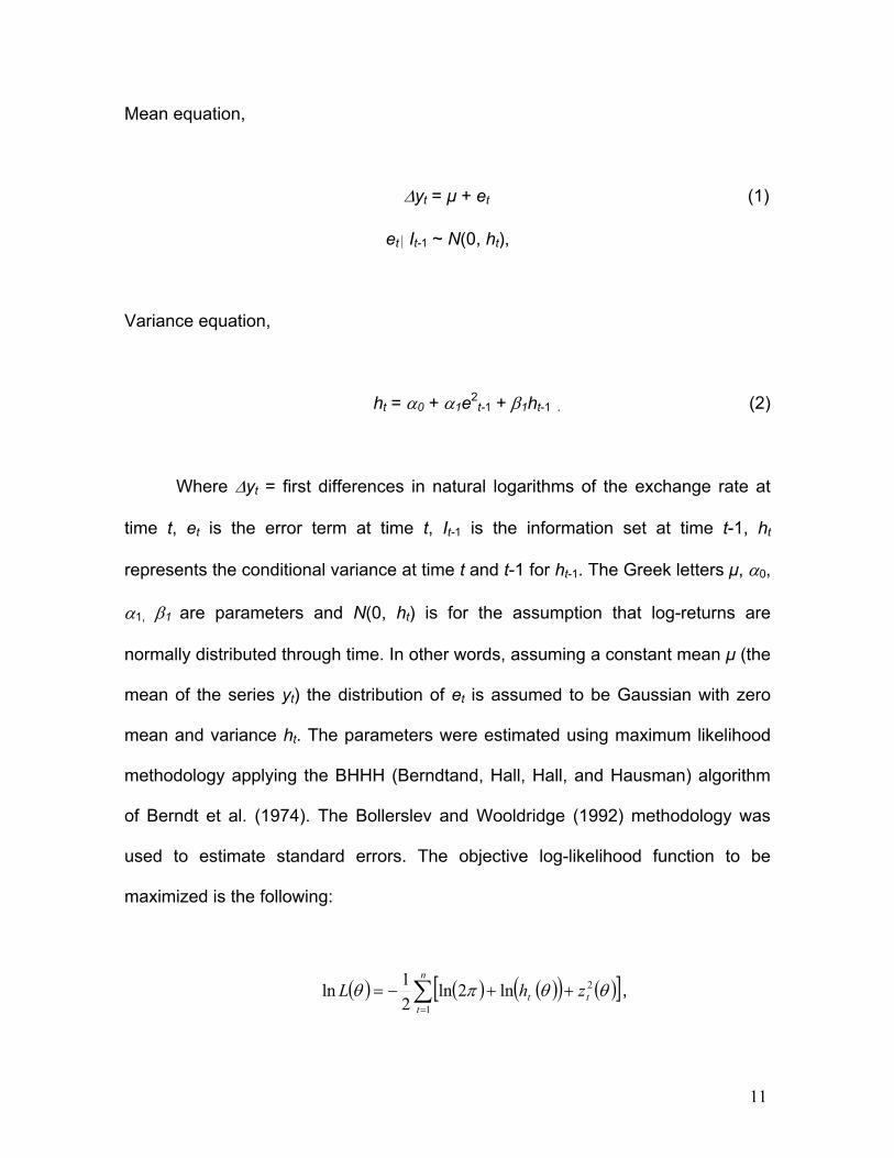
Mean equation,
∆yt = µ + et (1)
et It-1 ~ N(0, ht),
Variance equation,
ht = α0 + α1e2t-1 + β1ht-1 . (2)
Where ∆yt = first differences in natural logarithms of the exchange rate at
time t, et is the error term at time t, It-1 is the information set at time t-1, ht
represents the conditional variance at time t and t-1 for ht-1. The Greek letters µ, α0,
α1, β1 are parameters and N(0, ht) is for the assumption that log-returns are
normally distributed through time. In other words, assuming a constant mean µ (the
mean of the series yt) the distribution of et is assumed to be Gaussian with zero
mean and variance ht. The parameters were estimated using maximum likelihood
methodology applying the BHHH (Berndtand, Hall, Hall, and Hausman) algorithm
of Berndt et al. (1974). The Bollerslev and Wooldridge (1992) methodology was
used to estimate standard errors. The objective log-likelihood function to be
maximized is the following:
( ) ( ) ( )( ) ( )[ ]∑=
++−=n
ttt zhL
1
2ln2ln21ln θθπθ ,
12
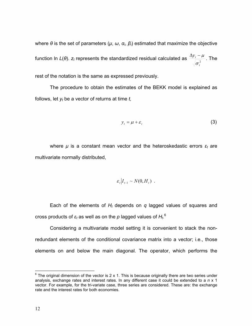
where θ is the set of parameters (µ, ω, αi, βi) estimated that maximize the objective
function ln L(θ). zt represents the standardized residual calculated as 2t
tyσ
µ−∆ . The
rest of the notation is the same as expressed previously.
The procedure to obtain the estimates of the BEKK model is explained as
follows, let yt be a vector of returns at time t,
tty εµ += (3)
where µ is a constant mean vector and the heteroskedastic errors εt are
multivariate normally distributed,
),0(~1 ttt HNI −ε .
Each of the elements of Ht depends on q lagged values of squares and
cross products of εt as well as on the p lagged values of Ht.6
Considering a multivariate model setting it is convenient to stack the non-
redundant elements of the conditional covariance matrix into a vector; i.e., those
elements on and below the main diagonal. The operator, which performs the
6 The original dimension of the vector is 2 x 1. This is because originally there are two series under analysis, exchange rates and interest rates. In any different case it could be extended to a n x 1 vector. For example, for the tri-variate case, three series are considered. These are: the exchange rate and the interest rates for both economies.
13
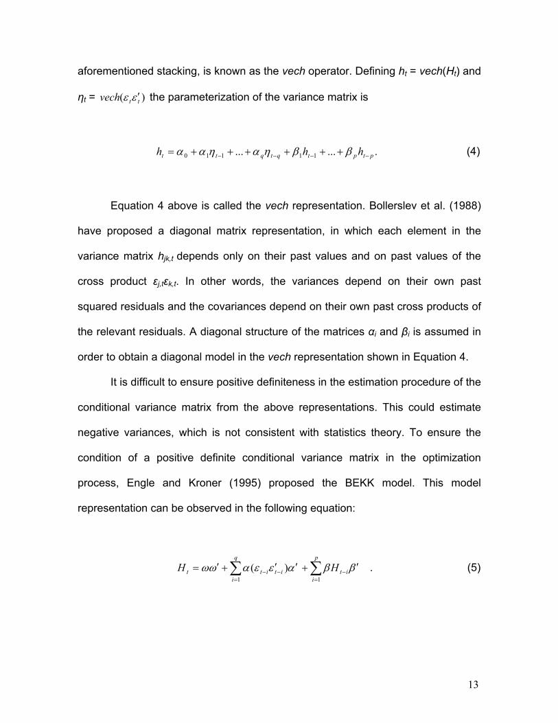
aforementioned stacking, is known as the vech operator. Defining ht = vech(Ht) and
ηt = )( ttvech εε ′ the parameterization of the variance matrix is
....... 11110 ptptqtqtt hhh −−−− ++++++= ββηαηαα (4)
Equation 4 above is called the vech representation. Bollerslev et al. (1988)
have proposed a diagonal matrix representation, in which each element in the
variance matrix hjk,t depends only on their past values and on past values of the
cross product εj,tεk,t. In other words, the variances depend on their own past
squared residuals and the covariances depend on their own past cross products of
the relevant residuals. A diagonal structure of the matrices αi and βi is assumed in
order to obtain a diagonal model in the vech representation shown in Equation 4.
It is difficult to ensure positive definiteness in the estimation procedure of the
conditional variance matrix from the above representations. This could estimate
negative variances, which is not consistent with statistics theory. To ensure the
condition of a positive definite conditional variance matrix in the optimization
process, Engle and Kroner (1995) proposed the BEKK model. This model
representation can be observed in the following equation:
ββαεεαωω ′+′′+′= −=
−−=
∑∑ it
p
iitit
q
it HH
11)( . (5)
14
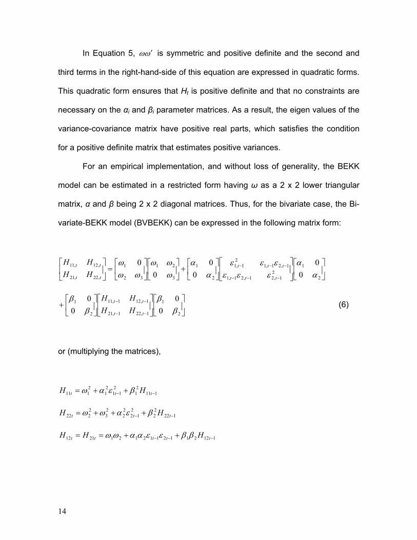
In Equation 5, ωω ′ is symmetric and positive definite and the second and
third terms in the right-hand-side of this equation are expressed in quadratic forms.
This quadratic form ensures that Ht is positive definite and that no constraints are
necessary on the αi and βi parameter matrices. As a result, the eigen values of the
variance-covariance matrix have positive real parts, which satisfies the condition
for a positive definite matrix that estimates positive variances.
For an empirical implementation, and without loss of generality, the BEKK
model can be estimated in a restricted form having ω as a 2 x 2 lower triangular
matrix, α and β being 2 x 2 diagonal matrices. Thus, for the bivariate case, the Bi-
variate-BEKK model (BVBEKK) can be expressed in the following matrix form:
+
=
−−−
−−−
2
12
1,21,21,1
1,21,12
1,1
2
1
3
21
32
1
,22,21
,12,11
00
00
00
αα
εεεεεε
αα
ωωω
ωωω
ttt
ttt
tt
tt
HHHH
+
−−
−−
2
1
1,221,21
1,121,11
2
1
00
00
ββ
ββ
tt
tt
HHHH
(6)
or (multiplying the matrices),
1112
12
1121
2111 −− ++= ttt HH βεαω
12222
212
22
23
2222 −− +++= ttt HH βεαωω
11221121121212112 −−− ++== ttttt HHH ββεεααωω
15
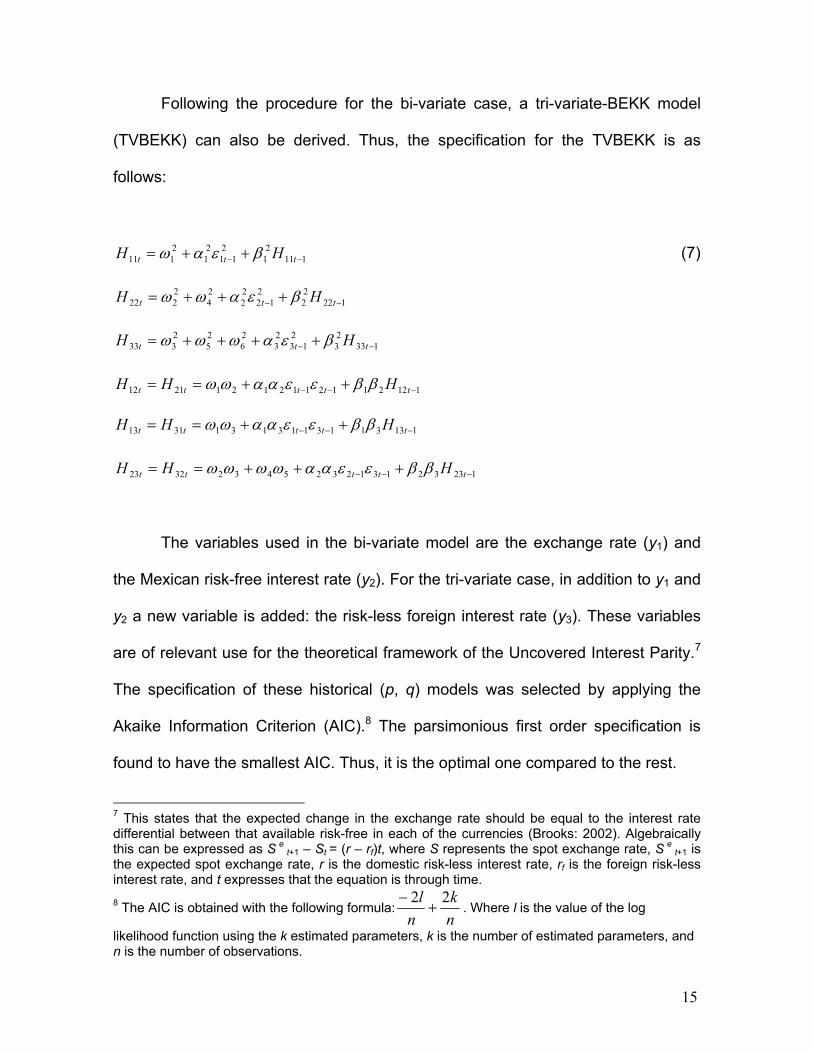
Following the procedure for the bi-variate case, a tri-variate-BEKK model
(TVBEKK) can also be derived. Thus, the specification for the TVBEKK is as
follows:
1112
12
1121
2111 −− ++= ttt HH βεαω (7)
122
22
212
22
24
2222 −− +++= ttt HH βεαωω
133
23
213
23
26
25
2333 −− ++++= ttt HH βεαωωω
11221121121212112 −−− ++== ttttt HHH ββεεααωω
11331131131313113 −−− ++== ttttt HHH ββεεααωω
1233213123254323223 −−− +++== ttttt HHH ββεεααωωωω
The variables used in the bi-variate model are the exchange rate (y1) and
the Mexican risk-free interest rate (y2). For the tri-variate case, in addition to y1 and
y2 a new variable is added: the risk-less foreign interest rate (y3). These variables
are of relevant use for the theoretical framework of the Uncovered Interest Parity.7
The specification of these historical (p, q) models was selected by applying the
Akaike Information Criterion (AIC).8 The parsimonious first order specification is
found to have the smallest AIC. Thus, it is the optimal one compared to the rest.
7 This states that the expected change in the exchange rate should be equal to the interest rate differential between that available risk-free in each of the currencies (Brooks: 2002). Algebraically this can be expressed as S e
t+1 – St = (r – rf)t, where S represents the spot exchange rate, S e t+1 is
the expected spot exchange rate, r is the domestic risk-less interest rate, rf is the foreign risk-less interest rate, and t expresses that the equation is through time. 8 The AIC is obtained with the following formula:
nk
nl 22+
−. Where l is the value of the log
likelihood function using the k estimated parameters, k is the number of estimated parameters, and n is the number of observations.
16
V.2. OPTION IMPLIED VOLATILITY
The option implied volatility of an underlying asset is the market’s forecast of
the volatility of such asset, obtained from the options written on the underlying
asset (Hull: 2003). To calculate the option implied volatility of an asset an option
valuation model together with inputs for that model are needed. The inputs for a
typical option valuation model are risk-free rate of interest, time to maturity, price of
the underlying asset, the exercise price, and the price of the option (Blair, Poon
and Taylor: 2001). Using an inappropriate valuation model will produce significantly
large pricing errors and option implied volatilities will be mis-measured (Harvey and
Whaley: 1992). For each trading day the aforementioned implied volatilities are
derived from at-the-money (ATM) over-the-counter (OTC) one month option
contracts for the Mexican peso - USD.
V.3. THE COMPOSITE FORECAST MODEL
In the spirit of Makridakis (1989), a composite forecast model is also
estimated. The composite forecast model includes estimates of the ARCH-type
models as well as estimates from implied volatilities. Considering that the time
variable in the option price formula is measured in years, estimates of the implied
volatilities are calculated on an annualized basis. In order to be consistent using
daily returns, the implied volatilities estimates in the composite forecast model
17
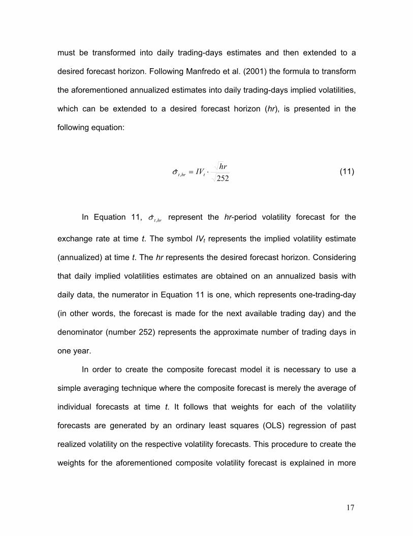
must be transformed into daily trading-days estimates and then extended to a
desired forecast horizon. Following Manfredo et al. (2001) the formula to transform
the aforementioned annualized estimates into daily trading-days implied volatilities,
which can be extended to a desired forecast horizon (hr), is presented in the
following equation:
252
ˆ ,rhIVthrt ⋅=σ (11)
In Equation 11, hrt ,σ represent the hr-period volatility forecast for the
exchange rate at time t. The symbol IVt represents the implied volatility estimate
(annualized) at time t. The hr represents the desired forecast horizon. Considering
that daily implied volatilities estimates are obtained on an annualized basis with
daily data, the numerator in Equation 11 is one, which represents one-trading-day
(in other words, the forecast is made for the next available trading day) and the
denominator (number 252) represents the approximate number of trading days in
one year.
In order to create the composite forecast model it is necessary to use a
simple averaging technique where the composite forecast is merely the average of
individual forecasts at time t. It follows that weights for each of the volatility
forecasts are generated by an ordinary least squares (OLS) regression of past
realized volatility on the respective volatility forecasts. This procedure to create the
weights for the aforementioned composite volatility forecast is explained in more
18
detail in Granger and Ramanathan (1984). This can be observed in the following
equation:
ttkkttt εσβσβσβασ +++++= ,,22,110 ˆ...ˆˆ . (12)
In Equation 12, tσ represent the realized volatility at time t, and tk ,σ
represent the individual volatility forecast (k) corresponding to the realized volatility
at period t. As it can be observed in this equation, the composite forecast model
includes the average of the individual volatility forecasts at time t. Following Blair,
Poon and Taylor (2001) the realized volatility can be calculated as follows:
∑=
+=hr
jjthrt R
1
2,
2σ , (13)
where σt,hr represents the realized (ex-post) volatility at time t over forecast
horizon hr. The R2t represents the squared log return at time period t. It is important
to point out that the volatility is not observed. The realized volatility represents a
‘proxy’ for the real volatility.9 However, this method is the most commonly used in
the volatility forecasting literature (Andersen and Bollerslev: 1998; Poon and
Granger: 2003; Andersen, et al. 2005). Thus, the resulting composite volatility
forecast can be observed in Equation 14 where the variables are the same as
expressed previously,
9 I am thankful to Daniel Chiquiar and Carlos Capistrán for asking me to clarify this.

19
1,1,221,1101 ˆˆ...ˆˆˆˆˆˆ ++++ ++++= tkkttt σβσβσβασ . (14)
The composite forecast model of this equation is a one-day volatility
forecast. In order to create a composite volatility forecast of more than one trading
day; i.e., hr > 1, the estimated one-day composite volatility forecast (from Equation
14) is multiplied by rh . The aforementioned method for obtaining a composite
volatility forecast of more than one day (h > 1) is a common practice in the
academic literature; however, it is important to emphasize that an alternative is to
obtain predictions of volatility for each period in the forecast interval (e.g. from an
ARCH model).
The MSE obtained from each of the estimates of all volatility forecast
models are compared with each other. The formula to obtain the MSE is presented
in Equation 15,
( )2
1,,1
2,, ˆ
1∑=
−−=n
iihrtihrtn
MSE σσ , (15)
where n is equal to the number of observations and the other variables are
the same as described previously. These MSE comparisons are performed in order
to provide a robust analysis of the accuracy of the aforementioned composite
volatility forecast model against the alternative models (the conditional and implied
volatilities models). The model with the smaller MSE is considered the most
accurate volatility forecasting model of the returns of the exchange rate. Ranking

20
models in terms of their MSE is a common practice in forecasting volatility literature
(Manfredo et al.: 2001). The procedure applied to obtain these statistical
significances is based on the method postulated by Diebold and Mariano (1995).10
VI. DATA
VI.1. OPTIONS AND SPOT DATA
The data for the spot exchange rate Mexican peso-USD consists of daily
spot prices obtained from Banco de México’s web page database.11 These are
daily averages of quotes offered by major Mexican banks and other financial
intermediaries. The option implied data is calculated from daily OTC options for 1-
month to maturity contracts of the Mexican peso-USD (the time to maturity of the
option contract is always fixed and equal to one month). The data was downloaded
from Bloomberg database. The ticker is USDMXNV1M.12 The data for the interest
rates consists of daily 30-day interest rates of Mexican Certificates of Deposit
(CDs) obtained from Banco de México’s web page. US CDs were obtained from
10 This method requires generating a time series, which is the differential of the squared-forecast
errors from two different forecast models; i.e.., ( ) ( )21,222
1,12 ˆˆ −− −−−= tttttd σσσσ , where dt is the
differential of the series and iσ is the forecast of the i model. The t-statistic is obtained in the
following way,:
nsdd
where d is the sample mean and sd is equal to the standard deviation of the
series (d). The notation for the other variables is the same as described previously. 11 Banco de México’s Web page is http://www.banxico.org.mx 12 Option implied volatility data obtained from a well-known international financial institution was also used. However, the results in the estimations show that the implied volatilities obtained from Bloomberg quotes were more accurate in terms of statistical tests. It was therefore decided to include only the latter for the present analysis. I am thankful to Alejandro Díaz de León for encouraging me to analyze additional series.
21
the Federal Reserve (FED) web page with the same maturity.13 The sample period
under analysis is more than five years, from 01/03/2000 to 01/09/2006. The sample
size consists of 1,295 daily observations.
VII. DESCRIPTIVE STATISTICS
This subsection presents the descriptive statistics for the ex post realized
volatilities of exchange rate returns and volatility forecasting models. Prior to fitting
the GARCH models, ARCH effects tests were conducted on the series under
analysis in order to corroborate if the series had ARCH effects, and therefore
assure that these types of models are appropriate for the data. The test conducted
was the ARCH-LM test following the procedure of Engle (1982). According to the
results, all the series under study; i.e., the spot and the interest rates, had ARCH
effects.14 Under the null of homoscedasticity in the errors, the F-statistics were
8.5119 for the spot, 12.9234 for the Mexican interest rates and 24.6407 for the US
interest rates. For all variables the null hypotheses were rejected in favor of
heteroscedasticity on those errors. Thus, the application of ARCH models is
statistically justified (the critical value is 6.63 at the limit for a 1% confidence level).
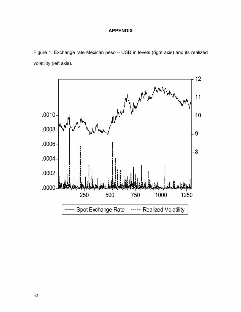
Figure 1 presents the spot exchange rate Mexican pesos per USD and its
realized volatility. Table 1 shows the descriptive statistics for the realized volatility
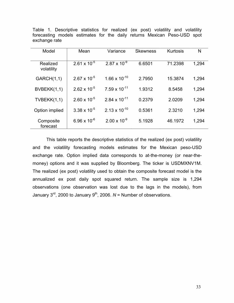
and the forecasting models. As it can be observed in Table 1, the means of the
13 The FED web page is http://www.federalreserve.gov/
14 These tests were conducted by regressing the logarithmic returns of the analyzed series under analysis against a constant. The ARCH-LM test is performed on the residuals of that regression. The test consists on regressing the square residuals against a constant and lagged values of the same square residuals. The statistical significance is tested with a F-Distribution. Five lags were applied in each test.
22
option implied volatilities are those with higher values. These findings are
consistent with Christensen and Prabhala (1998), who found that option implied
volatilities had higher first moments. The distributions of all variables are highly
skewed and leptokurtic, indicating the non-normality of the daily returns and the
forecast estimates. This is consistent with the work of Wei and Leuthold (1998),
who also corroborated the existence of non-normality in this type of data
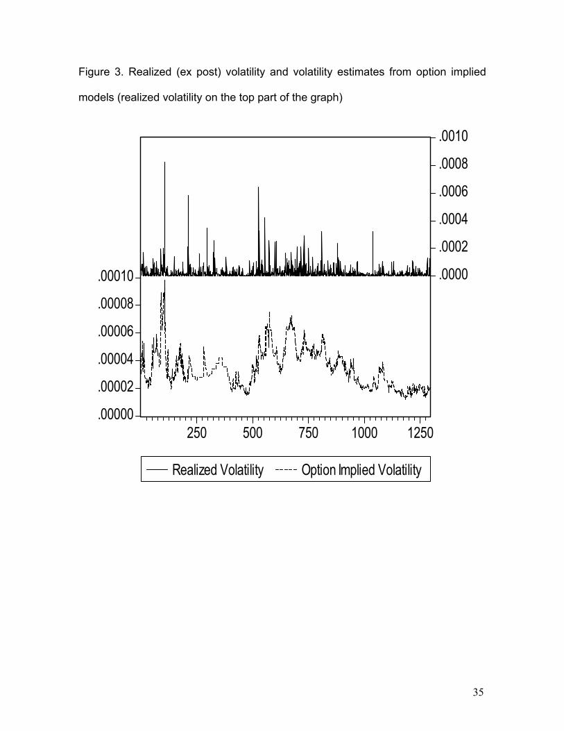
frequency. Last, Figures 2 and 3 presents the observations of the realized volatility
(top line) and estimates of the GARCH models and option implieds (bottom lines).
It can be observed that in both graphs all models capture the volatility clustering
periods shown with the realized volatility. At a simple sight, the implied volatility
models estimates are significantly greater than the realized volatility (Figure 3).
VIII. RESULTS
VIII.1. IN-SAMPLE EVALUATION
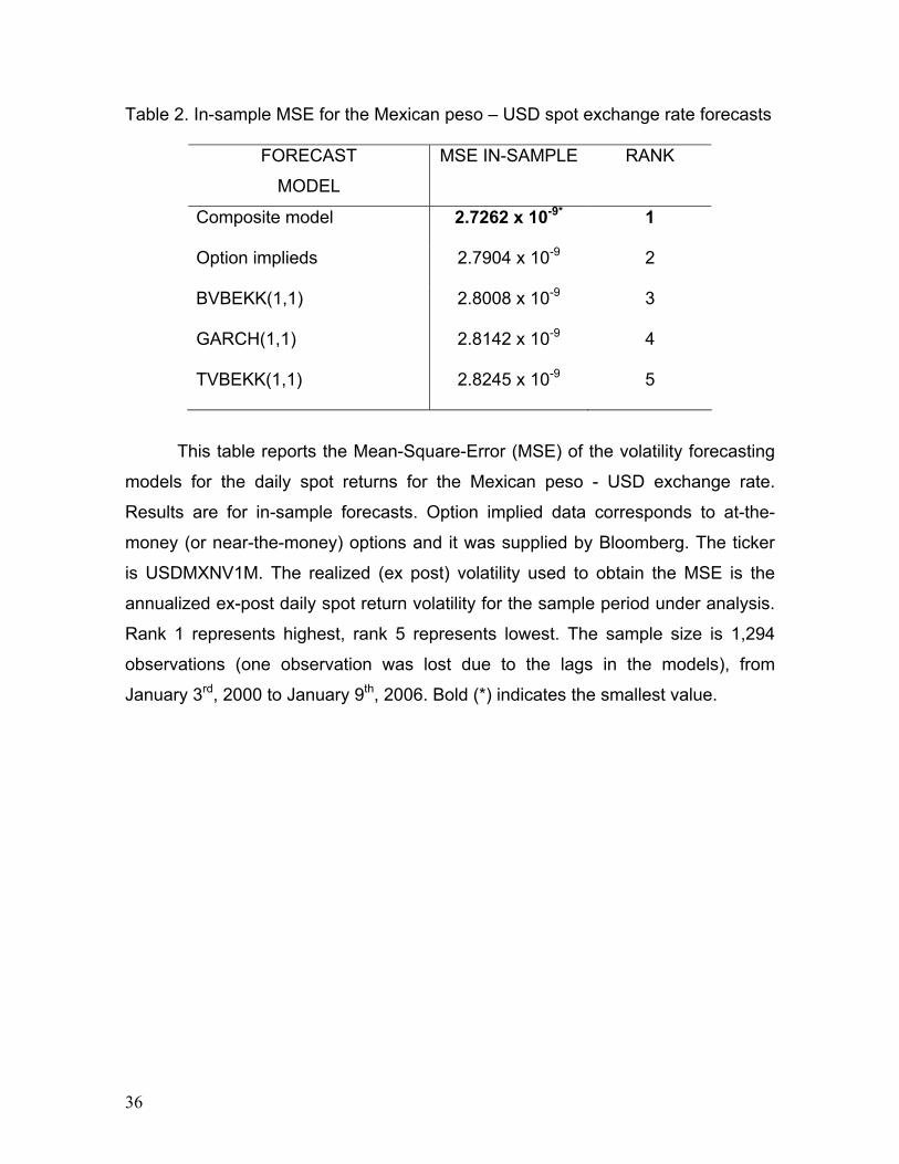
The MSE results are presented in Table 2. For the composite model the
BVBEKK and the option implied were chosen given that they had superior forecast
accuracy relative to their counterparts. The weights assigned to each model were
obtained from an OLS regression as explained in Section V.3. above. The option
implied volatilities had the higher weight, which was nearly 90%. On the other
hand, the BVBEKK model obtained only 10% of the weight. This shows that option
implied volatilities had higher information content compared with the multi-variate
GARCH model. From Table 2 it can be observed that the most accurate model is
23
the composite model given that it has the lowest MSE.15 The second best forecast
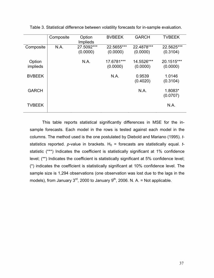
is the option implied volatility. When tests for statistical difference between the two
competing models were applied, the null hypothesis of equal forecasting accuracy
was rejected (see Table 3). This leads to the conclusion that there is forecast
superiority between the composite model and its counterparts. These results are
consistent with part of the literature that favors composite models in terms of better
forecasting accuracy. MSE differences among models (Table 3) are statistically
significant at 1%.
VIII.2. OUT-OF-SAMPLE EVALUATION
The sample period under analysis is partitioned in half in order to evaluate
the out-of-sample forecasts. Estimates (in-sample) for all models are obtained from
January 3rd, 2000 to January 22nd, 2003 for a total of 647 observations (about half
the total number of observations). The jump-off period is January 23rd, 2003. Thus,
the out-of-the-sample evaluation for all forecasting models is from January 23rd,
2003 to January 9th, 2006.
The forecast models chosen for the composite specification were those with
superior forecast accuracy (lowest MSE) in the in-sample evaluation. These were
the BVBEKK for the ARCH-type models and the option implieds. The weights
applied for the forecast estimates were qualitatively similar to those used in the in-
sample valuation i.e. around 90% for the option implied volatilities and around 10%
for the BVBEKK. The results of the MSE for each model including the composite
15 It is important to point out that several sample periods were tested for the composite model. These results were qualitatively similar to the ones presented in the present subsection. These results are available upon request.

24
specification are presented in Table 4. As observed in Table 4, in the out-of-the-
sample evaluation the composite model also has the lowest MSE. The second best
was option implied volatilities. The MSE statistical differences are presented in
Table 5. The results are qualitatively similar to those obtained for the in-sample
estimates. The forecasts were also estimated using rolling window and a recursive
approach. Since the results on both methods were qualitatively similar to the ones
explained above they are not reported.16
VIII.3. ANALYSIS OF THE RESULTS
The overall finding is that the composite model was superior in terms of
MSE. In statistical terms, the composite model’s estimated forecasts are
statistically different than its counterparts. Thus, the null hypothesis presented that
composite volatility forecasts models do not contain additional information content
of the realized (ex post) volatility is rejected. The predictive power of option
implieds has proven to be more accurate than the ARCH-type models. But if the
ARCH-type and option implied forecasts are combined in a composite approach,
the MSE becomes lower and statistically significant. This recommends the use of
both types of data when available. Finally, the results of this paper are in line with
those studies which favor composite specifications (Vasilellis and Meade: 1996;
Blair et. al.: 2001; Manfredo et. al.: 2001; Benavides: 2003, 2004). Also, that option
implied volatilities have more information content compared to ARCH-type models.
About 76% of similar types of studies have found that options implied volatilities
are more accurate in forecasting financial variables volatility compared with ARCH- 16 These results are available upon the reader’s request.
25
type models (Poon and Granger: 2003). The results of the present paper are
consistent with these studies.
IX. CONCLUSION
The on-going debate regarding which is the most accurate model to forecast
volatility of price returns of financial assets has led to a substantial amount of
research. Many have compared ARCH-type models against option implied
volatilities and composite forecast models. Albeit the majority of the literature
advocates the use of option implied volatilities as the most accurate alternative to
forecast price returns volatilities, no conclusion has been drawn in terms of finding
one superior model. This is because the statistical evaluation of the forecasts has
generally shown that the competing models have statistically equal accuracy.
In the present research paper the aforementioned volatility forecast models;
i.e., ARCH-type, option implieds and composite forecast models, were compared
with each other to find the most accurate volatility forecasting model for the daily
spot returns of the Mexican peso – US Dollar exchange rate. Tests were performed
for both in-sample and out-of-sample evaluations. Rolling windows and recursive
methods were also applied. Even though option implied volatilities contained most
of the information content of the realized spot return volatility, the composite
forecast was superior one. The weights in the composite specification were
obtained with a OLS regression. These were about 90% for option implied
volatilities and about 10% for the bi-variate BEKK model. In addition, there was
statistical significant difference between ARCH-type models, option implieds and
composite approach forecasts. The null hypothesis of no additional information
26
content for composite models is, therefore, rejected. Considering the evaluation of
forecast estimates in terms of their statistical differences, it is concluded that the
composite model is the most accurate. Finally, a word of caution is given to these
conclusions given that not all assumptions were met when estimating the models.
Specially, the normality assumption for the ARCH-type models is highly
questioned.
27
BIBLIOGRAPHY
Andersen, T, G., Bollerslev, T., Christoffersen, P. F., and Diebold, F.X. (2005). Volatility and Correlation Forecasting. Handbook of Economic Forecasting. Edited by G. Elliot., C.W.J. Granger., and A. Timmermann. Amsterdam: North Holland. Andersen, T, G., and Bollerslev, T. (1998). Answering the Skeptics: Yes, Standard Volatility Models Do Provide Accurate Forecasts. International Economic Review. Vol. 39 (885-905). Akgiray, V. (1989). Conditional Heteroscedasticity in Time Series of Stock Returns: Evidence and Forecasts. Journal of Business. Vol. 62. (55-80). Baba, Y., Engle, R. F., Kroner, K. F. and Kraft, D. (1992). Multivariate Simultaneous Generalized ARCH. Economics Working Paper 92 – 5. University of Arizona, Tucson. Barone-Adesi, G. and Whaley, R. E. (1987). Efficient Approximation of American Option Values. The Journal of Finance. Vol. 42. June. (301-320). Bates, J. M. and Granger, C. W. J. (1969). The Combination of Forecasts. Operations Research Quarterly. Vol. 20. (451 – 468). Benavides, G. (2003). Price Volatility Forecasts for Agricultural Commodities: An Application of Historical Volatility Models, Option Implieds and Composite Approaches for Futures Prices of Corn and Wheat. Working paper. Benavides, G. (2004). Predictive Accuracy of Futures Option Implied Volatility: The Case of the Exchange Rate Futures Mexican Peso - US Dollar. Working paper. Berndtand, E. Hall, B. Hall, R. and Hausman, J. (1974). Estimation and Inference in Nonlinear Structural Models. Annals of Economic and Social Measurement. (653-665). Bessler, D. A. and Brandy, J. A. (1981). Forecasting Livestock Prices with Individual and Composite Methods. Applied Economics. Vol. 13. (513 – 522).
28
Black, F. and Scholes, M. S. (1973). The Pricing of Options and Corporate Liabilities. Journal of Political Economy. Vol. 81. May-June (637 – 654). Blair, B. J., Poon, S. and Taylor, S. J. (2001). Forecasting S&P 100 Volatility: The Incremental Information Content of Implied Volatilities and High-Frequency Index Returns. Journal of Econometrics. Vol. 105. (5-26). Bollerslev, T. P. (1986). Generalized Autoregressive Conditional Heteroscedasticity. Journal of Econometrics. Vol. 31. (307-327). Bollerslev, T., Engle, R. and Wooldridge, J. (1988) A Capital Asset Pricing Model with Time-Varying Covariances. Journal of Political Economy. No. 96. (116-131). Bollerslev, T. P., Chou, R. Y. and Kroner, K. F. (1992). ARCH Modeling in Finance: A Review of the Theory and Empirical Evidence. Journal of Econometrics 52 (5-59). Brooks, C., Henry, O. T. and Persand, G. (2002). Optimal Hedging and the Value of the News. Journal of Business. Vol. 75. Issue 2. (333-52). Brooks, C. (2002). Introductory Econometrics for Finance. Cambridge University Press. Christensen, B. J., and Prabhala, N. R. (1998). The Relation between Implied and Realized Volatility. Journal of Financial Economics. Volume 50, Issue 2, November: (125-150). Chu, S. H. and Freund, S. (1996). Volatility Estimation for Stock Index Options: A GARCH Approach. Quarterly Review of Economics and Finance. Vol. 36. (431-450). Clemen, R. T. (1989). Combining Forecasts: A Review and Annotated Bibliography. International Journal of Forecasting. Vol. 5. (559 – 583). Clements, M. P. and Hendry, D. F. (1998). Forecasting Economic Time Series. Cambridge: Cambridge University Press. Day, T. E. and Lewis, C. M. (1992). Stock Market Volatility and the Information Content of Stock Index Options. Journal of Econometrics. Vol. 52. (267-287).
29
Diebold, F. X. and Mariano, R. S. (1995). Comparing Predictive Accuracy. Journal of Business and Economic Statistics. Vol. 13. (253-263). Ederington, L. and Guan, W. (2002). Is implied Volatility an Informationally Efficient and Effective Predictor of Future Volatility? Journal of Risk. Vol. 4 (3). Engle, R. F. (1982) “Autoregressive Conditional Heteroskedasticity with Estimates of the Variance of U.K. Inflation,” Econometrica, 50, (987–1008). Engle, R. F. (2000). Dynamic Conditional Correlation – A Simple Class of Multivariate GARCH Models. SSRN Discussion Paper 2000-09. University of California, San Diego. May 2000. Engle, R. F. and Kroner, K. (1995). Multivariate Simultaneous Generalized ARCH. Econometric Theory 11. (122-150). Fang, Y. (2002). Forecasting Combination and Encompassing Tests. International Journal of Forecasting. Vol. 1. Elsevier Science B. V. Figlewski, S. (1997). Forecasting Volatility. Financial Markets, Institutions, and Instruments. Vol. 6. (2-87). Fleming, J. (1998). The Quality of Market Volatility Forecasts Implied by S & P 100 Index Option Prices. Journal of Empirical Finance. Vol. 5. (317-345). Garman, M.B. and Kohlhagen, S. W. (1983). Foreign Currency Option Values. Journal of International Money and Finance. Vol. 2. pp. 231-37, May. Giot, P. (2003). Implied Volatility Indexes and Daily Value-at-Risk Models. Working paper. Department of Business Administration & CEREFIM at University of Namur, Belgium. Granger, C. W. J. and Ramanathan, R. (1984). Improved Methods of Combining Forecasts. Journal of Forecasting. Vol. 3. (197-204). Granger, C. W. J. (2001). Long Memory Process-An Economist’s Viewpoint. Working paper University of California at San Diego. Harvey, C. R. and Whaley, R. E. (1992). Dividends and S&P 100 Index Options. Journal of Futures Markets. Vol. 12. (123 – 137). Hull, J. (2003). Options, Futures and Other Derivatives. 5th. Edition. Prentice Hall.
30
Jorion, P. (1995). Predicting Volatility in the Foreign Exchange Market. The Journal of Finance. Vol. 50 (507-528). Kroner, K., Kneafsey, K. P. and Claessens, S. (1994). Forecasting Volatility in Commodity Markets. Journal of Forecasting. Vol. 14. (77-95). Lamoureux, C. G. and Lastrapes, W. D. (1993). Forecasting Stock Return Variance: Toward an Understanding of Stochastic Implied Volatilities. The Review of Financial Studies. Vol. 6. (293-326). Levich R. M. (1998). International Financial Markets: Prices and Policies. Boston, Mass.: Irwin McGraw-Hill. Makridakis, S. (1989). Why Combining Works? International Journal of Forecasting. Vol. 5. (601-603). Manfredo, M. Leuthold, R. M. and Irwin, S. H. (2001). Forecasting Cash Price Volatility of Fed Cattle, Feeder Cattle and Corn: Time Series, Implied Volatility and Composite Approaches. Journal of Agricultural and Applied Economics. Vol. 33. Issue 3. December. (523-538). Markowitz, H. (1952). Portfolio Selection. The Journal of Finance. Vol. VII, No. 1. March. Martens, M., and Zein, J. (2002). Predicting Financial Volatility: High-Frequency Time-Series Forecasts vis-à-vis Implied Volatility, Mimeo, Erasmus University Rotterdam. Neely, C.J., (2002). Forecasting Foreign Exchange Volatility: Is implied Volatility the Best We Can Do? Federal Reserve Bank of St. Louis, Working paper 2002-017. Ng, V. K and Pirrong, S. C. (1994). Fundamentals and Volatility: Storage, Spreads, and the Dynamic of Metals Prices. Journal of Business 67 (203-230). Park, D. W. and Tomek, W. G. (1989). An Appraisal of Composite Forecasting Methods. North Central Journal of Agricultural Economics. Vol. 10. (1-11). Poon, S-H. and Granger, C. (2003). Forecasting Volatility in Financial Markets: A Review, Journal of Economic Literature. Vol. 41. No. 2, June. (478-539). Pong, S., Shackleton, M., Taylor, S. and Xu, X. (2003). Forecasting Currency Volatility: A Comparison of Implied Volatilities and AR(FI)MA models. Forthcoming, Journal of Banking and Finance.
31
Schroeder, T. C., Albright, M. L., Langemeier, M. R. and Mintert, J. (1993). Factors Affecting Cattle Feeding Profitability. Journal of the American Society of Farm Managers and Rural Appraisers. 57: (48-54). Susmel, R. and Thompson, R. (1997). Volatility, Storage and Convenience Evidence from Natural Gas Markets. Journal of Futures Markets. Vol. 17. No. 1 (17-43). Taylor, S. J. (1985). The Behavior of Futures Prices Overtime. Applied Economics, 17:4 Aug: (713-734). Taylor, S. J. (1986). Modeling Financial Time Series. Wiley. Vasilellis, G. A. and Meade, N. (1996). Forecasting Volatility for Portfolio Selection. Journal of Business Finance and Accounting. Vol. 23 (125-143). Wei, A. and Leuthold, R. M. (1998). Long Agricultural Futures Prices: ARCH, Long Memory, or Chaos Processes. OFOR Paper Number 98-03. Xu, X. and Taylor, S. J. (1995). Conditional Volatility and the Informational Efficiency of the PHLX Currency Options Market. Journal of Banking and Finance. Vol. 19, (803-821).
32
APPENDIX
Figure 1. Exchange rate Mexican peso – USD in levels (right axis) and its realized
volatility (left axis).
.0000
.0002
.0004
.0006
.0008
.0010
8
9
10
11
12
250 500 750 1000 1250
Spot Exchange Rate Realized Volatility
33
Table 1. Descriptive statistics for realized (ex post) volatility and volatility forecasting models estimates for the daily returns Mexican Peso-USD spot exchange rate
Model Mean Variance Skewness Kurtosis N
Realized volatility
2.61 x 10⁻⁵ 2.87 x 10⁻⁹ 6.6501 71.2398 1,294
GARCH(1,1) 2.67 x 10⁻⁵ 1.66 x 10⁻¹⁰ 2.7950 15.3874 1,294
BVBEKK(1,1)
2.62 x 10⁻⁵ 7.59 x 10⁻¹¹ 1.9312 8.5458 1,294
TVBEKK(1,1)
2.60 x 10⁻⁵ 2.84 x 10⁻¹¹ 0.2379 2.0209 1,294
Option implied
3.38 x 10⁻⁵ 2.13 x 10⁻¹⁰ 0.5361 2.3210 1,294
Composite forecast
6.96 x 10⁻⁶ 2.00 x 10⁻⁹ 5.1928 46.1972 1,294
This table reports the descriptive statistics of the realized (ex post) volatility
and the volatility forecasting models estimates for the Mexican peso-USD
exchange rate. Option implied data corresponds to at-the-money (or near-the-
money) options and it was supplied by Bloomberg. The ticker is USDMXNV1M.
The realized (ex post) volatility used to obtain the composite forecast model is the
annualized ex post daily spot squared return. The sample size is 1,294
observations (one observation was lost due to the lags in the models), from
January 3rd, 2000 to January 9th, 2006. N = Number of observations.

34
Figure 2. Realized (ex post) volatility and volatility estimates from ARCH-type
models (realized volatility on the top part of the graph).
.00000
.00004
.00008
.00012
.00016.0000
.0002
.0004
.0006
.0008
.0010
250 500 750 1000 1250
Realized VolatilityGARCH(1,1)BVBEKK(1,1)
35
Figure 3. Realized (ex post) volatility and volatility estimates from option implied
models (realized volatility on the top part of the graph)
.00000
.00002
.00004
.00006
.00008
.00010 .0000
.0002
.0004
.0006
.0008
.0010
250 500 750 1000 1250
Realized Volatility Option Implied Volatility
36
Table 2. In-sample MSE for the Mexican peso – USD spot exchange rate forecasts
FORECAST
MODEL
MSE IN-SAMPLE RANK
Composite model 2.7262 x 10-9* 1
Option implieds 2.7904 x 10⁻⁹ 2
BVBEKK(1,1) 2.8008 x 10⁻⁹ 3
GARCH(1,1) 2.8142 x 10⁻⁹ 4
TVBEKK(1,1) 2.8245 x 10⁻⁹ 5
This table reports the Mean-Square-Error (MSE) of the volatility forecasting
models for the daily spot returns for the Mexican peso - USD exchange rate.
Results are for in-sample forecasts. Option implied data corresponds to at-the-
money (or near-the-money) options and it was supplied by Bloomberg. The ticker
is USDMXNV1M. The realized (ex post) volatility used to obtain the MSE is the
annualized ex-post daily spot return volatility for the sample period under analysis.
Rank 1 represents highest, rank 5 represents lowest. The sample size is 1,294
observations (one observation was lost due to the lags in the models), from
January 3rd, 2000 to January 9th, 2006. Bold (*) indicates the smallest value.
37
Table 3. Statistical difference between volatility forecasts for in-sample evaluation.
Composite Option Implieds
BVBEEK GARCH TVBEEK
Composite N.A. 27.5092*** (0.0000)
22.5655*** (0.0000)
22.4878*** (0.0000)
22.5625*** (0.3104)
Option implieds
N.A. 17.6781*** (0.0000)
14.5526*** (0.0000)
20.1515*** (0.0000)
BVBEEK N.A. 0.9539 (0.4020)
1.0146 (0.3104)
GARCH N.A. 1.8083*
(0.0707)
TVBEEK N.A.
This table reports statistical significantly differences in MSE for the in-
sample forecasts. Each model in the rows is tested against each model in the
columns. The method used is the one postulated by Diebold and Mariano (1995). t-
statistics reported. p-value in brackets. H0 = forecasts are statistically equal. t-
statistic (***) Indicates the coefficient is statistically significant at 1% confidence
level; (**) Indicates the coefficient is statistically significant at 5% confidence level;
(*) indicates the coefficient is statistically significant at 10% confidence level. The
sample size is 1,294 observations (one observation was lost due to the lags in the
models), from January 3rd, 2000 to January 9th, 2006. N. A. = Not applicable.
38
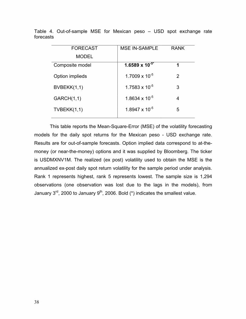
Table 4. Out-of-sample MSE for Mexican peso – USD spot exchange rate forecasts
FORECAST
MODEL
MSE IN-SAMPLE RANK
Composite model 1.6589 x 10-5* 1
Option implieds 1.7009 x 10⁻⁵ 2
BVBEKK(1,1) 1.7583 x 10⁻⁵ 3
GARCH(1,1) 1.8634 x 10⁻⁵ 4
TVBEKK(1,1) 1.8947 x 10⁻⁵ 5
This table reports the Mean-Square-Error (MSE) of the volatility forecasting
models for the daily spot returns for the Mexican peso - USD exchange rate.
Results are for out-of-sample forecasts. Option implied data correspond to at-the-
money (or near-the-money) options and it was supplied by Bloomberg. The ticker
is USDMXNV1M. The realized (ex post) volatility used to obtain the MSE is the
annualized ex-post daily spot return volatility for the sample period under analysis.
Rank 1 represents highest, rank 5 represents lowest. The sample size is 1,294
observations (one observation was lost due to the lags in the models), from
January 3rd, 2000 to January 9th, 2006. Bold (*) indicates the smallest value.

39
TABLE 5. Statistical difference between volatility forecasts for the out-of-sample evaluation.
Composite Option Implieds
BVBEEK GARCH TVBEEK
Composite N.A. 19.1532*** (0.0000)
11.3182*** (0.0000)
9.2582*** (0.0000)
9.3675*** (0.3104)
Option implieds
N.A. 9.7268*** (0.0000)
5.2489*** (0.0000)
10.0258*** (0.0000)
BVBEEK N.A. 0.0011 (0.9991)
0.0008 (0.994)
GARCH N.A. 0.0002
(0.9998)
TVBEEK N.A.
This table reports statistical significantly differences in MSE for out-of-
sample forecasts. Each model in the rows is tested against each model in the
columns. The method used is the one postulated by Diebold and Mariano (1995). t-
statistics reported. p-value in brackets. H0 = forecasts are statistically equal. t-
statistic (***) Indicates the coefficient is statistically significant at 1% confidence
level; (**) Indicates the coefficient is statistically significant at 5% confidence level;
(*) indicates the coefficient is statistically significant at 10% confidence level. The
sample size is 1,294 observations (one observation was lost due to the lags in the
models), from January 3rd, 2000 to January 9th, 2006. N. A. = Not applicable.