Analytical and experimental investigation The Author(s ...people.cst.cmich.edu/barry1o/assets/pdf/Analytical_and... · Article Analytical and experimental investigation of overhead

Article

Analytical and experimental investigationof overhead transmission line vibration

O Barry1, JW Zu1 and DCD Oguamanam2

Abstract

The vibration of a single-conductor transmission line with a Stockbridge damper is examined by modeling the system as a

double-beam concept. The equations of motion are derived using Hamilton’s principle, and expressions are presented for

the frequency equation, mode shapes, and orthogonality conditions. The analytical results are validated experimentally.

The effect of the damper characteristics and location on the system natural frequencies is investigated via a parametric

study. The role of the latter with respect to frequency is inconclusive. The present approach enables transmission lines

designers to determine the exact natural frequencies and mode shapes that are required in the study of the vibrational

response of a single conductor with a Stockbridge damper.

Keywords

Stockbridge damper, Strouhal frequency, messenger

1. Introduction

The vibration of overhead transmission lines is one ofthe most crucial factors that contribute to power out-ages. This is a wind-induced high-frequency low-amplitude vibration. The frequency of vibration variesbetween 3 and 150Hz and causes a peak-to-peak amp-litude of up to one conductor diameter. Stockbridgedampers are often employed to eliminate or reducethis vibration. Their effectiveness is highly dependenton their overall characteristic, location, and the char-acteristic of the conductor.

Several authors have studied the vibration of trans-mission lines. The most common approach is a com-bination of a numerical and an experimental method(Claren and Diana, 1969; Dhotard et al., 1978; Nigoland Houston, 1985; Kraus and Hagedorn, 1991;Vecchiarelly et al., 2000; Verma and Hagerdorn, 2004;Chan and Lu, 2007). The single conductor is usuallymodeled as an axially loaded Euler–Bernoulli beamwhile the Stockbridge damper is represented by asingle concentrated force on the conductor. The forceis expressed in terms of the velocity of the conductor atthe point of attachment of the damper and damperimpedance, which are usually obtained experimentally.

An attempt to depart from the above-mentionedconventional methods of modeling a single-conductortransmission line was reported by Barry et al.

(2011, 2013). Both conductor and damper were mod-eled as one unified system in order to account for theirtwo-way coupling. The finite element method was usedto determine the system natural frequencies and timeresponses. While the efficacy of the finite element modelwas demonstrated, the procedure was very complicatedand computationally intensive. Further, the finite elem-ent method is an approximate technique. The aim ofthe present study was to address these shortcomingsby presenting an analytical approach that yieldedexact solutions (in that the equations of motion andboundary conditions are satisfied exactly) with minimalcomplications.

The proposed model was based on double-beamconcepts. The conductor was modeled as an axiallyloaded Euler–Bernoulli beam and the Stockbridgedamper was modeled as an Euler–Bernoulli beamwith rigid tip masses. The Stockbridge damper was

1Department of Mechanical and Industrial Engineering, The University of

Toronto, Canada2Department of Mechanical and Industrial Engineering, Ryerson

University, Toronto, Canada

Corresponding author:

O Barry, Department of Mechanical and Industrial Engineering,

The University of Toronto, Toronto, Ontario M5S 3G8, Canada.

Email: [email protected]

Received: 27 July 2013; accepted: 6 November 2013

Journal of Vibration and Control

2015, Vol. 21(14) 2825–2837

! The Author(s) 2014

Reprints and permissions:

sagepub.co.uk/journalsPermissions.nav

DOI: 10.1177/1077546313517589

jvc.sagepub.com

at CMU Libraries - library.cmich.edu on May 16, 2016jvc.sagepub.comDownloaded from

http://jvc.sagepub.com/

arbitrarily located along the span of the conductor.Numerous studies on the vibration of double-beam/string systems abound in the literature (Yamaguchi,1984; Oguamanam et al., 1998; Oniszczuk, 2000; Vuet al., 2000; Oniszczuk, 2003; Abu-Hilal, 2006; Foda,2009; Palmeri and Adhikari, 2011; Foda, 2013).However, these investigations were either limited tocases where both beams were continuously connectedby viscous elastic layers or where one of the beams wasattached to the tip of the other.

In spite of this interest, there are no investigationswhere the primary beam is axially loaded and/or sup-porting in-span beam with tip mass. The use of thisconcept to analytically model a single-conductor trans-mission line with a Stockbridge damper was examinedin this study for the first time. The equations of motionwere derived using Hamilton’s principle. The expres-sions for the characteristic equation, mode shapes,and orthogonality relations are presented. The analyt-ical results were experimentally validated. Parametricstudies were then used to examine the effect of thedamper characteristics and location on the system nat-ural frequencies.

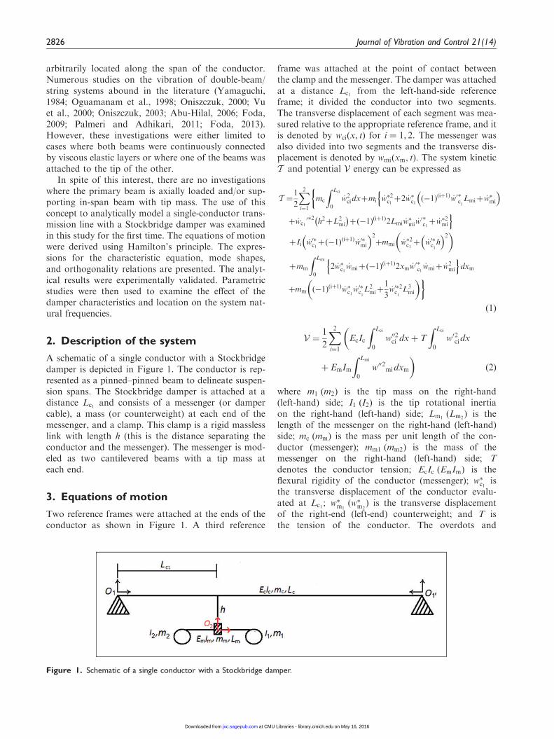
2. Description of the system

A schematic of a single conductor with a Stockbridgedamper is depicted in Figure 1. The conductor is rep-resented as a pinned–pinned beam to delineate suspen-sion spans. The Stockbridge damper is attached at adistance Lc1 and consists of a messenger (or dampercable), a mass (or counterweight) at each end of themessenger, and a clamp. This clamp is a rigid masslesslink with length h (this is the distance separating theconductor and the messenger). The messenger is mod-eled as two cantilevered beams with a tip mass ateach end.

3. Equations of motion

Two reference frames were attached at the ends of theconductor as shown in Figure 1. A third reference

frame was attached at the point of contact betweenthe clamp and the messenger. The damper was attachedat a distance Lc1 from the left-hand-side referenceframe; it divided the conductor into two segments.The transverse displacement of each segment was mea-sured relative to the appropriate reference frame, and itis denoted by wciðx, tÞ for i ¼ 1, 2. The messenger wasalso divided into two segments and the transverse dis-placement is denoted by wmiðxm, tÞ. The system kineticT and potential V energy can be expressed as

T ¼1

2

X2i¼1

mc

Z Lci

0

_w2cidxþmi _w�2c1 þ2 _w�c1 ð�1Þ

ðiþ1Þ _w0�

c1Lmiþ _w�mi

� �n�

þ _wc10�2 h2þL2

mi

� �þð�1Þðiþ1Þ2Lmi _w�mi _w0

�

c1þ _w�2mi

oþIi _w0�c1þð�1Þ

ðiþ1Þ _w0�mi

� �2þmmi _w�2c1 þ _w0�c

1h

� �2� �

þmm

Z Lmi

0

2 _w�c1 _wmiþð�1Þðiþ1Þ2xm _w0

�

c1_wmiþ _w2

mi

n odxm

þmm ð�1Þðiþ1Þ _w�c1 _w0�c

1L2miþ

1

3_w0�2c

1L3mi

� �ð1Þ

V ¼1

2

X2i¼1

EcIc

Z Lci

0

w002ci dxþ T

Z Lci

0

w02cidx

�

þ EmIm

Z Lmi

0

w002midxm

�ð2Þ

where m1 ðm2Þ is the tip mass on the right-hand(left-hand) side; I1 ðI2Þ is the tip rotational inertiaon the right-hand (left-hand) side; Lm1

ðLm2Þ is the

length of the messenger on the right-hand (left-hand)side; mc ðmmÞ is the mass per unit length of the con-ductor (messenger); mm1 ðmm2Þ is the mass of themessenger on the right-hand (left-hand) side; Tdenotes the conductor tension; EcIc ðEmImÞ is theflexural rigidity of the conductor (messenger); w�c1 isthe transverse displacement of the conductor evalu-ated at Lc1; w�m1

ðw�m2Þ is the transverse displacement

of the right-end (left-end) counterweight; and T isthe tension of the conductor. The overdots and

Figure 1. Schematic of a single conductor with a Stockbridge damper.

2826 Journal of Vibration and Control 21(14)



primes denote temporal and spatial derivation,respectively.

The equations of motion, equations (3) and (4), wereobtained by substituting the energy expressions inHamilton’s principle and taking the variations of thefield variables (�wc1 , �wc2 , �wm1

, and �wm2),

mc €wci þ EcIcw0000

ci � Tw00ci ¼ 0 ð3Þ

mm €w�c1 þ ð�1Þðiþ1Þ €w

0�c1Lmi þ €wmi

� �þ EmImw

0000mi ¼ 0

ð4Þ

Note that the subscript ‘i’ 2 ½1, 2� identifies the right-hand and left-hand segments of both the conductor andmessenger. The continuity conditions of the displace-ment at the attachment point of the damper to theconductor, Lc1 , yielded the following equations:

wc1 Lc1 , t� �

¼ wc2 Lc2 , t� �

ð5Þ

w0c1 Lc1 , t� �

¼ �w0c2 Lc2 , t� �

ð6Þ

From the variation of the conductor displacement,�wc1 , the obtained shear force boundary condition atthe location of the damper may be written as

X2i¼1

mi €w�c1 þ ð�1Þðiþ1Þ €w0�c

1Lmi þ €w�mi

� �þ €w�c1mmi

n

þmm

Z Lmi

0

€wmidxm þ1

2mm €w0

�

c1ð�1Þðiþ1ÞL2

mi

� EcIc w000�c1 þ w000�c2

� �þ T w0�c1

þw0�c2 Þ ¼ 0ð7Þ�

The contributions from the tension vanished because ofequation (6). The bending moment boundary conditionat the attachment of the messenger may be expressed as

X2i¼1

(mi ð�1Þ

ðiþ1Þ €w�c1Lmiþwc0� h2þL2

mi

� �þð�1Þðiþ1ÞLmi €w�mi

h i

þIi €w0�c1þð�1Þðiþ1Þ €w0�mi

� �þ €w0�c1h

2mmi

þmm

Z Lmi

0

ð�1Þðiþ1Þxm €wmidxm

þ1

2mm ð�1Þ

ðiþ1Þ €w�c1L2miþ

2

3€w0�c

1L3mi

� �)

þEcIc w00�c1 �w00�c2

� �¼0 ð8Þ

The last set of boundary conditions for the conductorwas obtained by enforcing no displacement and bend-ing moment at both ends of each segment:

wcið0, tÞ ¼ 0 ð9Þ

w00cið0, tÞ ¼ 0 ð10Þ

With respect to the messenger, the shear force bound-ary conditions at each end, Lm1

and Lm2, can be

expressed as

mi €w�mi þ €w�c1 þ ð�1Þðiþ1ÞLmi €w0�c1

� �� EmImw

000�mi ¼ 0 ð11Þ

and the bending moment boundary condition at eachend is

Ii €w0�

mi þ ð�1Þðiþ1Þ €w0

�

c1

� �þ EmImw

00�

mi ¼ 0 ð12Þ

The Stockbridge damper behaves as a cantileveredbeam at the junction of the clamp and the messengerxm ¼ 0. Hence, the displacement and rotation of boththe right- and left-side messengers are zero:

wmið0, tÞ ¼ 0 ð13Þ

w0mið0, tÞ ¼ 0 ð14Þ

4. Frequency equation andmode shapes

The transverse vibration displacement for each segmentof the conductor and messenger can be expressed as

wciðx, tÞ ¼ YciðxÞei!t ð15Þ

wmiðxm, tÞ ¼ YmiðxÞei!t ð16Þ

Substituting the above equations (equations (15) and(16)) into the equations of motion (equations (3)and (4)) yielded

Y00ci00 � S2Y00ci ��4

cYci ¼ 0 ð17Þ

Y000mi ��4mYmi ¼ �4

m Y�c1 þ ð�1Þðiþ1ÞY0�c1xm

� �ð18Þ

where

�c ¼!2mc

EcIc

� �14

�m ¼!2mm

EmIm

� �14

and

S ¼

ffiffiffiffiffiffiffiffiffiT

EcIc

r

Barry et al. 2827



The solutions of the above differential equations can beexpressed as

YciðxÞ ¼ A1i sin�xþ A2i cos�xþ A3i sinh �x

þ A4i cosh�x ð19Þ

YmiðxmÞ ¼ B1i sin�mxmþB2i cos�mxmþB3i sinh�mxm

þB4i cosh�mxm � ðY�c1þ ð�1Þðiþ1ÞxmY

�0c1Þ

ð20Þ

where

� ¼

ffiffiffiffiffiffiffiffiffiffiffiffiffiffiffiffiffiffiffiffiffiffiffiffiffiffiffiffiffiffiffiffiffiffiffiffi�S2

2þ

ffiffiffiffiffiffiffiffiffiffiffiffiffiffiffiffiffiS4

4þ�4

c

rs

and

� ¼

ffiffiffiffiffiffiffiffiffiffiffiffiffiffiffiffiffiffiffiffiffiffiffiffiffiffiffiffiffiffiffiS2

2þ

ffiffiffiffiffiffiffiffiffiffiffiffiffiffiffiffiffiS4

4þ�4

c

rs

By applying boundary conditions at each end of theconductor, the coefficients A21,A41,A22, and A42 van-ished and equation (19) reduced to

YciðxÞ ¼ A1i sin �xþ A3i sinh �x ð21Þ

Substituting equation (15) in equations (5) and (6)yields

Yc1 Lc1

� �¼ Yc2 Lc2

� �ð22Þ

Y0c1 Lc1

� �¼ �Y0c2 Lc2

� �ð23Þ

Equations (15) and (16) were substituted into theshear forces boundary condition (equation (7))at x ¼ Lc1 , and after some algebraic manipulationyielded

!2X2i¼1

(mi Y�c1 þ ð�1Þ

ðiþ1ÞY0�

c1Lmi þ Y�mi

� �þmmiY

�c1

þmm

Z Lmi

0

Ymi dxm þ ð�1Þðiþ1Þ 1

2mmY

0�

c1L2mi

)

ð24Þ

þEcIc Y000�c1þ Y000�c

2

� �¼ 0 ð25Þ

Similarly, the bending moment boundary condition atx ¼ Lc1 (i.e. equation (8)) yielded

!2X2i¼1

�m1: ð�1Þ

ðiþ1ÞY�c1Lmi þ Y0�c1L2mi þ h2

� �þ ð�1Þðiþ1ÞLmiY

�mi

h i

þ Ii Y0�c1þ ð�1Þðiþ1ÞY�mi

� �þmmih

2Y0�c1

þmm

Z Lmi

0

ð�1Þðiþ1Þxmwmi dxm

þ1

2mm ð�1Þ

ðiþ1ÞY�c1L2mi þ

2

3Y0�

c1L3mi

� �)

� EcIc Y00�c1� Y00�c

2

� �¼ 0

ð26Þ

For the messenger cable, equations (15) and (16) weresubstituted into equations (11) and (12) to obtain thefollowing:

Y�c1 þ ð�1Þðiþ1ÞLmiYc1

0 þ Y�mi þ �miY000�

mi ¼ 0 ð27Þ

ð�1Þðiþ1ÞY0�c1þ Y0�mi � �miY

00�mi ¼ 0 ð28Þ

where

�mi ¼EmImmi!2

�mi ¼EmImIi!2

Equations (13) and (14) naturally reduced to

Ymið0Þ ¼ 0 ð29Þ

Y0mið0Þ ¼ 0 ð30Þ

A set of 12 algebraic homogeneous equations (four arefrom the conductor and eight from the messenger) wasobtained by substituting equations (20) and (21) intoequations (22) to (30). These algebraic equations arelinear in the unknown coefficients (As and Bs) andcan be written in matrix format as

½F �12�12 q� �

12�12¼ 0f g12�12 ð31Þ

where the elements of the matrix F are listed in theappendix and

q ¼ ½A11,A31,A12,A32,B11,B21,B31,B41,B12,B22,B32,B42�

T, with the superscript T denoting transpos-ition. A nontrivial solution to the equation is possiblewhen matrix F is singular. Hence, the characteristic orfrequency equation was obtained as

detð½F �12�12Þ ¼ 0 ð32Þ




The mode shapes of the conductor were deduced byusing equation (22) while ignoring the hyperbolic func-tion terms since the tension and the span length intransmission lines are usually very high. Assumingthat A11 ¼ 1, the conductor mode shapes for each seg-ment can be expressed as

Yc1ðxÞ ¼ sin�x1 ð33Þ

Yc2 ðxÞ ¼s1s2sin �x2 ð34Þ

The mode shapes of the messenger were derived byusing the shear and moment conditions at each end ofthe messenger (equations (27) and (28)), and the dis-placement and slope at the clamp (equations (29) and(30)). With reference to equation (20), the coefficients ofthe mode shapes of the messenger are

B1i ¼1

�i

nF 11,1Fðiþ4Þ, 7Fðiþ6Þ, 8 � F 11,1Fðiþ4Þ, 7Fðiþ6Þ, 6

þF 1,1Fðiþ4Þ, 6Fðiþ6Þ, 8 � F 1,1Fðiþ4Þ, 8Fðiþ6Þ, 6

�F 11,1Fðiþ4Þ, 8Fðiþ6Þ, 7 þF 11,1Fðiþ4Þ, 6Fðiþ6Þ, 7

oð35Þ

B2i ¼ �1

�i

n�F 1,1Fðiþ6Þ, 8Fðiþ4Þ, 7 þ F 1,1Fðiþ6Þ, 8Fðiþ4Þ, 5

þ F 1,1Fðiþ6Þ, 7Fðiþ4Þ, 8�F 1,1Fðiþ6Þ, 5Fðiþ4Þ, 8

� F 11,1Fðiþ6Þ, 5Fðiþ4Þ, 7 þ F 11,1Fðiþ6Þ, 7Fðiþ4Þ, 5

oð36Þ

B3i ¼ �1

�i

nF 11,1Fðiþ6Þ, 8Fðiþ4Þ, 5 �F 11,1Fðiþ6Þ, 6Fðiþ4Þ, 5

þF 1,1Fðiþ4Þ, 6Fðiþ6Þ, 8 �F 1,1Fðiþ4Þ, 8Fðiþ6Þ, 6

�F 11,1Fðiþ6Þ, 5Fðiþ4Þ, 8 þ F 11,1Fðiþ6Þ, 5Fðiþ4Þ, 6

oð37Þ

B4i ¼1

�i

n�F 11,1Fðiþ6Þ, 5Fðiþ4Þ, 7 �F 1,1Fðiþ6Þ, 6Fðiþ4Þ, 7

þF 1,1Fðiþ6Þ, 6Fðiþ4Þ, 5þF 11,1Fðiþ6Þ, 7Fðiþ4Þ, 5

þF 1,1Fðiþ6Þ, 7Fðiþ4Þ, 6 � F 1,1Fðiþ6Þ, 5Fðiþ4Þ, 6

oð38Þ

where the corresponding F i, j are listed in theappendix and

�i ¼Fðiþ6Þ, 8Fðiþ4Þ, 7�Fðiþ6Þ, 8Fðiþ4Þ, 5�Fðiþ6Þ, 6Fðiþ4Þ, 7

þFðiþ6Þ, 8Fðiþ4Þ, 5�Fðiþ6Þ, 7Fðiþ4Þ, 8þFðiþ6Þ, 7Fðiþ4Þ, 6

þFðiþ6Þ, 5Fðiþ4Þ, 8�Fðiþ6Þ, 5Fðiþ4Þ, 6

5. Orthogonality condition

After some algebraic manipulation the first orthogon-ality relation can be expressed as

X2i¼1

mc

Z Lci

0

YðrÞci YðsÞci dxþmm

Z Lmi

0

YðrÞmiY

ðsÞmidxm

�

þYðrÞ�

c1YðsÞ

�

c1miþmmLmið ÞþYðrÞ

�0

c1YðsÞ

�0

c1mi L

2miþh

2� �

þIiþh2mmLmiþ

1

3L3mi

�þY

ðrÞ�

mi YðsÞ�

mi mmi

þYðrÞ�0

mi YðsÞ�0

mi Iiþð�1Þðiþ1ÞmiLmi YðrÞ

�0

c1YðsÞ

�

c1þYðrÞ

�

c1YðsÞ

�0

c1

� �þmmi YðrÞ

�

c1YðsÞ�

mi þYðsÞ�

c1YðrÞ�

mi

� �þmm

Z Lmi

0

YðrÞ�

c1YðsÞ�

mi

�

þYðsÞ�

c1YðrÞ�

mi

�dxmþð�1Þ

ðiþ1Þ1

2mmL

2mi YðrÞ

�

c1YðsÞ

�0

c1þYðsÞ

�

c1YðrÞ

�0

c1

� �þð�1Þðiþ1ÞmiLmi YðrÞ

�0

c1YðsÞ�

mi þYðsÞ�0

c1YðrÞ�

mi

� �þð�1Þðiþ1ÞIi YðrÞ

�0

c1YðsÞ�0

mi

�þYðsÞ

�0

c1YðrÞ

�0

mi

�þð�1Þðiþ1Þmm

Z Lmi

0

xm YðrÞ�0

c1YðsÞmiþY

ðsÞ�0

c1YðrÞmi

� �dxm

¼ �rs

ð39Þ

where �rs is the Kronecker delta. The second orthogon-ality relation can be expressed as

X2i¼1

Z Lci

0

YðrÞ00

ci YðsÞ00

ci dx� S2

Z Lci

0

YðrÞ0

ci YðsÞ0

ci dx

�

þEmImEcIc

Z Lmi

0

YðrÞ00

mi YðsÞ00

mi dx

�¼ �rs ð40Þ

6. Experimental procedure

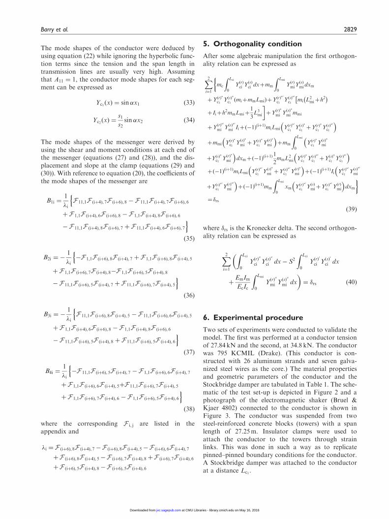
Two sets of experiments were conducted to validate themodel. The first was performed at a conductor tensionof 27.84 kN and the second, at 34.8 kN. The conductorwas 795 KCMIL (Drake). (This conductor is con-structed with 26 aluminum strands and seven galva-nized steel wires as the core.) The material propertiesand geometric parameters of the conductor and theStockbridge damper are tabulated in Table 1. The sche-matic of the test set-up is depicted in Figure 2 and aphotograph of the electromagnetic shaker (Bruel &Kjaer 4802) connected to the conductor is shown inFigure 3. The conductor was suspended from twosteel-reinforced concrete blocks (towers) with a spanlength of 27.25m. Insulator clamps were used toattach the conductor to the towers through strainlinks. This was done in such a way as to replicatepinned–pinned boundary conditions for the conductor.A Stockbridge damper was attached to the conductorat a distance Lc1 .

Barry et al. 2829



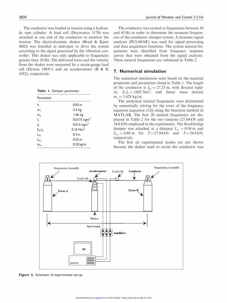
The conductor was loaded in tension using a hydrau-lic ram cylinder. A load cell (Daytronics 3170) wasattached at one end of the conductor to monitor thetension. The electrodynamic shaker (Bruel & Kjaer4802) was installed at mid-span to drive the systemaccording to the signal generated by the vibration con-troller. This shaker was only applicable to frequenciesgreater than 10 Hz. The delivered force and the velocityfrom the shaker were measured by a strain-gauge loadcell (Dytran 106V1) and an accelerometer (B & K4382), respectively.

The conductor was excited at frequencies between 10and 45Hz in order to determine the resonant frequen-cies of the conductor–damper system. A dynamic signalanalyzer (PCI-6034E) was used for signal processingand data acquisition functions. The system natural fre-quencies were identified from frequency responsecurves that were obtained from the signal analyzer.These natural frequencies are tabulated in Table 2.

7. Numerical simulation

The numerical simulations were based on the materialproperties and parameters listed in Table 1. The lengthof the conductor is Lc ¼ 27:25 m, with flexural rigid-ity EcIc ¼ 1602 Nm2, and linear mass densitymc ¼ 1:628 kg=m.

The analytical natural frequencies were determinedby numerically solving for the roots of the frequencyequation (equation (32)) using the bisection method inMATLAB. The first 20 natural frequencies are dis-played in Table 2 for the two tensions (27.84 kN and34.8 kN) employed in the experiments. The Stockbridgedamper was attached at a distance Lc1 ¼ 0:94 m andLc1 ¼ 0:88 m for T¼ 27.84 kN and T¼ 34.8 kN,respectively.

The first six experimental modes are not shownbecause the shaker used to excite the conductor was

Figure 2. Schematic of experimental set-up.

Table 1. Damper parameter.

Parameter

h 0.05 m

m1 3.4 kg

m2 1.46 kg

I1 0.0175 kgm2

I2 0.015 kgm2

EmIm 31.8 Nm2

Lm10.3 m

Lm20.22 m

mm 0.25 kg/m




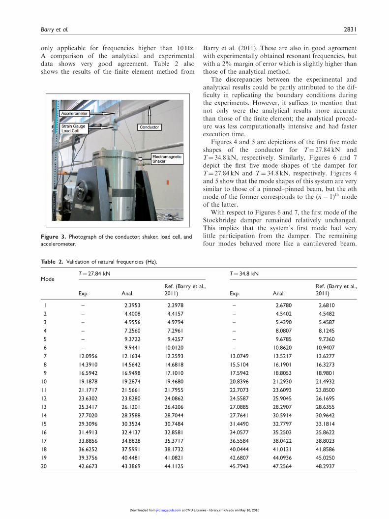
only applicable for frequencies higher than 10Hz.A comparison of the analytical and experimentaldata shows very good agreement. Table 2 alsoshows the results of the finite element method from

Barry et al. (2011). These are also in good agreementwith experimentally obtained resonant frequencies, butwith a 2% margin of error which is slightly higher thanthose of the analytical method.

The discrepancies between the experimental andanalytical results could be partly attributed to the dif-ficulty in replicating the boundary conditions duringthe experiments. However, it suffices to mention thatnot only were the analytical results more accuratethan those of the finite element; the analytical proced-ure was less computationally intensive and had fasterexecution time.

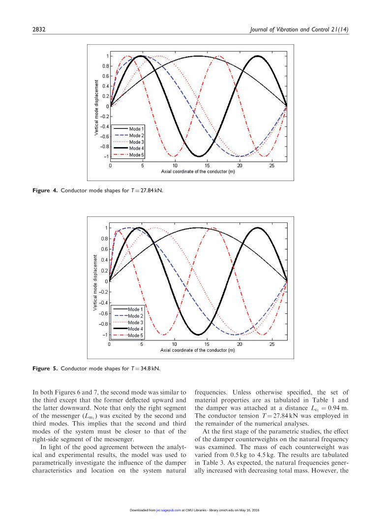
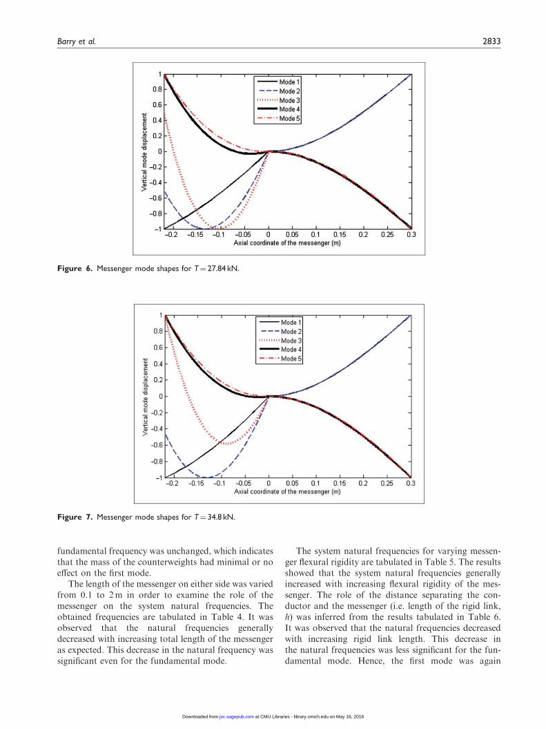
Figures 4 and 5 are depictions of the first five modeshapes of the conductor for T¼ 27.84 kN andT¼ 34.8 kN, respectively. Similarly, Figures 6 and 7depict the first five mode shapes of the damper forT¼ 27.84 kN and T¼ 34.8 kN, respectively. Figures 4and 5 show that the mode shapes of this system are verysimilar to those of a pinned–pinned beam, but the nthmode of the former corresponds to the ðn� 1Þth modeof the latter.

With respect to Figures 6 and 7, the first mode of theStockbridge damper remained relatively unchanged.This implies that the system’s first mode had verylittle participation from the damper. The remainingfour modes behaved more like a cantilevered beam.

Table 2. Validation of natural frequencies (Hz).

ModeT¼ 27.84 kN T¼ 34.8 kN

Exp. Anal.

Ref. (Barry et al.,

2011) Exp. Anal.

Ref. (Barry et al.,

2011)

1 – 2.3953 2.3978 – 2.6780 2.6810

2 – 4.4008 4.4157 – 4.5402 4.5482

3 – 4.9556 4.9794 – 5.4390 5.4587

4 – 7.2560 7.2961 – 8.0807 8.1245

5 – 9.3722 9.4257 – 9.6785 9.7360

6 – 9.9441 10.0120 – 10.8620 10.9407

7 12.0956 12.1634 12.2593 13.0749 13.5217 13.6277

8 14.3910 14.5642 14.6818 15.5104 16.1901 16.3273

9 16.5942 16.9498 17.1010 17.5942 18.8053 18.9801

10 19.1878 19.2874 19.4680 20.8396 21.2930 21.4932

11 21.1717 21.5661 21.7955 22.7073 23.6093 23.8500

12 23.6302 23.8280 24.0862 24.5587 25.9045 26.1695

13 25.3417 26.1201 26.4206 27.0885 28.2907 28.6355

14 27.7020 28.3588 28.7044 27.7641 30.5914 30.9642

15 29.3096 30.3524 30.7484 31.4490 32.7797 33.1814

16 31.4913 32.4137 32.8581 34.0577 35.2503 35.8622

17 33.8856 34.8828 35.3717 36.5584 38.0422 38.8023

18 36.6252 37.5991 38.1732 40.0444 41.0131 41.8586

19 39.3756 40.4481 41.0821 42.6807 44.0936 45.0250

20 42.6673 43.3869 44.1125 45.7943 47.2564 48.2937

Figure 3. Photograph of the conductor, shaker, load cell, and

accelerometer.

Barry et al. 2831



In both Figures 6 and 7, the second mode was similar tothe third except that the former deflected upward andthe latter downward. Note that only the right segmentof the messenger (Lm1

) was excited by the second andthird modes. This implies that the second and thirdmodes of the system must be closer to that of theright-side segment of the messenger.

In light of the good agreement between the analyt-ical and experimental results, the model was used toparametrically investigate the influence of the dampercharacteristics and location on the system natural

frequencies. Unless otherwise specified, the set ofmaterial properties are as tabulated in Table 1 andthe damper was attached at a distance Lc1 ¼ 0:94 m.The conductor tension T¼ 27.84 kN was employed inthe remainder of the numerical analyses.

At the first stage of the parametric studies, the effectof the damper counterweights on the natural frequencywas examined. The mass of each counterweight wasvaried from 0.5 kg to 4.5 kg. The results are tabulatedin Table 3. As expected, the natural frequencies gener-ally increased with decreasing total mass. However, the

Figure 4. Conductor mode shapes for T¼ 27.84 kN.

Figure 5. Conductor mode shapes for T¼ 34.8 kN.




fundamental frequency was unchanged, which indicatesthat the mass of the counterweights had minimal or noeffect on the first mode.

The length of the messenger on either side was variedfrom 0.1 to 2m in order to examine the role of themessenger on the system natural frequencies. Theobtained frequencies are tabulated in Table 4. It wasobserved that the natural frequencies generallydecreased with increasing total length of the messengeras expected. This decrease in the natural frequency wassignificant even for the fundamental mode.

The system natural frequencies for varying messen-ger flexural rigidity are tabulated in Table 5. The resultsshowed that the system natural frequencies generallyincreased with increasing flexural rigidity of the mes-senger. The role of the distance separating the con-ductor and the messenger (i.e. length of the rigid link,h) was inferred from the results tabulated in Table 6.It was observed that the natural frequencies decreasedwith increasing rigid link length. This decrease inthe natural frequencies was less significant for the fun-damental mode. Hence, the first mode was again

Figure 7. Messenger mode shapes for T¼ 34.8 kN.

Figure 6. Messenger mode shapes for T¼ 27.84 kN.

Barry et al. 2833



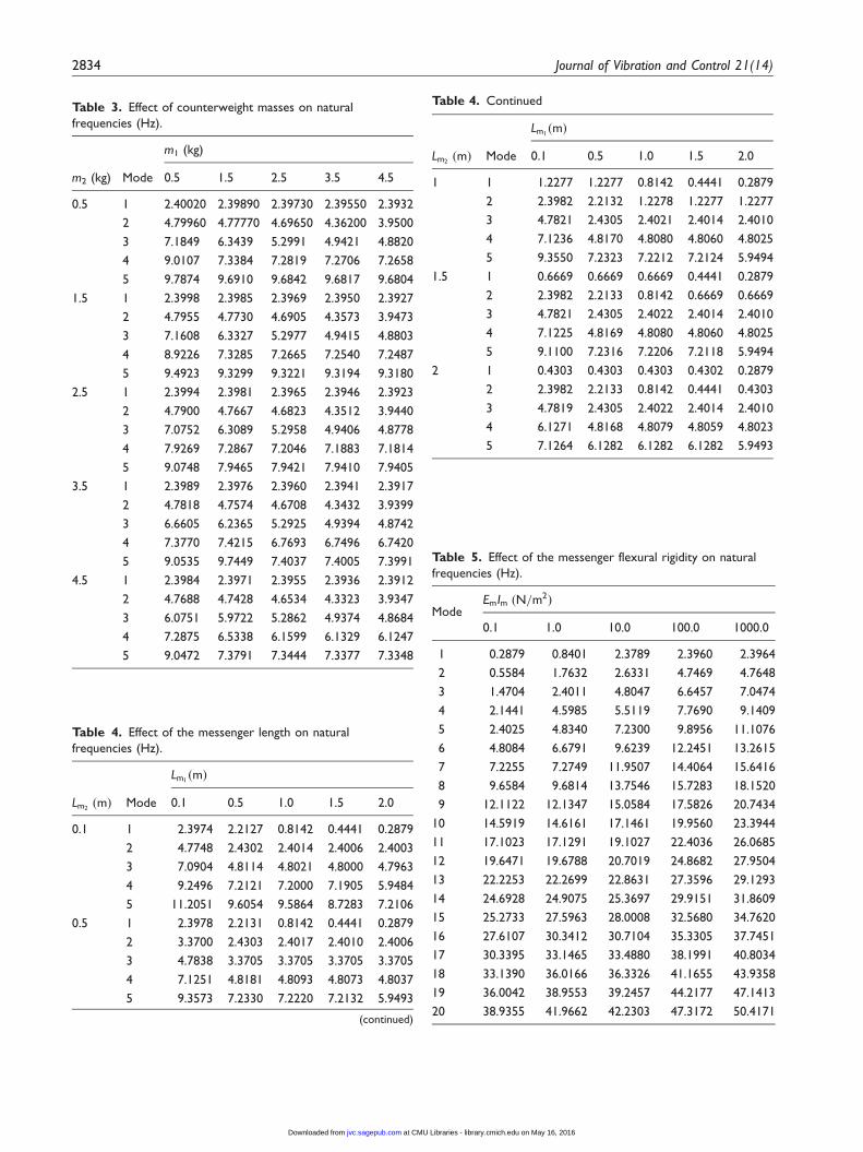
Table 3. Effect of counterweight masses on natural

frequencies (Hz).

m2 (kg) Mode

m1 (kg)

0.5 1.5 2.5 3.5 4.5

0.5 1 2.40020 2.39890 2.39730 2.39550 2.3932

2 4.79960 4.77770 4.69650 4.36200 3.9500

3 7.1849 6.3439 5.2991 4.9421 4.8820

4 9.0107 7.3384 7.2819 7.2706 7.2658

5 9.7874 9.6910 9.6842 9.6817 9.6804

1.5 1 2.3998 2.3985 2.3969 2.3950 2.3927

2 4.7955 4.7730 4.6905 4.3573 3.9473

3 7.1608 6.3327 5.2977 4.9415 4.8803

4 8.9226 7.3285 7.2665 7.2540 7.2487

5 9.4923 9.3299 9.3221 9.3194 9.3180

2.5 1 2.3994 2.3981 2.3965 2.3946 2.3923

2 4.7900 4.7667 4.6823 4.3512 3.9440

3 7.0752 6.3089 5.2958 4.9406 4.8778

4 7.9269 7.2867 7.2046 7.1883 7.1814

5 9.0748 7.9465 7.9421 7.9410 7.9405

3.5 1 2.3989 2.3976 2.3960 2.3941 2.3917

2 4.7818 4.7574 4.6708 4.3432 3.9399

3 6.6605 6.2365 5.2925 4.9394 4.8742

4 7.3770 7.4215 6.7693 6.7496 6.7420

5 9.0535 9.7449 7.4037 7.4005 7.3991

4.5 1 2.3984 2.3971 2.3955 2.3936 2.3912

2 4.7688 4.7428 4.6534 4.3323 3.9347

3 6.0751 5.9722 5.2862 4.9374 4.8684

4 7.2875 6.5338 6.1599 6.1329 6.1247

5 9.0472 7.3791 7.3444 7.3377 7.3348

Table 5. Effect of the messenger flexural rigidity on natural

frequencies (Hz).

ModeEmIm ðN=m

2Þ

0.1 1.0 10.0 100.0 1000.0

1 0.2879 0.8401 2.3789 2.3960 2.3964

2 0.5584 1.7632 2.6331 4.7469 4.7648

3 1.4704 2.4011 4.8047 6.6457 7.0474

4 2.1441 4.5985 5.5119 7.7690 9.1409

5 2.4025 4.8340 7.2300 9.8956 11.1076

6 4.8084 6.6791 9.6239 12.2451 13.2615

7 7.2255 7.2749 11.9507 14.4064 15.6416

8 9.6584 9.6814 13.7546 15.7283 18.1520

9 12.1122 12.1347 15.0584 17.5826 20.7434

10 14.5919 14.6161 17.1461 19.9560 23.3944

11 17.1023 17.1291 19.1027 22.4036 26.0685

12 19.6471 19.6788 20.7019 24.8682 27.9504

13 22.2253 22.2699 22.8631 27.3596 29.1293

14 24.6928 24.9075 25.3697 29.9151 31.8609

15 25.2733 27.5963 28.0008 32.5680 34.7620

16 27.6107 30.3412 30.7104 35.3305 37.7451

17 30.3395 33.1465 33.4880 38.1991 40.8034

18 33.1390 36.0166 36.3326 41.1655 43.9358

19 36.0042 38.9553 39.2457 44.2177 47.1413

20 38.9355 41.9662 42.2303 47.3172 50.4171

Table 4. Effect of the messenger length on natural

frequencies (Hz).

Lm2ðmÞ Mode

Lm1ðmÞ

0.1 0.5 1.0 1.5 2.0

0.1 1 2.3974 2.2127 0.8142 0.4441 0.2879

2 4.7748 2.4302 2.4014 2.4006 2.4003

3 7.0904 4.8114 4.8021 4.8000 4.7963

4 9.2496 7.2121 7.2000 7.1905 5.9484

5 11.2051 9.6054 9.5864 8.7283 7.2106

0.5 1 2.3978 2.2131 0.8142 0.4441 0.2879

2 3.3700 2.4303 2.4017 2.4010 2.4006

3 4.7838 3.3705 3.3705 3.3705 3.3705

4 7.1251 4.8181 4.8093 4.8073 4.8037

5 9.3573 7.2330 7.2220 7.2132 5.9493

(continued)

Table 4. Continued

Lm2ðmÞ Mode

Lm1ðmÞ

0.1 0.5 1.0 1.5 2.0

1 1 1.2277 1.2277 0.8142 0.4441 0.2879

2 2.3982 2.2132 1.2278 1.2277 1.2277

3 4.7821 2.4305 2.4021 2.4014 2.4010

4 7.1236 4.8170 4.8080 4.8060 4.8025

5 9.3550 7.2323 7.2212 7.2124 5.9494

1.5 1 0.6669 0.6669 0.6669 0.4441 0.2879

2 2.3982 2.2133 0.8142 0.6669 0.6669

3 4.7821 2.4305 2.4022 2.4014 2.4010

4 7.1225 4.8169 4.8080 4.8060 4.8025

5 9.1100 7.2316 7.2206 7.2118 5.9494

2 1 0.4303 0.4303 0.4303 0.4302 0.2879

2 2.3982 2.2133 0.8142 0.4441 0.4303

3 4.7819 2.4305 2.4022 2.4014 2.4010

4 6.1271 4.8168 4.8079 4.8059 4.8023

5 7.1264 6.1282 6.1282 6.1282 5.9493




dominated by the conductor characteristics. Table 7shows the influence of the location of the Stockbridgedamper on the system natural frequencies. The locationof the damper affected all five modes, but with no obvi-ous trend.

8. Conclusions

A double-beam-concept-based analytical model waspresented for the free vibration analysis of a single con-ductor transmission line with a Stockbridge damper forthe first time. The first or main beam was subjected toan axial load and had pinned–pinned boundary condi-tions in order to simulate single conductor transmissionlines on suspension-spans. The Stockbridge damperwas modeled by an in-span beam with tip mass ateach end. The model was validated experimentally.Expressions were presented for the frequency equation,mode shapes, and orthogonality relations. Experimentswere conducted to validate the proposed model and theresults showed very good agreement.

Parametric investigations indicated that the mass ofthe counterweights, length of the rigid link, length ofthe messenger, and flexural rigidity had more effect onthe higher modes. The first mode was dominated by theconductor characteristics. The role of the location ofthe Stockbridge damper with respect to the system nat-ural frequencies was inconclusive.

Acknowledgments

The authors are grateful to Andrew Rizzetto and DmitryLadin of Kinectrics Inc., Toronto, for their assistance withthe experiments.

Funding

The financial assistance from Hydro One Inc. is

acknowledged.

References

Abu-Hilal M (2006) Dynamic response of a double Euler-

Bernoulli beam due to a moving constant load. Journal

of Sound and Vibration 297: 477–491.

Barry O, Oguamanam DCD and Lin DC (2011) Free vibra-

tion analysis of a single conductor with a Stockbridge

Table 6. Effect of clamp height on natural frequencies (Hz).

Mode

h (m)

0.01 0.5 1.0 1.5 2.0

1 2.3950 2.3940 2.3907 2.3840 2.3713

2 4.3574 4.3452 4.2975 4.1569 3.7714

3 4.9415 4.9409 4.9385 4.9307 4.8745

4 7.2541 7.2371 7.0962 5.9075 5.0666

5 9.3194 9.3167 8.5572 7.4561 7.3783

6 9.9127 9.8458 9.3371 9.3269 9.3257

7 12.1632 12.0116 10.3493 10.1209 10.0857

8 14.5646 14.2654 12.5256 12.4019 12.3754

9 16.9490 16.4393 14.8943 14.8146 14.7947

10 19.2828 18.5509 17.2439 17.1882 17.1731

11 21.5550 20.3939 19.4821 19.4509 19.4421

12 23.8115 21.7886 21.6128 21.6056 21.6034

13 26.1005 23.8115 23.8115 23.8115 23.8115

14 28.3314 26.1456 26.1265 26.1246 26.1240

15 30.3150 28.3625 28.3521 28.3509 28.3505

16 32.3899 30.3337 30.3287 30.3281 30.3278

17 34.8730 32.5772 32.5357 32.5300 32.5281

18 37.5963 35.1854 35.1246 35.1158 35.1128

19 40.4486 37.9646 37.8995 37.8898 37.8866

20 43.3881 40.8243 40.7631 40.7538 40.7507

Table 7. Effect of damper location on natural frequencies (Hz).

Mode

Lc1

Lc=100 Lc=10 Lc=6 Lc=4 Lc=2

1 2.3999 2.3614 2.3049 2.2288 2.1201

2 4.5444 4.0203 3.9004 3.9544 4.7092

3 4.8621 5.1583 5.3589 5.4976 4.8423

4 7.2383 7.1893 7.0885 7.0926 7.0949

5 9.6696 8.8023 9.0209 9.6194 9.6104

6 12.1225 10.3922 10.7470 12.2225 9.8972

7 14.5983 14.5833 12.2794 14.5632 12.4048

8 17.0988 16.9846 14.6115 17.0170 14.6111

9 19.6190 19.5491 17.0247 19.6732 16.8610

10 22.1239 22.2159 19.2416 21.7401 19.6731

11 24.3187 24.8734 21.6055 23.9078 21.5417

12 25.6735 25.8659 24.3172 26.7988 24.8785

13 27.8490 27.8460 27.0319 27.9871 25.7063

14 30.4769 30.5062 27.7439 30.3646 28.3762

15 33.1860 32.6745 30.3640 32.9017 30.3669

16 35.7006 34.7148 33.1236 34.7440 32.4379

17 37.1094 37.4496 34.7936 38.0303 36.0100

18 39.3438 40.4795 37.3504 41.5599 37.0541

(continued)

Table 7. Continued

Mode

Lc1

Lc=100 Lc=10 Lc=6 Lc=4 Lc=2

19 42.2444 43.6002 40.5902 42.1458 41.4734

20 45.2944 46.6673 42.2288 45.5969 42.0975

Barry et al. 2835



damper. In: Proceedings of the 23rd CANCAM,

Vancouver, BC, 5–9 June 2011.

Barry O, Oguamanam DCD and Lin DC (2013) Aeolian

vibration of a single conductor with a Stockbridge

damper. IMechE: Part C, Journal of Mechanical

Engineering Science 227(5): 935–945.Chan JK and Lu ML (2007) An efficient algorithm for

Aeolian vibration of single conductor with multiple dam-

pers. Institute of Electrical and Electronics Engineers,

Transactions on Power Delivery 22(3): 1822–1829.Claren R and Diana G (1969) Mathematical analysis of trans-

mission line vibration. Institute of Electrical and

Electronics Engineers, Transactions on Power Apparatus

and Systems 60(2): 1741–1771.Dhotard MS, Ganesan N and Rao BVA (1978) Transmission

line vibration. Journal of Sound and Vibration 60(2):

217–237.

Foda MA (2009) Control of lateral vibrations and slopes at

desired locations along vibrating beams. Journal of

Vibration and Control 15(11): 1649–1678.Foda MA (2013) Transverse vibration control of translating

visco-elastically connected double-string-like continua.

Journal of Vibration and Control 19(9): 1316–1332.Kraus M and Hagedorn P (1991) Aeolian vibration: Wind

energy input evaluated from measurements on an ener-

gized transmission lines. Institute of Electrical and

Electronics Engineers, Transactions on Power Delivery

6(3): 1264–1270.Nigol O and Houston HJ (1985) Aeolian vibration of single

conductor and its control. Institute of Electrical and

Electronics Engineers, Transactions on Power Apparatusand Systems 104(11): 3245–3254.

Oguamanam DCD, Hansen JS and Heppler GR (1998)

Vibration of arbitrarily oriented two-member openframes with tip mass. Journal of Sound and Vibration209(4): 651–669.

Oniszczuk Z (2000) Free transverse vibration of elastically

connected simply supported double-beam complexsystem. Journal of Sound and Vibration 232: 387–403.

Oniszczuk Z (2003) Forced transverse vibrations of an elas-

tically connected complex simply supported double-beamsystem. Journal of Sound and Vibration 264: 273–286.

Palmeri A and Adhikari S (2011) A Galerkin-type state-space

approach for transverse vibrations of slender double-beamsystems with viscoelastic inner layer. Journal of Sound andVibration 330: 6372–6386.

Vecchiarelly J, Curries IG and Havard DG (2000)Computational analysis of Aeolian conductor vibrationwith a Stockbridge-type damper. Journal of Fluid andStructures 14: 489–509.

Verma H and Hagerdorn P (2004) Wind induced vibration oflong electrical overhead transmission line spans: A mod-ified approach. Journal of Wind and Structures 8(2):

89–106.Vu HV, Ordonez AM and Karnopp BH (2000) Vibration of a

double-beam system. Journal of Sound and Vibration

229(4): 807–882.Yamaguchi H (1984) Vibration of a beam with an absorber

consisting of a viscoelastic beam and a spring-viscousdamper. Journal of Sound and Vibration 103(3): 417–425.

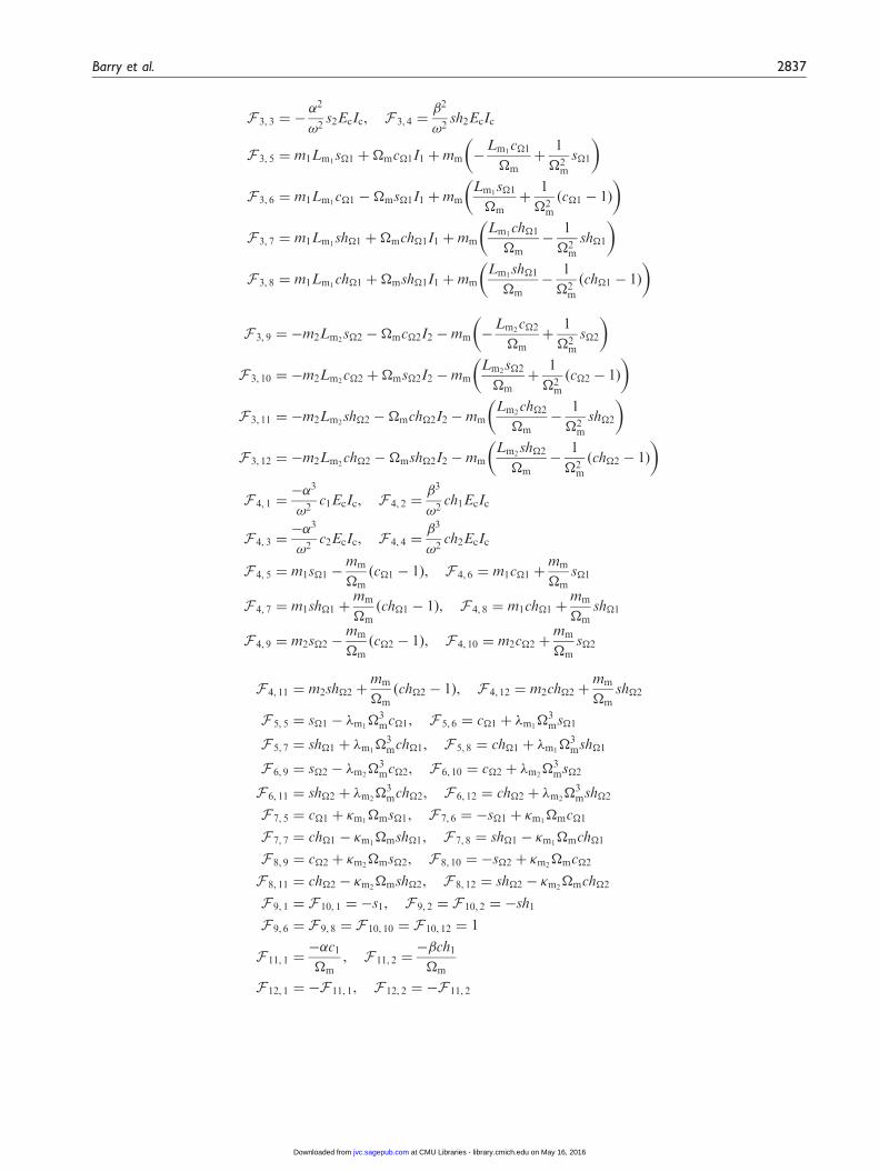
Appendix

For the sake of simplicity, the following notation is used:

si ¼ sin �Lci , shi ¼ sinh�Lci

ci ¼ cos�Lci , chi ¼ cosh�Lci

s�i ¼ sin�mLmi, sh�i ¼ sinh�mLmi

c�i ¼ cos�mLmi, ch�i ¼ sinh�mLmi

Matrix ½F i, j� comprises 144 elements in which 80 are zero entries and the remaining 64 elements are given as

F 1, 1 ¼ s1, F 1, 2 ¼ sh1, F 1, 3 ¼ �s2, F 1, 1 ¼ �sh2

F 2, 1 ¼ �c1, F 2, 2 ¼ �ch1, F 2, 3 ¼ �c2, F 2, 4 ¼ �ch2

F 3, 1 ¼ �c1h2 m1 þm2 þmm1

þmm2

� �þ�2

!2EcIcs1

F 3, 2 ¼ �ch1h2 m1 þm2 þmm1

þmm2

� ��2

!2EcIcsh1




F 3, 3 ¼ ��2

!2s2EcIc, F 3, 4 ¼

�2

!2sh2EcIc

F 3, 5 ¼ m1Lm1s�1 þ�mc�1I1 þmm �

Lm1c�1

�mþ

1

�2m

s�1

� �

F 3, 6 ¼ m1Lm1c�1 ��ms�1I1 þmm

Lm1s�1

�mþ

1

�2m

ðc�1 � 1Þ

� �

F 3, 7 ¼ m1Lm1sh�1 þ�mch�1I1 þmm

Lm1ch�1

�m�

1

�2m

sh�1

� �

F 3, 8 ¼ m1Lm1ch�1 þ�msh�1I1 þmm

Lm1sh�1

�m�

1

�2m

ðch�1 � 1Þ

� �

F 3, 9 ¼ �m2Lm2s�2 ��mc�2I2 �mm �

Lm2c�2

�mþ

1

�2m

s�2

� �

F 3, 10 ¼ �m2Lm2c�2 þ�ms�2I2 �mm

Lm2s�2

�mþ

1

�2m

ðc�2 � 1Þ

� �

F 3, 11 ¼ �m2Lm2sh�2 ��mch�2I2 �mm

Lm2ch�2

�m�

1

�2m

sh�2

� �

F 3, 12 ¼ �m2Lm2ch�2 ��msh�2I2 �mm

Lm2sh�2

�m�

1

�2m

ðch�2 � 1Þ

� �

F 4, 1 ¼��3

!2c1EcIc, F 4, 2 ¼

�3

!2ch1EcIc

F 4, 3 ¼��3

!2c2EcIc, F 4, 4 ¼

�3

!2ch2EcIc

F 4, 5 ¼ m1s�1 �mm

�mðc�1 � 1Þ, F 4, 6 ¼ m1c�1 þ

mm

�ms�1

F 4, 7 ¼ m1sh�1 þmm

�mðch�1 � 1Þ, F 4, 8 ¼ m1ch�1 þ

mm

�msh�1

F 4, 9 ¼ m2s�2 �mm

�mðc�2 � 1Þ, F 4, 10 ¼ m2c�2 þ

mm

�ms�2

F 4, 11 ¼ m2sh�2 þmm

�mðch�2 � 1Þ, F 4, 12 ¼ m2ch�2 þ

mm

�msh�2

F 5, 5 ¼ s�1 � �m1�3

mc�1, F 5, 6 ¼ c�1 þ �m1�3

ms�1

F 5, 7 ¼ sh�1 þ �m1�3

mch�1, F 5, 8 ¼ ch�1 þ �m1�3

msh�1

F 6, 9 ¼ s�2 � �m2�3

mc�2, F 6, 10 ¼ c�2 þ �m2�3

ms�2

F 6, 11 ¼ sh�2 þ �m2�3

mch�2, F 6, 12 ¼ ch�2 þ �m2�3

msh�2

F 7, 5 ¼ c�1 þ �m1�ms�1, F 7, 6 ¼ �s�1 þ �m1

�mc�1

F 7, 7 ¼ ch�1 � �m1�msh�1, F 7, 8 ¼ sh�1 � �m1

�mch�1

F 8, 9 ¼ c�2 þ �m2�ms�2, F 8, 10 ¼ �s�2 þ �m2

�mc�2

F 8, 11 ¼ ch�2 � �m2�msh�2, F 8, 12 ¼ sh�2 � �m2

�mch�2

F 9, 1 ¼ F 10, 1 ¼ �s1, F 9, 2 ¼ F 10, 2 ¼ �sh1

F 9, 6 ¼ F 9, 8 ¼ F 10, 10 ¼ F 10, 12 ¼ 1

F 11, 1 ¼��c1�m

, F 11, 2 ¼��ch1

�m

F 12, 1 ¼ �F 11, 1, F 12, 2 ¼ �F 11, 2

Barry et al. 2837



Documents

Analytical and experimental investigation The Author(s ...people.cst.cmich.edu/barry1o/assets/pdf/Analytical_and... · Article Analytical and experimental investigation of overhead