Embed Size (px)
Citation preview
Analysis of Three-Way Contingency Table
CF Jeff Lin, MD., PhD.
March 14, 2006
c©Jeff Lin, MD., PhD.

Analysis of Three-Way Contingency Table
c©Jeff Lin, MD., PhD. Three-Way Table, 1
Analysis of Three-Way Contingency Table
1. An important of any research study is the choice of predictor and
control variables.
2. Unless we include relevant variables in the analysis, result will have
limited usefulness.
3. In study relationship between a response variable and an explanatory
variable, we should control covariates that can influence that
relationship.
c©Jeff Lin, MD., PhD. Three-Way Table, 2

Analysis of Three-Way Contingency Table
1. For instance, we are studying effects of passive smoking-the effects on
non-smoker of living with a smoker. We might compare lung cancer
rates between non-smokers whose spouses smoke and non-smokers
whose spouses do not smoke.
2. In doing so, we should control for age, work environment,
socioeconomic status, or other factors that might relate both to
whether one’s spouse smokers and to whether one has lung cancer.
c©Jeff Lin, MD., PhD. Three-Way Table, 3

Death Penalty Example
1. Table 1 (Table 3.1, page 54, Agresti’s Introduction, 1996) is a
2× 2× 2 contingency table–two rows, two columns, and two
layers–from an article that studied effects of racial characteristics on
whether persons convicted of homicide received the death penalty.
2. The 674 subjects classified in Table 1 were the defendants in
indictments involving cases with multiple murders in Florida between
1976 and 1987.
c©Jeff Lin, MD., PhD. Three-Way Table, 4

Death Penalty Example
3. The variables in Table 1 are Y = death penalty verdict, having the
categories (yes, no), X = race of defendant, and Z = race of victims,
each having the categories (white, black).
4. We study the effect of defendant’s race on the death penalty verdict,
treating victims’ race are a control variable.
5. Table 1 has a 2× 2 partial table relating defendant’s rance and the
death penalty verdict at each category of victims’ race.
c©Jeff Lin, MD., PhD. Three-Way Table, 5

Table 1: Death Penalty Verdict by Defendant’s
Race and Victims’ Race
Victims’ Defendant’s Death Penalty Percent
Race Race Yes No Yes
White White 53 424 11.3
Black 11 37 22.9
Black White 0 16 0.0
Bkack 4 139 2.8
Total White 53 430 11.0
Black 15 176 7.9
c©Jeff Lin, MD., PhD. Three-Way Table, 6
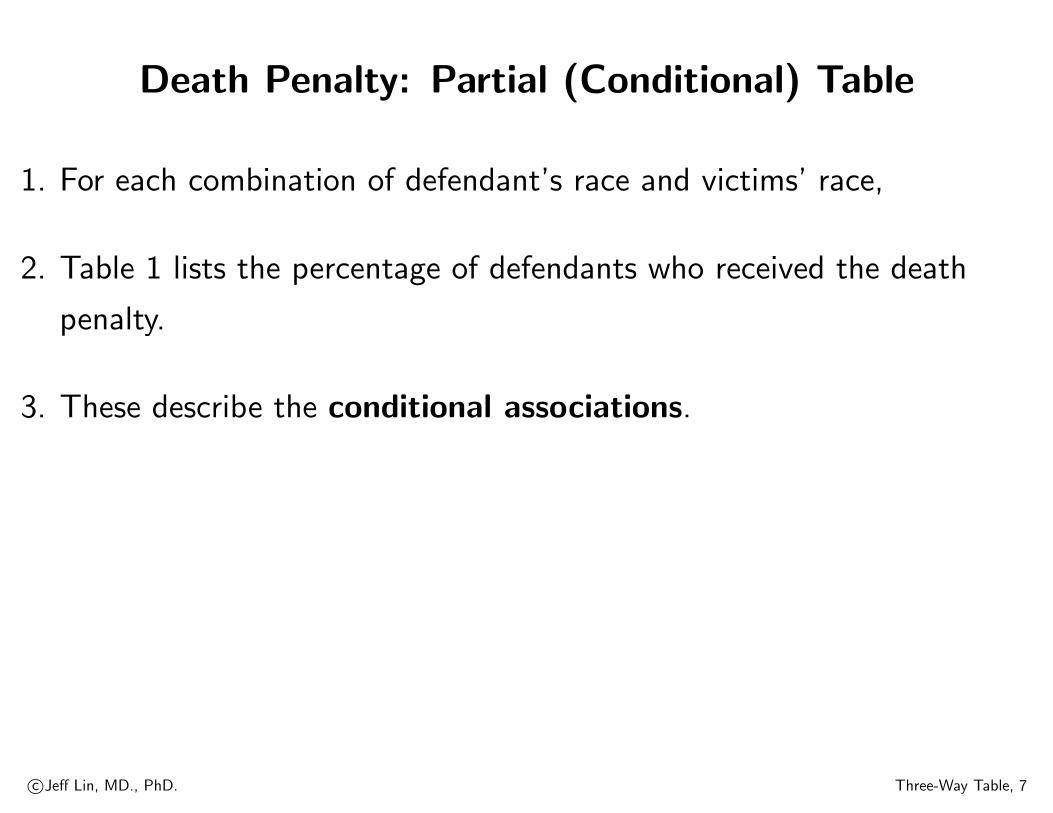
Death Penalty: Partial (Conditional) Table
1. For each combination of defendant’s race and victims’ race,
2. Table 1 lists the percentage of defendants who received the death
penalty.
3. These describe the conditional associations.
c©Jeff Lin, MD., PhD. Three-Way Table, 7
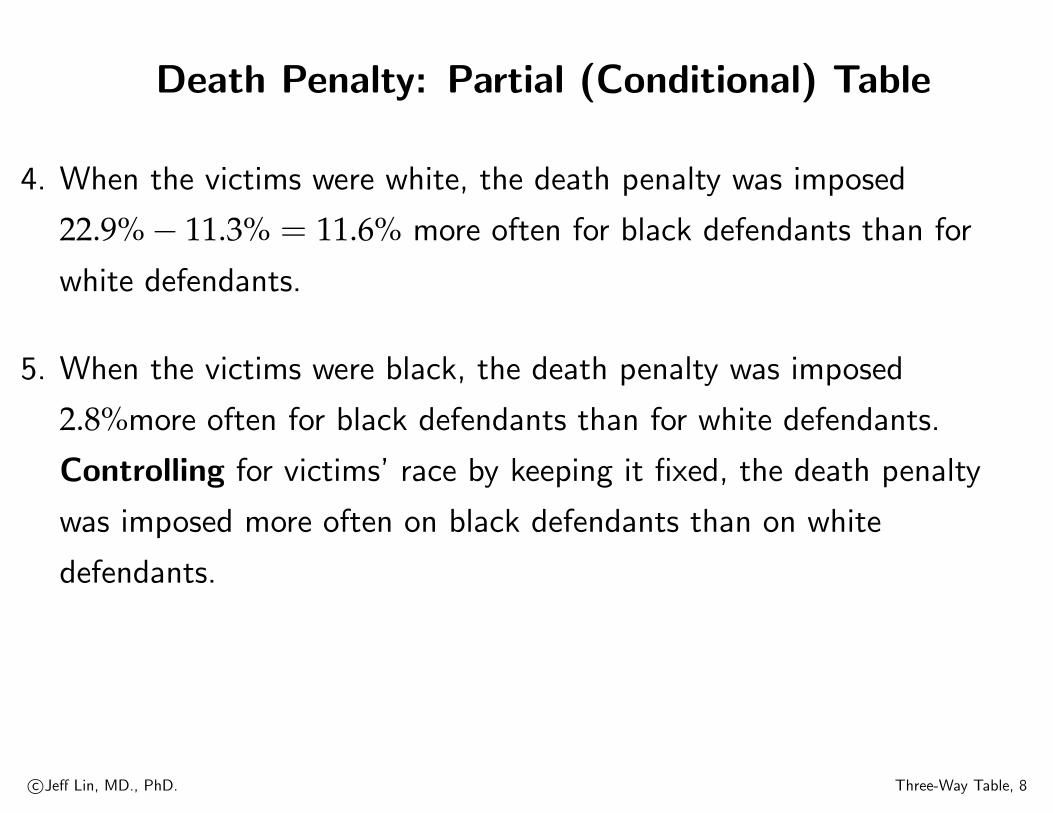
Death Penalty: Partial (Conditional) Table
4. When the victims were white, the death penalty was imposed
22.9%− 11.3% = 11.6% more often for black defendants than for
white defendants.
5. When the victims were black, the death penalty was imposed
2.8%more often for black defendants than for white defendants.
Controlling for victims’ race by keeping it fixed, the death penalty
was imposed more often on black defendants than on white
defendants.
c©Jeff Lin, MD., PhD. Three-Way Table, 8
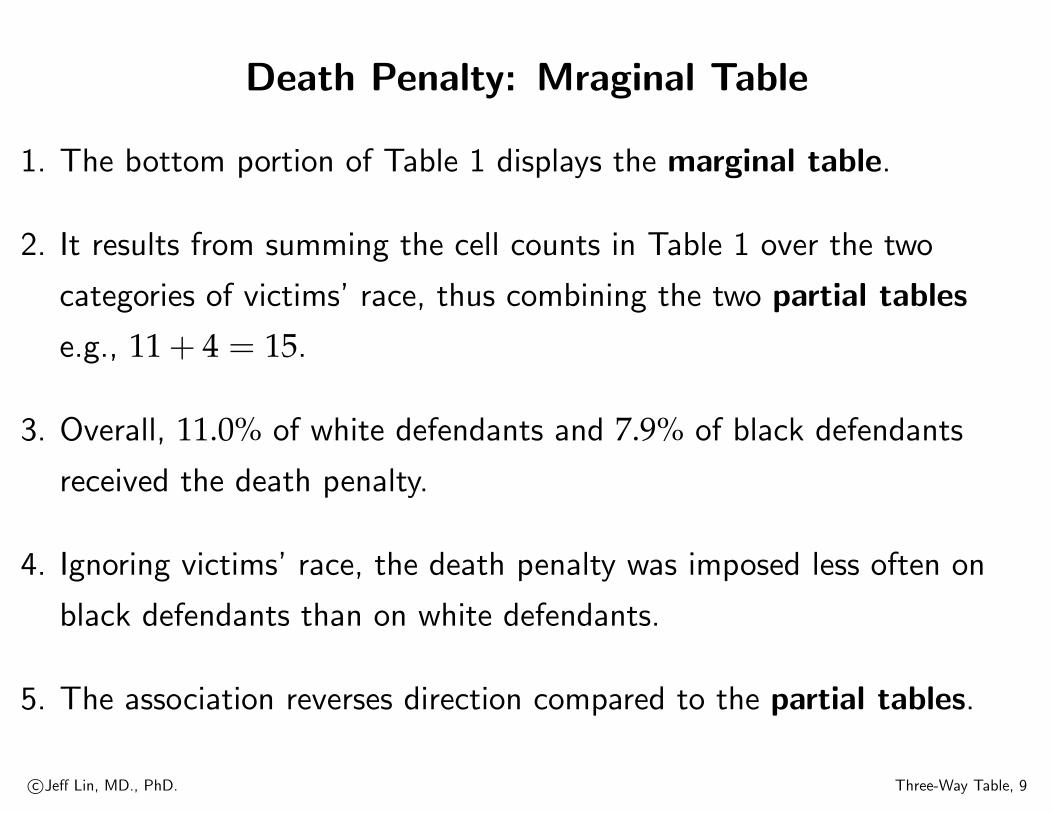
Death Penalty: Mraginal Table
1. The bottom portion of Table 1 displays the marginal table.
2. It results from summing the cell counts in Table 1 over the two
categories of victims’ race, thus combining the two partial tables
e.g., 11 + 4 = 15.
3. Overall, 11.0% of white defendants and 7.9% of black defendants
received the death penalty.
4. Ignoring victims’ race, the death penalty was imposed less often on
black defendants than on white defendants.
5. The association reverses direction compared to the partial tables.
c©Jeff Lin, MD., PhD. Three-Way Table, 9
Death Penalty: Results
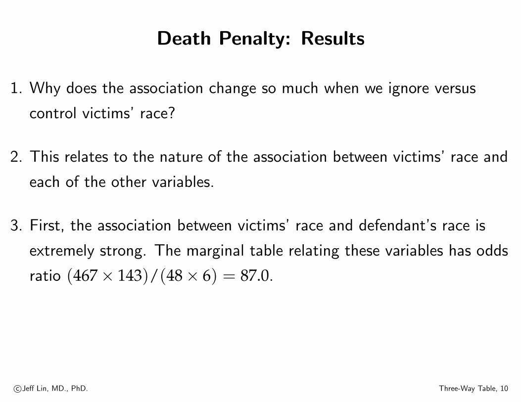
1. Why does the association change so much when we ignore versus
control victims’ race?
2. This relates to the nature of the association between victims’ race and
each of the other variables.
3. First, the association between victims’ race and defendant’s race is
extremely strong. The marginal table relating these variables has odds
ratio (467× 143)/(48× 6) = 87.0.
c©Jeff Lin, MD., PhD. Three-Way Table, 10

Death Penalty: Results
4. Second, Table 1 shows that, regardless of defendant’s race, the death
penalty was much more likely when the victims were white than when
the victims were black.
5. So whites are tending to kill whites, and killing whites is more likely to
result in the death penalty.
6. This suggests that the marginal association should show a greater
tendency than the conditional associations for white defendants to
receive the death penalty.
7. In fact, Table 1 has this pattern.
c©Jeff Lin, MD., PhD. Three-Way Table, 11

Death Penalty: Simpson’s paradox
1. The result that a marginal association can have a different direction
from each conditional association is called Simpson’s paradox
(Simpson 1951, Yule. 1903).
2. It applies to quantitative as well as categorical variables.
3. Statisticians commonly use it to caution against imputing causal
effects from an association of X with Y.
c©Jeff Lin, MD., PhD. Three-Way Table, 12

Death Penalty: Simpson’s paradox
4. For instance, when doctors started to observe strong odds ratios
between smoking and lung cancer, statisticians such as R. A. Fisher
warned that some variable e.g., a genetic factor could exist such that
the association would disappear under the relevant control.
5. However, other statisticians such as J. Cornfield showed that with a
very strong XY association, a very strong association must exist
between the confounding variable Z and both X and Y in order for
the effect to disappear or change under the control (Breslow and Day
1980, Sec. 3.4)
c©Jeff Lin, MD., PhD. Three-Way Table, 13

Three-Way Table
1. Suppose that we have three categorical variables, A, B, C, where Atakes possible value 1, 2, . . . I, B takes possible value 1, 2, . . . , J, Ctakes possible values 1, 2, . . . , K.
2. We display the distribution of A× B cell counts without considering
the different levels of C using cross sections of the two-way
contingency table A× B, we called it is a A× B marginal table.
(We ignore the existence of C.)
3. When we display the distribution of A× B cell counts at different
levels of C using cross sections of the three-way contingency table.
c©Jeff Lin, MD., PhD. Three-Way Table, 14

Three-Way Table: Partial Table and Marginal Table
1. The cross sections are called partial tables. In the partial table, C is
controlled; that is, its value is held constant.
2. The two-way contingency table obtained by combing the partial tables
is called the A− B marginal table. That table, rather controlling C,
ignore it.
3. Partial table can exhibit quite different associations than marginal
tables.
4. In fact, it can be misleading to analyze only the marginal tables of a
multi-way table.
c©Jeff Lin, MD., PhD. Three-Way Table, 15
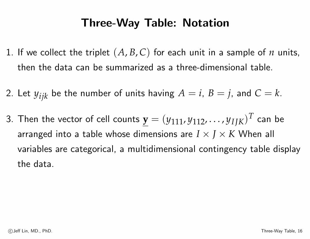
Three-Way Table: Notation
1. If we collect the triplet (A, B, C) for each unit in a sample of n units,
then the data can be summarized as a three-dimensional table.
2. Let yijk be the number of units having A = i, B = j, and C = k.
3. Then the vector of cell counts y = (y111, y112, . . . , yI JK)T can be
arranged into a table whose dimensions are I × J × K When all
variables are categorical, a multidimensional contingency table display
the data.
c©Jeff Lin, MD., PhD. Three-Way Table, 16
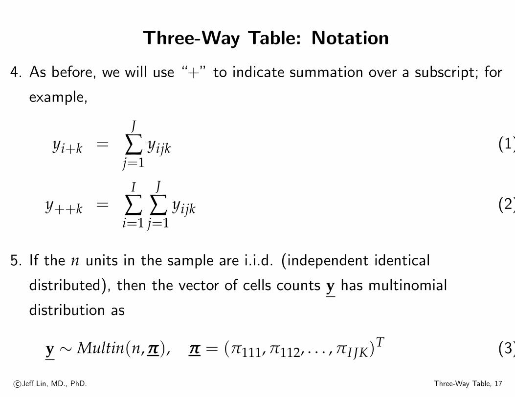
Three-Way Table: Notation
4. As before, we will use “+” to indicate summation over a subscript; for
example,
yi+k =J
∑j=1
yijk (1)
y++k =I
∑i=1
J
∑j=1
yijk (2)
5. If the n units in the sample are i.i.d. (independent identical
distributed), then the vector of cells counts y has multinomial
distribution as
y ∼ Multin(n, πππ), πππ = (π111, π112, . . . , πI JK)T (3)
c©Jeff Lin, MD., PhD. Three-Way Table, 17
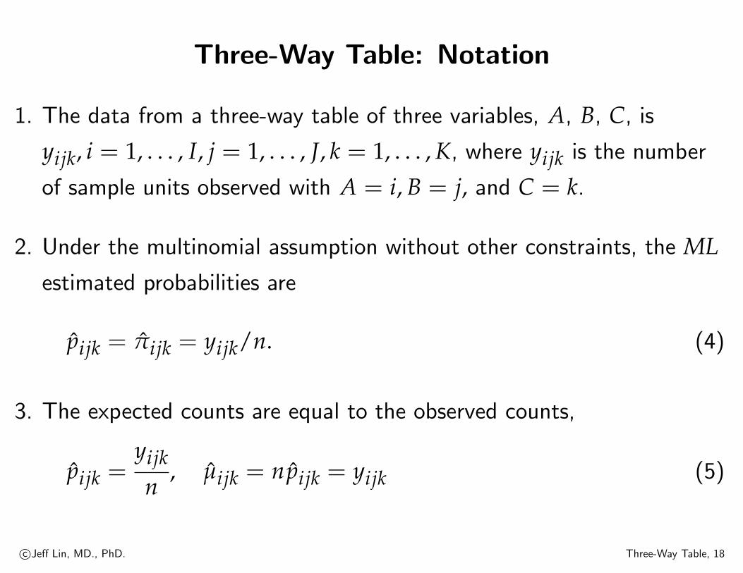
Three-Way Table: Notation
1. The data from a three-way table of three variables, A, B, C, is
yijk, i = 1, . . . , I, j = 1, . . . , J, k = 1, . . . , K, where yijk is the number
of sample units observed with A = i, B = j, and C = k.
2. Under the multinomial assumption without other constraints, the MLestimated probabilities are
pijk = πijk = yijk/n. (4)
3. The expected counts are equal to the observed counts,
pijk =yijk
n, µijk = npijk = yijk (5)
c©Jeff Lin, MD., PhD. Three-Way Table, 18
Three-Way Table: Notation
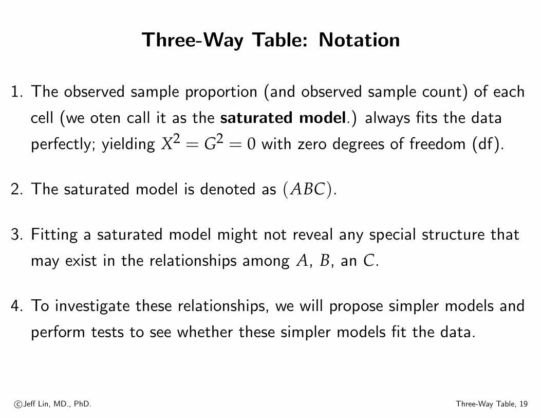
1. The observed sample proportion (and observed sample count) of each
cell (we oten call it as the saturated model.) always fits the data
perfectly; yielding X2 = G2 = 0 with zero degrees of freedom (df).
2. The saturated model is denoted as (ABC).
3. Fitting a saturated model might not reveal any special structure that
may exist in the relationships among A, B, an C.
4. To investigate these relationships, we will propose simpler models and
perform tests to see whether these simpler models fit the data.
c©Jeff Lin, MD., PhD. Three-Way Table, 19

Three-Way Table: Types of Independence
c©Jeff Lin, MD., PhD. Three-Way Table, 20

Types of Independence
1. Complete Independence
2. Joint Independent
3. Conditional Independence
4. Homogeneous Association
5. Saturated
c©Jeff Lin, MD., PhD. Three-Way Table, 21

Complete Independence
c©Jeff Lin, MD., PhD. Three-Way Table, 22

Types of Independence: Complete Independence
The simplest model that one night propose is
πijk = P(A = i, B = j, C = k) (6)
= P(A = i)P(B = j)P(C = k), (7)
= πi++π+j+π++k, for all i, j, k. (8)
c©Jeff Lin, MD., PhD. Three-Way Table, 23

Complete Independence
Define
αi = P(A = i), i = 1, 2, . . . , I (9)
β j = P(B = j), j = 1, 2, . . . , J (10)
γk = P(C = k), k = 1, 2, . . . , K (11)
so that πijk = αiβ jγk, for all i, j, k. The unknown parameters are
α = (α1, α2, . . . , αI)T, β = (β1, β2, . . . , β J)
T, γ = (γ1, γ2, . . . , γK)T(12)
c©Jeff Lin, MD., PhD. Three-Way Table, 24

Complete Independence: Sampling Distribution
1. Because each of these vectors must add up to one, the number of free
parameters in the model is (I − 1) + (J − 1) + (K − 1). Notice that
under the complete independent model,
(y1++, y2++, . . . , yI++) ∼ Multin(n, α) (13)
(y+1+, y+2+, . . . , y+J+) ∼ Multin(n, β) (14)
(y++1, y++2, . . . , y++J) ∼ Multin(n, γ) (15)
2. These three vectors are mutually independent.
3. Thus the three parameter vector ααα, βββ, and γγγ can be estimated
independence of one another.
c©Jeff Lin, MD., PhD. Three-Way Table, 25

Complete Independence: Point Estimation
The ML estimates are given by
αi = yi++/n, i = 1, 2, . . . , I (16)
β j = y+j+/n, j = 1, 2, . . . , J (17)
γk = y++k/n, k = 1, 2, . . . , K (18)
(19)
Under complete independence, ML estimates of the expected cell
frequencies are mutually independence as
µ0ijk = nαiβiγk =
yi++ y+j+ y++k
n2 (20)
The number of free parameters in this model is
(I − 1) + (J − 1) + (K − 1).
c©Jeff Lin, MD., PhD. Three-Way Table, 26
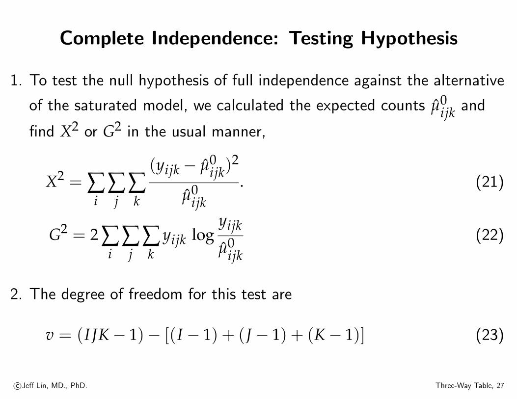
Complete Independence: Testing Hypothesis
1. To test the null hypothesis of full independence against the alternative
of the saturated model, we calculated the expected counts µ0ijk and
find X2 or G2 in the usual manner,
X2 = ∑i
∑j
∑k
(yijk − µ0ijk)
2
µ0ijk
. (21)
G2 = 2 ∑i
∑j
∑k
yijk logyijk
µ0ijk
(22)
2. The degree of freedom for this test are
v = (I JK − 1)− [(I − 1) + (J − 1) + (K − 1)] (23)
c©Jeff Lin, MD., PhD. Three-Way Table, 27
Complete Independence: Testing Hypothesis
3. In the graph, the lack of connections between the variables indicates
no relationship exist among A, B, and C.
4. This model is expressed as (A, B, C).
5. In terms of odds ratio, the model (A, B, C) implies that if we look at
the marginal table A× B, B× C, and A× C, that all of the odds
ratios in these marginal table are equal to 1.
c©Jeff Lin, MD., PhD. Three-Way Table, 28

Types of Independence: Joint Independence
c©Jeff Lin, MD., PhD. Three-Way Table, 29

Joint Independence
1. Variable C is joint independent of A and B when
πijk = πij+π++k (24)
2. This model indicates linking A and B indicates that A and B are
possible related, but not necessary so.
3. Therefore, the model of complete independence is a special case of
this one. This model is denoted as (AB, C).
c©Jeff Lin, MD., PhD. Three-Way Table, 30
Joint Independence
1. If the model of complete independence (A, B, C) fits a data set, then
the model (AB, C) will also fit, as will (AC, B) and (BC, A). In that
case, we ill prefer to use (A, B, C) because it is more parsimonious.
2. Our goal is to find the simplest model that fit the data.
c©Jeff Lin, MD., PhD. Three-Way Table, 31

Joint Independence: Point Estimation
1. Under, (AB, C),
πijk = P(A = i, B = j)P(C = k) = (αβ)ijγk (25)
where ∑i ∑j (αβ)ij = 1 and ∑k γk = 1.
2. The number of free parameters is (I J − 1) + (K − 1), and their MLestimates are
(αβ)ijyij+
n, γk =
y++kn
, for i, j, and k. (26)
3. The estimated expected frequencies are
µijk =yij+ y++k
n, for i, j, and k. (27)
c©Jeff Lin, MD., PhD. Three-Way Table, 32

Joint Independence: Point Estimation
1. Notice the similarity between this formula and the one for the model
if independence in a two-way table,
µij =yi+ y+j
n(28)
2. This is ordinary two-way independence for C and a new variable
composed of the I J combinations of levels of A and B.
3. If we view A and B as a single categorical variable with I J levels, the
goodness-of-fit test for (AB, C) is equivalent to the test of
independence between the combined variable (AB) and C.
c©Jeff Lin, MD., PhD. Three-Way Table, 33

Types of Independence: Conditional Independence
1. This model indicates that A and B may be related; A and C may be
related, and that B and C may be related, but only through their
mutual associations with A.
2. In other words, any relationship between B and C can be “full
explained” by A. This model is denoted as (AB, AC). So
πjk | i = πj+ | iπ+k | i, for all J and K. (29)
c©Jeff Lin, MD., PhD. Three-Way Table, 34

Conditional Independence: Simpson’s Paradox
1. In terms of odds ratios, this model implies that if we looks at the
B× C tables at each level of A = 1, . . . , I that the odds ratio in these
tables are not significant different from 1.
2. Notice that the odds ratios in the marginal B× C table, collapsed or
summed over A, are not necessarily 1.
3. The conditional BC odds ratios at the levels of A = 1, . . . , I can be
quite different from the marginal odds ratio.
4. In extreme cases, the marginal relationship between B and C can be
in opposite direction from their conditional relationship given A; this
is known as Simpson’s paradox.
c©Jeff Lin, MD., PhD. Three-Way Table, 35

Conditional Independence: Point Estimation
Under the conditional independence model, the probabilities can be
written as
πijk = P(A = i)P(B = j, C = k | A = i) (30)
= P(A = i)P(B = j | A = i)P(C = k | A = i) (31)
=πij+πi+k
πi++, for all i, jk (32)
= αiβ j(i)γk(i) (33)
where ∑i αi = 1, ∑j β j(i) = 1 and ∑k γk(i) = 1 for each i. The number
of free parameters is
(I − 1) + I(J − 1) + I(K − 1). (34)
c©Jeff Lin, MD., PhD. Three-Way Table, 36

Conditional Independence: Point Estimation
1. The ML estimates of these parameters are
αi = yi++/n, β j(i) = yij+/yi++, γk(i) = yi+k/yi++; (35)
for all i, j, and k.
2. The estimated expected frequencies are
µijk =yij+yi+k
yi++(36)
c©Jeff Lin, MD., PhD. Three-Way Table, 37

Conditional Independence: Point Estimation
1. Notice, again the similarity to the formula for independence in a
two-way table.
2. The test for conditional independence of B and C given A is
equivalent to separating the table by levels of A = 1, . . . , I and
testing for independence within each level.
3. The overall X2 and G2 statistics are found by summing the individual
test statistics for BC independence given A.
4. The total degrees of freedom for this test must be I(J − 1)(K − 1).
c©Jeff Lin, MD., PhD. Three-Way Table, 38

Types of Independence: Saturated (Full) Model
1. The saturated (full) model is (ABC).
2. This model allows th BC odds ratio at each level of A + 1, . . . , I to be
arbitrary.
c©Jeff Lin, MD., PhD. Three-Way Table, 39
Types of Independence: Homogeneous Association
c©Jeff Lin, MD., PhD. Three-Way Table, 40

Homogeneous Association
1. There is a model that is “intermediate” in complexity between
(AB, AC) and (ABC). Recall that (AB, AC) requires the (BC) odds
ratio at each level of A = 1, . . . .I to be equal to one.
2. Suppose that we require the BC odds ratios at each level of A to be
identical, but not necessary one.
3. This model is called homogeneous association.
4. The notation for homogeneous association model is (AB, BC, AC).
c©Jeff Lin, MD., PhD. Three-Way Table, 41

Homogeneous Association
1. The model of homogeneous association says that the conditional
relationship between any pair of variables given the third one is the
same at each level of the third one.
2. That is, there are no interactions.
3. An interaction means that the relationship between two variables
changes across the levels of a third.
c©Jeff Lin, MD., PhD. Three-Way Table, 42

Homogeneous Association
4. This is similar in spirit to the multivariate normal distribution for
continuous variables, which says that the conditional correlation
between any two variables given a third is the same for all values of
the third.
5. Under the model of homogeneous association, there are no close-form
estimate for the cell probabilities.
c©Jeff Lin, MD., PhD. Three-Way Table, 43

Homogeneous Association: Point Emstimation
ML estimates must be computed by an iterative procedure. The most
popular methods are
1. Iterative Proportional Fitting (IPF),
2. Newton-Raphson (NR).
c©Jeff Lin, MD., PhD. Three-Way Table, 44
Marginal versus Conditional Independence
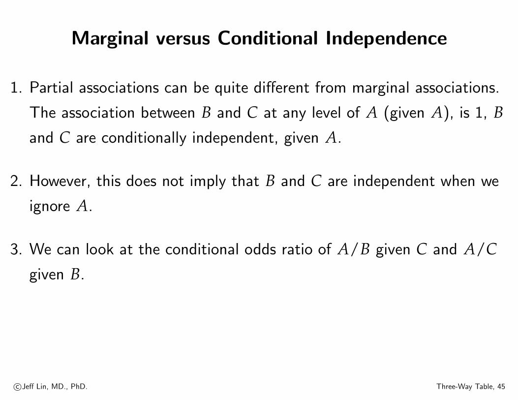
1. Partial associations can be quite different from marginal associations.
The association between B and C at any level of A (given A), is 1, Band C are conditionally independent, given A.
2. However, this does not imply that B and C are independent when we
ignore A.
3. We can look at the conditional odds ratio of A/B given C and A/Cgiven B.
c©Jeff Lin, MD., PhD. Three-Way Table, 45

Marginal versus Conditional Independence
1. Conditional independence and marginal independence both hold when
one of the stronger types of independence studied in the previous
subsections.
2. Suppose C is jointly independent of A and B, that is
πijk = πij+π++k. (37)
3. We have seen that this implies conditional independence of A and C.
c©Jeff Lin, MD., PhD. Three-Way Table, 46
Marginal versus Conditional Independence
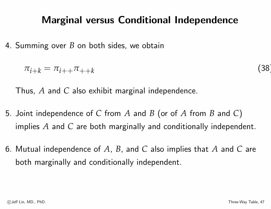
4. Summing over B on both sides, we obtain
πi+k = πi++π++k (38)
Thus, A and C also exhibit marginal independence.
5. Joint independence of C from A and B (or of A from B and C)
implies A and C are both marginally and conditionally independent.
6. Mutual independence of A, B, and C also implies that A and C are
both marginally and conditionally independent.
c©Jeff Lin, MD., PhD. Three-Way Table, 47
Marginal versus Conditional Independence
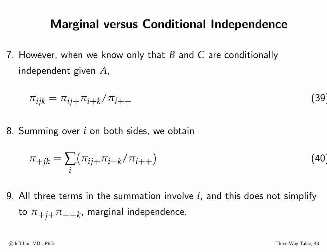
7. However, when we know only that B and C are conditionally
independent given A,
πijk = πij+πi+k/πi++ (39)
8. Summing over i on both sides, we obtain
π+jk = ∑i
(πij+πi+k/πi++
)(40)
9. All three terms in the summation involve i, and this does not simplify
to π+j+π++k, marginal independence.
c©Jeff Lin, MD., PhD. Three-Way Table, 48

Three-Way Table: Modeling Strategy
c©Jeff Lin, MD., PhD. Three-Way Table, 49
Modeling Strategy
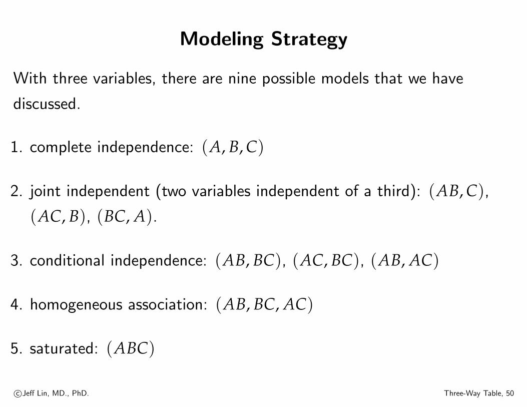
With three variables, there are nine possible models that we have
discussed.
1. complete independence: (A, B, C)
2. joint independent (two variables independent of a third): (AB, C),(AC, B), (BC, A).
3. conditional independence: (AB, BC), (AC, BC), (AB, AC)
4. homogeneous association: (AB, BC, AC)
5. saturated: (ABC)
c©Jeff Lin, MD., PhD. Three-Way Table, 50
Modeling Strategy
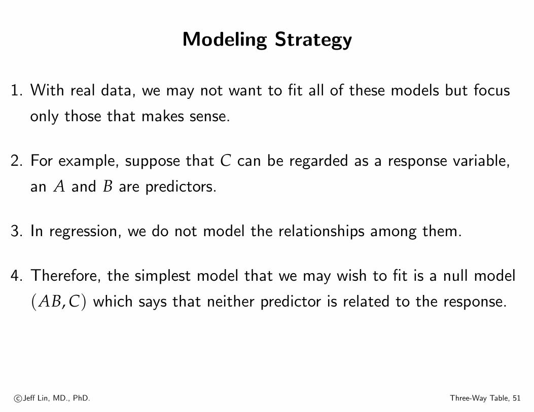
1. With real data, we may not want to fit all of these models but focus
only those that makes sense.
2. For example, suppose that C can be regarded as a response variable,
an A and B are predictors.
3. In regression, we do not model the relationships among them.
4. Therefore, the simplest model that we may wish to fit is a null model
(AB, C) which says that neither predictor is related to the response.
c©Jeff Lin, MD., PhD. Three-Way Table, 51

Modeling Strategy
1. If the null model does not fit, the we should try (AB, AC), which says
that A is related to C. but B is not.
2. This equivalent to a logistic regression for C with a main effect for Abut no effect for B.
3. We may also try (AB, BC), which is equivalent to a logistic regression
for C with main effect for B but no effect for A.
c©Jeff Lin, MD., PhD. Three-Way Table, 52

Modeling Strategy
1. If neither of those models fit, we may try the model of homogeneous
association (AB, BC, AC), which is equivalent to a logistic regression
for C within main effects for A and for B but no interaction.
2. The saturated model (ABC) is equivalent to a logistic regression for
C with a main effect for A, as a main effect for B and AB interaction.
c©Jeff Lin, MD., PhD. Three-Way Table, 53

Partitioning Chi-Squared Tests
c©Jeff Lin, MD., PhD. Three-Way Table, 54
Partitioning Chi-Squared Tests
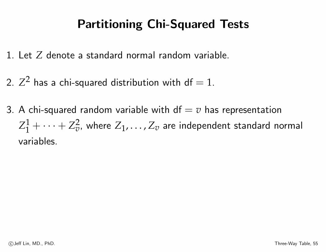
1. Let Z denote a standard normal random variable.
2. Z2 has a chi-squared distribution with df = 1.
3. A chi-squared random variable with df = v has representation
Z11 + · · ·+ Z2
v, where Z1, . . . , Zv are independent standard normal
variables.
c©Jeff Lin, MD., PhD. Three-Way Table, 55

Partitioning Chi-Squared Tests
4. A chi-squared statistic having df = v has partitionings into
independent chi-squared components—for example, into vcomponents each having df = 1
5. Conversely, if X21 and X2
2 are independent chi-squared random
variables having degrees of freedom v1 and v2, then X2 = X21 + X2
2has a chi-squared distribution with df = v1 + v2.
c©Jeff Lin, MD., PhD. Three-Way Table, 56

Partitioning Chi-Squared Tests
1. Another supplement to a chi-squared test partitions its test statistic
so that the components represent certain aspects of the effects.
2. A partitioning may show that an association reflects primary
differences between certain categories or groupings of categories.
c©Jeff Lin, MD., PhD. Three-Way Table, 57

Partitioning Chi-Squared Tests
1. We begin with a partitioning for the test of independence in a 2× Jtables.
2. We partition G2, which has df = (J − 1), into J − 1 components.
3. The jth component is G2 for a 2× 2 table where the first column
combines columns 1
4. through j of the full table and the second column is column j + 1.
c©Jeff Lin, MD., PhD. Three-Way Table, 58

Partitioning Chi-Squared Tests
5. That is, G2 for testing independence in a 2× J table equals a statistic
that compares the first two columns, plus a statistic that combines
the first two columns and compares them to the third column, and so
on, up to a statistic that combines the first J − 1 columns and
compares them to the last column.
6. Each component statistic has df = 1.
c©Jeff Lin, MD., PhD. Three-Way Table, 59
Partitioning Chi-Squared Tests
1. It might seem more natural to compute G2 for the (j− 1) separate
2× 2 tables that pair each column with a particular one, say the last.
2. However, these component statistics are not independent and do not
sum G2 for the full table.
c©Jeff Lin, MD., PhD. Three-Way Table, 60
Partitioning Chi-Squared Tests: Lancaster (1949)
1. For an I × J table, independent chi-squared components result from
comparing column 1 and 2 and then combing them and comparing
them to column 3, and so on.
2. Each of the J − 1 statistics has df = I − 1.
3. More refined partitions contain (I − 1)(J − 1) statistics, each having
df = 1.
4. One such partitioning (Lancaster 1949) applies to the (I − 1)(J − 1)separate 2× 2 tables is in Table 2.
c©Jeff Lin, MD., PhD. Three-Way Table, 61
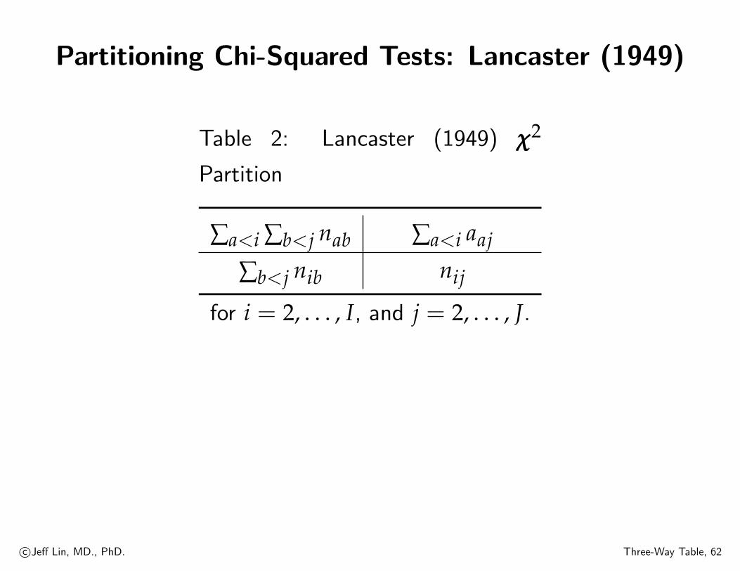
Partitioning Chi-Squared Tests: Lancaster (1949)
Table 2: Lancaster (1949) χχχ2
Partition
∑a<i ∑b<j nab ∑a<i aaj
∑b<j nib nij
for i = 2, . . . , I, and j = 2, . . . , J.
c©Jeff Lin, MD., PhD. Three-Way Table, 62

Partitioning Chi-Squared Tests
Goodman (1968, 1969a, 1971b) and Lancaster (1949, 1969) gave rules
for determining independent components of chi-squared. For forming
subtables, aiming the necessary conditions are the following:
1. The df for the subtables must sum to df for the full table.
2. Each cell count in the full table must be a cell count in one and only
one subtable.
3. Each marginal total of the full table must be a marginal total for one
and only one subtable.
c©Jeff Lin, MD., PhD. Three-Way Table, 63
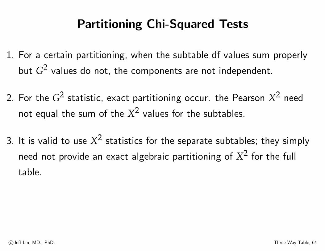
Partitioning Chi-Squared Tests
1. For a certain partitioning, when the subtable df values sum properly
but G2 values do not, the components are not independent.
2. For the G2 statistic, exact partitioning occur. the Pearson X2 need
not equal the sum of the X2 values for the subtables.
3. It is valid to use X2 statistics for the separate subtables; they simply
need not provide an exact algebraic partitioning of X2 for the full
table.
c©Jeff Lin, MD., PhD. Three-Way Table, 64
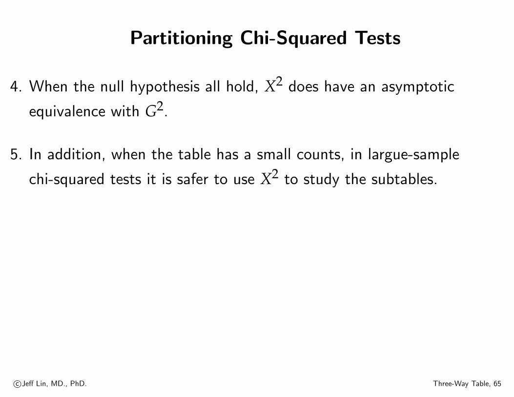
Partitioning Chi-Squared Tests
4. When the null hypothesis all hold, X2 does have an asymptotic
equivalence with G2.
5. In addition, when the table has a small counts, in largue-sample
chi-squared tests it is safer to use X2 to study the subtables.
c©Jeff Lin, MD., PhD. Three-Way Table, 65

Limitations of Chi-Squared Tests
1. Chi-squared tests of independence merely indicate the degree of
evidence of association.
2. They are rarely adequate for answering all questions about a data set.
Rather then relying solely on the results of the tests, investigate the
mature of the association:
3. Study residuals, decomposed chi-squared into components, and
estimate parameters such as odds ratios that describe the strength of
association.
c©Jeff Lin, MD., PhD. Three-Way Table, 66

Limitations of Chi-Squared Tests
4. The chi-squared tests also have limitations in the types of data to
which they apply.
5. For instance, they require large samples.
6. Also, the µij = ni+n+j/n used in X2 and G2 depend on he marginal
totals but not on the order of listing the rows and columns.
7. Thus, X2 and G2 do not change value with arbitrary re-orderings of
rows or of columns.
c©Jeff Lin, MD., PhD. Three-Way Table, 67
Limitations of Chi-Squared Tests
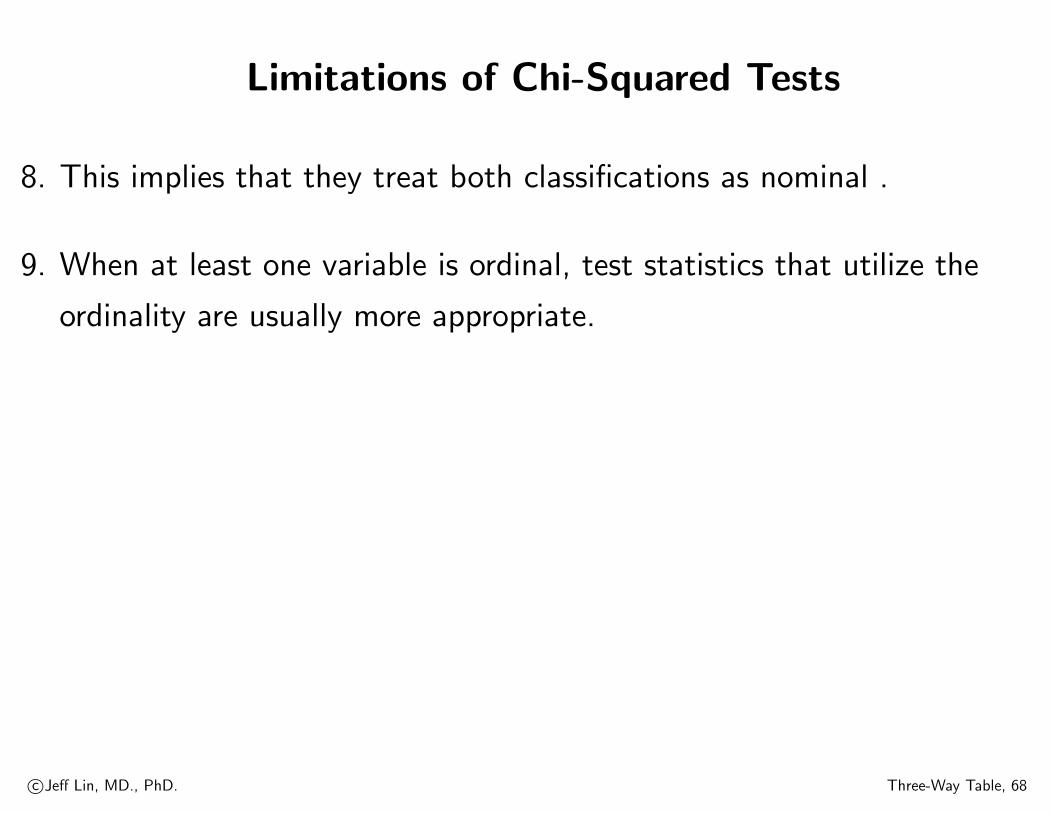
8. This implies that they treat both classifications as nominal .
9. When at least one variable is ordinal, test statistics that utilize the
ordinality are usually more appropriate.
c©Jeff Lin, MD., PhD. Three-Way Table, 68
Why Consider Independence?
c©Jeff Lin, MD., PhD. Three-Way Table, 69
Why Consider Independence?
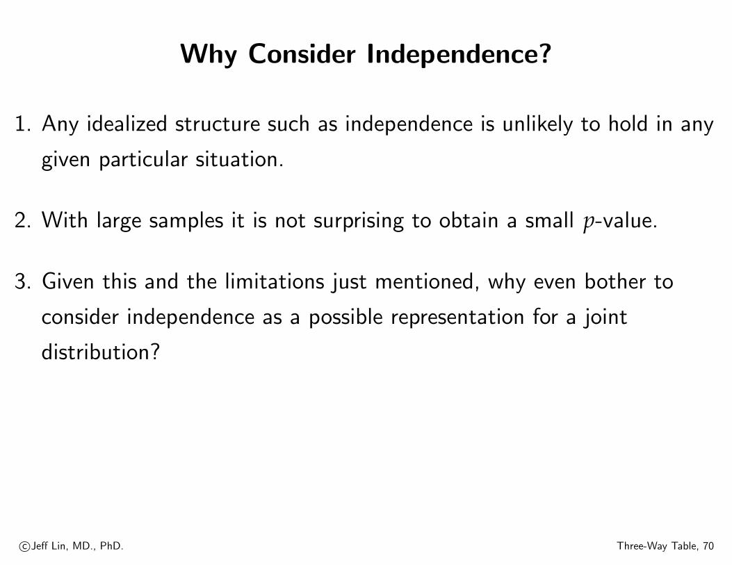
1. Any idealized structure such as independence is unlikely to hold in any
given particular situation.
2. With large samples it is not surprising to obtain a small p-value.
3. Given this and the limitations just mentioned, why even bother to
consider independence as a possible representation for a joint
distribution?
c©Jeff Lin, MD., PhD. Three-Way Table, 70

Why Consider Independence?
1. One reason refers to the benefits of model parsimony.
2. If the independence model approximates the true probabilities well,
then unless n is very large, the model-based estimates
πij = ni+n+j/n of cell probability tend to be better than the sample
proportions pij = nij/n.
3. The independence ML estimates smooth the sample counts,
somewhat damping the random sampling fluctuations.
c©Jeff Lin, MD., PhD. Three-Way Table, 71

Why Consider Independence?
4. The mean-squared error (MSE) formula
MSE = variance + (bias)2
explains why the independence estimators can have smaller MSE.
5. Although they may be biased, they have smaller variance because they
are based on estimating fewer parameters πi and π+j instead of πij.
6. Hence, MSE can be smaller unless n is so large that the bias term
dominates the variance.
c©Jeff Lin, MD., PhD. Three-Way Table, 72
Stratified Categorical Data:
The (Cochran) Mantel-Haenszel Test
c©Jeff Lin, MD., PhD. Three-Way Table, 73

Example: Coronary Artery Disease
Table 3 are based on a study on coronary artery disease (Koch, Imrery et
al. 1985). The sample is one of convenience since the patients studied
were people who came to clinic and requested an evaluation.
c©Jeff Lin, MD., PhD. Three-Way Table, 74

Example: Coronary Artery Disease
Table 3: Retrospective study: gender, ECG and disease
Disease No Disease
Gender ECG Condition (Cases) (Controls) Total
Female > 0.1 ST depression 8 10 18
Female ≤ 0.1 ST depression 4 11 15
Male > 0.1 ST depression 21 6 27
Male ≤ 0.1 ST depression 9 9 18
Total 42 36 78
c©Jeff Lin, MD., PhD. Three-Way Table, 75

Example: Coronary Artery Disease: ECG vs. Gender
Table 4: Retrospective study: EKG and Gender
Gender
ECG Condition Female Male Total
> 0.1 ST depression 18 27 45
≤ 0.1 ST depression 15 18 33
Total 33 45 78
c©Jeff Lin, MD., PhD. Three-Way Table, 76

Example: ECG and Gender
> # EKG vs. Gender
> EKG.Gender<-matrix(c(18,27,15,18),nrow=2,byrow=T)
> fisher.test(EKG.Gender)
Fisher’s Exact Test for Count Data
data: EKG.Gender
p-value = 0.6502
alternative hypothesis: true odds ratio is not equal to 1
95 percent confidence interval:
0.2932842 2.1906132
sample estimates:
odds ratio
0.8023104
c©Jeff Lin, MD., PhD. Three-Way Table, 77

Example: ECG Condition and Coronary Artery Disease
Investigators were interested in whether (electrocardiogram) ECG
measurement was associated with disease status.
Table 5: Retrospective study: ECG and coronary heart
disease
Coronary Artery Disease
ECG Condition Yes (cases) No (controls) Total
> 0.1 ST depression 29 16 45
≤ 0.1 ST depression 13 20 33
Total 42 36 78
c©Jeff Lin, MD., PhD. Three-Way Table, 78

Example: ECG and Coronary Artery Disease
> EKG.CAD<-matrix(c(29,16,13,20),nrow=2,byrow=T)
> fisher.test(EKG.CAD)
Fisher’s Exact Test for Count Data
data: EKG.CAD
p-value = 0.03894
alternative hypothesis: true odds ratio is not equal to 1
95 percent confidence interval:
1.003021 7.828855
sample estimates:
odds ratio
2.750314
c©Jeff Lin, MD., PhD. Three-Way Table, 79

Example: Gender and Coronary Artery Disease
Investigators were interested in whether gender was associated with
disease status.
Table 6: Retrospective study: gender and
Coronary Heart Disease
Coronary Artery Disease
Gender Yes (cases) No (controls) Total
Female 12 21 33
Male 30 15 45
Total 42 36 78
c©Jeff Lin, MD., PhD. Three-Way Table, 80

Example: Gender and Coronary Artery Disease
> gender.CAD<-matrix(c(12,21,30,15),nrow=2,byrow=T)
> fisher.test(gender.CAD)
Fisher’s Exact Test for Count Data
data: gender.CAD
p-value = 0.01142
alternative hypothesis: true odds ratio is not equal to 1
95 percent confidence interval:
0.09986503 0.80674974
sample estimates:
odds ratio
0.290676
c©Jeff Lin, MD., PhD. Three-Way Table, 81

Example: Coronary Artery Disease: Stratification
Gender was though to be associated with disease status, so investigators
stratified the data into female and male groups.
c©Jeff Lin, MD., PhD. Three-Way Table, 82

Example: Coronary Artery Disease: Female
Table 7: Retrospective study: ECG and Coronary Heart
Disease for Female
Female Coronary Artery Disease
ECG Condition Yes (cases) No (controls) Total
> 0.1 ST depression 8 10 18
≤ 0.1 ST depression 4 11 15
Total 12 21 33
c©Jeff Lin, MD., PhD. Three-Way Table, 83

Example: Female and Coronary Artery Disease
> Female.CAD<-matrix(c(8,10,4,11),nrow=2,byrow=T)
> fisher.test(Female.CAD)
Fisher’s Exact Test for Count Data
data: Female.CAD
p-value = 0.4688
alternative hypothesis: true odds ratio is not equal to 1
95 percent confidence interval:
0.4113675 12.9927377
sample estimates:
odds ratio
2.147678
c©Jeff Lin, MD., PhD. Three-Way Table, 84

Example: Coronary Artery Disease: Male
Table 8: Retrospective study: ECG and Coronary Heart
Disease for Male
Male Coronary Artery Disease
ECG Condition Yes (cases) No (controls) Total
> 0.1 ST depression 21 6 27
≤ 0.1 ST depression 9 9 18
Total 30 15 45
c©Jeff Lin, MD., PhD. Three-Way Table, 85
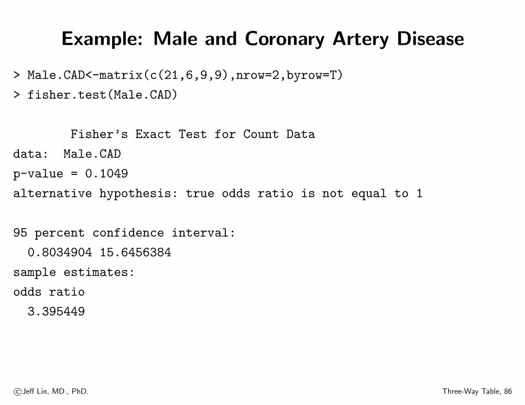
Example: Male and Coronary Artery Disease
> Male.CAD<-matrix(c(21,6,9,9),nrow=2,byrow=T)
> fisher.test(Male.CAD)
Fisher’s Exact Test for Count Data
data: Male.CAD
p-value = 0.1049
alternative hypothesis: true odds ratio is not equal to 1
95 percent confidence interval:
0.8034904 15.6456384
sample estimates:
odds ratio
3.395449
c©Jeff Lin, MD., PhD. Three-Way Table, 86
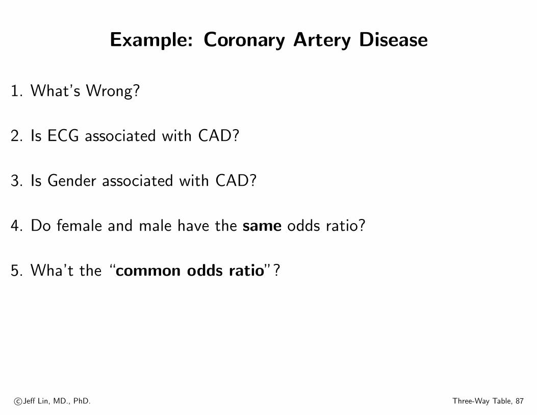
Example: Coronary Artery Disease
1. What’s Wrong?
2. Is ECG associated with CAD?
3. Is Gender associated with CAD?
4. Do female and male have the same odds ratio?
5. Wha’t the “common odds ratio”?
c©Jeff Lin, MD., PhD. Three-Way Table, 87

Stratified Categorical Data:
The (Cochran) Mantel-Haenszel Test
c©Jeff Lin, MD., PhD. Three-Way Table, 88

Confounding Variable
1. A confounding variable is a variable that is associated with both the
disease and the exposure variable.
2. Such a variable must usually be controlled for before disease-exposure
relationship.
c©Jeff Lin, MD., PhD. Three-Way Table, 89

Confounding Variables and Stratification
1. The analysis of disease-exposure relationships in separate sub-groups
of the data, where the sub-groups are defined by one or more
potential confounders, referred to as stratification.
2. The sub-groups themselves are referred to as strata.
3. In general the data will be stratified into k sub-groups according to
one or more confounding variables to make the units within a stratum
as homogeneous as possible.
4. The data for each stratum consist of a 2× 2 contingency table, as in
Table 9, relating exposure to disease.
c©Jeff Lin, MD., PhD. Three-Way Table, 90
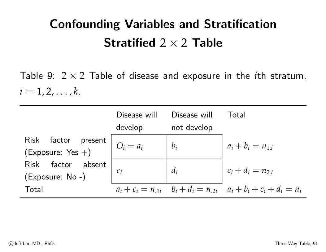
Confounding Variables and Stratification
Stratified 2× 2 Table
Table 9: 2× 2 Table of disease and exposure in the ith stratum,
i = 1, 2, . . . , k.
Disease will Disease will Total
develop not develop
Risk factor present
(Exposure: Yes +)Oi = ai bi ai + bi = n1.i
Risk factor absent
(Exposure: No -)ci di ci + di = n2.i
Total ai + ci = n.1i bi + di = n.2i ai + bi + ci + di = ni
c©Jeff Lin, MD., PhD. Three-Way Table, 91
Stratified 2× 2 Table
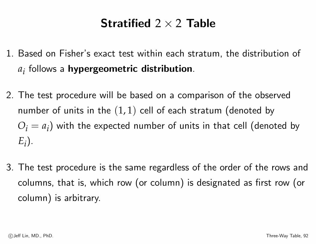
1. Based on Fisher’s exact test within each stratum, the distribution of
ai follows a hypergeometric distribution.
2. The test procedure will be based on a comparison of the observed
number of units in the (1, 1) cell of each stratum (denoted by
Oi = ai) with the expected number of units in that cell (denoted by
Ei).
3. The test procedure is the same regardless of the order of the rows and
columns, that is, which row (or column) is designated as first row (or
column) is arbitrary.
c©Jeff Lin, MD., PhD. Three-Way Table, 92

Mantel-Haenszel Test
The expected value of Oi and variance of Oi is
Ei = E(Oi) =(ai + bi)(ai + ci)
ni(41)
Vi = Var(Oi) =(ai + bi)(ci + di)(ai + ci)(bi + di)
n2i (ni − 1)
(42)
c©Jeff Lin, MD., PhD. Three-Way Table, 93

Mantel-Haenszel Test for Association
over Different Strata
Mantel-Haenszel Test is used to assess the association between a
dichotomous disease and a dichotomous exposure variable after
controlling for one or more confounding variables.
c©Jeff Lin, MD., PhD. Three-Way Table, 94

Mantel-Haenszel Test for Association
over Different Strata
Under H0, there is no association between disease and exposure, then let
O =k∑i=1
Oi =k∑i=1
ai (43)
E =k∑i=1
Ei =k∑i=1
(ai + bi)(ai + ci)ni
(44)
V =k∑i=1
Vi =k∑i=1
(ai + bi)(ci + di)(ai + ci)(bi + di)n2
i (ni − 1)(45)
X2MH =
( | O− E | − 0.5)2
Vasym∼ χχχ2
1 (46)
c©Jeff Lin, MD., PhD. Three-Way Table, 95

Mantel-Haenszel Test for Association
over Different Strata
1. Under H0 X2MH asymptotically follows chi-squared distribution with 1
degree of freedom.
2. For two-sided test with significance level α, we reject H0 if
X2MH > χχχ2
1,1−α.
3. p-value = Pr(χχχ21 ≥ X2
MH)
c©Jeff Lin, MD., PhD. Three-Way Table, 96
Interaction Effect: Confounder and Effect Modifier
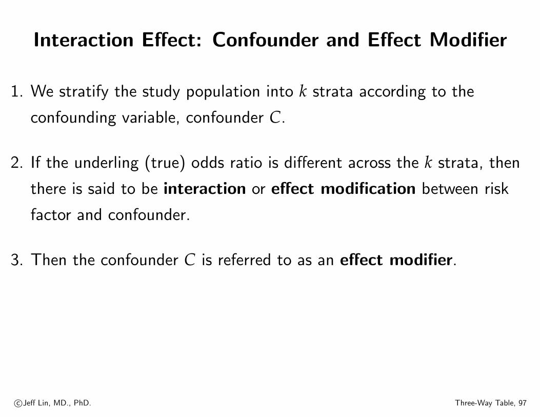
1. We stratify the study population into k strata according to the
confounding variable, confounder C.
2. If the underling (true) odds ratio is different across the k strata, then
there is said to be interaction or effect modification between risk
factor and confounder.
3. Then the confounder C is referred to as an effect modifier.
c©Jeff Lin, MD., PhD. Three-Way Table, 97

Mantel-Haenszel Test:
Chi-square Test for Homogeneity of Odds Ratios over
Different Strata (Woolf’s Method)
1. The Mantel-Haenszel test provides a test of significance of the
relationship between disease and exposure.
2. If we reject the null hypothesis in Mantel-Haenszel test, there exist
association of disease and risk factor.
c©Jeff Lin, MD., PhD. Three-Way Table, 98

Mantel-Haenszel Test:
Chi-square Test for Homogeneity of Odds Ratios over
Different Strata (Woolf’s Method)
1. Let ORi is underling odds ratio in the ith stratum.
2. To test the hypothesis
H0 : OR1 = OR2 = · · · = ORk; (47)
vs. HA : at least two of the ORi are significant different (48)
3. This is to test whether a common odds ratio (homogeneity) exist
when there is association of disease and risk factor given controlling
the confounding factor with stratification.
c©Jeff Lin, MD., PhD. Three-Way Table, 99
Mantel-Haenszel Test:
Chi-square Test for Homogeneity of Odds Ratios
over Different Strata (Woolf’s Method)
The chi-square test for homogeneity is calculated as following:
c©Jeff Lin, MD., PhD. Three-Way Table, 100
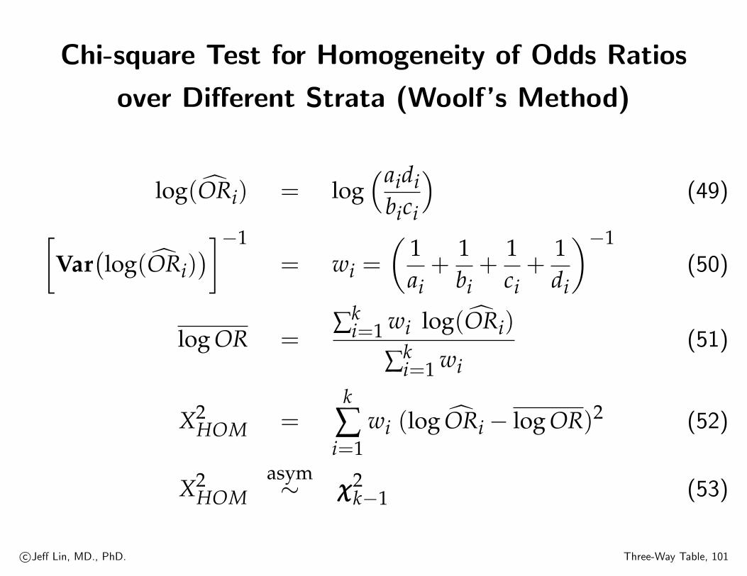
Chi-square Test for Homogeneity of Odds Ratios
over Different Strata (Woolf’s Method)
log(ORi) = log(aidi
bici
)(49)[
Var(log(ORi)
)]−1= wi =
(1ai
+1bi
+1ci
+1di
)−1(50)
log OR =∑k
i=1 wi log(ORi)
∑ki=1 wi
(51)
X2HOM =
k∑i=1
wi (log ORi − log OR)2 (52)
X2HOM
asym∼ χχχ2
k−1 (53)
c©Jeff Lin, MD., PhD. Three-Way Table, 101

Chi-square Test for Homogeneity of Odds Ratios
over Different Strata (Breslow-Day Method in SAS)
Similar to Woolf’s method
c©Jeff Lin, MD., PhD. Three-Way Table, 102
Mantel-Haenszel Test:
Chi-square Test for Homogeneity of Odds Ratios
over Different Strata (Woolf’s Method)
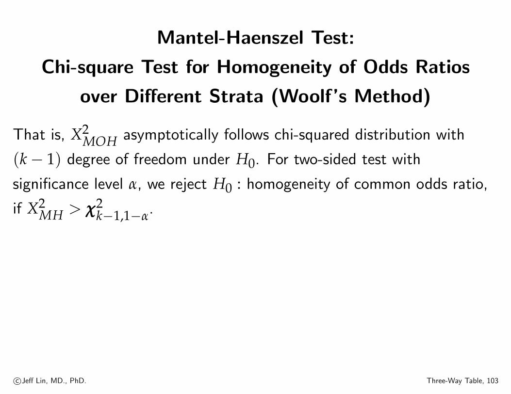
That is, X2MOH asymptotically follows chi-squared distribution with
(k− 1) degree of freedom under H0. For two-sided test with
significance level α, we reject H0 : homogeneity of common odds ratio,
if X2MH > χχχ2
k−1,1−α.
c©Jeff Lin, MD., PhD. Three-Way Table, 103
Mantel-Haenszel Estimator of
the Common Odds Ratio for Stratified Data
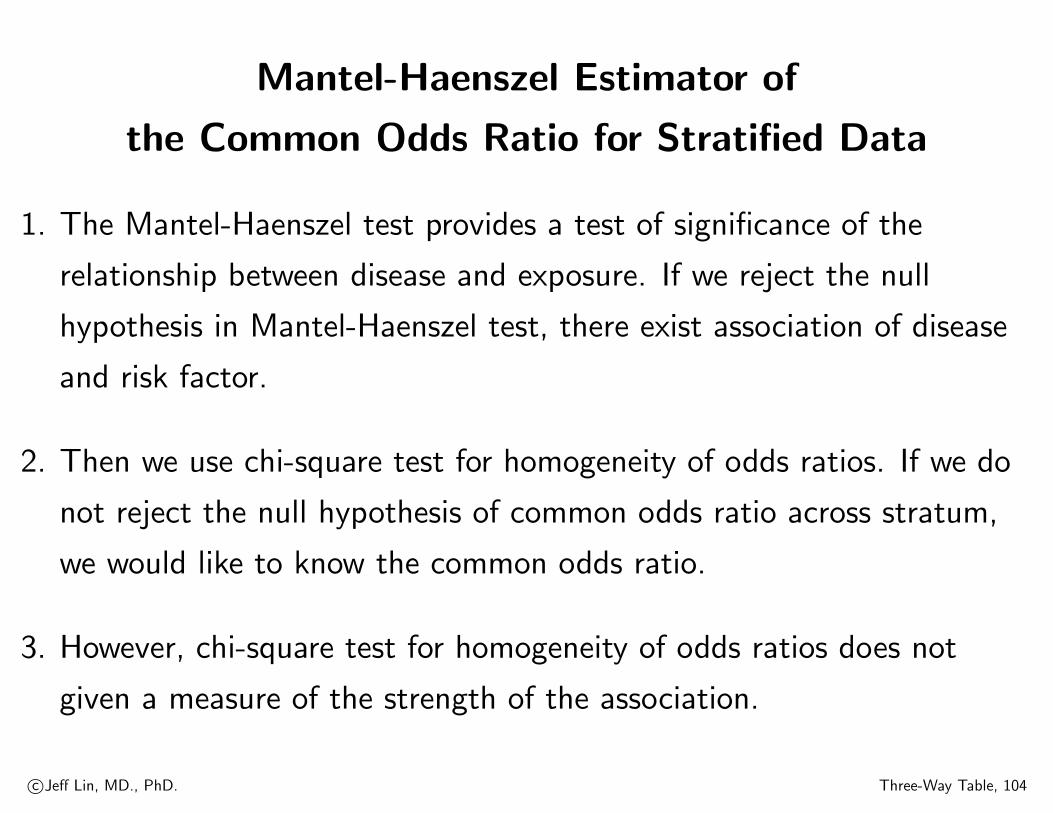
1. The Mantel-Haenszel test provides a test of significance of the
relationship between disease and exposure. If we reject the null
hypothesis in Mantel-Haenszel test, there exist association of disease
and risk factor.
2. Then we use chi-square test for homogeneity of odds ratios. If we do
not reject the null hypothesis of common odds ratio across stratum,
we would like to know the common odds ratio.
3. However, chi-square test for homogeneity of odds ratios does not
given a measure of the strength of the association.
c©Jeff Lin, MD., PhD. Three-Way Table, 104

Mantel-Haenszel Estimator of
the Common Odds Ratio for Stratified Data
In general, it is important to test for homogeneity of the stratum-specific
odds ratio. If the true odds ratios are different, then it makes no sense
to obtain a pooled-odds ratio estimate.
c©Jeff Lin, MD., PhD. Three-Way Table, 105

Mantel-Haenszel Estimator of
the Common Odds Ratio for Stratified Data
In a collection of k× 2× 2 contingency tables, where the ith table,
Table 10, corresponding to the ith stratum.
Table 10: Mantel-Haenszel Test: The ith Observed 2× 2 Table
ith Stratum Variable YVariable X level 1 level 2 Total
level 1 ai bi ai + bi = n1.ilevel 2 ci di ci + di = n2.iTotal a + c = n.1i b + d = n.2i a + b + c + d = n..i = ni
c©Jeff Lin, MD., PhD. Three-Way Table, 106

Common Odds Ratio for Stratified Data
ORMH = ∑i(aidi)/ni∑i(bici)/ni
(54)
Var(log ORMH) = ∑ πiRi2(∑i Ri)2 + ∑(πiSi + QiRi)
2(∑ Ri)(∑ Si)+ ∑ QiSi
2(∑ Si)2
(55)
where πi =ai + di
ni, Qi =
bi + cini
, (56)
Ri =ai dini
, Si =bi cini
(57)
(1− α)× 100%C.I. :
exp[
log ORMH ± Z1−α/2
√Var(log ORMH)
](58)
c©Jeff Lin, MD., PhD. Three-Way Table, 107

Mantel-Haenszel Estimator of the Common Odds
Ratio for Stratified Data
Alternatively, we can use the equation (51) as the common odds ratio
estimator.
log(ORi) = log(aidi
bici
)(59)[
Var(log(ORi)
)]−1= wi =
(1ai
+1bi
+1ci
+1di
)−1(60)
log OR =∑k
i=1 wi log(ORi)
∑ki=1 wi
(61)
c©Jeff Lin, MD., PhD. Three-Way Table, 108

Example: Coronary Artery Disease
1. For the Table of “Gender and Disease”, Pearson’s Chi-Square Test X2
is 7.035, p-value is 0.008.
2. For female, ECG > 0.1 ST depression and Disease, X2 is 1.117,
p-value is 0.290. OR is 2.2.
3. For male: ECG > 0.1 ST depression and Disease, X2 is 3.750, p-value
is 0.053. OR is 3.5.
c©Jeff Lin, MD., PhD. Three-Way Table, 109

Example: Coronary Artery Disease
4. X2MH is 4.503 (1 df) and p-value is 0.034.
5. There is association between ECG and disease after controlling gender.
6. X2HOM is 0.215 (1 df) and p-value is 0.643.
7. A common odds ratio exists between ECG and disease.
8. The common odds ration, ORMH, is 2.847, and 95% C.I. is (1.083,
7.482).
c©Jeff Lin, MD., PhD. Three-Way Table, 110

Notes: Stratification
1. The fact that a marginal table (i.e. pool over gender) may exhibit an
association completed different from a partial tables (individual tables
for male and female) is known as Simpson’s Paradox (Simpson
1951).
2. We should analyze the data following the design of original study.
c©Jeff Lin, MD., PhD. Three-Way Table, 111

Example: Coronary Artery Disease
> CAD <-array(c(8, 4, 10, 11,
21, 6, 9, 9,),
dim = c(2, 2, 2),
dimnames = list(
EKG = c(">=0.1 ST Dep", "< 0.1 ST Dep"),
Response = c("Case", "Control"),
Penicillin.Level = c("Female", "Male")))
c©Jeff Lin, MD., PhD. Three-Way Table, 112
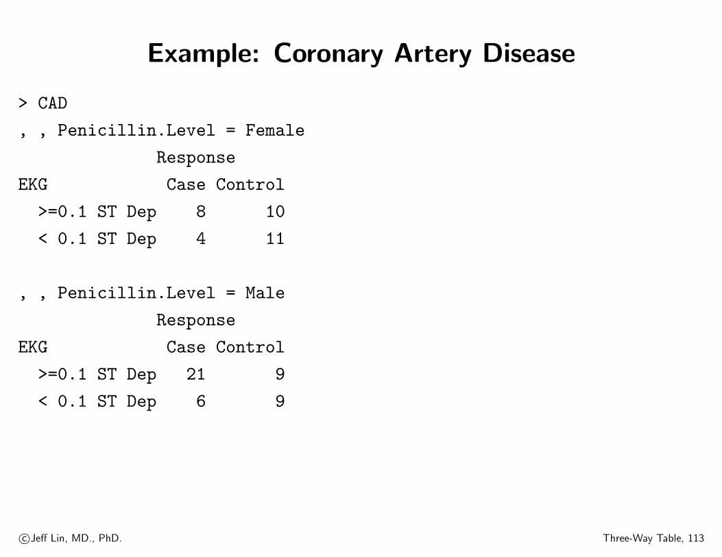
Example: Coronary Artery Disease
> CAD
, , Penicillin.Level = Female
Response
EKG Case Control
>=0.1 ST Dep 8 10
< 0.1 ST Dep 4 11
, , Penicillin.Level = Male
Response
EKG Case Control
>=0.1 ST Dep 21 9
< 0.1 ST Dep 6 9
c©Jeff Lin, MD., PhD. Three-Way Table, 113

Example: Coronary Artery Disease
> mantelhaen.test(CAD,correct=FALSE)
Mantel-Haenszel chi-squared test without continuity correction
data: CAD
Mantel-Haenszel X-squared = 4.5026, df = 1, p-value = 0.03384
alternative hypothesis: true common odds ratio is not equal to 1
95 percent confidence interval:
1.076514 7.527901
sample estimates:
common odds ratio
2.846734
c©Jeff Lin, MD., PhD. Three-Way Table, 114

Example: Coronary Artery Disease
> mantelhaen.test(CAD)
Mantel-Haenszel chi-squared test with continuity correction
data: CAD
Mantel-Haenszel X-squared = 3.5485, df = 1, p-value = 0.0596
alternative hypothesis: true common odds ratio is not equal to 1
95 percent confidence interval:
1.076514 7.527901
sample estimates:
common odds ratio
2.846734
c©Jeff Lin, MD., PhD. Three-Way Table, 115
Example: Coronary Artery Disease
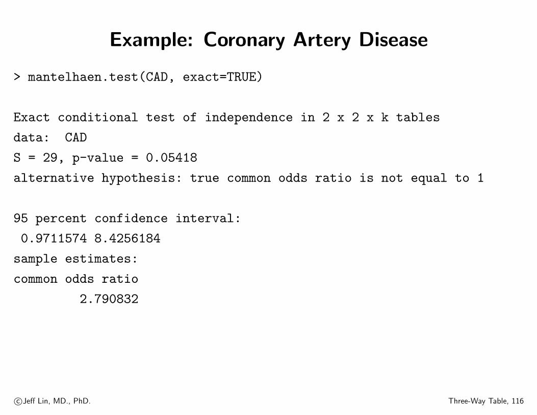
> mantelhaen.test(CAD, exact=TRUE)
Exact conditional test of independence in 2 x 2 x k tables
data: CAD
S = 29, p-value = 0.05418
alternative hypothesis: true common odds ratio is not equal to 1
95 percent confidence interval:
0.9711574 8.4256184
sample estimates:
common odds ratio
2.790832
c©Jeff Lin, MD., PhD. Three-Way Table, 116

Example: Coronary Artery Disease
> woolf <- function(x) {
x <- x + 1 / 2
k <- dim(x)[3]
or <- apply(x, 3,
function(x)(x[1,1]*x[2,2])/(x[1,2]*x[2,1]))
w <- apply(x, 3,
function(x) 1 / sum(1 / x))
1 - pchisq(sum(w * (log(or)
- weighted.mean(log(or), w)) ^ 2), k - 1)
}
c©Jeff Lin, MD., PhD. Three-Way Table, 117

Example: Coronary Artery Disease
> woolf(CAD)
[1] 0.6270651 # p-value
c©Jeff Lin, MD., PhD. Three-Way Table, 118
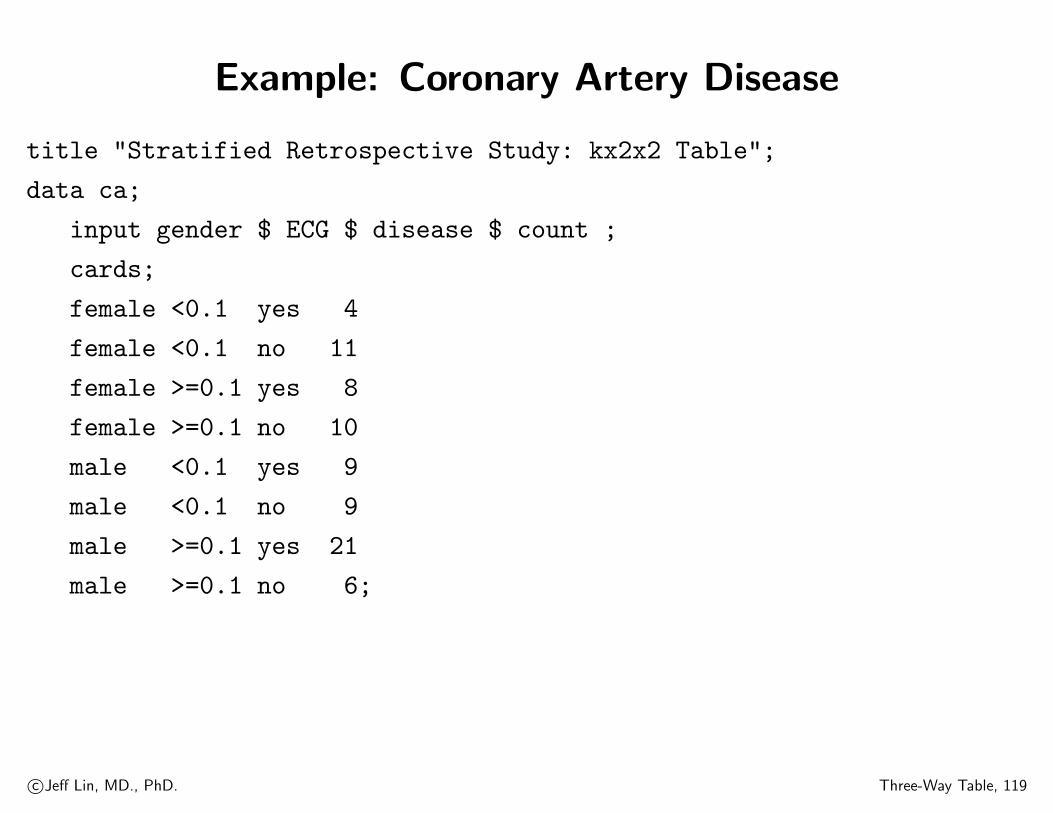
Example: Coronary Artery Disease
title "Stratified Retrospective Study: kx2x2 Table";
data ca;
input gender $ ECG $ disease $ count ;
cards;
female <0.1 yes 4
female <0.1 no 11
female >=0.1 yes 8
female >=0.1 no 10
male <0.1 yes 9
male <0.1 no 9
male >=0.1 yes 21
male >=0.1 no 6;
c©Jeff Lin, MD., PhD. Three-Way Table, 119

Example: Coronary Artery Disease
proc freq;
weight count;
tables gender*disease / nocol nopct chisq relrisk ;
tables gender*ECG*disease / nocol nopct cmh chisq relrisk;
tables ecg*disease / exact relrisk ;
run;
c©Jeff Lin, MD., PhD. Three-Way Table, 120

Example: Coronary Artery Disease
Table of gender by disease
gender disease
Frequency|
Row Pct |no |yes | Total
---------+--------+--------+
female | 21 | 12 | 33
| 63.64 | 36.36 |
---------+--------+--------+
male | 15 | 30 | 45
| 33.33 | 66.67 |
---------+--------+--------+
Total 36 42 78
c©Jeff Lin, MD., PhD. Three-Way Table, 121

Example: Coronary Artery Disease
Statistics for Table of gender by disease
Statistic DF Value Prob
-------------------------------------------------------
Chi-Square 1 7.0346 0.0080
Likelihood Ratio Chi-Square 1 7.1209 0.0076
Continuity Adj. Chi-Square 1 5.8681 0.0154
Fisher’s Exact Test
----------------------------------
Two-sided Pr <= P 0.0114
Estimates of the Relative Risk (Row1/Row2)
Type of Study Value 95% Confidence Limits
--------------------------------------------------------
Case-Control (Odds Ratio) 3.5000 1.3646 8.9771
c©Jeff Lin, MD., PhD. Three-Way Table, 122

Example: Coronary Artery Disease
Controlling for gender=female
ECG disease
Frequency|
Row Pct |no |yes | Total
---------+--------+--------+
<0.1 | 11 | 4 | 15
| 73.33 | 26.67 |
---------+--------+--------+
>=0.1 | 10 | 8 | 18
| 55.56 | 44.44 |
---------+--------+--------+
Total 21 12 33
c©Jeff Lin, MD., PhD. Three-Way Table, 123

Example: Coronary Artery Disease
Controlling for gender=female
Statistic DF Value Prob
------------------------------------------------------
Chi-Square 1 1.1175 0.2905
Fisher’s Exact Test
----------------------------------
Two-sided Pr <= P 0.4688
Type of Study Value 95% Confidence Limits
-------------------------------------------------------
Case-Control (Odds Ratio) 2.2000 0.5036 9.6107
c©Jeff Lin, MD., PhD. Three-Way Table, 124

Example: Coronary Artery Disease
Controlling for gender=male
ECG disease
fREQUENCY|
Row Pct |no |yes | Total
---------+--------+--------+
<0.1 | 9 | 9 | 18
| 50.00 | 50.00 |
---------+--------+--------+
>=0.1 | 6 | 21 | 27
| 22.22 | 77.78 |
---------+--------+--------+
Total 15 30 45
c©Jeff Lin, MD., PhD. Three-Way Table, 125

Example: Coronary Artery Disease
Controlling for gender=male
Statistic DF Value Prob
------------------------------------------------------
Chi-Square 1 3.7500 0.0528
Fisher’s Exact Test
----------------------------------
Two-sided Pr <= P 0.1049
Type of Study Value 95% Confidence Limits
-------------------------------------------------------
Case-Control (Odds Ratio) 3.5000 0.9587 12.7775
c©Jeff Lin, MD., PhD. Three-Way Table, 126

Example: Coronary Artery Disease
Cochran-Mantel-Haenszel Statistics (Based on Table Scores)
Statistic Alternative Hypothesis DF Value Prob
---------------------------------------------------------
3 General Association 1 4.5026 0.0338
c©Jeff Lin, MD., PhD. Three-Way Table, 127

Example: Coronary Artery Disease
Type of Study Method Value 95% Confidence Limits
-----------------------------------------------------------
Case-Control Mantel-Haenszel 2.8467 1.0765 7.5279
c©Jeff Lin, MD., PhD. Three-Way Table, 128

Example: Coronary Artery Disease
Breslow-Day Test for
Homogeneity of the Odds Ratios
------------------------------
Chi-Square 0.2155
DF 1
Pr > ChiSq 0.6425
Total Sample Size = 78
c©Jeff Lin, MD., PhD. Three-Way Table, 129