Ann. Inst. Statist. Math. Vol. 40, No. 1, 149-163 (1988)

TESTS FOR THE MARGINAL PROBABILITIES IN THE TWO- WAY CONTINGENCY TABLE UNDER RESTRICTED

ALTERNATIVES

KAZUO ANRAKU 1, AKIHIRO NISHI 2 AND TAKASHI YANAGAWA 3

IT he Institute of Statistical Mathematics, 4-6-7 Minami-Azabu, Minato-ku, Tokyo 106, Japan 2Faculty of Education, Saga University, Saga 840, Japan

3 Department of Mathematics, Kyushu University 33, Fukuoka 812, Japan

(Received February 26, 1986; revised April 27, 1987)

Abstract. Testing hypotheses on the marginal probabilities of a two-way contingency table is discussed. Three statistics are considered for testing the hypothesis of specified probabilities in the margins against alternatives with certain kind of order restriction. The properties of these statistics are discussed and their asymptotic behaviors are compared in depth. An application which motivated the consideration of the original testing problem is illustrated with a practical data.

Key words and phrases: Asymptotic power, categorical data, restricted alternative, most stringent somewhere most powerful test.

1. Introduction

Denote by pab the (a, b)-cell probability of a ( r + l ) × ( c + 1) contingency table. Put

pa. = ~ pab

where

p.b=Zpab, a = 1,..., r + 1; b = l , . . . , c + 1 , a

Ea ~ p a b = Z p a . = ~ p . b = l . a

The purpose of this paper is to consider testing problem of the hypothesis,

H : p a . = p ° . , p .b=pob, a = 1, . . . , r ; b = 1 .... , c ,

against

149

150 K A Z U O A N R A K U E T A L .

l t ~ m K'aZ:lpa.<aZp~. p.b<bZP.°b 1 = 1,..., r; m: l , . . . , c

= ' b= l - - '

with at least one inequality strict, wherep °. and p.°b, a= 1,..., r; b - 1,..., c, are given constants.

l l

Testing the hypothesispa.= pO. for all a against a__E1 pa._<a=E ~ p°a., 1----- 1,..., r,

that is the hypotheses regarding one of the two margins of a contingency table, has been considered by Schaafsma (1966). The problem in this paper is concerned with the two margins of a contingency table.

Three statistics are considered in Section 2 which lead to asymptotic tests for testing the hypotheses. The first statistic is constructed directly by applying the most stringent somewhere most powerful (MSSMP-) principle discussed by Schaafsma and Smid (1966) for a general class of multivariate one-sided test. On the other hand, the second and third statistics are constructed by combining two MSSMP-test statistics for the hypotheses regarding each of two margins: the first one simply adds the two statistics, but the second one uses the likelihood ratio (LR-) principle for the combination. In Section 3 we consider an example from a multiply matched case-control study. This supplies a ground for considering the above hypotheses. The approximate p-values of these three tests are obtained for the purpose of illustration by using the one-to-three matched data from a case-control study for studying the association of stomach cancer and neutritious pattern. The asymptotic efficiency of the three tests is considered in Section 4 by employing the Pitman efficiency or comparing their asymptotic powers.

2. The construction of tests

We consider first in Subsection 2.1 the MSSMP-test statistic for testing hypotheses with restricted alternatives under a general framework of multivariate normal distribution, and then introduce "approximately MSSMP-test" for H vs. K in Subsection 2.2. The T-test and R-test are introduced in Subsections 2.3 and 2.4.

2.1 Preliminary Let X=(X~,..., Xh)' be a random vector distributed as an h-variate

normal distribution with mean/~ and known covariance matrix A=(Alm). Consider testing the hypothesis

H ' : / ~ = 0 against K ' : p _ > 0 (p~O) ,

where/~>__0 means that all components of/~ are non-negative. For the purpose of constructing explicitly the statistic for testing H'

against K', we employ the MSSMP-principle. The general form of the

TESTS FOR THE MARGINAL PROBABILITIES 151

MSSMP-test given by Schaafsma and Smid (1966) is represented by; Reject H' iff<~, X>_> constant, where < . , .> is the inner product defined by <u, v>=u'A-lv for u, v e/~, and ~ is a non-negative vector which minimizes the maximum angles between 4, 4 ->0, and each axis el--(1,0,..., 0)',..., eh=(0,..., 0, 1)'.

Generally it is difficult to express the MSSMP-test statistics explicitly. However, we may show:

THEOREM 2.1. If d( v/--~,..., V/~)'>O, the MSSMP-tes t for H' against K' is expressed by

h

1= I

(2.1) Reject H' i f f ~/:lZ Z l~lm VI--~l m:lh > Ua, ,

where 2 tl is the (1, l)-element of ,4 -l and ua is the upper a-quantile o f the standard normal distribution.

PROOF. It is clear that if there exists ~_>0 which satisfies

(2.2) < ~,el > < ~,e2 > _ < ~ , e h >

I1 1111e ll II ll lie211 1141111ehll

then the 4 minimizes the maximum angles between 4 and each axis el, e2,..., eh. Thus the MSSMP-test is given by this 4. We now obtain the 4 satisfying (2.2).

Put 4"A-~=(yl,..., yh), then <4, el>=Yl, and since ffetll it follows that

4=cA(v/-2Tr,..., X / ~ ) ' for a constant c. When c>0, 4_>0 from the assumption of the theorem. Substituting this ~ to the general form we have (2.1).

Note that the vector cA(x/-~, . . . , x / r~ ) ' is a normal vector of the elliptic

quadric x 'Ax=c (>0), in R h, at the point k(x/-2rr,..., x ~ ) ' with x/k=

c / ) ? , ~ 2~/. The condition A (x /~ r, .... x/rff~)'_>0 is satisfied, for example, l , J

when all random variables X's are positively correlated, or equally correlated (also see the application below).

2.2

Put

S-test Applying the above result, we construct a statistic for testing H against K.

1

Zt = n-1/2• (np °. - Ha.) a= 1

m

Z,+m = n-l/2Z (np.°b -- n.b) , b=l

l = 1, . . . ,r ,

m = 1 , . . . , c ,

152 KAZUO ANRAKU ET AL,

Z = ( Z t , . . . , Z h ) ' , h = r + c ,

l

Or = ~ (pO. _p~ . ) l = 1 , . . , r , a = 1 ~ "

m

O~+m = ~1= (p°'b - p . b ) , m = 1,..., c ,

0 = (01 ..... Oh)' , h = r + c .

It is straightforward to show that Z - n 1/20 is asymptotically distributed as an h-variate normal distr ibution with mean 0 and covariance matr ix Z = (arm), where

~ l m = a--]=l b=~l ( p a , b - r - - p a . p . O - r )

\a=r+ 1 ] \ b=r+ 1 ]

for 1 <_l<_m<_r ,

for 1= 1 .... , r ; m = r + 1 , . . . , h ,

for r + l < _ l < m < _ h .

Since the hypotheses H a n d Kare equivalent to H": 0=0 and K": 0>0, we may use from Theorem 2.1 the following test statistic for testing H against K:

S =

h Z ~a.u Zl l= 1

~/ h h z

1=1 rn=l

when the condit ion

(2.3) _> o ,

is satisfied, where Z,=(at*) is a consistent est imator of Z under H and - r , 1 =(at, m) is the inverse of S . . We call the test based on S the S-test. The test is an approximate ly MSSMP-tes t . It follows that the S-test is asymptotically the uniformly most powerful test for the alternatives in the direction specified

o 11 ii by 0 = 0 =cZ(X/~ol, . . . , ~ ) ' , c>0, where ao is the (i, /)-element of Z "-1.

2.3 T-test The approximately MSSMP-tes t for the corresponding hypotheses

regarding one of the margins of the contingency table has been considered by Schaafsma (1966). The test statistic is given by

= (wl'l'J2 t=l \ Ql ] Z~ ,

TESTS FOR THE M A R G I N A L PROBABILITIES 153

where

= p~.-l wlt + p~+T! , 1 = 1,..., r ,

and

r ( QI=~ p'°" r+~-I 2 ~r+l- I 2

a:l - - t=-, ,,~ p?" "

Let T2, W2m, m = 1,..., c and Q2 be corresponding ones for the other margin. We consider the following test statistic T for testing H vs. K:

T~ + T2 T= '

where

d = I Iw" l ':` [w,,i,,2 [w2,1,: [w2q,,q, ~ O t ) " ' " t O , ) '~--~2) '""~Q21 1"

T is simpler than S and has no restriction. We call the test based on T the T-test. T is asymptotically distributed as the standard normal distribution

under H. It is easily seen that S= T, when d=c(x/-~,l,... , x/-~,~) ' for some positive constant c.

It follows that the T-test is asymptotically the uniformly most powerful test for the alternatives in the direction specified by o=Ol=c,rd, c>0.

2.4 R-test Kud6 (1963) considered the LR-principle for testing hypotheses with

restricted alternatives under multivariate normal distribution. Although the test by the principle is not easily available when h>4, we may apply the principle to the asymptotic distribution of (T~, T2). Consider the statistic,

_ 2 -1/2 2 (1 p,) (T~1 + T2 - 2p , T1T2) 1/2

R = (1 p2,)-l/2(T, - p , T2) (1 p2,)-'/2(T2 - p, TI)

if TI_>0, T 2 _ 0 , if T 2 < 0 , T~>T2, if T ~ < 0 , T2>_Tt,

wherep , is a consistent estimator of p, the correlation coefficient of TI and T2;

(2.4) 1 k Z, X/~tx/-W--~(p~m-pT.p°,,,) ? - x/Q1Q2 t=-i m=l

under H. If (7"1, /'2) were distributed exactly as the bivariate normal

154 KAZUO ANRAKU ET AL.

distribution N(/£/1,//./2, 1, 1, p*), the statistic R is the LR-test statistic for the null hypothesis, H":/t~=/~2=0, against the alternative, K":/LI_>0,/~2>_0. The test rejects H iff R>_ca, where ca is the critical point at the significance level a. Following Chatterjee and De (1972) we may obtain an approximate value of ca by solving

a = { 1 - Fz~(c2)} { 1 _ (2z0-~cos-lp.} + 1 _ qb(c),

where Fx~ and • are the distr ibution functions of the central z2-distribution with 2 degrees of f reedom and the standard normal distribution.

Before compar ing the asymptotic efficiency of the tests based on statistics S, T and R we look at an application of the tests briefly in the next section.

3. An application

Several controls are matched frequently to a case in a comparat ive study by means of extraneous variables. Let Xi be a r andom sample f rom the case, Yo be a r andom sample f rom the j - th control matched to the case, j = 1,..., k, and Vi be the vector of extraneous variables used for the matching. Suppose that X~ and Y,,.. . , Y~k are conditionally independent and that Yg~,..., Y~k are identically distr ibuted when condi t ioned on Vi. Let F(xl vi) and G(yl v~) be condit ional distr ibution functions of Xi and Y,1 condit ioned on I,'~. We assume that X's and Y's are two-dimensional r andom vectors and that F and G are continuous. Let F~(.Iv) and G~('I v), s--1, 2, be the marginal distribution funct ions of F(-Iv) and G(.Iv). We discuss the si tuation where F~(xlv ) < Gs(x[ v) is presumed. We consider testing the hypothesis

H0: Fs(xl vi) = G~(xl vi) for all x, i = 1,..., n; s = 1, 2 ,

against

g0: Fs(xl v3 <- G~(xl I/i), i = 1,..., n; s = 1, 2 ,

for all x with strict inequality at least one x, based on ranks of the observations.

Denote the components of Xi and Yo by (X, , X2,-) and ( Ylo, YEij), and Rsi be the rank of Xs~ among Xsg, Ys,, . . . , Ysik, for s-- 1, 2 and i= 1,.,,, n. We may summarize the paired ranks (Rli, R2i), i=l , . . . , n, in a ( k + l ) × ( k + l ) contingency table. Let nab be the number ofi 's satisfying Rl~=a and R2i=b, and put

k+l k+l h a . = ~ n a b , n . b = ~ , n a b .

b=l a=l

TESTS FOR THE MARGINAL PROBABILITIES 155

We assume (Rti, R2i), i= 1,..., n, are identically distributed. This assumption is satisfied, for example, when

F(x , y lv) = F ( x - ~u~(fl; v), y - ~u2(fl; v)) ,

G(x, Yl v) : G(x - ~u~(/~; v), y - ~u2(/~; v)) .

Denote the cell probabilities by pab, and put po .=Z b pab and p .b=~ a pab. Then

pa. = P(RI = a), p.b = P(Rz = b), a, b = 1,..., k + 1 .

Further, for s= 1, 2,

P( R~ < a) -- k~

( a - l ) [ ( k - a)[ f - : {G~(xlv)}~-'{1 - G~(xlv)}k-~

x Fs(xl v)dG~(xl v), a - - 1 , . . . , k ,

P ( R s < k + 1)= I ,

which are independent of v f rom the assumption. It follows f rom these formulae that the hypotheses H0 and K0 are

equivalently represented in the contingency table as follows:

1 H,: o po. = l / ( k + l ) , t = 1 , . . . , k ,

Z p . b = m / ( k + 1) m = 1, .... k b=l ' '

l KI: a~pa. <- l / (k + 1 ) , l : 1 , . . . , k ,

m Z p . b ~ m / ( k + 1) m = 1,..., k

b=l ' '

with either first or last k inequalities strict. We shall apply the tests developed in this paper for testing HI against K~. It is easily seen that the condi t ion (2.3) in Theorem 2.1 is satisfied if

P(RI < l, R2 <- m) > P(R1 < 1)P(R2 < m), l, m = 1,..., k ,

that is, if R~ and R2 are positively dependent .

Example. A case-control s tudy was conducted in a district of Japan to study the relationship of s tomach cancer and nutr i t ious pattern. Three controls are matched to a case based on sex, location and age. For an illustrative purpose we use here the data of the total intake of protein and fat

156 KAZUO A N R A K U ET AL.

from 55 cases and 55×3 controls in the study. Naturally, two factors are positively correlated and it is seen that the joint distribution of the two factors is skewed and far away from normal distributions. The ranked data of the two factors are summarized in Table 1.

A set of first order efficient estimators of the cell probabilities is obtained by minimizing

Z. ( n o - npij, , ,, s nij

under the restrictions pi. =p.j= 1 /4, i , j = 1 ,..., 4 (Rao (1973)). These estimates are listed in Table 2.

The values of z~, z2,..., -76, TI, T2, p* and d are calculated as follows:

Zl = 0 . 2 3 6 , z2 = 0 . 4 7 2 ,

z4 = 0 . 3 7 1 , z5 = 0 . 4 7 2 ,

Tl = 1 .025 , / '2 = 1 . 2 6 6 ,

d = ( 4 ) u 2 ( 1 , 1 , 1 , 1 , 1 , 1 ) ' .

z3 = 0 . 4 3 8 ,

z6 = 0 . 5 7 3 ,

p , --- 0 . 5 4 7 ,

The values of the statistics S, T and R and the approximate p-values of the tests based on these statistics are given in Table 3.

Table I. The ranked data of the total intake of protein and fat from 55 eases and 55×3 controls in a district of Japan.

I 2 3 4

7 2 2 1 2 6 2 2 1 4 4 5 1 1 5 10

I1 13 13 18

12 12 14 17

55

Table 2. Estimates of cell probabilities of Table 1 under the null hypothesis.

1 2 3 4

0.158 0.037 0.040 0.015 0.049 0.123 0.044 0.034 0.022 0.074 0.079 0.075 0.020 0.016 0.087 0.126

0.25 0.25 0.25 0.25

0.25 0.25 0.25 0.25

TESTS FOR THE MARGINAL PROBABILITIES 157

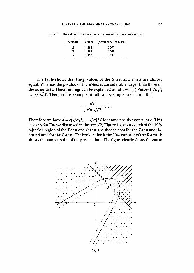
Table 3. The values and approximate p-values of the three test statistics.

Statistic Values p-values of the tests

S 1.293 0.097 T 1.301 0.098 R 1.325 0.235

The table shows that the p-values of the S-test and T-test are almost equal. Whereas thep-value of the R-test is considerably larger than those of the other tests• These findings can be explained as follows: (1) Put n = ( ~ , ..., X/~,66) '. Then, in this example, it follows by simple calculation that

n'! --1.

Therefore we have d - c ( ~ , . . . , x/-~,66) ' for some positive constant c. This leads to S= Tas we discussed in the text; (2) Figure I gives a sketch of the 10% rejection region of the T-test and R-test: the shaded area for the T-test and the dotted area for the R-test. The broken line is the 20% contour of the R-test. P shows the sample point of the present data. The figure clearly shows the cause

T~

- . . • . - - ° • J

I ° ° ° j

s . . . . . . .

I t . . . . . . . .

t j . . . . . . . .

i i . . . . . . , • • , °

/

Fig. 1.

158 K A Z U O A N R A K U ET AL.

of the considerable difference of the p-values between the tests, namely P is almost in the (1, 1) direction which makes the R-test most conservative compared to the T-test. If the sample point were, for example, at Q in the figure, the results would be reversed. In general, the T-test provides smaller p-value than the R-test in the region around the straight line of the (1, 1) direction.

4. Asymptotic comparison of the tests

We first compare the S-test and T-test in Subsection 4.1 by using the Pitman efficiency, then compare the asymptotic powers of the T-test and R-test in Subsection 4.2.

4.1 Comparison o f the S-test and T-test For arbitrary fixed {pg} such that

pL = pO. , p:b = p°.b, a = 1,..., r + 1; b = 1,..., c + 1 ,

we consider the following sequence of alternatives:

Hl,: p~)b = P'b + n-I/26ab , a = 1,..., r + 1; b = 1,..., c + 1 ,

where {3,,b} is a set of real numbers such that

r+l c+l

Z Z &b = 0, a=l b=l

l

N &.<_O, Y. &b_< O, a : l b=l

l = l , . . . , r ; m = l , . . . , c ,

with at least one inequality strict. We shall obtain the Pitman efficiency of the S-test with respect to the

T-test under HI,. It is easy to see that a*m--'a~m in probability as n--.oo, under Hi,, where a~,,

is the (1, m)-element of the covariance matrix Z" generated by the {p'b}. We denote by go tm the (/, m)-element ofL "-1. Also it may be easy to show that, under HI,, S and Tare asymptotically distributed as normal distributions with unit variances and means A~ and A2 respectively as n--.oo, where

A I ~ m

k - = = S l

TESTS FOR THE MARGINAL PROBABILITIES 159

12=- s--I i=I t=l =I

dx/TZ-d

((Wllll[2 [Wlr] 1/2 (W2111/2 [W2clI/21t d = ~ Q 1 ] " ' "~Q,} '~-~2] " '"~Q2] ] "

Then the P i tman efficiency of the S-test relative to the T-test is given by

/ e?(S, T) = I

/12 / '

(see Mitra (1958)). We evaluate ee(S, T) in detail when r = c= 2 andp~. =p.b = 1 / 3, a, b = 1, 2, 3.

Since 8 parameters are involved in/1~ and/12, the numerical comparison would be voluminous unless the parameters are restricted in some way. We shall consider a class of {p~b; a, b= 1, 2, 3} generated by the bivariate normal dis tr ibut ions N(0, 1, I, p), - l < p < l , as follows: Let(U1, U2) be a r andom vector f rom this distribution. Put q~(p)=P( U~>ut/3, U2>ul/3), q2(p) = P(I UII< u~/3, U2>u~/3), q3(p)= P( U~<-u~/3, U2>u~/3) and q4(p)= P(I U~l <ul/3, I U21 <u~/3) where u~/3 is the upper 1 / 3-quantile of the s tandard normal distribution. Then one of {pdb; a, b= 1, 2, 3} satisfying pL=p'.b= 1/3 is given by

[qffp) q2(p) q3(p)) Q= [q2(p) q4(p) q2(p) .

~q3(p) q2(p) qffp)

We consider matrices {fib; a, b= 1, 2, 3} generated f rom Q by repeating the following operation;

(01) interchanging two rows, (02) interchanging two c o l u m n s , (03) interchanging two rows and then two c o l u m n s .

All of the matrices {p~b} generated satisfy the constraint pL =fib--- l / 3. Since qffp)=q3(-p), q2(p)=q2(-p) and q4(p)=q4(-p), such matrices for all - l < p < 1 may be classified into the following 9 types: Put t ing q~=q,(p),

Type 1. ( q l , q2, q3; q2, q4, q2; q3, q2, ql), - l < p < 1 , Type 2. (qt, q2, q3, q3, q2, ql, q2, q4, q 2 ) , - - l < p < 1 , Type 3. (q2, q4, q2; ql, q2, q3; q3, q2, ql), - l < p < l , Type 4. (ql, q3, q2; q2, q2, q4, q3, ql, q 2 ) , - - 1 < p < 1 , Type 5. (q2, ql, q3; q4, q2, q2; q2, q3, q l ) , - - l < p < l ,

160 KAZUO ANRAKU ET AL.

Type 6. (ql, q3, q2; q3, ql, q2, q2, q2, q4) , -- 1 < p < 1 , Type 7. (q4 , q2, q2; q2, ql, q3; q2, q3, ql), -- 1 < p < 1 , Type 8. (q2, ql, q3; q2, q3, qi; q4, q2, q2), - 1 < p < 1 , Type 9. (q2 , q2, q4; q~, q3, q2; q3, ql, q2) , -- 1 < p < 1 .

Here the entries in the parentheses correspond top~l, p12,p13;p21,p2%p23;p3~, p32, p33.

Note that the 9 types of {p~b} with p=-0.9(0.1)0.9 generate altogether 9× 19 sets of {p~b}. Next we select {6ab}. The ee(S, T) depends only on the marginals, i.e., (61., 62, 63.; 3.1, 6.2, 6.3). We specified the following 20 types of (61., 62., 63.; 6.1, 6.2, 6.3) in the calculation.

(1) ( 0 , - 1, 1; 0, 0 , 0 ) , (11) ( - 1 , - 1, 2; 0 , - 1, 1), (2) ( 0 , - 1 , 1; 0 , - 1 , 1), (12) ( - 1 , - 1 , 2 ; - 1 , 0 , 1 ) , (3) ( - 1 , 0, 1; 0, 0 , 0 ) , (13) ( - l , - 1, 2 ; - 1, 1 ,0 ) , (4) ( - l, 0, 1; 0 , - l, l ) , (14) ( - l , - l, 2 ; - 1 , - 1 ,2 ) , (5) ( - 1, 0, 1 ; - 1, 0, 1), (15) ( - 2 , 1, 1; 0, 0 , 0 ) , (6) ( - 1, 1, 0; 0, 0, 0), (16) ( - 2 , 1, 1; 0 , - 1, 1), (7) ( - 1, 1, 0; 0 , - 1, 1), (17) ( - 2 , 1, 1 ; - 1, 0, 1), (8) ( - l, 1, 0 ; - 1, O, 1), (18) ( - 2 , 1, 1 ; - 1, 1, O), (9) ( - 1, 1, 0 ; - 1, 1 ,0) , (19) ( - 2 , 1, 1 ; - l , - 1 ,2 ) ,

(10) ( - 1 , - 1, 2; 0, 0 , 0 ) , (20) ( - 2 , 1, 1 ; - 2 , 1, 1).

Thus, altogether 9× 19×20=3420 sets of {p~b); a, b= 1, 2, 3} are generated. It was found that among these 3420 sets, 540 sets led to ee(S, T)= 1 and 1432 sets led to ee(S, T)> 1. Table 4 summarizes the values ofee(S, T). The table shows that the T-test competes well with the S-test. We found by calculation that when the sample size is large enough, the S-test satisfies the condition (2.3) for all set of {fib} generated.

Table 4. The distribution of ee(S, T).

ee(S, T) 0.75 0.85 0.85 0.95 0.95-1.05 1.05-1.15 1.15-1.25 Total

Frequency 6 142 3131 134 7 3420

4.2 Comparison of the T-test and R-test We next compare the T-test and R-test. Under the sequence of the

alternative hypothesis Hln described in the last section it follows that the random vector (TI, T2) converges in law to ( U~, U2) which is distributed as a bivariate normal distribution N2(z~, zz, 1, 1, p) where

TESTS F O R T H E M A R G I N A L P R O B A B I L I T I E S 161

T2 ~ ~ ~ tW2rnl 1/2 m=,~=, I--~--~ J & '

and p is given in (2.4). F r o m this the asymptot ic power of the T-test, asymp- totically with level a, is given by

1 - ¢ > ( u ~ - r~ + r2 ]

On the other hand, following Bar tholomew (1961) and Chatterjee and De (1972), the corresponding asymptotic power of the R-test is given by

[1 - ¢'(ca - 2 cos ~)],/'( - 2 sin ()

+ [1 - ~(ca - 2 cos (~' - ~))]~( - 2 sin (~u - ~))

1 ~ { 1 Z2 + f,,o e x p - + - cos 0)} drdO ,

where

k = (1 - p2)-l/2(r2 + r 2 - 2pT12"2) 1/2 ,

~, = cos-~( _ p ) , "[" 2 = cos-~[(r~ - p 2)/(r, + r~ - 2p~1r2) '/2]

Fixing a, p and 2, and denot ing the asymptot ic powers of the T-test and R-test by f i r ( l ) and fiR(i), we consider the powers as functions of (. It is s t raightforward to see that both f i r ( l ) and fiR(l) attain their m a x i m u m values at ~=~u/2, symmetrically decrease as 1¢-~'/21 increases and attain their min imum values at ~=0 or ~,. Note that ( = 0 , ~u/2, ~u correspond to r2=0, r~ =r2 and r l = 0 respectively, and that the vector O~=cZd(c>O), to which the T-test is a uniformly most powerful in an asymptotic sense, implies r~ =r2. We studied the behavior of f ir(() and fiR(l) for selected values of a, 2 and p. Figure 2 illustrates the case when a=0.05; 2=2; p-- -0 .5 , 0.0, 0.5. The figure shows that the T-test is superior to R-test a round rl =r2, but inferior a round ~ =0 or ~2=0. Incidentally, this reinforces the finding in the example in the previous section. The figure also shows that the superiority of the T-test a round rl =r2 increases as the value o fp decreases; that the power of the R-test is fairly stable for various directions of the alternatives. These findings are unalterd for different values of 2 and a.

5. Concluding r e m a r k s

In this paper we have discussed the problem of testing pa. =p:. , p.b=p.%

162 KAZUO A N R A K U ET AL.

0.6

0.4

0.2

0

fl~(~)

~R(()

6 (i) p=-0.5

0.6

0.4

0.2

7~ - - (¢) 3

0.6

0.4

0.2

#r(~) 0.6

0.4

0.2

(ii) 4 p=O.O

/t - - ( ¢ 3 2

Fig. 2.

0.6

0.4

0.2

0

3 (iii) p=0.5

0.6

0.4

0.2

2__._~_~ (~ 3

Asymptotic powers fir(O and fla(~) for a=0.05; 2=2; p = - 0 . 5 , 0.0, 0.5.

1 1 m m for a= l , . . . , r, b= l , . . . , c against alternatives ~Epa. <_~_ pa., ° b~= P'b<-- b~= p.b,° for

l= 1,..., r, m = 1,.. . ,c, with at least one inequality strict. The problem is not only interesting by itself as a testing hypothesis in a contingency table, but also it has been shown in this paper that the alternative hypothesis is related to the one-sided alternative in a comparative study under a bivariate nonparametric formulation.

We have considered the three tests, S-test, T-test and R-test. The S-test is an approximately most stringent somewhere most powerful test. The T-test

TESTS FOR THE MARGINAL PROBABILITIES 163

and R-test combine approximately most stringent somewhere most powerful tests obtained from each marginal of the contingency table. Whereas the T-test simply adds, R-test employs the likelihood ratio criterion for the combination.

The alternative hypothesis is composite with restriction and it is difficult to compare the three tests in general. We have considered the restricted family of alternative hypothesis which is generated by a bivariate normal distribution for the comparison of the S-test and T-test. Also we have directly compared the asymptotic powers of the T-test and R-test. Under these setups it has been shown that the three tests are competitive regarding their asymptotic powers, in particular

i) T-test is highly competitive with the S-test. ii) T-test is superior to the R-test around E(T1) = E(T2), but inferior to the

R-test around E(T0=0 or E(T2)=0. iii) The superiority of the T-test around E(TO=E(T2) increases as the

correlation of T~ and T2 decreases. iv) The power of the R-test is fairly stable for various directions of the

alternatives. We could not compare the powers of the S-test and T-test directly

because of the involvement of too many parameters. The usefulness of the tests has been shown by the practical data from a

case-control study. It has been shown that the T-test has smallerp-values than the R-test in the region around the straight line, TI-- T2.

Acknowledgement

The authors are grateful to the referee for valuable comments which improved the representation of this paper.

REFERENCES

Bartholomew, D. J. (1961). A test of homogeneity of means under restricted alternatives (with discussion), J. Roy. Statist. Soc. Ser. B, 23, 239-281.

Chatterjee, S. K. and De, N. K. (1972). Bivariate nonparametric location tests against restricted alternatives, Calcutta Statist. Assoc. Bull., 21, 1-20.

Kud6, A. (1963). A multivariate analogue of the one-sided test, Biometrika, 50, 403-418. Mitra, S. K. (1958). On the limiting power function of the frequency chi-square test, Ann.

Math. Statist., 29, 1221-1233. Rao, C. R. (1973). Linear Statistical Inference and Its Applications, 2nd ed., Wiley, New York. Schaafsma, W. (1966). Hypothesis Testing Problems with the Alternative Restricted by a

Number of Inequalities, Noordhoff, Groningen. Schaafsma, W. and Smid, L. J. (1966). Most stringent somewhere most powerful tests against

alternatives restricted by a number of linear inequalities, Ann. Math. Statist., 37, 1161- 1172.