Embed Size (px)
Citation preview

Analysis of Nutrient Dynamics in Roxo Catchment Using Remote Sensing Data and
Numerical Modeling
Imesh Chanaka Bihawala Vithanage March, 2009

Analysis of Nutrient Dynamics in Roxo Catchment Using Remote Sensing Data and Numerical Modeling
by
Imesh Chanaka Bihawala Vithanage
Thesis submitted to the International Institute for Geo-information Science and Earth Observation in partial fulfilment of the requirements for the degree of Master of Science in Geo-information Science and Earth Observation. Specialisation: Integrated Watershed Modeling and Management. Thesis Assessment Board Professor Dr. Z. Bob Su, Chairman, WREM Department, ITC Dr. Ir. D.C.M. Augustijn, External Examiner, WEM Department, UT Dr. Ir C.M.M. Chris Mannaerts, First Supervisor, WREM Department, ITC Dr. B.H.P. Maathuis, Second Supervisor, WREM Department, ITC M. Yevenes, Advisor, WREM Department, ITC
INTERNATIONAL INSTITUTE FOR GEO-INFORMATION SCIENCE AND EARTH OBSERVATION
ENSCHEDE, THE NETHERLANDS

Analysis of Nutrient Dynamics in Roxo Catchment Using Remote Sensing data and Numerical Modeling
Disclaimer This document describes work undertaken as part of a programme of study at the International Institute for Geo-information Science and Earth Observation. All views and opinions expressed therein remain the sole responsibility of the author, and do not necessarily represent those of the institute.

Analysis of Nutrient Dynamics in Roxo Catchment Using Remote Sensing data and Numerical Modeling
i
Abstract
The water quality in catchments is influenced by the complex combinations of land use, point sources combined with weather and other natural and human influences. Agricultural non point source pollution is usually considered a major cause of water quality deterioration in larger agricultural catchments. Farmers usually tend to use more fertiliser with the intention of making more harvest without considering the optimum doses, and their effects on the environment. Excess nutrients leached through the watershed and are collected on the downstream water bodies, making them eutrophic, being excessive algae and/or plant growth due to an abundance of nutrients. The excess growth of algae and phytoplankton has various deleterious effects of the water storage and distribution systems like clogging of filters, reduction of dissolved oxygen (DO), unpleasant taste and odour. Some algae species (e.g., blue green algae) may be toxic to fish, animals (like birds) and even humans (Chapra, 1997). In addition ammonia (NH3), nitrates (NO3) and nitrites (NO2) can be harmful when present in excessive amounts in water. In this study, our aim was to research the hydrological and environmental processes associated with Nitrogen (N) and Phosphorous (P) compounds and their dynamics in the hydrological system of the Roxo catchment. A model is developed that simulates the catchment flow hydraulics and the water quality in the catchment and Roxo reservoir. A special effort was put in place to model the effects of the Beja city waste water treatment plant (WWTP) as a test case for the model. This WWTP is an identified nutrient point source in the upper catchment. The hydrological, physical and biochemical water quality processes have been developed using Duflow Modeling Studio (DMS) including its Rainfall Runoff component model (RAM), based on linear reservoir theory. RAM elements (runoff areas) permit simulation of runoff hydrograph at the detailed sub-catchment level and permit to simulate distributed nutrient source (N, P) apportionment of agricultural areas to streams. Because no direct stream flow gauging station was present existing in the upper Roxo, a reservoir water balance technique was used to estimate daily catchment stream flow to the reservoir. An extensive data set was available for this purpose. The hydrological model calibration and validation was based on this, was judged satisfactory. During summer periods, some small negative inflows were computed. These small estimation errors were considered due the precision in the level measurements, as well as uncertainties in some water abstraction values (extra unregistered withdrawals) or losses (evaporation, groundwater) from the reservoir especially during summer periods. The flow calibration of DMS was finally performed using cumulative decadal inflow values. Besides running of the DMS model using interpolations from daily rain gauge data, we have run the model with remote sensing derived rainfall data (i.e. the Meteosat Multi-sensor Precipitation Estimate or MSG-MPE). We used a density of 18 data extraction points to represent catchment rainfall inputs. A simulation period starting from Jan 2007 to May 2008 with daily time steps was used for the purpose, and was a function of the availability of the MSG satellite rainfall data products. The study showed that the MSG daily rainfall data is not properly correlated with the daily gauge precipitation records. However when compared with the entire period, the cumulative result showed good agreement with the

ii
aggregated gauge station total rainfalls. The hydrologic responses produced using MPE showed that there are discrepancies with runoff hydrographs and this can be explained by the occasional high magnitude rainfalls recorded in the MPE that are significantly different from the gauge records. After calibration and validation of the flow model, and comparison of the rainfall runoff response using ground gauged rainfall and satellite precipitation inputs, nutrient export from the agriculture areas, and the impact of a point source (i.e., the WWTP) was simulated. These first results were interpreted and compared to observed stream and reservoir water quality data. Although, initial water quality modeling results are encouraging, and confirmed we were able to simulate the magnitudes and local spatial and temporal variations of the nutrient processes, much more model and parameter uncertainties need to be eliminated before the water quality model can be judge as appropriate for the upper Roxo catchment and the reservoir system. This can be obtained through further study and research.

Analysis of Nutrient Dynamics in Roxo Catchment Using Remote Sensing data and Numerical Modeling
iii
Acknowledgements
First and the foremost I am grateful to my employer National Water Supply and Drainage Board, Sri Lanka for allowing me to take this valued long-term fellowship to pursue with Master of Science Degree. At the same time I am thankful to ITC for offering me this esteemed MSc degree programme and also providing me with a scholarship for financing all expenses during 18 months period. I express my heartiest appreciation to my 1st supervisor Dr Ir. C.M.M Mannaerts for the support and guidance extended to me during this whole research period. The encouragement and the critical reviews had immensely helped in shaping up the thesis to the due expectations. Further, during the field campaign at Portugal, Chris’s assistance was enormous as he had not limit himself just a supervisor’s task but guided us at all possible occasions to get the maximum out of field visit. I would also acknowledge the Dr B.H.P Maathuis, my 2nd supervisor. He often supported me at critical junctures when struggling with technical issues. At the same time I am grateful to Drs J.B de Smeth for providing space at the laboratory and supplying ancillary logistics for performing water sample analysis and the supervision over performing water quality testing in due manner. I would also like to remember the Technical Director I. Oliveira and his staff of COTR, Engineer Alexandre Leal of EMAS, The Director ABROXO and Engineer R. Nobre from IPB (Beja) for the corporation extended to us in providing essential information for the success of this research study. I am also thankful to Mariella, Murat and colleagues Fransiska, Prescilla and Daphne, who were with me during the field campaign and for working as a team in attending the objectives. Moreover they made the field campaign more enjoyable. I would also like to acknowledge the lecturers of the WREM programme, whom made me equipped with proper tools and techniques to proceed with the research work. It is also essential to thank ITC library in providing essential information and resources, when I made a simple request to them. I also wish to thank all my friends in the WREM 2008 for giving suggestions, thoughtful reviews during this research phase. Last but not least, I would like to express my sincere gratitude to my family, Niroshini, Iresh and Harshi for the moral support and love they have showed me during this long duration I was away from them. Especially the tolerance they have showed during this tough time made this task possible for me and to concentrate more on my studies. Finally I wish thank my parents for supporting me in all possible ways and looking after my family with utmost care during this 18 months period.

iv
Table of contents
1. Introduction.................................................................................................................................1 1.1. Background......................................................................................................................1 1.2. Research problem.............................................................................................................2 1.3. Objectives ........................................................................................................................3 1.4. Research questions ...........................................................................................................3 1.5. Research hypothesis .........................................................................................................3 1.6. Description of the study area ............................................................................................4 1.7. Climate ............................................................................................................................5
1.7.1. Temperature.......................................................................................................5 1.7.2. Precipitation and Evapotranspiration ..................................................................6 1.7.3. Topography........................................................................................................6 1.7.4. Hydrology..........................................................................................................6 1.7.5. Land use ............................................................................................................7
2. Materials and Methods ................................................................................................................9 2.1. Work plan ........................................................................................................................9
2.1.1. Pre-field work ....................................................................................................9 2.1.2. Field work..........................................................................................................9 2.1.3. Post-field work...................................................................................................9
2.2. Remote sensing data .......................................................................................................10 2.2.1. ASTER pre-processed digital elevation model (DEM).......................................10 2.2.2. Multi-sensor Precipitation Estimates (MPE ) ....................................................10
2.3. Data collection from Beja water authorities .....................................................................11 2.4. Field data collection........................................................................................................11
2.4.1. Geo-referencing data ........................................................................................ 12 2.4.2. Data collection for CORINE land cover accuracy assessment............................ 12 2.4.3. Stream section details ....................................................................................... 12 2.4.4. Water sample collection....................................................................................12
3. Data Analysis and Integration....................................................................................................15 3.1. ASTER DEM ................................................................................................................15 3.2. Meteorological information............................................................................................. 18
3.2.1. Rainfall estimation ........................................................................................... 18 3.2.2. Evapotranspiration estimation...........................................................................20
3.3. Data preparation for reservoir water balance...................................................................22 3.3.1. Inflow ..............................................................................................................23 3.3.2. Outflow............................................................................................................23 3.3.3. Estimation of rainfall & evaporation volumes....................................................23
3.3.3.1. Stage volume, Stage surface area relationships ................................ 24 3.3.3.2. Water surface evaporation............................................................... 25 3.3.3.3. Direct rainfall (input) ......................................................................26
3.3.4. Spill occurrences .............................................................................................. 27 3.3.5. Change in storage-Roxo reservoir .....................................................................28
Analysis of Nutrient Dynamics in Roxo Catchment Using Remote Sensing data and Numerical Modeling
v
3.3.6. Water abstractions............................................................................................28 3.4. Water balance and Estimation of inflows........................................................................28 3.5. Water quality data ..........................................................................................................30
3.5.1. In-situ water tests .............................................................................................30 3.5.2. Laboratory analysis ..........................................................................................31 3.5.3. Analysis of results ............................................................................................32
3.6. Flow measurements ........................................................................................................33 3.7. Soil data .........................................................................................................................33 3.8. Land cover data ..............................................................................................................34 3.9. Historical water qauality data .........................................................................................35
4. Numerical Modeling ..................................................................................................................37 4.1. Duflow Modeling Studio (DMS).....................................................................................37 4.2. Duflow flow model .........................................................................................................37 4.3. Duflow quality model .....................................................................................................38 4.4. Duflow rainfall runoff (RAM) component .......................................................................39
4.4.1. Open water surface...........................................................................................41 4.4.2. Paved surface ...................................................................................................41 4.4.3. Unpaved surfaces .............................................................................................43
4.5. RAM quality model (DUFLOW, 2004b).........................................................................44 4.6. Quality model definition..................................................................................................45 4.7. Previous modeling studies with Duflow...........................................................................46 4.8. Model simplifications and limitations (DUFLOW) ..........................................................47
5. Integration of satellite remote sensing data .................................................................................49 5.1. MSG_Multi-sensor Precipitation Estimate (MPE) ...........................................................49 5.2. MPE precipitation data ...................................................................................................49 5.3. Data formats and pre-processing.....................................................................................50 5.4. Data extraction...............................................................................................................50 5.5. Spatial variability of the rainfall with in the catchment ....................................................53 5.6. Comparison of MPE rainfall with gauge data ..................................................................54 5.7. Conclusion .....................................................................................................................54
6. Model Development and Implementation....................................................................................55 6.1. Modeling objectives and the scope...................................................................................55 6.2. Schematization of the study area .....................................................................................55 6.3. Basic data inputs and data formats..................................................................................56 6.4. Initial and Boundary conditions.......................................................................................57 6.5. Sensitivity analysis .........................................................................................................59 6.6. Model calibration............................................................................................................60 6.7. Model validation.............................................................................................................60 6.8. Results-water quality (nutrient) modeling ........................................................................62 6.9. Scenario analysis ............................................................................................................63
7. Conclusion and recommendation................................................................................................67 7.1. Conclusion .....................................................................................................................67
7.1.1. Estimation of runoff..........................................................................................67 7.1.2. Numerical flow and water quality Modeling ......................................................67

vi
7.1.3. Integration of rainfall remote sensing data in Duflow.........................................68 7.2. Recommendation............................................................................................................69
References ........................................................................................................................................71 Appendixes Appendix 1 Research phases and key activities ....................................................................76 Appendix 2 Maps ...............................................................................................................77 Appendix 3 Potential water surface evaporation calculation (sample calculation sheet).........79 Appendix 4 Data constancy checks using double mass technique..........................................80 Appendix 5 Land cover .......................................................................................................82 Appendix 6 Data for crop evapotranspiration estimates ....................................................... 84 Appendix 7 Roxo Stage Volume curve (Mannaerts , 2006) ..................................................85 Appendix 8 Soil Information ............................................................................................... 86 Appendix 9 MSG MPE data gaps ....................................................................................... 88 Appendix 10 Field data collection for water quality ............................................................... 89 Appendix 11 Salt dilution gauging......................................................................................... 91 Appendix 12 Water consumption/abstraction data (sample) ...................................................92 Appendix 13 Collected ground control points for Geo-referencing..........................................93 Appendix 14 Historical water quality data .............................................................................94 Appendix 15 Water quality description (Nutrients) ................................................................ 96 Appendix 16 Water balance calculation.................................................................................98 Appendix 17 Results of the sensitivity analysis .................................................................... 100 Appendix 18 RAM surface parameters and calibrated parameter settings............................. 102 Appendix 19 Temporal Phosphates concentration and load variation at reservoir section ...... 103
Analysis of Nutrient Dynamics in Roxo Catchment Using Remote Sensing data and Numerical Modeling
vii
List of figures
Figure 1-1 Geographical location of the Roxo catchment ......................................................4 Figure 1-2 Variation of mean daily temperatre over the two weather (Beja , Aljustrel) stations ..........................................................................................................................5 Figure 1-3 Variation of precipitation and reference crop evapotranspiration..........................6 Figure 2-1 Water sampling locations..................................................................................13 Figure 2-2 Different land cover types observed in the Roxo catchment................................14 Figure 3-1 SNIRH station points considered in accuracy assessment ..................................16 Figure 3-2 Accuracy assessment of the ASTER DEM........................................................16 Figure 3-3 DEM hydro processing procedure for hydrologic parameter extraction ..............17 Figure 3-4 Cumulative ETo comparison of the two COTR weather stations.........................20 Figure 3-5 Weighted crop factors (Kc) for catchment #01 ...................................................21 Figure 3-6 Important terms of the water balance of a reservoir ...........................................22 Figure 3-7 Stage area relationship for the Roxo reservoir ...................................................24 Figure 3-8 Albufeira Do Roxo floating station ...................................................................25 Figure 3-9 Double mass graph between Beja and Albufeira stations....................................27 Figure 3-10 Basic configuration of the Ogee type crest spillway extracted from (Khatsuria, 2005) ........................................................................................................................27 Figure 3-11 Monthly runoff estimation and the rainfall graph for the simulation period (2001-2007) ........................................................................................................................29 Figure 3-12 Nitrification process along the river...................................................................32 Figure 4-1 Duflow RAM modeling framework (DUFLOW, 2004b)....................................40 Figure 4-2 Chemical and water quality processes modelled in RAM (DUFLOW, 2004b) ....44 Figure 4-3 Nitrogen cycle ..................................................................................................45 Figure 4-4 Phosphor cycle .................................................................................................45 Figure 4-5 Structure of the water quality model description ................................................46 Figure 5-1 Roxo catchment with 18 pts overlaid on top of MPE image: date 10/02/2007 ....51 Figure 5-2 Comparison of MPE data and ground based data ..............................................51 Figure 5-3 Consistency check for random 5 points..............................................................53 Figure 6-1 Model calibration: simulated discharge vs. observed runoff ...............................61 Figure 6-2 Model validation: simulated discharge vs. observed runoff...............................61 Figure 6-3 Duflow model structure showing all key elements..............................................62 Figure 6-4 Nitrification along the main river (Chamine) section .........................................62 Figure 6-5 Temporal variation of the nitrate, ammonium concentrations .............................64 Figure 6-6 Nutrient concentrations in the Roxo reservoir according to EMAS data .............65 Figure 6-7 Runoff simulation based on the two rainfall inputs ............................................66
viii
List of tables
Table 1-1 COTR automatic weather stations in the vicinity of Roxo catchment ...................5 Table 1-2 Monthly average temperature over last seven years .............................................5 Table 1-3 Monthly average reference crop evapotranspiration and precipitation ..................6 Table 1-4 Land cover based on the European CORINE 2000 classification .........................7 Table 2-1 Water authorities visited during the field visit....................................................11 Table 3-1 List of weather stations in the vicinity of the catchment .....................................19 Table 3-2 Interpolation weights for Thiessen polygon method ...........................................19 Table 3-3 Interpolation weights for Inverse distance method..............................................19 Table 3-4 Crop factors for different crop types .................................................................21 Table 3-5 Growing stages (days) ......................................................................................21 Table 3-6 Landsat ETM + images used in extending the stage area relationship Roxo .......24 Table 3-7 Details of the weather stations located close to Roxo reservoir........................... 25 Table 3-8 Field test results ............................................................................................... 31 Table 3-9 Results of the laboratory analysis .....................................................................32 Table 3-10 Major soil types in the Roxo catchment............................................................. 34 Table 3-11 Reclassification of CORINE land cover classes to DUFLOW RAM..................35 Table 5-1 Cumulative rainfall figures ...............................................................................52 Table 6-1 Shows the data required for the model............................................................... 57 Table 6-2 Typical values of concentrations of nutrients.....................................................58 Table 6-3 RAM sensitivity analysis results .......................................................................59

Analysis of Nutrient Dynamics in Roxo Catchment Using Remote Sensing data and Numerical Modeling
1
1. Introduction
1.1. Background
The water quality is a complex combination of land use, point sources, natural processes in each catchment (Chen et al., 2005). The sewage treatment effluents and agricultural sources are respectively the main contributors to phosphorus and nitrates in water bodies (Neal et al., 2008). The nitrogen (N) and phosphorus (P) are the two essential nutrients required for the growth of plant life. Nitrogen exists in different oxidation forms Nitrate (NO3
-), Nitrite (NO2-), Ammonium (NH4
+), Organic Nitrogen, Molecular Nitrogen (N2), Nitrous Oxides (N2O) in the environment (Chapman, 1996). There are different sources contributing nutrients to the lake/reservoir water systems and it could be originating from the use of fertilizer, the mineralization of dead plant and animals, effluent from the urban and waste water treatment systems and water flows through igneous rock sources (Chapman, 1996). In the last few decades, human activities have enhanced the enrichment of water bodies with nutrients, (Leston et al., 2008) particularly nitrogen and phosphorus. Phytoplankton and macro algae are capable of taking the advantage of the available resources in transient environments. Their high surface area to volume ratio and high affinity for nutrients, especially N and P, favour a rapid nutrient uptake and high growth and production rates leading to very large biomass values (Leston et al., 2008). The biological response to excess nutrient input to the water system is referred to as the Eutrophication (Chapman, 1996). Nutrient inputs generally are increased by human-induced land use changes specially the intense farming practices can lead to eutrophication and impairment of surface water quality (Dodds and Oakes, 2006) The factors affecting the growth of phytoplankton are temperature, light and the nutrients, when each of these contributing factors comes to its optimum level there could be out break of heavy algal blooms (Alam et al., 2001). There are numerous adverse effects with the phytoplankton, water becomes turbid making the water more turbid, this can reduce the photosynthetic activities of the aquatic plant and ultimately causing the extinction of aquatic life forms. The effects of land use and land use changes in a catchment are key aspects to understand the stream/catchment nutrient dynamics. Further the effect of rain events and the seasonality of nutrient dynamics are of interest to assess the maximum nutrient inflows in to an important water body and the associated delay after particular event are factors that affect the temporal water quality. The Nutrient dynamics is also dependent heavily on the application pattern of fertilizer in agricultural catchments (Poor and McDonnell, 2007).
2
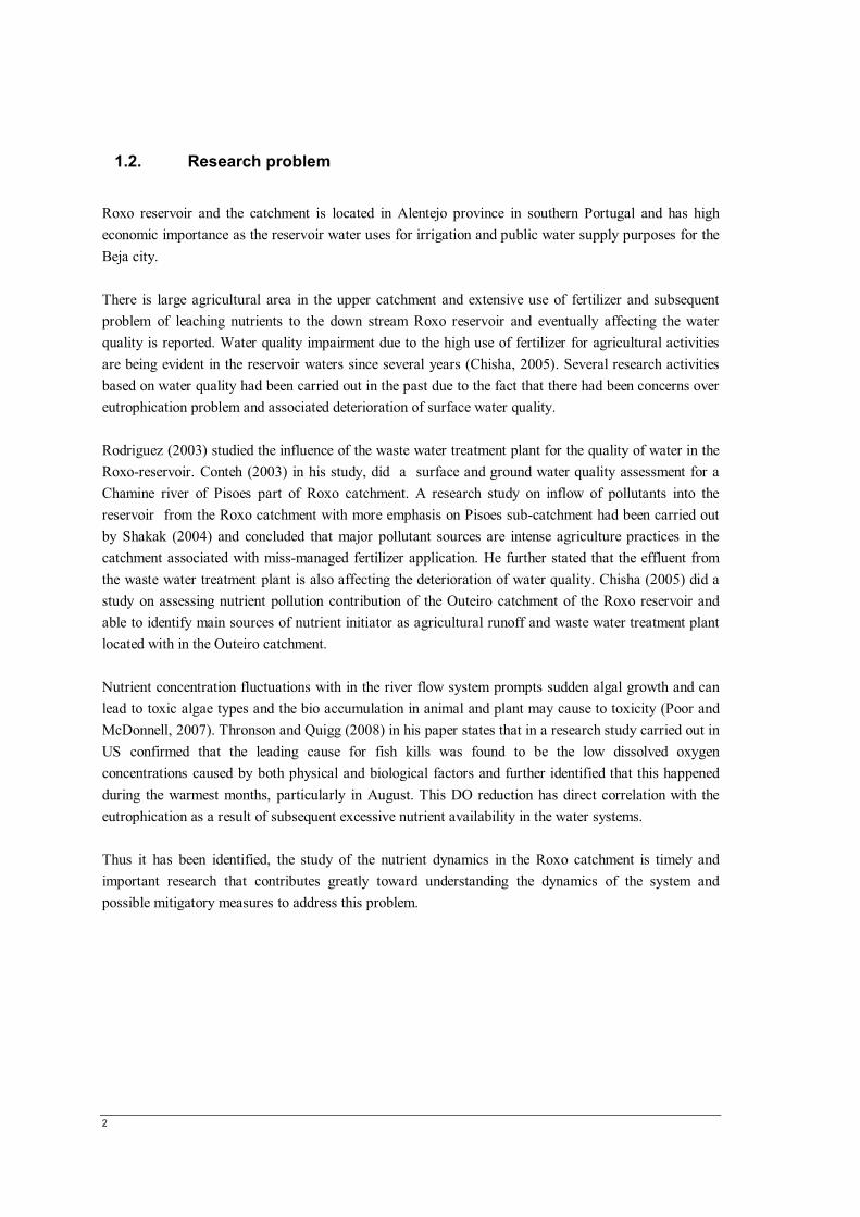
1.2. Research problem
Roxo reservoir and the catchment is located in Alentejo province in southern Portugal and has high economic importance as the reservoir water uses for irrigation and public water supply purposes for the Beja city. There is large agricultural area in the upper catchment and extensive use of fertilizer and subsequent problem of leaching nutrients to the down stream Roxo reservoir and eventually affecting the water quality is reported. Water quality impairment due to the high use of fertilizer for agricultural activities are being evident in the reservoir waters since several years (Chisha, 2005). Several research activities based on water quality had been carried out in the past due to the fact that there had been concerns over eutrophication problem and associated deterioration of surface water quality. Rodriguez (2003) studied the influence of the waste water treatment plant for the quality of water in the Roxo-reservoir. Conteh (2003) in his study, did a surface and ground water quality assessment for a Chamine river of Pisoes part of Roxo catchment. A research study on inflow of pollutants into the reservoir from the Roxo catchment with more emphasis on Pisoes sub-catchment had been carried out by Shakak (2004) and concluded that major pollutant sources are intense agriculture practices in the catchment associated with miss-managed fertilizer application. He further stated that the effluent from the waste water treatment plant is also affecting the deterioration of water quality. Chisha (2005) did a study on assessing nutrient pollution contribution of the Outeiro catchment of the Roxo reservoir and able to identify main sources of nutrient initiator as agricultural runoff and waste water treatment plant located with in the Outeiro catchment. Nutrient concentration fluctuations with in the river flow system prompts sudden algal growth and can lead to toxic algae types and the bio accumulation in animal and plant may cause to toxicity (Poor and McDonnell, 2007). Thronson and Quigg (2008) in his paper states that in a research study carried out in US confirmed that the leading cause for fish kills was found to be the low dissolved oxygen concentrations caused by both physical and biological factors and further identified that this happened during the warmest months, particularly in August. This DO reduction has direct correlation with the eutrophication as a result of subsequent excessive nutrient availability in the water systems. Thus it has been identified, the study of the nutrient dynamics in the Roxo catchment is timely and important research that contributes greatly toward understanding the dynamics of the system and possible mitigatory measures to address this problem.

Analysis of Nutrient Dynamics in Roxo Catchment Using Remote Sensing data and Numerical Modeling
3
1.3. Objectives
In order to address the research problem of studying the dynamics of the nutrients in the Roxo catchment, it was decided to build a numerical model using the Duflow Modeling Studio (DMS) with rainfall runoff components (RAM). The main objectives of the research study can be listed as follows;
• Build an operational numerical water quality model for the Roxo catchment using Duflow Modeling Studio (DMS) and rainfall runoff (RAM) components
• Perform model Calibration and Validation through reservoir water balancing technique as no in-
stream discharge measurements available
• Utilization of satellite remote sensing precipitation data as model input and compare the performance with the gauge station precipitation records
1.4. Research questions
In addressing the above objectives, following research questions had been identified and efforts were made to answer the subsequent research questions during the research phase.
• Can the watershed water quality model be build using DMS with RAM component and can it efficiently represents the water quality and nutrient dynamics of the Roxo catchment?
• What kind of temporal and special variation of nutrient concentrations could be observed with
in the catchment?
• Whether the reservoir water balance technique provides stream inflows that can be used for hydrologic model calibration and validation
• What type of satellite sensors data can effectively be used for watershed water quality model? • Whether the use of two precipitation input methods will provide significant differences in
results?
1.5. Research hypothesis
The following are hypothesized in order to proceed with the research work
• The hydrological model developed using DMS for the Roxo catchment can be calibrated and validated effectively by the inflows calculated using the reservoir water balance technique.
• The land use conditions in riparian zones are highly correlated with in-stream and reservoir
nutrient concentrations.
4
1.6. Description of the study area
The Beja district is having approximately population of 165,000 with in an area of 10,224 km2. Beja municipality is the capital of Beja district and there is about 35,000 population lives in 18 communes of an area of 1140 km2 in the municipality with low population density of 31 per km2 (FOTW, 2009).
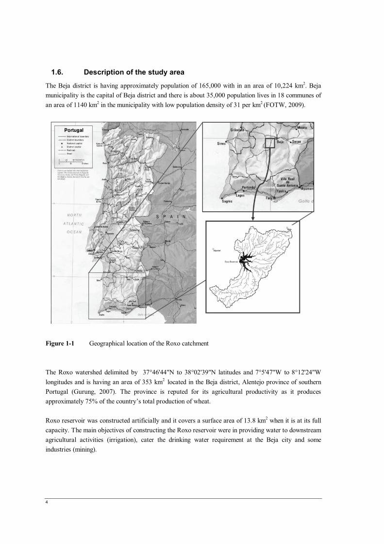
Figure 1-1 Geographical location of the Roxo catchment The Roxo watershed delimited by 37°46'44"N to 38°02'39"N latitudes and 7°5'47"W to 8°12'24"W longitudes and is having an area of 353 km2 located in the Beja district, Alentejo province of southern Portugal (Gurung, 2007). The province is reputed for its agricultural productivity as it produces approximately 75% of the country’s total production of wheat. Roxo reservoir was constructed artificially and it covers a surface area of 13.8 km2 when it is at its full capacity. The main objectives of constructing the Roxo reservoir were in providing water to downstream agricultural activities (irrigation), cater the drinking water requirement at the Beja city and some industries (mining).
Analysis of Nutrient Dynamics in Roxo Catchment Using Remote Sensing data and Numerical Modeling
5
1.7. Climate
1.7.1. Temperature
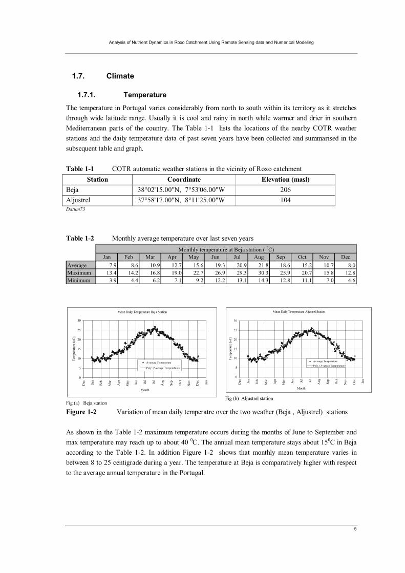
The temperature in Portugal varies considerably from north to south within its territory as it stretches through wide latitude range. Usually it is cool and rainy in north while warmer and drier in southern Mediterranean parts of the country. The Table 1-1 lists the locations of the nearby COTR weather stations and the daily temperature data of past seven years have been collected and summarised in the subsequent table and graph. Table 1-1 COTR automatic weather stations in the vicinity of Roxo catchment
Station Coordinate Elevation (masl) Beja 38°02'15.00"N, 7°53'06.00"W 206 Aljustrel 37°58'17.00"N, 8°11'25.00"W 104 Datum73
Table 1-2 Monthly average temperature over last seven years
Jan Feb Mar Apr May Jun Jul Aug Sep Oct Nov DecAverage 7.9 8.6 10.9 12.7 15.6 19.3 20.9 21.8 18.6 15.2 10.7 8.0Maximum 13.4 14.2 16.8 19.0 22.7 26.9 29.3 30.3 25.9 20.7 15.8 12.8Minimum 3.9 4.4 6.2 7.1 9.2 12.2 13.1 14.3 12.8 11.1 7.0 4.6
Monthly temperature at Beja station ( oC)
Mean Daily Temperature Beja Station
0
5
10
15
20
25
30
Dec Jan
Feb
Mar
Apr
May Ju
n Jul
Jul
Aug
Sep
Oct
Nov Dec Jan
Month
Tem
pera
ture
(oC
)
Average Temperature
Poly. (Average Temperature)
Fig (a) Beja station
Mean Daily Temperature Aljustrel Station
0
5
10
15
20
25
30
Dec Jan
Feb
Mar
Apr
May Jun Jul
Jul
Aug Sep
Oct
Nov Dec Jan
Month
Tem
pera
ture
(oC
)
Average Temperature
Poly. (Average Temperature)
Fig (b) Aljustrel station
Figure 1-2 Variation of mean daily temperatre over the two weather (Beja , Aljustrel) stations As shown in the Table 1-2 maximum temperature occurs during the months of June to September and max temperature may reach up to about 40 0C. The annual mean temperature stays about 150C in Beja according to the Table 1-2. In addition Figure 1-2 shows that monthly mean temperature varies in between 8 to 25 centigrade during a year. The temperature at Beja is comparatively higher with respect to the average annual temperature in the Portugal.
6
1.7.2. Precipitation and Evapotranspiration
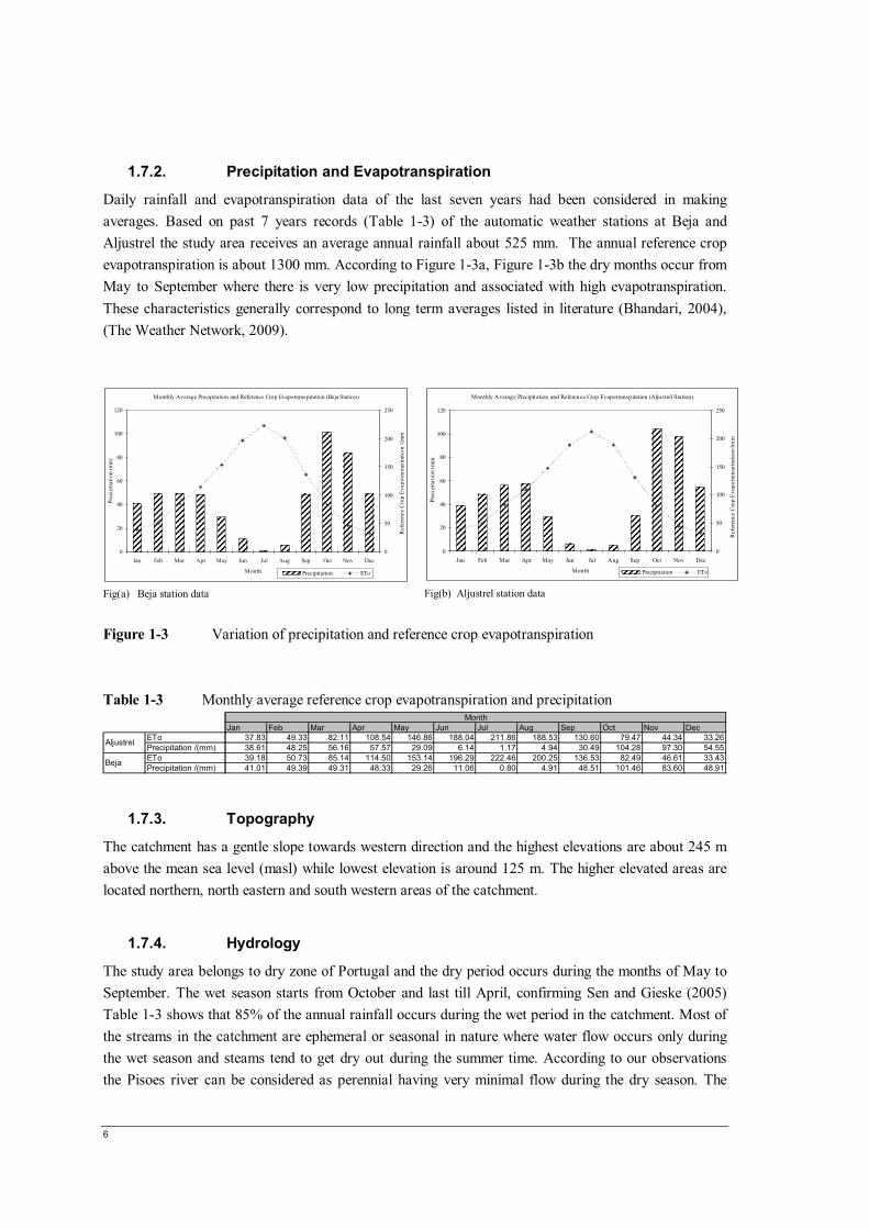
Daily rainfall and evapotranspiration data of the last seven years had been considered in making averages. Based on past 7 years records (Table 1-3) of the automatic weather stations at Beja and Aljustrel the study area receives an average annual rainfall about 525 mm. The annual reference crop evapotranspiration is about 1300 mm. According to Figure 1-3a, Figure 1-3b the dry months occur from May to September where there is very low precipitation and associated with high evapotranspiration. These characteristics generally correspond to long term averages listed in literature (Bhandari, 2004), (The Weather Network, 2009).
Monthly Average Precipitation and Reference Crop Evapotranspiration (Beja Station)
0
20
40
60
80
100
120
Jan Feb Mar Apr May Jun Jul Aug Sep Oct Nov Dec
Month
Prec
ipita
tion
(mm
)
0
50
100
150
200
250R
efer
ence
Cro
p Ev
apot
rans
pira
tion
/(mm
Precipitation ETo Fig(a) Beja station data
Monthly Average Precipitation and Reference Crop Evapotranspiration (Aljustrel Station)
0
20
40
60
80
100
120
Jan Feb Mar Apr May Jun Jul Aug Sep Oct Nov Dec
Month
Prec
ipita
tion
(mm
)
0
50
100
150
200
250
Ref
eren
ce C
rop
Evap
otra
nspi
ratio
n/(m
m)
Precipitation ETo Fig(b) Aljustrel station data
Figure 1-3 Variation of precipitation and reference crop evapotranspiration Table 1-3 Monthly average reference crop evapotranspiration and precipitation
Jan Feb Mar Apr May Jun Jul Aug Sep Oct Nov DecETo 37.83 49.33 82.11 108.54 146.86 188.04 211.86 188.53 130.60 79.47 44.34 33.26Precipitation /(mm) 38.61 48.25 56.16 57.57 29.09 6.14 1.17 4.94 30.49 104.28 97.30 54.55ETo 39.18 50.73 85.14 114.50 153.14 196.29 222.46 200.25 136.53 82.49 46.61 33.43Precipitation /(mm) 41.01 49.39 49.31 48.33 29.26 11.06 0.80 4.91 48.51 101.46 83.60 48.91
Month
Aljustrel
Beja
1.7.3. Topography
The catchment has a gentle slope towards western direction and the highest elevations are about 245 m above the mean sea level (masl) while lowest elevation is around 125 m. The higher elevated areas are located northern, north eastern and south western areas of the catchment.
1.7.4. Hydrology
The study area belongs to dry zone of Portugal and the dry period occurs during the months of May to September. The wet season starts from October and last till April, confirming Sen and Gieske (2005) Table 1-3 shows that 85% of the annual rainfall occurs during the wet period in the catchment. Most of the streams in the catchment are ephemeral or seasonal in nature where water flow occurs only during the wet season and steams tend to get dry out during the summer time. According to our observations the Pisoes river can be considered as perennial having very minimal flow during the dry season. The

Analysis of Nutrient Dynamics in Roxo Catchment Using Remote Sensing data and Numerical Modeling
7
Roxo is a closed boundary catchment with no trans-boundary water transfers among adjacent catchments.
1.7.5. Land use
The main land use type in the catchment is agriculture and the types of crops grown are maize, wheat, sunflower and olives. It was observed that very limited land spaces are occupied in growing grapes (Vine yards). There were some coniferous forests in the western part of the catchment. In addition scattered Eucalyptus forest plantations were also observed in the area, of which some are matured while others are at the immature initial growing stage. In the south-western part of the catchment there was a large matured Eucalyptus forest. It is also observed that there were livestock farming practices in the catchment and cattle, sheep and pig farms were amongst them. There were few small scale water bodies (i.e., ponds) in the catchment and those were used for agriculture (irrigation) and drinking source for animals. Almost all the people are concentrated in or around Beja city that is located north eastern part of the catchment. In addition to this major population centre at Beja, there are few suburban townships (villages) with very low population. The land cover-land use map of the study area is shown in Appendix 2 fig.(b) while Table 1-4 lists the fractions of lands cover land use types in the Roxo catchment using the European CORINE land cover-land use classification. Table 1-4 Land cover based on the European CORINE 2000 classification
Land use-Land cover classification Extent km2 Percentage fraction Agro-forestry areas 39.64 11.42% Annual crops associated with permanent crops 21.99 6.33% Broad-leaved forest 16.97 4.89% Complex cultivation patterns 0.68 0.20% Discontinuous urban fabric 2.90 0.83% Land principally occupied by agriculture, with significant areas of natural vegetation
0.42 0.12%
Mixed forest 0.26 0.07% Natural grasslands 5.49 1.58% Non-irrigated arable land 236.94 68.26% Olive groves 6.67 1.92% Permanently irrigated land 7.32 2.11% Transitional woodland-shrub 0.52 0.15% Vineyards 0.00 0.00% Water bodies 7.34 2.11%
Total 347.13 100.00%

8

Analysis of Nutrient Dynamics in Roxo Catchment Using Remote Sensing data and Numerical Modeling
9
2. Materials and Methods
2.1. Work plan
The thesis work plan is divided in to three major phases and at each phase predetermined task was performed and detailed description is provided below. The entire research phase and key activities are schematically shown in the Appendix 1 with a flow diagram.
2.1.1. Pre-field work
During this phase, basically review of the past research that had been carried out with relevant to the research area (Roxo catchment) was investigated. The effort had been made to assess the current know how and to identify the gaps existing for further research. In addition we tried to locate the data sets essential for the subsequent modeling and analysis exercises. Further this time period has been utilised in down loading an important remote sensing images and pre-processing the same. The initial research methodology had been drafted and the field data collection planning was carried out so that all essential information can be collected efficiently during the field work.
2.1.2. Field work
Field work was carried out during 2 weeks time 29th Sep 2008 to 12th Oct 2008 in Beja Portugal. The detail description of field data collection is given in section [ 2.4].
2.1.3. Post-field work
Post-field work involved data integration, estimation of stream flow using water balance technique, building up flow model, sensitivity analysis, model calibration and validation, integration of remote sensing data defining quality model, analysis results and making conclusions. The data integration involved the water sample analysis, filling data gaps, preparation of data inputs, image processing, handling errors and integration of past data essential for subsequent modeling work.

10
2.2. Remote sensing data
2.2.1. ASTER pre-processed digital elevation model (DEM)
In order to perform rainfall runoff modeling various information applicable to the topography of the study area is obligatory, usually catchment extraction, drainage paths, slopes, longest flow paths, are among them. The most of these information are extracted by processing and analysis of digital elevation model (DEM) (Maathuis and Wang, 2006). The most commonly used remote sensing data source for DEM is the Shuttle Radar Topographic Mission (SRTM) which has 80% of the global coverage and it is a free source for general use. The current updated version 4 data set is of 90 m horizontal spatial resolution and available for the downloading from the National Map Seamless Data Distribution System, or the USGS ftp web server. It is stated that the vertical maximum error in SRTM DEM can go up to about 17 meters (CGIAR-CSI, 2009). Due to the comparatively low spatial resolution of SRTM and the vertical accuracy (height), it was decided to use significantly superior spatial resolution (30 m) ASTER DEM for the hydro processing. ASTER DEM is produced by Land Process Distributed Active Archive Center (LPDAAC) of USGS using bands 3N and 3B from an Aster level L1A data sets through NASA’s Earth Observing System (EOS) data gateway (NASA-JPL, 2009).
2.2.2. Multi-sensor Precipitation Estimates (MPE )
Satellite remote sensing data is becoming and increasingly important data source for modeling studies and its special and temporal aspects give additional flexibility to models. One of the key objectives of this research is to investigate the possibility of integrating the remote sensing data (meteorological forcing) in driving the model. The precipitation is primary meteorological forcing in hydrologic modeling and the objective was to drive the model with Meteosat MSG_MPE extracted precipitation due to the data availability at near real time and with high temporal (15 minutes) and spatial resolution (3x3 km2).
• Temporal resolution : Images are available at 15 minutes intervals (96 per day) • Spatial resolution : Precipitation pixel size of 3x3 km2
The MPE is a product of Meteosat-7 and Meteosat-9 combine with SSM/I onboard of the US-DMSP satellite and produced at near real-time. The data can be readily down loaded from the EUMETSAT server. Initially raw data comes in the form of GRIB files need to be converted in to ILWIS readable formats, and followed by pre-processing and aggregation to a day sum with a special scripting made in ILWIS GIS software for batch processing. Then the precipitation data extraction from the images was carried out in tabular form, subsequently data analysis and integrating of data in to the model was performed. The detail description of the complete procedure is explained in Chapter 5 in the thesis.

Analysis of Nutrient Dynamics in Roxo Catchment Using Remote Sensing data and Numerical Modeling
11
2.3. Data collection from Beja water authorities
During the field data collection, following Beja water management institutes listed in the Table 2-1 were visited and able to gather some vital information relevant to the research study. The collected data was in the forms of cartographic information (i.e. soils and land use) in the study area, water quality information, water consumption/release information, weather station data and fertiliser application data. Table 2-1 Water authorities visited during the field visit No
Institution Information
01 EMAS – Beja Municipal Water Supply & Sanitation Authority
Past water quality test results-Roxo reservoir, Services provided and their involvement with the Roxo reservoir http://emas-beja.pt/
02 COTR –Beja Center for Irrigation Technology
Information on the soil and other ancillary maps Automatic weather stations details [14 nos] Data is readily available in the net. http://www.cotr.pt/
03 ABROXO -Aljustrel Association of beneficiaries of the Roxo Reservoir and Irrigation area
Water demand data Background information on Roxo reservoir http://www.abroxo.pt/
04 Poly-technical institute of Beja Information on fertiliser application, cropping patterns etc
05 INETI-Beja-National Institute for Engineering, Technology and Innovation
No information was available that relates to water quality at Beja office.
The soil data is one of the essential information needed for the parameterization of the model. The COTR provided the soil family map of the study area and some extracts of the Portugal soil reference manual (Conference on Mediterranean Soils, 1966). In addition COTR provided us with the European CORINE 2000 land cover land use classification map that corresponds to the study area.
2.4. Field data collection
The field data collection was done during two weeks period and the target was to familiarize the study area and to collect the maximum possible information in building up and driving the model. Initially a reconnaissance survey was carried out to investigate the entire study area as to finalise the sampling points for soils, waters and stream section data collection. We further observed that most of the cereal crops had been harvested at the time of field data collection, and we made an effort to identify the type of crops grown in the respective observation site based on the remaining residues. We scrutinized the catchment was at relatively dry state and almost all the streams
12
were dry and few were having very low water flows. It is evident that streams were running with base flow as there were no substantial rainfalls during that time period. The data that was collected from the field was basically used for defining model input variables, model parameters, verification of the results and accuracy assessment processes. In addition it is used for reasoning out the some physical process in the catchment system.
2.4.1. Geo-referencing data
The ground control points are essential piece of information for geo-referencing images data. Thus 15 ground control points (GCP) were collected in the Roxo catchment and surrounding area and attention was made to located those tie points in spatially distributed manner in the Beja and the surrounding areas. The locations were selected at main road junctions so that points could easily be located in the maps/images relatively easily. The Appendix 13 lists the details of the 15 GCP points taken during the field data collection.
2.4.2. Data collection for CORINE land cover accuracy assessment
A random land cover sampling was used to perform an accuracy assessment for the CORINE land Cover 2000 (CLC 2000) classification. The ground truth information of approximately 40 random locations (Appendix 5.3) had been collected representing the entire catchment. The location was selected such that the point is as far as possible inside the particular land block of uniform land cover class that is to assure the point reside within the respective class polygon of the classification map. The Figure 2-2 shows some of the typical land plots observed during the field data collation.
2.4.3. Stream section details
The stream section details are essential information required in building up the model defining corresponding stream elements in Duflow. The locations were decided at the site and it was found that almost all stream sections are of the similar shape and size. Generally the streams are of trapezoidal shape having top width of 3-4 m and bottom width approximately 1-1.5m and the height vary from 1.5-2.5 m and the similar condition was prevailed in almost every part in the catchment. Another important observation made during the field survey was that most streams in the catchment were at dry state in September- October months and therefore streams can be considered ephemeral or seasonal in nature. The streamline flows were visible in the Chamine River in the Pisoes catchment, however the flow rate were very low and it is conveniently identify as the base flow was occurring. Further there were no hydraulic structures obstructing the stream flow paths in the upper Roxo.
2.4.4. Water sample collection
The sample points were selected so that it represents the processes occurring along the flow path and also considered the ease of access to a particular location. The Figure 2-1 shows the locations of the water sampling points.

Analysis of Nutrient Dynamics in Roxo Catchment Using Remote Sensing data and Numerical Modeling
13
Eight water samples were collected in the Roxo catchment and 7 of it were collected from Chamine river of the Pisoes sub-catchment and one sample from the Roxo reservoir. Pisoes was the only sub-catchment we found stream flow during the time of field campaign, thus sample collection was resolute to that stretch. Furthermore most past water quality sampling and testing were also limited to the Pisoes sub-catchment. The sample points located down stream of the waste water treatment plant, thus it could also helps in analyzing the effect of waste water treatment plant.
Figure 2-1 Water sampling locations

14
fig.(a) Harvested maize field with crop residue (stalk) on field, and pivot irrigation system in back
fig.(b) Sparsely spaced olive grove with pine trees in the back
fig.(c) Infront young pines with Eucalyptus plantation in the back
fig.(d) Mature Pines plantation
fig.(e) Vine yard
fig.(f) Young Olive plantation (under drip irrigation, with sparse cork oak trees in back)
Figure 2-2 Different land cover types observed in the Roxo catchment

Analysis of Nutrient Dynamics in Roxo Catchment Using Remote Sensing data and Numerical Modeling
15
3. Data Analysis and Integration
This chapter discuss in detail the methodologies adopted in data analysis and integration in order to create model input parameters, input variables, meteorological forcing, etc. The Roxo catchment was divided in to 13 sub catchments and this discretization was based on the main contributory streamlines to the Roxo reservoir. Since the Pisoes catchment is the most important with respect to flow and this catchment is having more past information, we split the Pisoes catchment in to four sub catchments based on the stream intersection points. The Roxo catchment is ungauged and the historical daily reservoir water levels and water abstraction data were the information available. Thus reservoir water balance method was used and invented to estimate the total catchment stream flow rate towards the reservoir. The simulation period is from 2001 to 2008 and the daily time step had been selected as the discrete time step. In the subsequent sections following aspects are discussed in detail;
• DEM hydro processing • Integration of meteorological data • Reservoir water balance and runoff calculation • Laboratory analysis of water samples • Soil and land cover land use data integration • Historical water quality data
3.1. ASTER DEM
The Advanced Space borne Thermal Emission Reflection Radiometer (ASTER) sensor onboard the NASA terra satellite provide visible and near infrared (VNIR) bands in 15 m spatial resolution and that also have short wave and thermal infrared and they are comes at 30 m and 90 m spatial resolution respectively (Abrams, 2000). An ASTER DEM is an on demand product of ASTER images and the DEM is derived using the ASTER band 3N (nadir viewing) and 3B (backward viewing) level 1A stereoscopic image data sets and based on an automated stereo-correlation method (Hirano et al., 2003) utilising a software available at the Land Process Distributed Active Archive Center (LPDAAC) of USGS. The spectral ranges of the images (ASTER band 3) used for the DEM are 0.78 to 0.86 μm. Some basic information on the DEM is listed below;
• Area coverage of ASTER DEM: 60x60 km2 • Pixel resolution: 30 m • Data type: 16 bit signed integer • Data format: GeoTIFF •
According to NASA DEM product description documentation, the current final validated version of ASTER DEM is generated without using ground control points. The product description specifies that the absolute accuracy of the DEM is greater than or equal to 7 m while the relative accuracy of the DEM is great than or equals to 10 m (LPDAAC, 2001).

16
An accuracy assessment for the ASTER DEM had been carried out using the elevation data of the SNIRH weather stations and it was found that almost all the point are with in the specified accuracy limits stated by the USGS. The Figure 3-1 shows the overlaid SNIRH weather stations on top of the
ASTER DEM considered. There are substantial number of points in the selected area and the statistical analysis of the station elevations and the respective ASTER DEM pixel elevations (Figure 3-2) show that there is good correlation among the actual elevation and the ASTER DEM. The Figure 3-2 further confirms that regression line has a gradient of 0.982 and which is very much close to 1 and it verifies the agreement between the data points. The correlation coefficient is equals to 0.959 and only very few out-liars noted out of 77 points. Thus the ASTER DEM is better choice for the hydrologic parameter extraction with higher spatial resolution with the more realistic elevation data. The primary procedure adopted in obtaining key parameters is schematically illustrated in Figure 3-3.
Figure 3-1 SNIRH station points considered in accuracy assessment
Figure 3-2 Accuracy assessment of the ASTER DEM
X – SNIRH station points
Accuracy Assesment of the ASTER DEM
0 50 100 150 200 250 300Ground Elevation ( masl)
0
50
100
150
200
250
300
350
AST
ER D
EM E
leva
tion
(mas
l)
y= 0.982x + 7.627Ground Elevation x ASTER DEM

Analysis of Nutrient Dynamics in Roxo Catchment Using Remote Sensing data and Numerical Modeling
17
Figure 3-3 DEM hydro processing procedure for hydrologic parameter extraction The DEM hydro-processing was carried-out using the capabilities of the ILWIS- GIS package. The process followed are schematically shown on the Figure 3-3 and the main catchement, sub-catchments based on the stream intersection points and drainange paths were extracted. The resulting sub-catchement map [Appendix 2-fig.(d)] is an essential output of the DEM hydro-process as to obtrain the area average values (aggregated statistics) for each sub-catchment based on the GIS information like land use, soils, etc, .

18
3.2. Meteorological information
The meteorological information is available for the catchment through two automatic weather stations operated under the Operating Center and Irrigation Technology (COTR) and Portuguese Water Resources Information System (SNIRH) data base and the information is readily available through the net. The two COTR stations are located just close to the boundary of the Roxo catchment and The two weather stations selected in this study (Beja, Aljustrel) from the COTR data base has the daily weather information available since 2001 September till to-date. There are several meteorological stations in the vicinity of the catchment under SNIRH data base (6 nos) where one station situated inside the catchment and others are very close to the catchment boundary but the consistency of the data set is not satisfactory as the there are number of data gap during last 2 years and most of the other relevant meteorological information like humidity, wind speed, temperature were not recorded in most of these station data sets. Since the simulation period start from 2001, it was decided to proceed with modeling work with information available with two COTR stations. The map showing all weather stations in the vicinity of the Roxo catchment are shown in Appendix 2 fig.(c).
3.2.1. Rainfall estimation
The precipitation is an essential input (meteorological forcing) for hydrologic modeling and the accuracy of the precipitation data depends on the point measurement and the spatial conversion in to area averages. In the calculating are average precipitation we considered 8 nearby weather stations. The stations under COTR are automated and it is having information continuously since 1st November 2001. The missing data (interruptions) were negligible (less than 20 days for the entire 7 years period) and according the COTR office these interruptions were usually due to malfunctioning of the equipment. The consistency of the data set had been investigated with regression analysis and it was found that there weren’t any significant changes during the study period. Whilst other stations had apparent data gaps mostly after 2007 and those were filled using the normal ratio method described by the Dingman (2002) with data from nearby stations. The method can be described by the equation [3.1].
g
G
g g
oo p
PP
Gp ∑
=
=1
1 [ 3.1]
Where Po Missing data value (daily) Pg Observed value at the designated date (gauge # g : 1,2,….G) G Stations with data on specific day ⎯Po Annual average precipitation of data missing station ⎯Pg Annual average precipitation of other stations The double mass curve technique was adopted for the testing the homogeneity of the long continuous data set. The double mass curves for stations are listed in the Appendix 4.
Analysis of Nutrient Dynamics in Roxo Catchment Using Remote Sensing data and Numerical Modeling
19
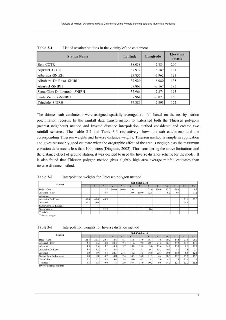
Table 3-1 List of weather stations in the vicinity of the catchment
Station Name Latitude Longitude Elevation (masl)
Beja-COTR 38.038 -7.884 206Aljustrel -COTR 37.972 -8.189 104Albernoa -SNIRH 37.857 -7.962 133Albufeira Do Roxo -SNIRH 37.929 -8.080 135Aljustrel -SNIRH 37.868 -8.167 193Santa Clara Do Louredo -SNIRH 37.966 -7.874 195Santa Victoria -SNIRH 37.964 -8.023 150Trindade -SNIRH 37.886 -7.893 172 The thirteen sub catchments were assigned spatially averaged rainfall based on the nearby station precipitation records. In the rainfall data transformation to watershed both the Thiessen polygons (nearest neighbour) method and Inverse distance interpolation method considered and created two rainfall schemes. The Table 3-2 and Table 3-3 respectively shows the sub catchments and the corresponding Thiessen weights and Inverse distance weights. Thiessen method is simple in application and gives reasonably good estimate when the orographic effect of the area is negligible as the maximum elevation deference is less than 100 meters (Dingman, 2002). Thus considering the above limitations and the distance effect of ground station, it was decided to used the Inverse distance scheme for the model. It is also found that Thiessen polygon method gives slightly high area average rainfall estimates than inverse distance method. Table 3-2 Interpolation weights for Thiessen polygon method
1 2 3 4 5 6 7 8 9 10 11 12 13Beja - Cotr 11.7 100.0 100.0 29.4 78.9 100.0 93.7 99.6 0.3Aljustrel - Cotr 16.5 70.6 100.0 12.8 6.3 0.4 77.5Albernoa Albufeira Do Roxo 50.0 67.0 49.9 25.9 22.3Aljustrel 50.1 33.0 74.1Santa Clara Do LouredoSanta Vitoria 21.9 8.4Trindade Thiessen weights
Station Sub Catchment
Table 3-3 Interpolation weights for Inverse distance method
1 2 3 4 5 6 7 8 9 10 11 12 13Beja - Cotr 22.4 21.3 20.1 2.6 8.3 13.8 17.0 16.1 7.5 10.2 14.6 21.6 20.7Aljustrel - Cotr 12.3 15.6 18.8 20.3 19.4 11.6 9.0 20.1 21.6 16.3 17.5 13.8 13.7Albernoa 9.9 6.3 5.2 14.5 13.7 15.8 15.8 9.0 12.6 14.9 13.0 8.0 11.9Albufeira Do Roxo 5.4 8.2 8.1 14.4 11.8 7.4 5.1 9.1 13.5 10.0 8.1 7.8 2.4Aljustrel 6.0 8.9 14.4 22.5 21.5 16.2 13.5 18.8 22.7 19.6 18.9 6.6 12.5Santa Clara Do Louredo 18.8 16.8 14.7 4.8 7.4 14.3 16.8 11.3 4.4 10.5 12.3 17.6 17.5Santa Vitoria 10.1 11.2 8.8 9.4 5.9 4.0 4.8 5.5 8.0 4.1 1.8 11.4 5.4Trindade 15.1 11.8 10.0 11.4 12.0 16.8 17.9 10.2 9.6 14.3 13.7 13.2 15.8Inverse distance weights
Station Sub Catchment

20
3.2.2. Evapotranspiration estimation
Evapotranspiration is one of the key inputs for the hydrologic model and it represents aggregated result of transporting water from the surface to the atmosphere. The reference crop evapotranspiration of the two near by COTR station data is based on the modified Penman-Monteith equation (Allen et al., 1998).
)34.01(
)(273
900)(408.0
2
2
u
eeuT
GRET
asn
o ++Δ
−+
+−Δ=
γ
γ [ 3.2]
Where ETo Reference crop evapotranspiration [mm day-1], Rn Net radiation at the crop surface [MJ m-2 day-1], G Soil heat flux density [MJ m-2 day-1], T Mean daily air temperature at 2 m height [°C], u2 Wind speed at 2 m height [m s-1], es Saturation vapour pressure [kPa], ea Actual vapour pressure [kPa], es - ea Saturation vapour pressure deficit [kPa], Δ Slope vapour pressure curve [kPa °C-1], γ Psychometric constant [kPa °C-1]. The reference crop evapotranspiration (ETo) daily time series data is available at the two COTR weather stations since September 2001 till to date. Further it was found that the ETo data of the two stations are homogeneous during the study period and had a good correlation among the reference crop evapotranspiration values. The Figure 3-4 depicts that two weather stations have almost the same
reference crop Evapotranspiration values. The coefficient of determination (R2) is almost equal to one showing excellent agreement, hence adoption of Thiessen polygon interpolation is considered reasonable. Thus, the spatial interpolation was carried out by the Thiessen polygon method in order to calculate ETo at sub catchment level.
Figure 3-4 Cumulative ETo comparison of the two COTR weather stations
Cummulative ETo Recorded at Beja and Aljustrel weather stations
y = 0.9582x - 53.129R2 = 0.9998
0
1000
2000
3000
4000
5000
6000
7000
8000
9000
10000
0 1000 2000 3000 4000 5000 6000 7000 8000 9000 10000
Cummulative ETo Beja (mm)
Cum
mul
ativ
e ET
o A
ljust
rel /
(mm
)
dd
Double mass relation
Linear (Double mass relation)

Analysis of Nutrient Dynamics in Roxo Catchment Using Remote Sensing data and Numerical Modeling
21
Table 3-4 Crop factors for different crop types
SunflowerWinter Wheat
Maize (sweet)
Growing-Olives Grapes Olives Bare Soils
Forests- Coniferous
Grazing Pasture
Kc ini 0.45 0.7 0.45 0.65 0.3 0.65 0.45 1 0.3Kc mid 1.15 1.15 1.15 0.7 0.7 0.45 0.45 1 0.75Kc end 0.35 0.25 1.05 0.7 0.45 0.65 0.45 1 0.75Max Crop height/(m) 2 1 1.5 3 to 5 1.5-2 10 0.1Source FAO 56
Crop Type
Stage
Table 3-5 Growing stages (days)
Crop Type Init.(Lini) Dev.(Ldev) Mid.(Lmid) Late.(Llate) Total Planting Date
Sunflower 25 35 45 25 130 AprilWinter Wheat 30 140 40 30 240 NovemberMaize (sweet) 20 25 25 10 80 May/JuneGrowing-Olives 30 90 60 90 270 MarchGrapes 30 60 40 80 210 AprilOlives 30 90 60 90 270 March
Source FAO 56
Daily area average crop coefficient plot for the catchment #01
0.500
0.550
0.600
0.650
0.700
0.750
0.800
0.850
0.900
0.950
J J F M A M J J A S O N D
Period
Res
ulta
nt K
c Fa
ctor
Catchment 1_ Resultant Kc Value
Figure 3-5 Weighted crop factors (Kc) for catchment #01
occ ETKET = [ 3.3]
Where: ETc Crop Evapotranspiration Kc Crop factor The basic information needed for estimation of crop evapotranspiration (ETc) had been collected from the FAO 56, Irrigation and Drainage paper and the data is summarised in Appendix 6. A GIS analysis was carried out to assess the different fractions of land use types within each sub-catchment.
22
During non growing periods surface is usually similar to bare soil and Allen et al (1998) recommends to use the Kc value equivalent to Kc,initial for non growing time periods. Accordingly weighted Kc factors were calculated considering the crop types, growth stage and individual crop factors, growing periods, etc. in a sub catchment. The area average (weighted) crop factors at daily time step were estimated for individual sub catchments. The weighted Kc variation for a period of one year in sub-catchment #01 is shown in the Figure 3-5, similarly for all other sub-catchments weighted Kc values were calculated for the estimation of crop evapotranspiration based on the equation [3.3].
3.3. Data preparation for reservoir water balance
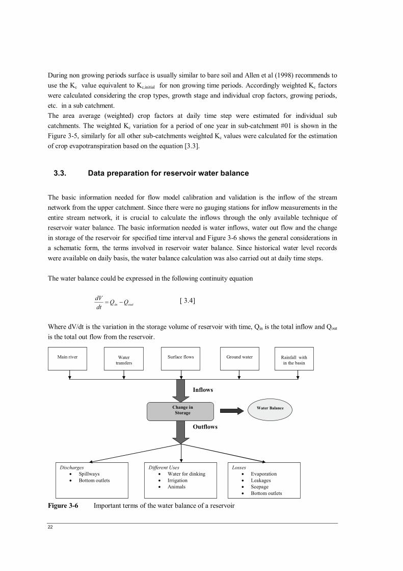
The basic information needed for flow model calibration and validation is the inflow of the stream network from the upper catchment. Since there were no gauging stations for inflow measurements in the entire stream network, it is crucial to calculate the inflows through the only available technique of reservoir water balance. The basic information needed is water inflows, water out flow and the change in storage of the reservoir for specified time interval and Figure 3-6 shows the general considerations in a schematic form, the terms involved in reservoir water balance. Since historical water level records were available on daily basis, the water balance calculation was also carried out at daily time steps. The water balance could be expressed in the following continuity equation
outin QQdtdV
−= [ 3.4]
Where dV/dt is the variation in the storage volume of reservoir with time, Qin is the total inflow and Qout
is the total out flow from the reservoir.
Surface flows
Water
transfers
Ground water
Inflows
Change in Storage
Outflows
Discharges • Spillways • Bottom outlets
Different Uses • Water for dinking • Irrigation • Animals
Losses • Evaporation • Leakages • Seepage • Bottom outlets
Water Balance
Main river
Rainfall with in the basin
Figure 3-6 Important terms of the water balance of a reservoir

Analysis of Nutrient Dynamics in Roxo Catchment Using Remote Sensing data and Numerical Modeling
23
3.3.1. Inflow
As displayed in the Figure 3-6 basic inflow to a reservoir could be listed as follows Qriver ; water flow in through the main river and tributaries, Qtran ; water flow accumulated through tributaries or trans-boundary flows, Qsurface ; surface flows due to rain events (overland flows directly comes in to reservoir. Qgf ; ground water flow comes in to the reservoir and Qrain ; water comes in due to rain events directly over the reservoir. Qin = Qriver + Qtran + Qsurface + Qgf + Qrain [ 3.5]
It is assumed that ground water flow in to the reservoir is very much equal to the ground water flow out hence Qgf term could be neglected in the final equation. So far there aren’t any trans-boundary flow in or out from the Roxo catchment and we can delete the term Qtran from the equation as well. Rain water come in (Qrain) can be assessed by the rainfall records from Albufeira Roxo floating rain gauge station. The only unknown parameter of the above equation [3.5] is Qriver and the main purpose of performing the water balance is to assess this parameter.
3.3.2. Outflow
The main outflows from the reservoir are discussed below Q uses ; discharge to various uses , drinking water supplies, Irrigation , and commercial purposes, Q operations ; discharges made under reservoir controls, spillway and bottom out let releases during flooding conditions, Q evp ; losses due to water surface evaporation from the reservoir water body, Q seepage ; seepage losses from the reservoir bed, The general equation for Qout could be written as follows Qout = Q uses + Q operations + Q evp + Q seepage [ 3.6] It is assumed that water loss as seepage is negligible due to relatively impervious nature of the reservoir bed, its acceptable as the reservoir sites are generally located in locations where there is relatively impervious soils. In addition with time bed become even more impervious due to the deposition of fine particles making it further water tight. This assumption was also affirmed by the ABROXO technical department where they stated no evidence of water loss observed as seepage. Further during the field visit we inspected the down stream of the reservoir and did not observe any dampness confirming our assumption.
3.3.3. Estimation of rainfall & evaporation volumes
The regular monitoring information available about the reservoir is the daily water levels at 1 cm precision. In estimation of daily water balances, the key information needed are water comes as direct precipitation on to the surface and water loss as evaporation from the surface. The water level in a reservoir relates to surface area with the stage area relationship and utilising this relationship it is possible to estimate water exchange quantities from the reservoir surface. Following section discuss about the stage area relationship of the Roxo reservoir.
24
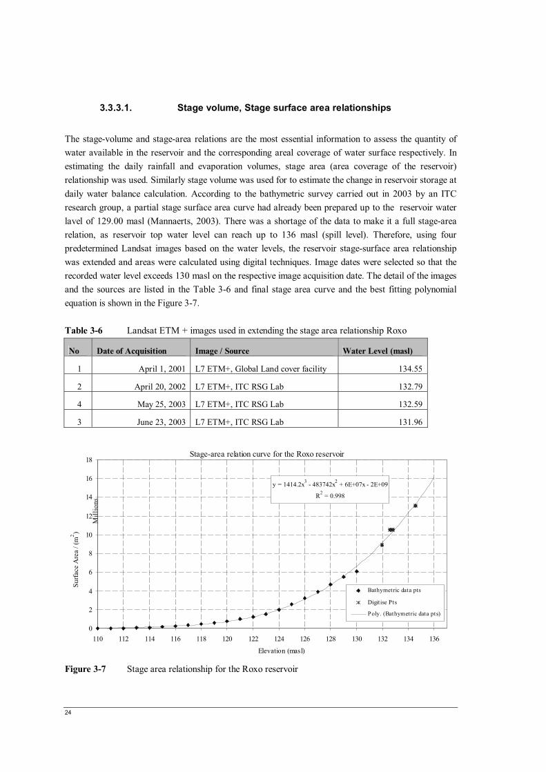
3.3.3.1. Stage volume, Stage surface area relationships
The stage-volume and stage-area relations are the most essential information to assess the quantity of water available in the reservoir and the corresponding areal coverage of water surface respectively. In estimating the daily rainfall and evaporation volumes, stage area (area coverage of the reservoir) relationship was used. Similarly stage volume was used for to estimate the change in reservoir storage at daily water balance calculation. According to the bathymetric survey carried out in 2003 by an ITC research group, a partial stage surface area curve had already been prepared up to the reservoir water lavel of 129.00 masl (Mannaerts, 2003). There was a shortage of the data to make it a full stage-area relation, as reservoir top water level can reach up to 136 masl (spill level). Therefore, using four predetermined Landsat images based on the water levels, the reservoir stage-surface area relationship was extended and areas were calculated using digital techniques. Image dates were selected so that the recorded water level exceeds 130 masl on the respective image acquisition date. The detail of the images and the sources are listed in the Table 3-6 and final stage area curve and the best fitting polynomial equation is shown in the Figure 3-7. Table 3-6 Landsat ETM + images used in extending the stage area relationship Roxo
No Date of Acquisition Image / Source Water Level (masl)
1 April 1, 2001 L7 ETM+, Global Land cover facility 134.55
2 April 20, 2002 L7 ETM+, ITC RSG Lab 132.79
4 May 25, 2003 L7 ETM+, ITC RSG Lab 132.59
3 June 23, 2003 L7 ETM+, ITC RSG Lab 131.96
Stage-area relation curve for the Roxo reservoir
y = 1414.2x3 - 483742x2 + 6E+07x - 2E+09
R2 = 0.998
0
2
4
6
8
10
12
14
16
18
110 112 114 116 118 120 122 124 126 128 130 132 134 136
Mill
ions
Elevation (masl)
Surfa
ce A
rea
/ (m
2 )
b
bb
Bathymetric data pts
Digitise Pts
Poly. (Bathymetric data pts)
Figure 3-7 Stage area relationship for the Roxo reservoir

Analysis of Nutrient Dynamics in Roxo Catchment Using Remote Sensing data and Numerical Modeling
25
Its it seen by Figure 3-7 that the new digitize points continue with the trend of the initial data set based on the bathymetric survey and the coefficient of determination [R2] value is very close to 1 indicating model predicts the stage surface area relation quite well with the data points. The stage-volume relation for the Roxo reservoir is already formulated by Mannaerts (2006) and it had been used in calculating the daily changes in storage based on daily water level changes and is shown in the Appendix 7.
3.3.3.2. Water surface evaporation
The evaporation from the free water surface is an important term in water balance calculation. The accuracy of the water balance calculation would consequently lead to an increase in reliability of the other terms of the water balance calculation. There are different possible ways in estimation of the water evaporation on the basis of data availability (Ali et al., 2008). According to SNIRH data base there were two stations close to Roxo reservoir (Barragem and Albufeira) and The Barragem station is already extinct and the Albufeira floating station shown Figure 3-8 is still under operation.
Figure 3-8 Albufeira Do Roxo floating station Table 3-7 Details of the weather stations located close to Roxo reservoir Barragem Do Roxo Albufeira Do Roxo Duration 1958-07-31 to 2001-03-31 2001–04-01 to current Location (lat, lon) 37.934296 N, 8.083004 W 37.928975 N, 8079641 W Status Extinct Active ET Method Class A Pan Evaporation Penman
Water surface evaporation estimation from the reservoir surface prior to April, 2001 was based on the Pan evaporation and used the following simple equation.
pco EKE = [ 3.7]
Where; Kc Pan coefficient Ep Pan Evaporation Eo Potential water surface evaporation
26
The Albufeira station has essential information that could be used for calculating the potential water surface evaporation. However since station does not have all the essential parameters measured, it was not possible to adopt the original Penman water surface evaporation equation, but the simplified method proposed by Valiantzas (2006) has been used for water surface evaporation. The accurate approximate version for Penman of Valiantzas (2006) is shown in the equation [3.8] below. The sample calculation sheet for the potential water surface evaporation is attached in the Appendix 3.
( ) ( )
( ) ( )uaRHT
RHTTxRR
TTRE
u
A
ssPEN
536.0100
13.16049.0
100463.07.000014.01194.013188.05.9)1(051.0
max
2minmax
+⎟⎠⎞
⎜⎝⎛ −++
⎟⎟⎠
⎞⎜⎜⎝
⎛++−⎟⎟
⎠
⎞⎜⎜⎝
⎛−−−+−= α [ 3.8]
Where
EPEN Potential water surface evaporation aU Wind function coefficient (1: for original penman equation) u Wind velocity in (m/s) RA Extraterrestrial radiation in (MJ/m2/d) RS Measure solar radiation at surface (MJ/m2/d) RH Relative humidity in (%). T Temperature in °C α Water surface albedo (0.08)
Valiantzas (2006) further stated that the accuracy of the above equation was tested for different countries and different climatic conditions and conclude that the above equation performs relatively good as the results were perfectly close and in agreement with the original penman water surface evaporation equation.
3.3.3.3. Direct rainfall (input)
Daily rainfall data observed at the Albufeira do Roxo floating station have been used to calculate the rain water falling directly on the reservoir surface since 2001 to 2008, while the Barragem do Roxo station data have been used for same calculations prior to that period. There were few data gaps and those were filled considering the regression analysis performed with the nearby Beja (COTR) weather station as it was found a reasonably good correlation with the two stations as shown in the Figure 3-9. Finally the volume of water comes on to the reservoir surface as direct precipitation was estimated using the stage area relationship at daily time steps.
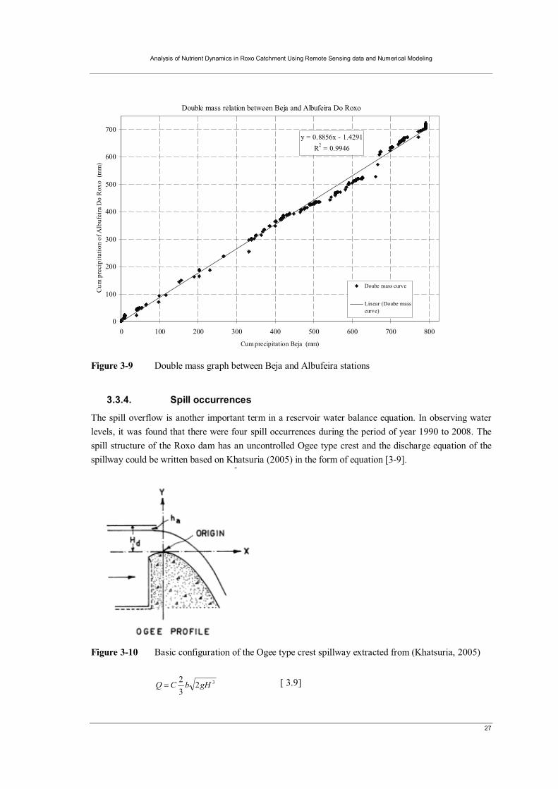
Analysis of Nutrient Dynamics in Roxo Catchment Using Remote Sensing data and Numerical Modeling
27
Double mass relation between Beja and Albufeira Do Roxo
y = 0.8856x - 1.4291R2 = 0.9946
0
100
200
300
400
500
600
700
0 100 200 300 400 500 600 700 800
Cum precipitation Beja (mm) jjj
Cum
pre
cipi
tatio
n of
Alb
ufei
ra D
o R
oxo
(mm
)
jjj
Doube mass curve
Linear (Doube masscurve)
Figure 3-9 Double mass graph between Beja and Albufeira stations
3.3.4. Spill occurrences
The spill overflow is another important term in a reservoir water balance equation. In observing water levels, it was found that there were four spill occurrences during the period of year 1990 to 2008. The spill structure of the Roxo dam has an uncontrolled Ogee type crest and the discharge equation of the spillway could be written based on Khatsuria (2005) in the form of equation [3-9].
Figure 3-10 Basic configuration of the Ogee type crest spillway extracted from (Khatsuria, 2005)
3232 gHbCQ = [ 3.9]
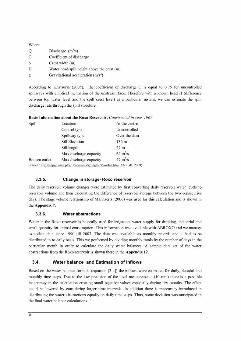
28
Where Q Discharge (m3/s) C Coefficient of discharge b Crest width (m) H Water head/spill height above the crest (m) g Gravitational acceleration (m/s2) According to Khatsuria (2005), the coefficient of discharge C is equal to 0.75 for uncontrolled spillways with elliptical inclination of the upstream face. Therefore with a known head H (difference between top water level and the spill crest level) at a particular instant, we can estimate the spill discharge rate through the spill structure. Basic Information about the Roxo Reservoir: Constructed in year 1967 Spill Location At the centre Control type Uncontrolled Spillway type Over the dam Sill Elevation 136 m Sill length 27 m Max discharge capacity 64 m3/s Bottom outlet Max discharge capacity 47 m3/s Source : http://cnpgb.inag.pt/gr_barragens/gbingles/RoxoIng.htm (CNPGB, 2009)
3.3.5. Change in storage- Roxo reservoir
The daily reservoir volume changes were estimated by first converting daily reservoir water levels to reservoir volume and then calculating the difference of reservoir storage between the two consecutive days. The stage volume relationship of Mannaerts (2006) was used for this calculation and is shown in the Appendix 7.
3.3.6. Water abstractions
Water in the Roxo reservoir is basically used for irrigation, water supply for drinking, industrial and small quantity for animal consumption. This information was available with ABROXO and we manage to collect data since 1990 till 2007. The data was available as monthly records and it had to be distributed in to daily basis. This we performed by dividing monthly totals by the number of days in the particular month in order to calculate the daily water balances. A sample data set of the water abstractions from the Roxo reservoir is shown there in the Appendix 12.
3.4. Water balance and Estimation of inflows
Based on the water balance formula (equation [3-4]) the inflows were estimated for daily, decadal and monthly time steps. Due to the low precision of the level measurements (10 mm) there is a possible inaccuracy in the calculation creating small negative values especially during dry months. The effect could be lowered by considering larger time intervals. In addition there is inaccuracy introduced in distributing the water abstractions equally on daily time steps. Thus, some deviation was anticipated in the final water balance calculations.
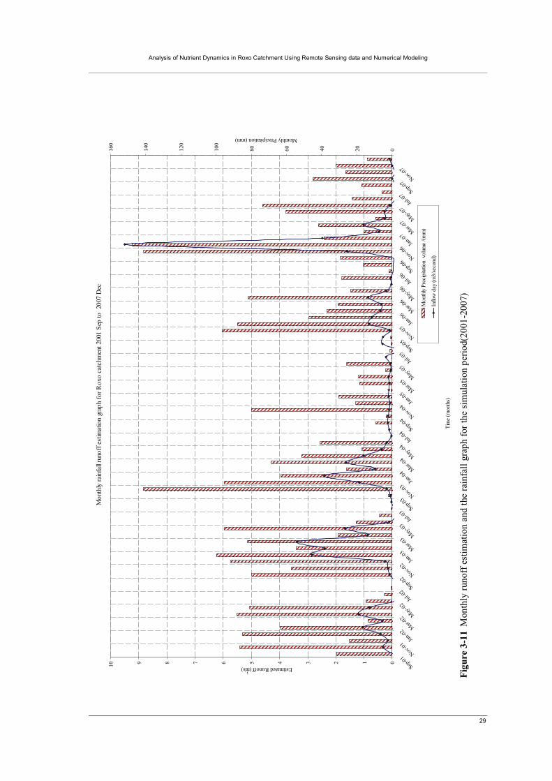
Analysis of Nutrient Dynamics in Roxo Catchment Using Remote Sensing data and Numerical Modeling
29
Fi
gure
3-1
1 M
onth
ly ru
noff
estim
atio
n an
d th
e ra
infa
ll gr
aph
for t
he s
imul
atio
n pe
riod(
2001
-200
7)
Mon
thly
rain
fall
runo
ff es
timat
ion
grap
h fo
r Rox
o ca
tchm
ent 2
001
Sep
to 2
007
Dec
012345678910 Sep-01
Nov-01
Jan-02
Mar-02
May-02
Jul-02
Sep-02
Nov-02
Jan-03
Mar-03
May-03
Jul-03
Sep-03
Nov-03
Jan-04
Mar-04
May-04
Jul-04
Sep-04
Nov-04
Jan-05
Mar-05
May-05
Jul-05
Sep-05
Nov-05
Jan-06
Mar-06
May-06
Jul-06
Sep-06
Nov-06
Jan-07
Mar-07
May-07
Jul-07
Sep-07
Nov-07
Tim
e (m
onth
s)
Estimated Runoff (m3/s) jjjj
020406080100
120
140
160
Monthly Precipitation (mm) jjj
Mon
thly
Prec
ipita
tion
vol
ume
/(mm
)
Inflo
w d
ay (m
3/se
cond
)

30
The runoff values were estimated for the time period starting from January 1990 to December 2007. In order to perform model calibration and validation, decadal runoff data have been used since September 2001. The monthly runoff hydrograph for the simulation period is shown in Figure 3-11 and it shows the inflows are having few peaks after strong rainfall incidents and during the dry months the inflow are very minimal or almost zero. The Appendix 16 illustrates the sample water balance calculation excel sheet and the estimated decadal runoff hydrograph for the Roxo reservoir.
3.5. Water quality data
Water quality data is important information in the subsequent modeling work, therefore water samples were collected at suitable locations of the streams and Figure 2-1 shows the exact locations. The sample collection and analysis were carried out according to the guidelines set by the standard reference text books at ITC (Chapman, 1996), (Dost, 2006). Before going to field work, the sample collection bottles (HDPE) were cleaned with 1%-3% Nitric acid for 24 hours and consequently rinsed with distilled water. At each sampling point, key information on the particular location were noted down, the date, time, GPS coordinates, water colour, possible contaminants, flow condition, surrounding land cover, were among the recorded information. The water samples were collected on the 10th Oct 2008 so that samples remained a minimum time at Beja before returning back to ITC. Seven water samples were collected along the Chamine River and one from the Roxo reservoir. There were low water flows occurring in the stream and mostly the width of the water flow was less than 2 m and depth of the flow was about 2-10 cm depending on the location. The effort had been made to take water sample without disturbing the bed sediments. Generally the samples were taken close to the top and at the centre of the flow section. The samples were filtered with disposable syringe mounted 0.45 micron Whatman filters and two samples bottles were collected from each site, one having 200 ml of water sample acidified with HNO3 while the second sample has 100 ml of sample water acidified with HCl. The sample bottles were filled up to the top and caps were properly tightened so that no interaction with air. Each sample bottle was named giving the date, time, location ID and the acid type used as preservative. As soon as the samples were brought to the shelter care had been taken to keep them inside the cooler (below 4oC).
3.5.1. In-situ water tests
The temperature, electrical conductivity (EC), pH and alkalinity tests were carried out at the sampling location and the HACH HQ 40D multi probe device was used to measure temperature and EC. Prior to taking the measurements the sensor probe was calibrated with the standard solution provided with the equipment. An alkalinity test kit was used to test the alkalinity. The in situ test results are show in the Table 3-8.
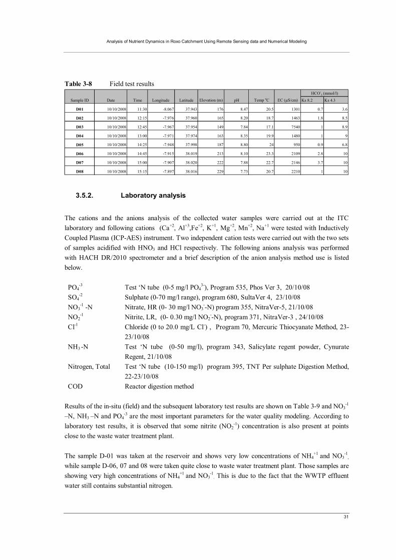
Analysis of Nutrient Dynamics in Roxo Catchment Using Remote Sensing data and Numerical Modeling
31
Table 3-8 Field test results
Ks 8.2 Ks 4.3
D01 10/10/2008 11:30 -8.067 37.943 176 8.47 20.5 1301 0.7 3.6
D02 10/10/2008 12:15 -7.976 37.960 165 8.20 18.7 1463 1.8 8.5
D03 10/10/2008 12:45 -7.967 37.954 149 7.84 17.1 7540 1 8.9
D04 10/10/2008 13:00 -7.971 37.974 163 8.35 19.9 1480 1 9
D05 10/10/2008 14:25 -7.948 37.998 187 8.80 24 950 0.9 6.8
D06 10/10/2008 14:45 -7.915 38.019 213 8.10 23.3 2109 2.8 10
D07 10/10/2008 15:00 -7.907 38.020 222 7.88 22.7 2146 3.7 10
D08 10/10/2008 15:15 -7.897 38.016 229 7.73 20.7 2210 1 10
pH Temp oC EC (μS/cm)HCO-
3 (mmol/l)
Longitude Latitude Elevation (m)Sample ID Date Time
3.5.2. Laboratory analysis
The cations and the anions analysis of the collected water samples were carried out at the ITC laboratory and following cations (Ca+2, Al+3,Fe+2, K+1, Mg+2, Mn+2, Na+1 were tested with Inductively Coupled Plasma (ICP-AES) instrument. Two independent cation tests were carried out with the two sets of samples acidified with HNO3 and HCl respectively. The following anions analysis was performed with HACH DR/2010 spectrometer and a brief description of the anion analysis method use is listed below. PO4
-3 Test ‘N tube (0-5 mg/l PO43-), Program 535, Phos Ver 3, 20/10/08
SO4-2 Sulphate (0-70 mg/l range), program 680, SultaVer 4, 23/10/08
NO3-1 -N Nitrate, HR (0- 30 mg/l NO3
--N) program 355, NitraVer-5, 21/10/08 NO2
-1 Nitrite, LR, (0- 0.30 mg/l NO2--N), program 371, NitraVer-3 , 24/10/08
Cl-1 Chloride (0 to 20.0 mg/L Cl-) , Program 70, Mercuric Thiocyanate Method, 23-23/10/08
NH3 -N Test ‘N tube (0-50 mg/l), program 343, Salicylate regent powder, Cynurate Regent, 21/10/08
Nitrogen, Total Test ‘N tube (10-150 mg/l) program 395, TNT Per sulphate Digestion Method, 22-23/10/08
COD Reactor digestion method Results of the in-situ (field) and the subsequent laboratory test results are shown on Table 3-9 and NO3
-1 –N, NH3 –N and PO4
-3 are the most important parameters for the water quality modeling. According to laboratory test results, it is observed that some nitrite (NO2
-1) concentration is also present at points close to the waste water treatment plant. The sample D-01 was taken at the reservoir and shows very low concentrations of NH4
+1 and NO3
-1,
while sample D-06, 07 and 08 were taken quite close to waste water treatment plant. Those samples are showing very high concentrations of NH4
+1 and NO3
-1. This is due to the fact that the WWTP effluent
water still contains substantial nitrogen.
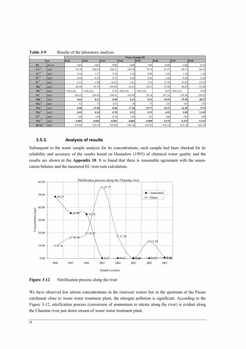
32
Table 3-9 Results of the laboratory analysis
D 01 D 02 D 03 D 04 D 05 D 06 D 07 D 08EC μS/cm 1301 1463 7540 1480 950 2109 2146 2210Ca+2 mg/l 64.38 104.62 520.31 105.98 78.79 91.97 88.71 88.65Al +3 mg/l 0.14 1.37 3.34 1.24 0.80 2.29 1.12 1.34Fe+2 mg/l 0.45 0.35 0.37 0.45 0.62 1.06 0.38 0.56K +1 mg/l 6.31 3.59 18.23 3.41 3.23 27.29 25.02 27.61Mg+2 mg/l 43.48 55.79 345.69 61.41 39.27 47.68 46.43 47.42Mn+3 mg/l < Det.Lim < Det.Lim 0.36 < Det.Lim < Det.Lim 0.07 < Det.Lim 0.02Na+ mg/l 106.43 109.45 550.41 103.09 50.36 197.24 195.96 199.83
NH4 + mg/l 0.61 0.12 0.00 0.12 0.12 34.53 35.50 48.27
SO4-2 mg/l 62 75 625 70 75 125 135 135
NO3-1 mg/l 0.00 13.28 0.00 17.26 55.77 19.47 16.38 9.74
PO4-3 mg/l 0.03 0.24 0.78 0.21 0.33 6.55 9.85 11.65
Cl-1 mg/l 144 165 2130 236 125 446 392 390
NO2-1 mg/l 0.003 0.004 0.003 0.004 0.009 0.375 0.475 0.125
HCO3-1 mg/l 219.66 518.65 543.06 549.16 414.92 610.18 610.18 610.18
TestWater Sample ID
3.5.3. Analysis of results
Subsequent to the water sample analysis for its concentrations, each sample had been checked for its reliability and accuracy of the results based on Hounslow (1995) of chemical water quality and the results are shown in the Appendix 10. It is found that there is reasonable agreement with the anion-cation balance and the measured EC-iron sum calculation.
Nitrification process along the Chamine river
48.27
35.50 34.53
0.12 0.12 0.00 0.12 0.61
9.74
16.3819.47
55.77
17.26
0.00
13.28
0.000.00
10.00
20.00
30.00
40.00
50.00
60.00
D08 D07 D06 D05 D04 D03 D02 D01
Sample Location
Con
cent
ratio
n (m
g/l
AmmoniumNitrate
Figure 3-12 Nitrification process along the river We have observed low nitrate concentrations in the reservoir waters but in the upstream of the Pisoes catchment close to waste water treatment plant, the nitrogen pollution is significant. According to the Figure 3-12, nitrification process (conversion of ammonium to nitrate along the river) is evident along the Chamine river just down stream of waste water treatment plant.

Analysis of Nutrient Dynamics in Roxo Catchment Using Remote Sensing data and Numerical Modeling
33
3.6. Flow measurements
An estimation of stream flow of the Pisoes river was carried out at sampling point D_04 (37o,57’ 34.5” N, 7o 58’ 33.8” W). Due to time constraints, we could only manage to do a single flow measurement. The standard procedure listed in the Butterworth et al., (2000) was adopted for the salt dilution method. Some key information with respect to the salt dilution test is listed below. Salt - NaCl Applied Quantity (NaCl) - 400 g Distance of the stretch - 20 m (application of salt and subsequent EC measurement point) Instrument - HACH HQ 40D multi- probe device for EC measurements The primary objective of the dilution gauging is to make a realistic assessment over the stream flow rate of the selected stretch. The flow rate was estimated using the mass conservation during the advective and dispersive solute transport equation and it is listed below.
( )
( )( )∫∞
−=
0,1
tbtx
xo
CC
MQ [ 3.10]
Where M(xo) - Salt load applied at the application position [g] Q - Flow rate [m3/sec] C(x1,t) - Salt concentration at time “t” at the selected position [mg/l] Cb - Initial salt concentration [mg/l] The estimated stream flow at sample point D_04 is 0.12 m3/s and it is relatively similar to the initial quick guess made through the float at the selected position. The electrical conductivity (EC) measurements and other relevant information on the salt dilution gauging technique is listed Appendix 11.
3.7. Soil data
Soil data is key information needed in defining RAM surface properties in Duflow. The rainfall runoff elements (RAM) needs several parameters that are relevant to soil properties of the catchment. According to the soil map of the study area shown in Appendix 2_fig.(b), it is found that there are about 40 soil units present, but in modeling work we need to give and area-averaged parameter value for sub-catchment. The data of the soil properties of individual soil class were collected from the soil reference books (Cardoso, 1965), (Conference on Mediterranean Soils, 1966). According to the Portugal soil map, the major soil units present in the Roxo catchment and its percentages are listed in the Table 3-10.
34
Table 3-10 Major soil types in the Roxo catchment
Modern alluvial soil non calcareous A;A(h); Asoc 2.58%
Brown Calcareous Soils Brown Calc.S. of Sub-humic and semi arid climates Pc ;Pcx 1.14%
Red Calcareous Soils Red Calc.S. of Sub-Hum and Semi Arid Climates Vcx; Vc 10.71%
Non Calcareous Black Barros Bp 1.47%
Calcareous Black Barros Strongly decarbonated Bpc 8.16%
Calcareous Black Barros Slightly decarbonated Cp 1.40%
Brown Medit.S.from calcareous rocks Pac; 0.92%
Brown Medit.S.from non-calcareous rocks - Normals Px 13.68%
Brown Medit.S.from non-calcareous rocks - Para Hydromophic Pag 1.55%
Red-Yel. Medit.S.from non-calcarioos rocks - Normals Vx; Vx(d); Vx(d,p);Vx(p) 21.42%
Red-Yel. Medit.S.from non-calcareous rocks - with plinthitic materials Sr* 16.63%
With Eluvial Horizon Planosols with Eluvial Horison Ps 9.37%Hydromorphic Organic Soils Peaty Soils Peaty Soils Sp 1.61%
Percentage %Soil type I Soil type II Detailed classification type IV
Black Barros
Soils Lessives (Not Strongly Unsaturated)
Brown Mediterranean Soils
Red-Yellow Mediterranean Soils
Barros
Hydromorphic Soils
Calcareous Soils
Incipient Soils Alluvial Soils
Symbol
The Table 3-10 summarises that the high percentage of soils in the catchment belongs to Mediterranean soil types. The basic soil properties relevant in modeling work are porosity, moisture content at different pF values (saturation, field capacity and wilting point), initial and constant infiltration rates,. The relevant information extracted from the literature are summarised in the Appendix 8. This information is used as the initial estimate for setting up the model parameters for unpaved surfaces of the RAM elements. The Appendix 2_fig.(b) shows the composite soil map of the Roxo catchment.
3.8. Land cover data
Land cover-land use (LCLU) data is essential information required in hydraulic and water quality modeling. In defining a RAM element in Duflow for a selected basin, we have to categorise sub basin or RAM area in to open water, green houses, sewer, other-paved and unpaved surfaces then need to input the fractions of the land in each category as percentages. Thus, it was essential to have a detailed land cover information for the model building. It was decided to use CORINE land cover classification that have 44 detailed classes in the surface classification and it is comparatively easy to categorise areas according to the requirements of Duflow. The CORINE land-cover land-use is produced using Landsat 7 ETM + sensor and is available in vector data format with minimum mapping units of 25 hectares (Caetano and Araújo, 2006) and also is having an overall thematic accuracy beyond 82 % (Caetano et al., 2006). The land cover map of the area is given in the Appendix 2_fig.(a) and during the field visit we have collected information for an accuracy assessment. It was found that the overall accuracy is very close to 90%. Thus, CORINE LCLU was judged a reasonable data set for the surface classification according to the model requirements. The land cover classes had been re-categorised as presented in the Table 3-11.
Analysis of Nutrient Dynamics in Roxo Catchment Using Remote Sensing data and Numerical Modeling
35
Table 3-11 Reclassification of CORINE land cover classes to DUFLOW RAM
Code CLC_Level 1 CLC_Level 2 CLC_Level 3 Re classification
112 Artificial surfaces Urban fabric Discontinuous urban fabric Other paved
211 Agricultural areas Arable land Non-irrigated arable land Unpaved
212 Agricultural areas Arable land Permanently irrigated land Unpaved
221 Agricultural areas Permanent crops Vineyards Unpaved
223 Agricultural areas Permanent crops Olive groves Unpaved
241 Agricultural areas Heterogeneous agricultural areas Annual crops associated with permanent crops Unpaved
242 Agricultural areas Heterogeneous agricultural areas Complex cultivation patterns Unpaved
243 Agricultural areas Heterogeneous agricultural areas Land principally occupied by agriculture, with significant areas of natural vegetation Unpaved
244 Agricultural areas Heterogeneous agricultural areas Agro-forestry areas Unpaved
311 Forest and semi natural areas Forests Broad-leaved forest Unpaved
313 Forest and semi natural areas Forests Mixed forest Unpaved
321 Forest and semi natural areasScrub and/or herbaceous vegetation associations Natural grasslands Unpaved
324 Forest and semi natural areasScrub and/or herbaceous vegetation associations Transitional woodland-shrub Unpaved
512 Water bodies Inland waters Water bodies Open Water
In the Roxo catchment land cover fractions, falling under the definition of sewered areas and green-house were considered negligible based on the CORINE land-cover classification. During the field visits also we did not observe land use that comes under above categories. The land cover information was further used in the estimation of crop evapotranspiration. The procedure followed in estimation of crop evapotranspiration was discussed in chapter 3.2.2 in detail.
3.9. Historical water qauality data
Historical water quality data is obligatory for the water quality model assessment in its prediction. Generally it’s difficult to find continuous time series of water quality data and the condition is same for Roxo catchment. Few past water quality test records have been collected from the EMAS. The EMAS data refers to the water quality tests performed at their intake of the reservoir. Test data was available since Jan 2005 to Jan 2008 at monthly time steps and is show in the Appendix 14.1. In addition, some of the previous ITC’s research MSc were focused on water quality in the Roxo catchment that also provides information on water quality in the Roxo stream network (Awino, 2003). This information is summarized in the Appendix 14.2.

36

Analysis of Nutrient Dynamics in Roxo Catchment Using Remote Sensing data and Numerical Modeling
37
4. Numerical Modeling
4.1. Duflow Modeling Studio (DMS)
DUFLOW is a software package for simulating one-dimensional steady, unsteady flow in open-channel systems One can acquire it for a relatively low cost (Clemmens et al., 1993). Duflow facilitates dynamic management of water systems, with for example, applications in diverse areas like agriculture, water supply, fisheries, energy and water quality control (DUFLOW, 2004a). The program is provided with a graphical user interface (GUI) thus, it is interactive and reasonably fast in learning. The programme is frequently used by the water authorities, designing hydraulic structures and for teaching/academic purposes. The DMS program is designed for simple networks of channels with simple structures. The result of a modeling can be displayed in time and space for immediate analysis. The Duflow Modeling Studio consists of following key features;
1. Duflow water quantity model Used for unsteady flow calculation in streams and rivers
2. Duflow water quality model Simulation complex water quality processes in the streams and water bodies
3. RAM precipitation runoff module Used for modeling rainfall runoff processes from land areas
4. MODUFLOW This program is used to link the Duflow model with MODFLOW (ground water model)
In this research, first three tools in DMS listed above have been used and the results of the RAM calculations are used as input boundary calculation to the DUFLOW calculation.
4.2. Duflow flow model
The water levels and flow rates are determined by solving the Saint Venant’s equations of continuity and momentum using the four point implicit Preissmann numerical scheme. The basic 1-D equations used in the model are listed as follows;
oxQ
tB
=∂∂
+∂∂
[ 4.1] Continuity equation
( ) ( )φγνα−Φ=+
∂∂
+∂∂
+∂∂ cos2
2 waARCQQg
xQ
xHgA
tQ [ 4.2] Momentum equation

38
Where; t Time [s] x Distance as measured along the channel axis [m] H(x, t) Water level with respect to reference level [m] v(x, t) Mean velocity (averaged over the cross-sectional area) [m/s] Q(x, t) Discharge at location x and at time t [m3/s] R(x, H) Hydraulic radius of cross-section [m] a(x, H) Cross-sectional flow width [m] A(x, H) Cross-sectional flow area [m2] b(x, H) Cross-sectional storage width [m] B(x, H) Due to gravity [m/s2] C(x, H) Coefficient of De Chézy [m1/2/s] w(t) Wind velocity [m/s] Φ(t) Wind direction in degrees [degrees] f(x) Direction of channel axis in degrees, measured clockwise from the north [degrees] γ(x) Wind conversion coefficient [-] α Correction factor for non-uniformity of the velocity distribution in the advection term After solving the above equations [4-1, 4-2] using the 4 point Preissmann scheme, each channel of the network will have 2 equations with unknown Q and H for the new time level. For the unique solution of the set of equations, the additional conditions have to be specified at boundaries of the network and at the sections defined as structures. These boundary conditions are in the form of heads (H), discharges (Q) or combination of both (Q-H).
4.3. Duflow quality model
Duflow quality model is based on the one dimensional transport equation listed as equation [4.3] and this partial differential equation is used to describe concentration of constituents at space and time in 1-D flow system.
( ) ( ) PxCAD
xxQC
tBC
+⎟⎠⎞
⎜⎝⎛
∂∂
∂∂
+∂
∂−=
∂∂ [ 4.3]
where: C Constituent concentration [g/m3] Q Flow [m3/s] A Cross-sectional flow area [m2 ] D Dispersion coefficient [m2 /s] B Cross-sectional storage area [m2 ] x x-coordinate [m] t Time [s] P Production of the constituent per unit length of the section [g/ms]
Analysis of Nutrient Dynamics in Roxo Catchment Using Remote Sensing data and Numerical Modeling
39
The general advection-diffusion/dispersion processes are represented in the first two terms of the right hand side of the equation 4-3. The production term listed in equation (P) represent all the physical, chemical and biological processes that undergo by a particular constituent. The user has the freedom of defining the processes (Windemuller et al., 1997). This model/ process description file can be created and edited in the user interface and later complied with the DUPROL. During this compilation stage the process descriptions are converted in to readable format of the programming part of Duflow (DUFLOW, 2004a). Finally, these process descriptions are coupled with the transport equation to produce a numerical solution. The model has to be provided with initial and boundary condition to run for all state variables (concentrations). The initial conditions are provided to all nodes and the initial conditions are based on historical records, best approximate guesses or by using the results of the former computations. The boundary conditions are provided at the physical boundaries of the system or at the internal boundaries. The boundary conditions can be provided either as concentrations or loads for quality model.
4.4. Duflow rainfall runoff (RAM) component
The rainfall runoff modeling component describes the processes in the hydrologic cycle that occur at the land surface after incidental precipitation with the discharge as a runoff to the ground water or the surface water. In order to describe rainfall runoff processes with RAM, the evaporation, precipitation intensity, soil and terrain properties of the catchment or land area are essential input information. The soil information includes actual, maximum and minimum moisture contents, infiltration rates, depth to the water table, etc are also essential in describing the processes. In RAM, the rainfall runoff processes is described at land area i.e. catchment level and uses a conceptual rainfall runoff (linear reservoir) model rather than a physical-mathematical model. The framework of the precipitation runoff model is shown in the Figure 4-1 and it was extracted from the Duflow manual (DUFLOW, 2004b).
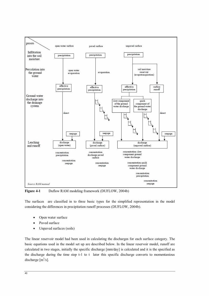
40
Figure 4-1 Duflow RAM modeling framework (DUFLOW, 2004b) The surfaces are classified in to three basic types for the simplified representation in the model considering the differences in precipitation runoff processes (DUFLOW, 2004b).
• Open water surface • Paved surface • Unpaved surfaces (soils)
The linear reservoir model had been used in calculating the discharges for each surface category. The basic equations used in the model set up are described below. In the linear reservoir model, runoff are calculated in two stages, initially the specific discharge [mm/day] is calculated and it is the specified as the discharge during the time step t-1 to t later this specific discharge converts to momentanious discharge [m3/s].
Source RAM manual

Analysis of Nutrient Dynamics in Roxo Catchment Using Remote Sensing data and Numerical Modeling
41
4.4.1. Open water surface
The water bodies like reservoirs, rivers and lakes in a catchment considered under the surface category of open water bodies, and water loss only by means of evaporation and generally there aren’t any delays in runoff generation from the open water surfaces.
trotbtwateropenN EfPP ,,,_, −= [ 4.4]
⎟⎠⎞
⎜⎝⎛ −+=
Δ−Δ−
−oo k
t
twateropenNk
t
twateropentwateropen ePeqq 1,_,1,_,_ [ 4.5]
twateropentwateropentwateropen qaAQ ,_,_,_ = [ 4.6]
Where; Input Pb,t [mm/day] Precipitation intensity Er,t [mm/day] Reference crop evaporation Makkink qopen_water,t-1 [mm/day] Specific discharge open water surface Aopen_water [ha] Open water surface Model parameters f0 [-] Crop factor Makkink for open water
k0 [day] Time constant reservoir open water surface Δt [day] Time step a [-] Conversion factor units
Output PN,open_water,t [mm/day] Effective precipitation open water surface Qopen_water,t [m3/s] Discharge open water surface
4.4.2. Paved surface
The paved areas are further divided in to 3 categories as paved rural, urban and green houses. Discharge from the paved surface can occur by means of (a) paved surface discharge directly through the drainage system, (b) surface discharge by mean of separated sewer systems or (c) surface covered with green house. However in the study area there were very limited paved surface area and all belongs categorized under the 1st category (paved surface discharge directly through the drainage system). The governing equations [4.5] are listed below.

42
tB
EfPI totrotbto Δ
+−= −1,,,,
[ 4.7]
tB
It
BEfPP v
toto
trotbtoN Δ−−
Δ+−= − max,
,1,
,,,, [ 4.8]
⎟⎠⎞
⎜⎝⎛ −+=
Δ−Δ−
−oooo k
t
toNk
t
tootoo ePeqq 1,,1,,,, [ 4.9]
tooootoo qaAQ ,,,,, = [ 4.10]
⎟⎠⎞
⎜⎝⎛ −+=
Δ−Δ−
−oioi k
t
tok
t
tiotio eIeqq 1,1,,,, [ 4.11]
( )oorotiotio AAaqQ ,,,,,, −= [ 4.12]
Where Input Pb,t [mm/day] precipitation intensity Bo,t-1 [mm] storage at open paved surface Er,t [mm/day] reference crop evaporation Makkink qo,o,t-1 [mm/day] specific discharge other open paved surface (formula Ao,o [ha] other open paved surface
qo,i,t-1 [mm/day] specific discharge infiltrated water Ii,o [mm/day] infiltration intensity open paved surface Ao,r [ha] open paved surface with sewer system Model parameters Io,max [mm] infiltration capacity fo [-] crop factor Makkink open water Δt [day] Time step Bv,max [mm] maximum storage at surface ko,o [day] time constant reservoir other open paved surface ki [day] time constant reservoir a [-] Factor output Io,t [mm/day] infiltration intensity PN,o,t [mm/day] surface runoff at open paved surface
qo,o,t-1 [mm/day] specific discharge other open paved surface Qo,o,t [m3/s] discharge from other open paved surface
qo,i,t-1 [mm/day] specific discharge infiltrated water Qo,i,t [m3/s] discharge infiltrated water from open paved surface
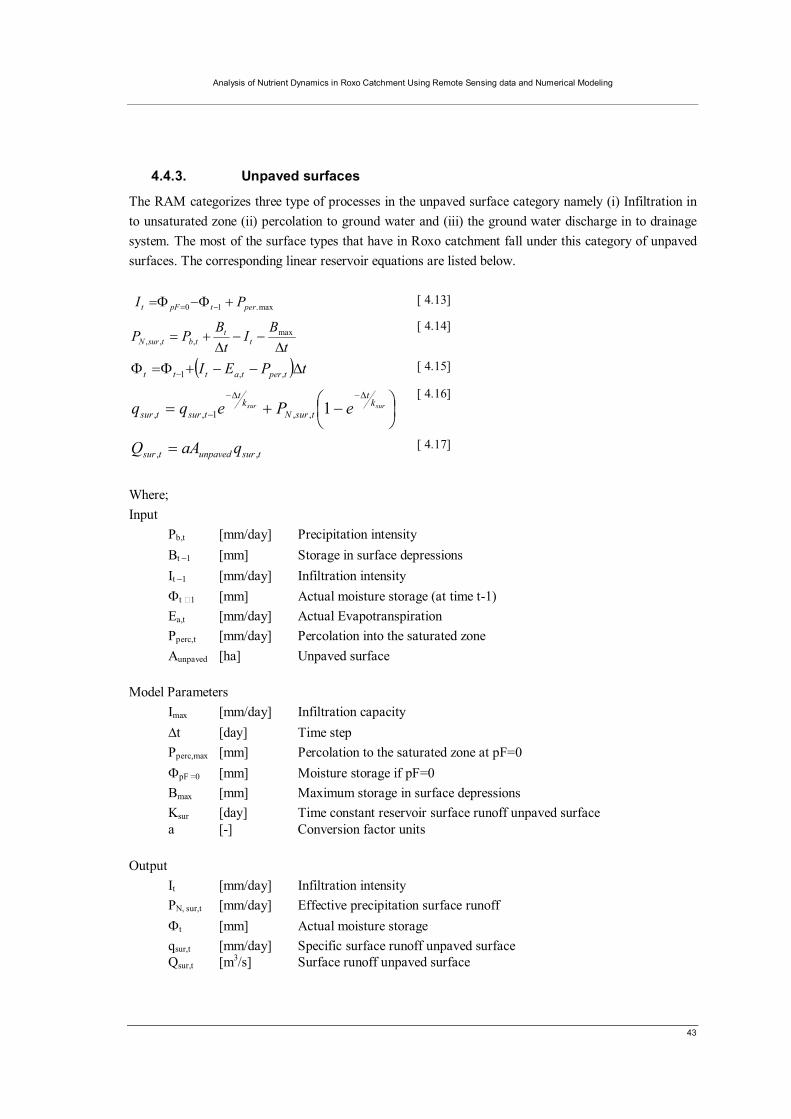
Analysis of Nutrient Dynamics in Roxo Catchment Using Remote Sensing data and Numerical Modeling
43
4.4.3. Unpaved surfaces
The RAM categorizes three type of processes in the unpaved surface category namely (i) Infiltration in to unsaturated zone (ii) percolation to ground water and (iii) the ground water discharge in to drainage system. The most of the surface types that have in Roxo catchment fall under this category of unpaved surfaces. The corresponding linear reservoir equations are listed below. max.10 pertpFt PI +Φ−Φ= −= [ 4.13]
tBI
tBPP t
ttbtsurN Δ
−−Δ
+= max,,,
[ 4.14]
( ) tPEI tpertattt Δ−−+Φ=Φ − ,,1 [ 4.15]
⎟⎠⎞
⎜⎝⎛ −+=
Δ−Δ−
−sursur k
t
tsurNk
t
tsurtsur ePeqq 1,,1,, [ 4.16]
tsurunpavedtsur qaAQ ,, = [ 4.17]
Where; Input Pb,t [mm/day] Precipitation intensity Bt −1 [mm] Storage in surface depressions It −1 [mm/day] Infiltration intensity Φt �1 [mm] Actual moisture storage (at time t-1) Ea,t [mm/day] Actual Evapotranspiration Pperc,t [mm/day] Percolation into the saturated zone Aunpaved [ha] Unpaved surface Model Parameters Imax [mm/day] Infiltration capacity Δt [day] Time step Pperc,max [mm] Percolation to the saturated zone at pF=0 ΦpF =0 [mm] Moisture storage if pF=0 Bmax [mm] Maximum storage in surface depressions Ksur [day] Time constant reservoir surface runoff unpaved surface a [-] Conversion factor units
Output It [mm/day] Infiltration intensity PN, sur,t [mm/day] Effective precipitation surface runoff Φt [mm] Actual moisture storage
qsur,t [mm/day] Specific surface runoff unpaved surface Qsur,t [m3/s] Surface runoff unpaved surface
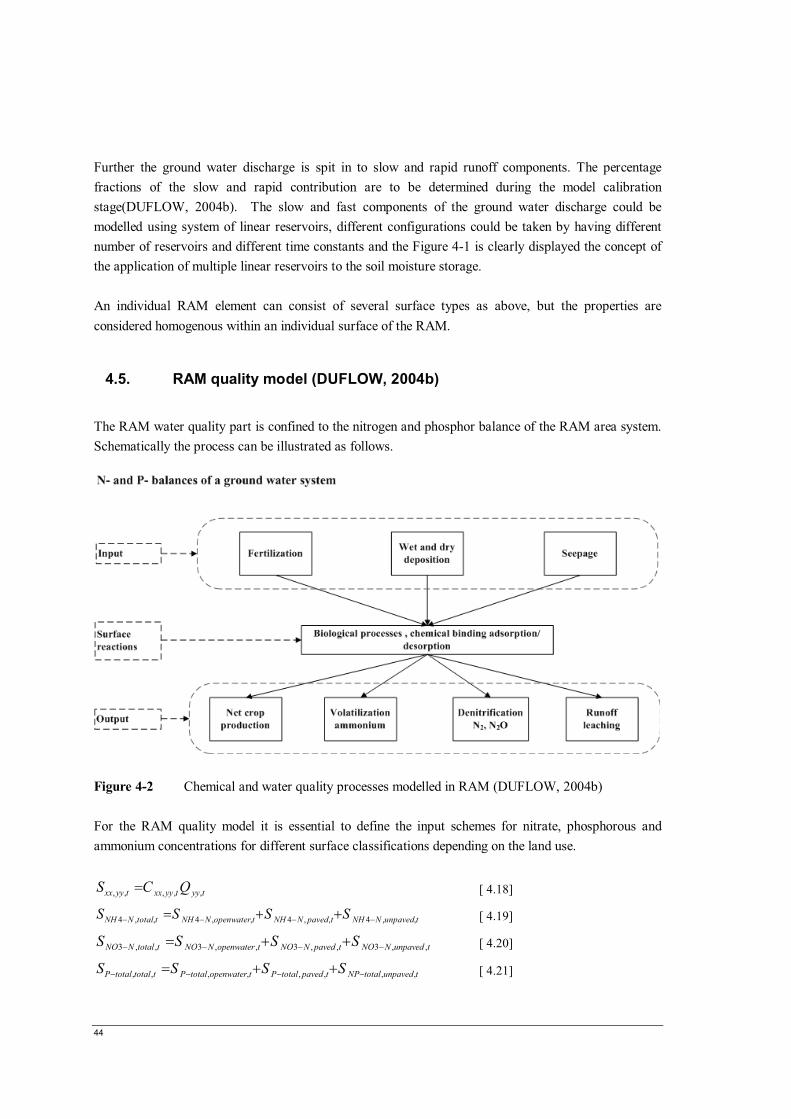
44
Further the ground water discharge is spit in to slow and rapid runoff components. The percentage fractions of the slow and rapid contribution are to be determined during the model calibration stage(DUFLOW, 2004b). The slow and fast components of the ground water discharge could be modelled using system of linear reservoirs, different configurations could be taken by having different number of reservoirs and different time constants and the Figure 4-1 is clearly displayed the concept of the application of multiple linear reservoirs to the soil moisture storage. An individual RAM element can consist of several surface types as above, but the properties are considered homogenous within an individual surface of the RAM.
4.5. RAM quality model (DUFLOW, 2004b)
The RAM water quality part is confined to the nitrogen and phosphor balance of the RAM area system. Schematically the process can be illustrated as follows.
Figure 4-2 Chemical and water quality processes modelled in RAM (DUFLOW, 2004b) For the RAM quality model it is essential to define the input schemes for nitrate, phosphorous and ammonium concentrations for different surface classifications depending on the land use.
tyytyyxxtyyxx QCS ,,,,, = [ 4.18]
tunpavedNNHtpavedNNHtopenwaterNNHttotalNNH SSSS ,,4,,4,,4,,4 −−−− ++= [ 4.19]
tunpavedNNOtpavedNNOtopenwaterNNOttotalNNO SSSS ,,3,,3,,3,,3 −−−− ++= [ 4.20]
tunpavedtotalNPtpavedtotalPtopenwatertotalPttotaltotalP SSSS ,,,,,,,, −−−− ++= [ 4.21]
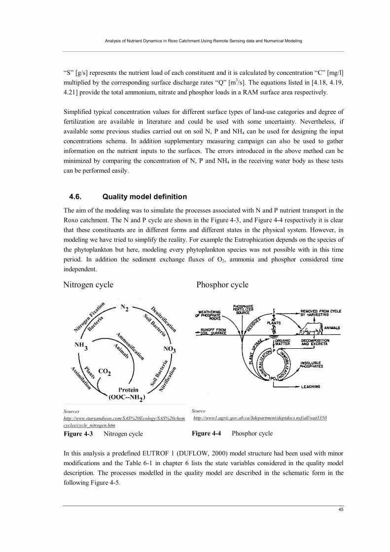
Analysis of Nutrient Dynamics in Roxo Catchment Using Remote Sensing data and Numerical Modeling
45
“S” [g/s] represents the nutrient load of each constituent and it is calculated by concentration “C” [mg/l] multiplied by the corresponding surface discharge rates “Q” [m3/s]. The equations listed in [4.18, 4.19, 4.21] provide the total ammonium, nitrate and phosphor loads in a RAM surface area respectively. Simplified typical concentration values for different surface types of land-use categories and degree of fertilization are available in literature and could be used with some uncertainty. Nevertheless, if available some previous studies carried out on soil N, P and NH4 can be used for designing the input concentrations schema. In addition supplementary measuring campaign can also be used to gather information on the nutrient inputs to the surfaces. The errors introduced in the above method can be minimized by comparing the concentration of N, P and NH4 in the receiving water body as these tests can be performed easily.
4.6. Quality model definition
The aim of the modeling was to simulate the processes associated with N and P nutrient transport in the Roxo catchment. The N and P cycle are shown in the Figure 4-3, and Figure 4-4 respectively it is clear that these constituents are in different forms and different states in the physical system. However, in modeling we have tried to simplify the reality. For example the Eutrophication depends on the species of the phytoplankton but here, modeling every phytoplankton species was not possible with in this time period. In addition the sediment exchange fluxes of O2, ammonia and phosphor considered time independent.
Sources http://www.starsandseas.com/SAS%20Ecology/SAS%20chemcycles/cycle_nitrogen.htm
Figure 4-3 Nitrogen cycle
Source http://www1.agric.gov.ab.ca/$department/deptdocs.nsf/all/wat3350
Figure 4-4 Phosphor cycle In this analysis a predefined EUTROF 1 (DUFLOW, 2000) model structure had been used with minor modifications and the Table 6-1 in chapter 6 lists the state variables considered in the quality model description. The processes modelled in the quality model are described in the schematic form in the following Figure 4-5.
Phosphor cycle Nitrogen cycle

46
Figure 4-5 Structure of the water quality model description The modified process description file is attached in the Appendix 15. Prior to the compilation and running the quality model it is essential that the flow model is stable and has been well calibrated.
4.7. Previous modeling studies with Duflow
In the literature review it was found that some studies carried out using Duflow as a basic modeling tool. Duarte et al (1999) carried out a study to compare the numerical techniques in solving dispersion problems in the river Mondego and the numerical modeling was tested with tracer injection to the river. With his results he showed that Duflow aided with hydrodynamic and water quality modeling tools provide results that show best agreement with experimental data. A flow modeling with Duflow was carried out by Windemuller et al(1997) in the Lake Okeechobee in the South Florida ecosystem because of the its importance of the lake due to the water resources for water supply and that was subjected to water quality deterioration with particulate prosperous discharged from the agriculture areas. His objective was to build and calibrate a flow model in the primary canal network as an initial stage of developing a water quality (nutrient and sediment) model. Duflow DMS had effectively being used by Ochir (2008) to model surface water quality assessment and modeling Tuul river (Mongolia) and he modelled the waste water treatment plant impacts. Efforts were made by Ochir (2008) to assess the impact on river water quality using ammonium, nitrate, nitrite, DO, COD and BOD as quality indicators using Duflow flow and quality modeling tools. Makkinga (1998) had also used DUFLOW for modeling dissolved oxygen in the river Regge was able to attain a reasonable simulation and concluded that DUFLOW is valuable tool for scenario analysis and also suitable tool to study hydrology and nutrient dynamics (Makkinga, 1998).

Analysis of Nutrient Dynamics in Roxo Catchment Using Remote Sensing data and Numerical Modeling
47
Mwannuzi et al (2003) used DUFLOW model to study the buffering effect of the wetland in lake Victoria and to assess the capacity of the wetland to absorb nutrients and other pollutants. The focus of his study was on nitrogen and phosphorus but DO, BOD, DOM, SS, EC were also included in the wetland model. He further stated that the quantity and quality are shown good agreement with the measured values and concludes that Duflow is good tool for study water quality and buffering capacity.
4.8. Model simplifications and limitations (DUFLOW)
The precipitation runoff module in DMS is developed so that processes are described at sub-catchment level and the area average value of sub catchment has to be entered as input parameters, however in reality the surface properties and parameter values vary from location to location. The capillary rise from the ground water to the unsaturated zone are not been considered. Another model simplification is that Infiltration immediately results in percolation to the deep ground water. The parameters specified in the precipitation runoff module does not have direct physical relevance and strongly empirical in nature. All equations are for one dimensional setup and model can not take in to consideration the variation on the flow in other dimensions. It models flow velocity averaged over the flow section (depth and width) though there are obvious variations. Modeling can not be performed if there is a significant difference of inflow velocity over the vertical profile (stratified wasters).

48

Analysis of Nutrient Dynamics in Roxo Catchment Using Remote Sensing data and Numerical Modeling
49
5. Integration of satellite remote sensing data
One of the objectives of this research was to investigate the possibilities of integrating remote sensing derived precipitation data in to numerical model as a driving meteorological force. In order to perform this task of integration of the remote sensing data in to the model following activities had been carried out in sequential order, downloading, pre-processing, extraction and comparison for the reliability of the remote sensing derived data sets and creating input data schemes for the model.
5.1. MSG_Multi-sensor Precipitation Estimate (MPE)
The Multi-sensor Precipitation Estimate (MPE) is a product distributed by EUMETSAT and is providing instantaneous rain rates by utilising METEOSAT data in combination with SSM/I on board US Defence Meteorological Satellite Program (DMSP). The data is provided at an intensity of mm/15min for each METEOSAT image in its original pixel resolution. Currently METEOSAT 7, 8 and 9 are being used for producing the real-time rainfall products. Rainfall data is produced by a technique called blending utilising two remote sensing data products (EUMETSAT, 2009; Heinemann et al., 2002). The concept of blending is that to utilise the high temporal and spatial resolution of geostationary Meteosat-IR sensor with high accuracy in rain rate retrieved from the microwave sensor on the polar orbiting US DMSP satellites. There are three DMSP satellite carrying SSM/I sensors (F13, F14 & F15) with approximately 6 hour repeat cycle (NGDC, 2009) . The derivation of rain rates from microwave sensors are already established (Heinemann et al., 2002) and brightness temperature calculated from the Meteosat IR channel is correlated with rainfall rates of the microwave sensor to produce MPE rain rates. This method is based on the concept that colder clouds are more likely to produce higher rain rates. Heinemann et al (2002) further explains that MPE algorithms are more appropriate in estimating convective type of rains.
5.2. MPE precipitation data
The data comes as General Regularly-distributed Information in Binary (GRIB) files and each consists of two quality indicators stated according to the Heinemann et al (2002) the standard deviation and correlation coefficient. The standard deviation and correlation coefficient is calculated considering the MSG IR sensor data and SSM/I data comparison. Heinemann et al (2002) further states that when the correlation is less than 0.4 MPE rainfall products are not suitable for the use. According to EUMETSAT these information on correlation and standard deviation are appended to the GRIB files and the information could be extracted from the standard GRIB decoder. The algorithm that is used for rainfall estimation is explained comprehensively in Heinemann et.al.(2002). In simple terms the algorithm is based on the theory that the coldest cloud temperature is

50
related to highest rainfall intensity and there is a threshold temperature value when above that no rain can occur. The used algorithm has to change geographical position and with time as it depends on the current weather situation. Due to the low temporal coverage of the microwave imager, the algorithm is not modified/revised each and every image but do it for the aggregated MSG IR images. So there are possible shortcomings in the calibration of cloud top temperature and even calibration is not performed for the entire area but just on a portion of the image.
5.3. Data formats and pre-processing
As stated in the previous paragraph MPE data comes as GRIB file format and there are 96 GRIB files on a particular day at 15 minutes time intervals. These GRIB files format had to be converted all into ILWIS through DOS based batch processing, Ultimately 96 images are aggregated to produce the daily precipitation image. The MPE data had been processed is starting from January 2007 to May 2008. The data is originally in MSG geo-reference and the projection parameters are as follows. Projection parameters Geostationary satellite Ellipsoid User defined Ellipsoid Parameters a = 6378140, 1/f =298.252981 False Easting = 0.0 False Northing = 0.0 Central Meridian = 0 0 Scale Factor = 0 1 Height Persp Center = 0 35785831 It was observed some data gaps and missing GRIB files during the study period (Jan 2007 to May 2008), and relevant information is listed in the Appendix 9. For data compilation and subsequent analysis the missing information was checked against the occurrence or rainfall measured on the ground. For these days that there was missing information no rainfall was recorded.
5.4. Data extraction
MPE data was compiled in to daily aggregated rainfall map since January 2007, there were 478 days of records (ILWIS map files) in a layer stack. The MPE rainfall image covers approximately half of the globe and to handle it conveniently, sub-maps were created so that it covers the study area. Then 18 random data extraction points had been selected from the catchment considering the size and the location of the catchment. There were one or more pointes selected from each sub catchment for subsequent rainfall data extraction. The Figure 5-1 shows the locations of the 18 points within the catchment. An ILWIS script function had been used to extract the data from rainfall image stack that consists of 478 layers. This data set was compared with the nearby weather station data for consistency checks before implementing it in the model.

Analysis of Nutrient Dynamics in Roxo Catchment Using Remote Sensing data and Numerical Modeling
51
Figure 5-1 Roxo catchment with 18 pts overlaid on top of MPE image: date 10/02/2007 (MSG geo-reference)
Comparison of MPE data with gauge station data
y = 0.831x + 54.909R2 = 0.9386
y = 0.7675x + 52.691R2 = 0.9558
0
100
200
300
400
500
600
700
0 100 200 300 400 500 600 700Cumulative of Average (18 pts MSG_MPE) precipitation (mm)
Cum
. Rai
n C
OTR
Sta
tion
Dat
a (m
m)
ppp
Beja
Aljustrel
Linear (Aljustrel)
Linear (Beja)
Figure 5-2 Comparison of MPE data and ground based data The 18 data extraction points are spatially distributed as shown in the Figure 5-1 and there were approximately 40 MSG-MPE grids/pixels falling with in the catchment. Based on the area coverage of the sub-catchment one or more point have placed in the sub catchment (e.g catchment 12 having 3
Beja
Aljustrel
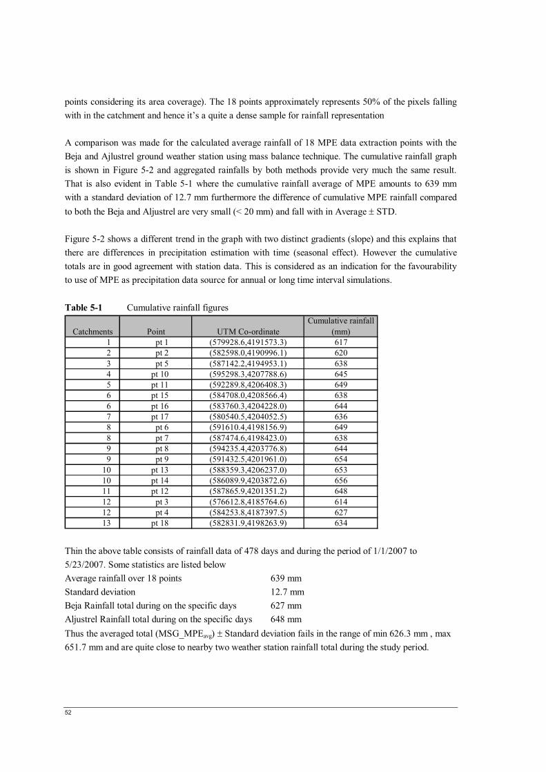
52
points considering its area coverage). The 18 points approximately represents 50% of the pixels falling with in the catchment and hence it’s a quite a dense sample for rainfall representation A comparison was made for the calculated average rainfall of 18 MPE data extraction points with the Beja and Ajlustrel ground weather station using mass balance technique. The cumulative rainfall graph is shown in Figure 5-2 and aggregated rainfalls by both methods provide very much the same result. That is also evident in Table 5-1 where the cumulative rainfall average of MPE amounts to 639 mm with a standard deviation of 12.7 mm furthermore the difference of cumulative MPE rainfall compared to both the Beja and Aljustrel are very small (< 20 mm) and fall with in Average ± STD. Figure 5-2 shows a different trend in the graph with two distinct gradients (slope) and this explains that there are differences in precipitation estimation with time (seasonal effect). However the cumulative totals are in good agreement with station data. This is considered as an indication for the favourability to use of MPE as precipitation data source for annual or long time interval simulations. Table 5-1 Cumulative rainfall figures
Catchments Point UTM Co-ordinateCumulative rainfall
(mm)1 pt 1 (579928.6,4191573.3) 6172 pt 2 (582598.0,4190996.1) 6203 pt 5 (587142.2,4194953.1) 6384 pt 10 (595298.3,4207788.6) 6455 pt 11 (592289.8,4206408.3) 6496 pt 15 (584708.0,4208566.4) 6386 pt 16 (583760.3,4204228.0) 6447 pt 17 (580540.5,4204052.5) 6368 pt 6 (591610.4,4198156.9) 6498 pt 7 (587474.6,4198423.0) 6389 pt 8 (594235.4,4203776.8) 6449 pt 9 (591432.5,4201961.0) 654
10 pt 13 (588359.3,4206237.0) 65310 pt 14 (586089.9,4203872.6) 65611 pt 12 (587865.9,4201351.2) 64812 pt 3 (576612.8,4185764.6) 61412 pt 4 (584253.8,4187397.5) 62713 pt 18 (582831.9,4198263.9) 634
Thin the above table consists of rainfall data of 478 days and during the period of 1/1/2007 to 5/23/2007. Some statistics are listed below Average rainfall over 18 points 639 mm Standard deviation 12.7 mm Beja Rainfall total during on the specific days 627 mm Aljustrel Rainfall total during on the specific days 648 mm Thus the averaged total (MSG_MPEavg) ± Standard deviation fails in the range of min 626.3 mm , max 651.7 mm and are quite close to nearby two weather station rainfall total during the study period.

Analysis of Nutrient Dynamics in Roxo Catchment Using Remote Sensing data and Numerical Modeling
53
5.5. Spatial variability of the rainfall with in the catchment
The Figure 5-3 depicts scatter plot of daily average rainfall (18 points) verses rainfall of 5 random points (pt 1, 4, 13, 15 and 18). According to the best fit line in the graph, the slope is almost equal to 1 while coefficient of determination [R2] equals to 0.9903. This explains that individual point rainfalls are very similar to the average of 18 points. Thus we can distinguish the spatial variability of the MPE rainfall with in the catchment is minimum.
Scatter plot for MPE points rainfall distribution
y = 1.0018x + 0.0065R2 = 0.9903
0
2
4
6
8
10
12
14
16
18
20
0 2 4 6 8 10 12 14 16 18 20Average rainfall (mm)
Poin
t rai
nfal
l dat
a (m
m)
jjj
pt1pt4pt13pt15pt18Linear (pt13)
Figure 5-3 Consistency check for random 5 points

54
5.6. Comparison of MPE rainfall with gauge data
The MPE performs best in strong convective type of rain, it can also detect frontal precipitation but the exact position could be misled by about 100 kms according to Heinemann et al (2003), most rainfalls in the Portugal have the strong influence of ocean and that could be one reason for the deviation. The SSM/I data used to calibrate MSG-IR rain-rates are only available at satellite overpass times possibly 3-4 times in a day. If rain does not occur during that time calibration may have problem in representing the rain rates. In addition Heinemann et al (2003) sited (Berge,2003) states that precipitation in general is underestimated by the MPE products. Thus, there are possibilities in underestimating rain rates derived through the MSG IR channel images.
5.7. Conclusion
Referring Figure 5-3 it can be said that variability with in the catchment is minimal and 18 data points are sufficient to represent the rain estimation as the spatial variability within the catchment is negligible. According to the analysis there is an inconsistency in daily rainfalls values between the MPE data and nearby ground station data. MSG MPE is a better option in a situation where there is scarcity of weather data.

Analysis of Nutrient Dynamics in Roxo Catchment Using Remote Sensing data and Numerical Modeling
55
6. Model Development and Implementation
6.1. Modeling objectives and the scope
Hydrologic and water quality models are extensively used in current context and their applications are on basically guiding water resources policy, water resources management and water resources regulations (Harmel and Smith, 2007). In this particular modeling study, it is intended to use the model for basic guidance for water quality management such are pollution control of ground and surface waters and predict the possible contaminant loads. Further this could be used to manage the drinking water quality issues. It is observed that EMAS water treatment plant at Beja uses expensive activated carbon filter media due to the risk of contamination of water with algal toxins (blue green algae). Thus the regulation and water quality management practice aided with numerical models could reduce expensive water treatment costs. The modeling study is limited to Roxo catchment having approximately 350 km2. Modeling is carried out with Duflow Modeling Studio(DMS), and emphasis is laid on the nutrients nitrates, ammonium and phosphates. Considering the availability of data, a simulation period was selected spanning from September 2001 to December 2007 and a daily time interval (temporal resolution) was selected for the analysis.
6.2. Schematization of the study area
The physical schematization is a key process in modeling. It depends on the data availability and the expected degree of accuracy of the Modeling. In this sense, Duflow allows the user to define the level of detail of the physical modeling system. To formulate the Duflow model the study area was schematized into following elements:
• Nodes, schematization points, calculation points • Stream Lines • Flow section definitions (cross section) • RAM runoff areas components • Structures (weir, discharge point WWTP )
Initially the Roxo catchment delineated using the Aster DEM was further sub-divided in to 13 sub-catchments. The number of sub catchments was decided based on the stream discharge points to the Roxo reservoir. Since Pisoes sub-catchment has more information and contains a small stream (Chamine) that is considered to be the only perennial stream of the catchment, it was divided in 4 sub catchments. The Appendix 2_fig.(d) shows the delineated sub catchments.
56
Nodes were introduces at the key points like junctions, discharge points of individual sub catchments, outlets of the streams and by both sides of structures. The streamlines were designed considering the longest flow path determined by the hydro-DEM process. The schematization points (bending) introduced so that the stream path follows the actual drainage profile on background streamline map. As a model simplification all streams sections were considered to be uniform in size and shape and it not far from reality as most channel section are found to be of a similar size in most field observations. The stream sections were considered to be trapezoidal. Each sub catchment was assigned with rainfall runoff area (RAM) component and individual RAM component was assigned following information.
• Surface classification • Rainfall and potential Evapotranspiration (ET) • Soil Parameters and surface properties • Nutrient Schemes
Natural basins show greater variability and complexity with respect to soils, land cover and topographic characteristics (Lenhart et al., 2002). In Duflow the sub basins are represented by RAM elements and each have to be provided with area average parameter values for each surface. Since each sub catchment level calibration was not possible due to the un-gauged nature of the catchment runoff, general values (area average for entire catchment) have been used so that degrees of freedom in model calibration would reduce to manageable proportion. The information used in the model for different surface types are listed in the Appendix 18. The only structure in the catchment is Roxo dam and it was modelled with a weir structure. The rain and evaporation data was available at daily time intervals and hence daily calculation steps for flow and quality were selected in the model simulations. The simulated runoff output was taken at decadal (10 day aggregated) time intervals for the model calibration and validation as to minimize the errors in the water balance calculations due to low precision of the water level measurements.
6.3. Basic data inputs and data formats
Data input can be done in different techniques in Duflow, the evaporation, precipitation, had a very long time series data and it was converted in to ASCII file format. Those ASCII files can easily be imported and define the input data schemes. In addition there is a possibility in defining data non equidistant, Fourier or constant time series settings. Water quality parameters change seasonally and hence non-equidistant time intervals were also used. The general boundary condition can be provided any of the above methods. In this model flow and head boundary conditions were given as constant values with time. The input parameters were defined in the respective menus and those are constant with time and Duflow will now allow temporal variation in parameter settings. Initial conditions are also time invariant and values were set at the beginning of the simulation.
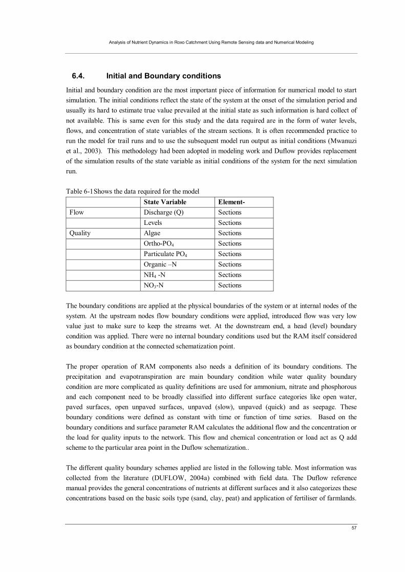
Analysis of Nutrient Dynamics in Roxo Catchment Using Remote Sensing data and Numerical Modeling
57
6.4. Initial and Boundary conditions
Initial and boundary condition are the most important piece of information for numerical model to start simulation. The initial conditions reflect the state of the system at the onset of the simulation period and usually its hard to estimate true value prevailed at the initial state as such information is hard collect of not available. This is same even for this study and the data required are in the form of water levels, flows, and concentration of state variables of the stream sections. It is often recommended practice to run the model for trail runs and to use the subsequent model run output as initial conditions (Mwanuzi et al., 2003). This methodology had been adopted in modeling work and Duflow provides replacement of the simulation results of the state variable as initial conditions of the system for the next simulation run. Table 6-1 Shows the data required for the model State Variable Element- Flow Discharge (Q) Sections Levels Sections Quality Algae Sections Ortho-PO4 Sections Particulate PO4 Sections Organic –N Sections NH4 -N Sections NO3-N Sections
The boundary conditions are applied at the physical boundaries of the system or at internal nodes of the system. At the upstream nodes flow boundary conditions were applied, introduced flow was very low value just to make sure to keep the streams wet. At the downstream end, a head (level) boundary condition was applied. There were no internal boundary conditions used but the RAM itself considered as boundary condition at the connected schematization point. The proper operation of RAM components also needs a definition of its boundary conditions. The precipitation and evapotranspiration are main boundary condition while water quality boundary condition are more complicated as quality definitions are used for ammonium, nitrate and phosphorous and each component need to be broadly classified into different surface categories like open water, paved surfaces, open unpaved surfaces, unpaved (slow), unpaved (quick) and as seepage. These boundary conditions were defined as constant with time or function of time series. Based on the boundary conditions and surface parameter RAM calculates the additional flow and the concentration or the load for quality inputs to the network. This flow and chemical concentration or load act as Q add scheme to the particular area point in the Duflow schematization.. The different quality boundary schemes applied are listed in the following table. Most information was collected from the literature (DUFLOW, 2004a) combined with field data. The Duflow reference manual provides the general concentrations of nutrients at different surfaces and it also categorizes these concentrations based on the basic soils type (sand, clay, peat) and application of fertiliser of farmlands.
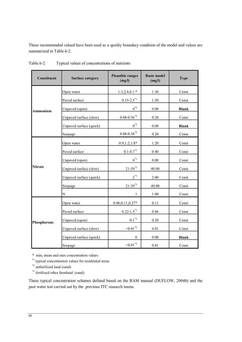
58
These recommended valued have been used as a quality boundary condition of the model and values are summarized in Table 6-2. Table 6-2 Typical values of concentrations of nutrients
Constituent Surface category Plausible ranges (mg/l)
Basic model (mg/l) Type
Open water 1.3,2.4,6.1 * 1.30 Const
Paved surface 0.15-2.5*1 1.50 Const
Unpaved (open) 0*2 0.00 Blank
Unpaved surface (slow) 0.08-0.36*2 0.20 Const
Unpaved surface (quick) 0*2 0.00 Blank
Seepage 0.08-0.36*2 0.20 Const
Open water 0.9,1.2,1.8* 1.20 Const
Paved surface 0.1-0.7*1 0.40 Const
Unpaved (open) 0*1 0.00 Const
Unpaved surface (slow) 21-39*3 40.00 Const
Unpaved surface (quick) 2*3 2.00 Const
Seepage 21-39*3 40.00 Const
N 1 1.00 Const
Open water 0.06,0.11,0.27* 0.11 Const
Paved surface 0.22-1.5*1 0.86 Const
Unpaved (open) 0-1*2 0.20 Const
Unpaved surface (slow) <0.01*2 0.01 Const
Unpaved surface (quick) 0 0.00 Blank
Seepage <0.01*2 0.01 Const
* min, mean and max concentration values*1 typical concentration values for residential areas*2 unfertilized land (sand)*3 fertilized other farmland (sand)
Ammonium
Nitrate
Phosphorous
These typical concentration schemes defined based on the RAM manual (DUFLOW, 2004b) and the past water test carried out by the previous ITC research teams.
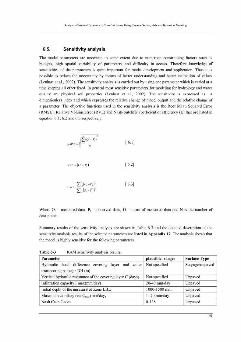
Analysis of Nutrient Dynamics in Roxo Catchment Using Remote Sensing data and Numerical Modeling
59
6.5. Sensitivity analysis
The model parameters are uncertain to some extent due to numerous constraining factors such as budgets, high spatial variability of parameters and difficulty in access. Therefore knowledge of sensitivities of the parameters is quite important for model development and application. Thus it is possible to reduce the uncertainty by means of better understanding and better estimation of values (Lenhart et al., 2002). The sensitivity analysis is carried out by using one parameter which is varied at a time keeping all other fixed. In general most sensitive parameters for modeling for hydrology and water quality are physical soil properties (Lenhart et al., 2002). The sensitivity is expressed as a dimensionless index and which expresses the relative change of model output and the relative change of a parameter. The objective functions used in the sensitivity analysis is the Root Mean Squared Error (RMSE), Relative Volume error (RVE) and Nash-Sutcliffe coefficient of efficiency (E) that are listed in equation 6.1, 6.2 and 6.3 respectively.
( )
N
PORMSE
N
iii
2
1∑
=
−= [ 6.1]
( )ii PORVE −= [ 6.2]
( )
( )∑∑
=
=
−
−−=
N
i i
N
i ii
OO
POE
1
21
2
1 [ 6.3]
Where Oi = measured data, Pi = observed data,⎯O = mean of measured data and N is the number of data points. Summary results of the sensitivity analysis are shown in Table 6-3 and the detailed description of the sensitivity analysis results of the selected parameters are listed in Appendix 17. The analysis shows that the model is highly sensitive for the following parameters. Table 6-3 RAM sensitivity analysis results Parameter plausible ranges Surface Type Hydraulic head difference covering layer and water transporting package DH (m)
Not specified Seepage/unpaved
Vertical hydraulic resistance of the covering layer C (days) Not specified Unpaved Infiltration capacity I max(mm/day) 20-40 mm/day Unpaved Initial depth of the unsaturated Zone LBv0 1000-1500 mm Unpaved Maximum capillary rise Cmax (mm/day) 1- 20 mm/day Unpaved Nash Cash Cades 0-128 Unpaved
60
6.6. Model calibration
The calibration is the process by which a output of the model is matched with the observed field data. Generally in hydraulic Modeling flow observations are matched by changing the input parameters. As illustrated before only measurement available in this catchment is the reservoir water levels and abstractions, and the reservoir inflow time series derived from these data. The flow model calibration was performed by adjusting the different parameters of the model and plausible ranges of some the parameters were found from the literature. In addition there are guide lines in the Duflow user manual for some parameter values (reservoir constants reservoir [k], initial storage [Bmax], etc.). The calibration was done for the period starting from the Sep 2001 to Dec 2004 period and the discharge results were aggregated at ten days intervals (decadal). The calibration at individual sub-catchment parameter setting was not feasible as the sub catchments were not gauged at their individual outlet points. The goodness of fit was assessed by the considering the Root Mean Squared Error as listed in the equation [6.1] and visual examination of the behaviour of the simulated hydrograph. The Table 6-3 below shows the calibrated flow model and the Appendix 18 list out the adjusted parameters. The flow model calibration produces relatively acceptable runoff simulation pattern with calculated inflows, however some peak are not perfectly coincide with the calculate inflows. The goodness of fit values shows that it is of an acceptable order. However model could have been better calibrated still if it had actual gauge measurements. The inflow values calculated based on the reservoir water balance show that there were some negative values appearing and this can be explained by the accuracy in the level measurements, under estimated discharge from the reservoir or even it could be due to actual evaporation from the water surface, which can be higher than the calculated. In addition some of the simplifications made during schematization and parameterization of the model could also affect the accuracy of the simulated discharge. The general surface properties of sub-catchments were assumed to be uniform during the model building, but in reality due to the diverse nature of the soil prevailed in the catchment the resultant (area average) parameter values could be deferent from what had been used in the model at individual catchments. Thus each catchment could have its own optimum parameter setting, but due the limitation in calibration data and time constraint. This prompt us to simplify the model at this stage.
6.7. Model validation
The validation is the process by which a second set of independent stress conditions are applied to the model to test and assure the reliability, accuracy and predictive capability of the model. Initially the flow model parameters were calibrated for stress conditions of just 3 years and the next 3 years are used for the validation. Since there was a very long drought period there was a long time period where zero or no flow conditions and there were major runoff can be observed during Oct-Dec 2006 and it has been simulated perfectly well. The results show in Figure 6-2 that the flow model is simulating the inflow condition reasonably well.

Analysis of Nutrient Dynamics in Roxo Catchment Using Remote Sensing data and Numerical Modeling
61
Model Calibration- Decadal stream flow (m3/sec)
0
1
2
3
4
5
6
7
8
9
10Se
p-01
Oct
-01
Oct
-01
Nov
-01
Dec
-01
Jan-
02
Feb-
02
Mar
-02
Apr
-02
May
-02
Jun-
02
Jul-0
2
Aug
-02
Sep-
02
Oct
-02
Nov
-02
Dec
-02
Jan-
03
Feb-
03
Mar
-03
Apr
-03
May
-03
Jun-
03
Jul-0
3
Aug
-03
Sep-
03
Oct
-03
Nov
-03
Dec
-03
Jan-
04
Feb-
04
Mar
-04
Apr
-04
May
-04
Jun-
04
Jul-0
4
Aug
-04
Sep-
04
Oct
-04
Nov
-04
Dec
-04
Time
Dec
adal
inflo
w (m
3 /sec
) d
dddd
Decadal inflow (m3/sec)Model output (m3/sec)
Figure 6-1 Model calibration: simulated discharge vs. observed runoff
Model Validation - Decadal stream flow (m3/sec)
0
2
4
6
8
10
12
14
16
18
20
22
24
26
Sep-
04
Oct
-04
Nov
-04
Dec
-04
Jan-
05
Feb-
05
Mar
-05
Apr
-05
May
-05
Jun-
05
Jul-0
5
Aug
-05
Sep-
05
Oct
-05
Nov
-05
Dec
-05
Jan-
06
Feb-
06
Mar
-06
Apr
-06
May
-06
Jun-
06
Jul-0
6
Aug
-06
Sep-
06
Oct
-06
Nov
-06
Dec
-06
Jan-
07
Feb-
07
Mar
-07
Apr
-07
May
-07
Jun-
07
Jul-0
7
Aug
-07
Sep-
07
Oct
-07
Nov
-07
Dec
-07
Time
Dec
adal
inflo
w (m
3 /sec
)
Decadal inflow (m3/sec)
Model output (m3/sec)
Figure 6-2 Model validation: simulated discharge vs. observed runoff

62
In addition, the peak flows correspond to each other and there is a small time shift which can be due to (a) possible errors of having reservoir water levels records (b) the number of RAM element used in the modeling, which could have been improved by splitting the sub catchments further into few more RAM elements and introducing surface properties that corresponds to each sub catchment. With the validation results, the model is considered sufficiently adjusted for the subsequent water quality modeling process.
6.8. Results-water quality (nutrient) modeling
The results of the water quality simulation are as shown in the Figure 6-5 below. It is observed that the there are concentration fluctuations in the ammonium and nitrate at the reservoir. It is clear that nitrate concentration is usually high in November-March. This can be explained by the higher nitrate flow to the river after every rain event. The nitrate concentration is fluctuating around 2.5 mg/l at the peak while it can be low as 0.3 mg/l during months with lowest concentrations. According to the Figure 6-6b the ammonium concentrations are very low in the reservoir and this agrees with the field concentration measurements made during the early Oct 2008.
Figure 6-3 Duflow model structure showing all key elements
Figure 6-4 Nitrification along the main river (Chamine) section
The above Figure 6-4 shows the Nitrification process (Nitrification: the oxidation of ammonia to nitrate, via nitrite) occurring along the main river stretch. NH3 + CO2 + 1.5 O2 + Nitrosomonas → NO2
- + H2O + H+ NO2
- + CO2 + 0.5 O2 + Nitrobacter → NO3-
With this result, it can be stated that the quality model reasonably simulate the process of nitrification happening along the river and the concentration are also with in the observations.

Analysis of Nutrient Dynamics in Roxo Catchment Using Remote Sensing data and Numerical Modeling
63
The simulation results for the phosphorous does not show reasonable concentration observed in the Roxo reservoir. Generally the values are less than 0.2 mg/l while model simulates relatively higher phosphate concentrations in the reservoir (see. Appendix 19) and this could be mainly due to the fact that model may not adequately describe the phosphate interaction with in the system, especially the interactions with the bed sediments,. Hence phosphor description needs further refinement and in the quality model description.
6.9. Scenario analysis
A Duflow scenario was built to make a comparison of the runoff generation in the Roxo catchment based on the two rainfall methods. In this analysis the daily precipitation from the ground stations and the MSG-MPE were considered for 1.5 years period. The runoff generated from MSG-MPE was compared with that of measured flow based on the reservoir water balance technique which was available from Jan 2007 till Dec 2007 (one year). All the data processing was carried out at equivalent daily time steps. The results are plotted in Figure 6-7 and it is evident that gauge station data is inline with the runoff calculated by RWBT. However MSG shows large runoff during the month of Sep 2007 amounting approx 42 m3/s and other two runoffs methods (gauge and calculated) are not showing such a peak runoff on sep 2007 moreover the year 2007 is considered as a dry year without major inflow to the reservoir. Hence the runoff shown in MPE data integrated scenario can be considered as a result generated du to an out liar. In addition MPE shows rather strange results in the year 2008 with two major flow one is rather low in magnitude (Feb 2008) and isolated runoff in March 2008. The Figure 6-8 shows the cumulative rainfall change of MPE and two COTR weather stations during the selected time period and this clearly indicates the changes occurring in the rainfall and during Sep 2007 and Apr 2008 MPE shows very high rainfall values in comparison to the two automatic weather stations. These high rainfall values are leads to generate high runoff events during those time periods in model.

64
Fi
g. (b
) Tem
pora
l var
iatio
n of
nitr
ate
conc
entra
tion
at th
e R
oxo
rese
rvoi
r sec
tion
Fig.
( (d
) Te
mpo
ral
varia
tion
in a
mm
oniu
m c
once
ntra
tion
at R
oxo
rese
rvoi
r se
ctio
n
Fi
g.( a
)Nitr
ate
conc
entra
tion
varia
tion
alon
g th
e st
ream
sect
ions
Fi
g. (c
) A
mm
oniu
m c
once
ntra
tion
chan
ge a
long
the
stre
am se
ctio
ns
Figure 6-5 Temporal variation of the nitrate, ammonium concentrations
Varia
tion o
f Nitra
te co
ncen
tratio
n
05101520253035404550 Sep-
01Fe
b-02
Aug-
02Fe
b-03
Aug-
03Fe
b-04
Aug-
04Fe
b-05
Aug-
05Fe
b-06
Aug-
06Fe
b-07
Aug-
07
Date
Nitrate concentration (mll)
SEC2
:SCH0
0022
->CL
C000
08 SE
C2:CL
C000
03->C
LC00
004
SEC2
:CLC
0001
5->CL
C000
16 SE
C2:C
LC00
029->
CLC0
0030
SEC3
:CLC
0003
1->CL
C000
32 SE
C3:CL
C000
57->C
LC00
058
SEC4
:CLC
0006
3->CL
C000
64 SE
C4:C
LC00
074->
CLC0
0075
SEC1
4:CLC
0010
4->CL
C001
05 SE
C15:C
LC00
115->
CLC0
0116
SEC1
6:CLC
0012
3->CL
C001
24 SE
C28:C
LC00
211->
CLC0
0212
Am
mom
ium C
once
ncen
tratio
n alo
ng P
isoes
rive
r
051015202530354045 Sep-
01Fe
b-02
Aug
-02
Feb-
03A
ug-0
3Fe
b-04
Aug
-04
Feb-
05A
ug-0
5Fe
b-06
Aug
-06
Feb-
07A
ug-0
7
Tim
e
Ammonium Concentration (mg/l)
SEC
2:SC
H00
022-
>CL
C000
08 S
EC2:
CLC
0001
5->C
LC00
016
SE
C2:C
LC0
0029
->CL
C000
30 S
EC2:
CLC
0000
3->C
LC0
0004
SEC
2:C
LC00
004-
>CLC
0000
5 S
EC3:
CLC
0003
1->C
LC00
032
SE
C3:C
LC0
0057
->CL
C000
58 S
EC4:
CLC
0006
3->C
LC0
0064
SEC
4:C
LC00
074-
>CLC
0007
5 S
EC15
:CL
C001
15->
CLC
0011
6 S
EC1
6:CL
C001
23->
CLC0
0124
SEC
28:C
LC00
211-
>CLC
0021
2
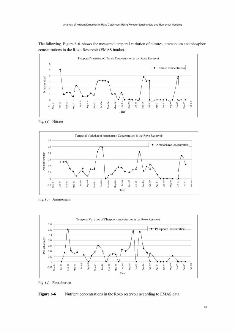
Analysis of Nutrient Dynamics in Roxo Catchment Using Remote Sensing data and Numerical Modeling
65
The following Figure 6-6 shows the measured temporal variation of nitrates, ammonium and phosphor concentrations in the Roxo Reservoir (EMAS intake).
Temporal Variation of Nitrate Concentration in the Roxo Reservoir
-1
0
1
2
3
4
5
6
Nov
-04
Jan-
05
Mar
-05
May
-05
Jul-
05
Sep-
05
Nov
-05
Jan-
06
Mar
-06
May
-06
Jul-
06
Aug
-06
Oct
-06
Dec
-06
Feb-
07
Apr
-07
Jun-
07
Aug
-07
Oct
-07
Dec
-07
Feb-
08
Time
Nitr
ates
mg/
l
Nitrate Concentration
Fig. (a) Nitrate
Temporal Variation of Ammonium Concentration in the Roxo Reservoir
-0.1
0
0.1
0.2
0.3
0.4
0.5
0.6
Nov
-04
Jan-
05
Mar
-05
May
-05
Jul-
05
Sep-
05
Nov
-05
Jan-
06
Mar
-06
May
-06
Jul-
06
Aug
-06
Oct
-06
Dec
-06
Feb-
07
Apr
-07
Jun-
07
Aug
-07
Oct
-07
Dec
-07
Feb-
08Time
Am
mon
ium
mg/
l
Ammonium Concentration
Fig. (b) Ammonium
Temporal Variation of Phosphor concentration in the Roxo Reservoir
-0.02
0
0.02
0.04
0.06
0.08
0.1
0.12
0.14
Nov
-04
Jan-
05
Mar
-05
May
-05
Jul-0
5
Sep-
05
Nov
-05
Jan-
06
Mar
-06
May
-06
Jul-0
6
Aug
-06
Oct
-06
Dec
-06
Feb-
07
Apr
-07
Jun-
07
Aug
-07
Oct
-07
Dec
-07
Feb-
08
Time
Phos
phor
mg/
l
Phosphor Concentration
Fig (c) Phosphorous Figure 6-6 Nutrient concentrations in the Roxo reservoir according to EMAS data
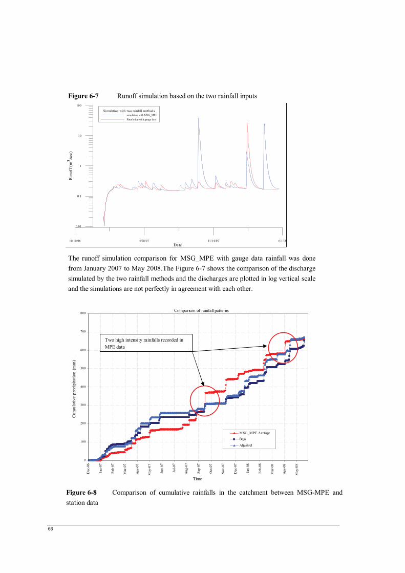
66
Figure 6-7 Runoff simulation based on the two rainfall inputs The runoff simulation comparison for MSG_MPE with gauge data rainfall was done from January 2007 to May 2008.The Figure 6-7 shows the comparison of the discharge simulated by the two rainfall methods and the discharges are plotted in log vertical scale and the simulations are not perfectly in agreement with each other.
Figure 6-8 Comparison of cumulative rainfalls in the catchment between MSG-MPE and
station data
Comparison of rainfall patterns
0
100
200
300
400
500
600
700
800
Dec
-06
Jan-
07
Feb-
07
Mar
-07
Apr
-07
May
-07
Jun-
07
Jul-0
7
Aug
-07
Sep-
07
Oct
-07
Nov
-07
Dec
-07
Jan-
08
Feb-
08
Mar
-08
Apr
-08
May
-08
Time
Cum
ulat
ive
prec
ipita
tion
(mm
) j
MSG_MPE Average
Beja
Aljustrel
Two high intensity rainfalls recorded in MPE data
10/10/06 4/28/07 11/14/07 6/1/08Date
0.01
0.1
1
10
100
Runo
ff (m
3 /sec)
Simulation with two rainfall methodssimulation with MSG_MPESimulation with gauge data

Analysis of Nutrient Dynamics in Roxo Catchment Using Remote Sensing data and Numerical Modeling
67
7. Conclusion and recommendation
7.1. Conclusion
The aim of this research was to build a numerical water quality Modeling and analysis scheme for the upper Roxo reservoir watershed. The Duflow Modeling Studio (DMS v.3.8.2) and an inverted reservoir water balance approach was used for calibration and validation of the flow model. The second aim was to investigate the possibilities of using remote sensing data (satellite precipitation) in Duflow, more specifically to force the rainfall runoff sub-model RAM. Duflow is an integration of hydrodynamics, morphology and water quality (Van Waveren et al., 1999) and a model was build for Modeling the nutrient dynamics of the upper Roxo agricultural catchment. The emphasis was on Modeling of reservoir inflows including nutrients, ammonium, nitrate and phosphorus. RAM, the rainfall runoff module was used extensively to model the water quality of land-based runoff i.e. the diffuse source pollution. Each RAM area, defining a user-defined sub-catchment was defined with different land cover inputs as well as surface and soil parameter settings as a function of availability of information. The conceptual linear reservoir based RAM model needs a considerable amount of parameters to be defined and not all those do have always physical meanings or are directly related to the physical basin properties as e.g. the reservoir time constants (DUFLOW, 2004a). The specific conclusions made in this research can be resumed as follows:
7.1.1. Estimation of runoff
The reservoir water balance calculation basically relied on registered reservoir water level fluctuations, meteorological (e.g. evaporation) and the reservoir water demand / consumption data. The reservoir inflow calculation, by basically inverting the balance equations (Eqs. 3.4 to 3.6) was done at different time steps (daily, decadal and monthly) for the past 18 years period. The reservoir water balance calculation provided the all important inflow information from the catchment to the reservoir. The calculation showed some minor negative values in the flow values, at some time periods. This could be explained by the relatively low precision of the level measurements (1 cm) or an underestimation of reservoir water releases, and uncertainties in lake evaporation and groundwater in/outflows. However, this uncertainty effect has been substantially overcome by considering decadal inflow values. Basically, the flow calibration and validation was performed using the peak runoff flows occurring during the strong rainfall events and those are only minimally affected by the precision of the level measurements.
7.1.2. Numerical flow and water quality Modeling
The predictions made by the model for the flow simulation can be considered satisfactory even with several simplifying assumptions. The model calibration and validations were done with decadal inflow (m3/sec) figures. However it was found that model predictions are somewhat peculiar at early stages of
68
the Modeling period, while the validation period (2005-2007) is well simulated, showing a Nash & Sutcliff (NS) coefficient close to 0.8 and Relative Volume Error (RVE) value within 5% range from the measured. The Duflow water quality model definitions considered processes as denitrification, nitrification, growth of algae (eutrophication) and phosphor decay. The results of the water quality simulations show a reasonable agreement and are in range with the EMAS measured data. Especially the nitrates (NO3-) show typical concentration values (0.5-5.5 mg/l) as observed in the Roxo reservoir and the temporal variation of NO3- shows relative peaks during winter months (November- March) that is quite similar to the EMAS monthly NO3 concentration data set. This agreement also prevails for the ammonium (NH4+) concentration equally showing very low values at the reservoir. Further we could clearly identify the fast nitrification process occurring on the Pisões stream after the WWTP effluent discharge point. These results are quite similar to the results obtained by Wriedt (2007) and in his analysis NO3-N concentration has seasonal dynamic and the nitrate dynamics are partly due to the drying and wetting pattern of the basin. The study shows that the surface water nitrate concentration is positively related to discharge and this can be explained by seasonality of soil leaching, increased denitrification during summer months and plant uptake of nitrogen (Dhondt et al., 2002; Wriedt et al., 2007). The study shows the highest nitrate concentration in winter coinciding the high runoff and ground water discharge and lowest in summer months coinciding the low flows and low ground water discharge.
7.1.3. Integration of rainfall remote sensing data in Duflow
The investigation of the possibility of integrating rainfall remote sensing data i.e. the MSG-MPE or Meteosat multi sensor precipitation estimate into the numerical model (Duflow) as rainfall forcing or input was one of the primary objectives of the research. The whole integration process was considered satisfactory from pre-processing up to generate the rainfall time series inputs to the model. MSG-MPE time series can be coupled to user-defined RAM areas as precipitation boundary condition. In the analysis we found that MSG-MPE data in this particular study area in Southern Portugal were not always fully in agreement with observed rainfall from ground station data. As discussed in the previous Chapter 6, the there were two strong storm events recorded in the MSG-MPE dataset, but those rainfall incidents were not recorded with the same depth by the ground weather stations. Further the calculated catchment runoff or reservoir inflows with the reservoir water balance technique were more in agreement with measured station rainfall values. Thus the MSG-MPE data are still not entirely safe for predicting precipitation for individual or daily storm events. When the model is set on a daily or sub-daily time step, one should be careful for using only satellite precipitation data for driving the model. This can be explained partly that the precipitation pattern in Portugal is usually governed by stratiform rainfall from Atlantic depressions, which is also known as frontal rain or cyclonic rain. But the MSG-MPE is best suited for predicting more convective type of rainfall, that usually has high rainfall intensities and is concentrated to particular area (Heinemann et al., 2002). Heinemann et al.(2002) indicates that the algorithms used in estimating rainfall rate initially correlates microwave SSM/I rain rates to brightness temperature of MSG TIR 10.8 um channel and that brightness temperature is near independent of the SSM/I precipitation in frontal precipitations. As such it is quite difficult to perform rainfall estimations with this algorithm in such geographic areas.
Analysis of Nutrient Dynamics in Roxo Catchment Using Remote Sensing data and Numerical Modeling
69
In contrast, as shown in Chapter 5 (Fig.5.2), the cumulative long-term or annual rainfall sums derived from MSG-MPE data, coincide very well with all the station data. This could be due to the fact that integral conserving characteristic of the matching algorithm (Heinemann et al., 2002). This permits us to use the MSG-MPE data for seasonal or annual rainfall estimations in this area. The duration of analysis is however not sufficient to draw a strong conclusion but further studies would enlighten the application of MSG-MPE in this sense. Another technique which can be proposed is to use data assimilation techniques, by which satellite and ground observations are coupled to improve the rainfall estimates and inputs for the model. This is recommended for further study.
7.2. Recommendation
The model could have been further refined in case there were few flow gauge stations at least for the major stream discharge points to the reservoir. This could yield better and more extensive RAM surface definitions, via calibration. In such case, RAM elements can be more extensively used to model more detailed semi-distributed runoffs and nutrient dynamics. A major problem encountered in using the precipitation runoff module elements in the hydraulic Modeling is that the information on the parameters and its plausible ranges are not easily found in literature. Due to the conceptual nature of the precipitation runoff module (RAM), the parameter definition process is by calibration with not always direct physical meaning (DUFLOW, 2004a). The Corinne land cover dataset Level 2 was used to parameterize the surface conditions (vegetation, crops, etc.) of the RAM areas. This dataset corresponded well with the Landsat ETM imagery and field observations. This land classification plays a major part in RAM area definitions and in addition it is used for derivation of the resultant (weighted) crop coefficients at the sub-catchments level. Thus a more comprehensive model could theoretically be developed with the use of high spatial resolution images. Further it was more useful if the RAM component of Duflow would also have the capability of importing direct GIS data (land cover, soil properties, rainfall maps etc.). Only the Duflow main engine has this capability (flow network). Our GIS source data needed to be converted to ASCII file formats prior to import into RAM and this makes model setup time consuming. The coupling of the Duflow RAM with GIS further would enhance the user friendliness and is more research time available for other process subject areas. In addition, we could not find many publications that were relevant to the use of the RAM rainfall runoff module of Duflow, where according this research, it has good potential of doing hydrologic as well as diffuse pollution Modeling. This issue make it also difficult to find the published parameters values typical for specific local conditions. Basically all starting values were based on the guidelines provided in the Duflow manual and own hydrological judgement. These initial guesses in combination with many parameters make it difficult to perform sensitivity analysis. To do an effective hydrologic or water quality Modeling, an essential requirement is information and calibration data and we could have done a much detailed analysis with still more experimental data.

70
The negative values of the reservoir balance inflow calculation could be due to different reasons such as � Low precision of the level measurements as stated above: the current water level records are
available at nearest 1 cm precision and it is low precision compared to the order of the evaporation and precipitation data. That may lead to a possible uncertainty of ±5 mm in each water level reading and can lead have ± 0.45 m3/sec uncertainty in the individual daily readings (considering an average surface area of 8 km2);
� Uncertainties in estimation of water surface evaporation: Ali (2008) in his paper explains that
precise estimation of evaporation from a water body requires extensive databases and often becomes very difficult to select the most appropriate single evaporation method. Consequently the accuracy of the method will improve the reliability of the results obtained in the water balance calculation.
� Demand and reservoir water release data: It is generally possible that water releases that were recorded in the ABROXO data could at some time points be underestimating the amounts of water released. In addition when calculating daily water balances monthly demand data have been distributed evenly over the days. That might also lead to some inaccuracies in the calculation.
Integration of remote sensing data has been carried out satisfactorily through the results are not as good as expected, especially for some individual daily time step rainfall runoff estimations. The MSG-MPE product is quite useful as it provides rainfall intensities at 15 minutes intervals (96 images per day). The processing and data extraction is somehow tedious task but can be automated. It would be better if more studies are carried out in developing an active data screening system in extracting data (at points, space windows, intensity graphs, etc) followed by subsequent data processing. The observed short term rainfall patterns were at some periods quite different from the ground observations. It is recommended to perform more MSG-MPE data application research to assess the validity of the MSG-MPE algorithm and data. Heinemann et al (2002) in his paper recommends that MSG-MPE best suited for tropical African conditions, so more investigations are needed and more applications in higher latitude areas. He further explains that validity of the blending technique and its application to semi arid climates can vary. In addition it is stated in the literature that MSG-MPE is not the best to estimate rainfall occurring in frontal weather systems. Thus it could be one reason for the discrepancies found between the MSG-MPE rainfall and ground rainfall observations. More research on algorithm adjustment or data assimilation is recommended here to improve the estimates.
Analysis of Nutrient Dynamics in Roxo Catchment Using Remote Sensing data and Numerical Modeling
71
References
Abrams, M., 2000. The Advanced Space-borne Thermal Emission and Reflection Radiometer (ASTER): data products for the high spatial resolution imager on NASA's Terra platform. International Journal of Remote Sensing, 21(5): 847 - 859.
Alam, M.G.M., Jahan, N., Thalib, L., Wei, B. and Maekawa, T., 2001. Effects of environmental factors on the seasonally change of phytoplankton populations in a closed freshwater pond. Environment International, 27(5): 363-371.
Ali, S., Ghosh, N.C. and Singh, R., 2008. Evaluating best evaporation estimate model for water surface evaporation in semi-arid region, India. Hydrological Processes, 22(8): 1093-1106.
Allen, R.G., Pereira, L.S., Raes, D. and Smith, M., 1998. Crop evapotranspiration : guidelines for computing crop water requirements. FAO irrigation and drainage paper 56. FAO, Rome (Italy), 300 pp.
Awino, F.B., 2003. Groundwater chemistry and quality assessment in Pisoes catchment, Alentejo province, southern Portugal, ITC, Enschede.
Bhandari, A., 2004. Estimation of crop water requirements for different crops and evaluation of irrigation practices in Pisoes catchment, Beja, southern Portugal : a case study, using CropWat, GIS and RS, ITC, Enschede.
Butterworth, J.A., Hewitt, E.J. and McCartney, M.P., 2000. Discharge measurement using portable dilution gauging flow meters. Journal of the Chartered Institution of Water and Environmental Management, 14(6): 436-441.
Caetano, M. and Araújo, A., 2006. Comparing land cover products CLC2000 and MOD12Q1 for Portugal. In: A. Marçal (Editor), Global Developments in Environmental Earth Observation from Space Millpress- Rotterdam, Porto, Portugal, pp. 469-477.
Caetano, M., Mata, F. and Freire, S., 2006. Accuracy assessment of the Portuguese CORINE Land Cover map. In: A. Marçal (Editor), Global Developments in Environmental Earth Observation from Space Millpress- Rotterdam, Porto, Portugal, pp. 459-467.
Cardoso, J.V.D.C., 1965. “ OS Solos De Portugal” Sua Classificação,Caracterízação E Génese, 1-A SUL DO RIO Tejo, .
CGIAR-CSI, 2009. SRTM 90m Digital Elevation Data. Consultative Group for International Agriculture Research (CGIAR), Consortium for Spatial Information, http://srtm.csi.cgiar.org/, (accessed on February 9, 2009)
Chapman, D., 1996. Water quality assessments: a guide to the use of biota, sediments and water in environmental monitoring. Spon, London etc., 626 pp.
Chapra, S.C., 1997. Surface water quality modeling. McGraw-Hill, Boston etc., 843 pp. Chen, C.H., Liu, W.L., Liaw, S.L. and Yu, C.H., 2005. Development of a dynamic strategy planning
theory and system for sustainable river basin land use management. Science of the Total Environment, 346(1-3): 17-37.
Chisha, M., 2005. Assessment of nutrient pollution contribution of the Outeiro catchment to the Roxo lake in Portugal using the GWLF model, ITC, Enschede, 77 pp.
Clemmens, A.J., Holly, F.M. and Schuurmans, W., 1993. Description and Evaluation of Program - Duflow. Journal of Irrigation and Drainage Engineering-ASCE, 119(4): 724-734.
CNPGB, 2009. Portuguese National Committee of Large Dams , Roxo Dam, http://cnpgb.inag.pt/gr_barragens/gbingles/FichasIng/RoxofichaIng.htm, (accessed on February 13, 2009).
Conference on Mediterranean Soils, 1966. Study tour through Southern Portugal : September 24 - 28 1966. International Soil Science Society, 122 pp.
72
Conteh, F., 2003. Water quality assessment, analysis and interpretation in Pisoes and part of Roxo sub - catchments, Beja, Alentejo region, Portugal, ITC, Enschede.
Dhondt, K., Boeckx, P., van Cleemput, O., Hofman, G. and de Troch, F., 2002. Seasonal groundwater nitrate dynamics in a riparian buffer zone. E D P Sciences, pp. 747-753.
Dingman, S.L., 2002. Physical hydrology. Prentice Hall, Upper Saddle River, 646 pp. Dodds, W.K. and Oakes, R.M., 2006. Controls on nutrients across a prairie stream watershed: Land use
and riparian cover effects. Environmental Management, 37(5): 634-646. Dost, R.J.J. (Editor), 2006. Water Quality Sampling and Testing Field Guide. ITC, Enschede, 136 pp. Duarte, A.A.L.S., Pinho, J.L.S., Vieira, J.M.P. and Boaventura, R.A.R., 1999. Comparison of
numerical techniques solving longitudinal dispersion problems in the river Mondego. In: E.A.E. Oliveira, J. Bento and E. Pereira (Editors), International Conference on Enhancement and Promotion of Computational Methods in Engineering and Science Elsevier, Macao, pp. 1450.
DUFLOW, 2000. DUFLOW for Windows V3.3: DUFLOW modelling studio: user’s guide, reference guide DUFLOW, and reference guide RAM, EDS/STOWA, Utrecht, The Netherlands.
DUFLOW, 2004a. Duflow Modelling Studio :Duflow Manual. Stowa/MX.Systems, pp. 112. DUFLOW, 2004b. Duflow Modelling Studio: RAM manual Precipitation Runoff Module, 3.7.
Stowa/MX.Systems. EUMETSAT, 2009. Multi-Sensor Precipitation Estimate.
http://www.eumetsat.int/Home/Main/Access_to_Data/Meteosat_Meteorological_Products/Product_List/SP_1119538666663?l=en(Accessed (accessed on February 9, 2009).
FOTW, 2009. Flags of the World - Presentation of Beja, Beja Municipality, Portugal, http://flagspot.net/flags/pt-bja.html , (accessed on February 12, 2009).
Gurung, R.P., 2007. Modelling of Eutrophication in Roxo reservoir, Alentejo, Portugal : A system dynamic based approach, ITC, Enschede, 100 pp.
Harmel, R.D. and Smith, P.K., 2007. Consideration of measurement uncertainty in the evaluation of goodness-of-fit in hydrologic and water quality modeling. Journal of Hydrology, 337(3-4): 326-336.
Heinemann, T. and Kerényi, J., 2003. The Eumetsat Multi-sensor Precipitation Estimate (MPE): Concept and validation. Proceedings of the EUMETSAT users conference , Weimar, Germany, 2003.
Heinemann, T., Lattanzio, A. and Roveda, F., 2002. The Eumetsat Multi-sensor Precipitation Estimate (MPE). Proceedings of the second International Precipitation Working Group (IPWG) meeting, Madrid, Spain, September 2002.
Hirano, A., Welch, R. and Lang, H., 2003. Mapping from ASTER stereo image data: DEM validation and accuracy assessment. Elsevier Science Bv, pp. 356-370.
Hounslow, A.W., 1995. Water quality data : analysis and interpretation. CRC Lewis, Boca Raton etc., 397 pp.
Khatsuria, R.M., 2005. Hydraulics of Spillways and Energy Dissipators. Environment International, 29. Published by CRC Press, 649 pp.
Lenhart, T., Eckhardt, K., Fohrer, N. and Frede, H.G., 2002. Comparison of two different approaches of sensitivity analysis. Physics and Chemistry of the Earth, Parts A/B/C, 27(9-10): 645-654.
Leston, S., Lillebo, A.I. and Pardal, M.A., 2008. The response of primary producer assemblages to mitigation measures to reduce eutrophication in a temperate estuary. Estuarine, Coastal and Shelf Science, 77(4): 688-696.
LPDAAC, 2001. ASTER Digital Elevation Model (DEM) Product Description, http://asterweb.jpl.nasa.gov/content/03_data/01_Data_Products/DEM.PDF, (accessed on February 8, 2009).
Maathuis, B.H.P. and Wang, L., 2006. Digital elevation model based hydro - processing. Geocarto International : a multi - disciplinary journal of remote sensing, 21(1).
Makkinga, A.A., 1998. Modelling dissolved oxygen in the river Regge system using Duflow. In: European Water Management, 1(1998)1, pp. 37-42.
Mannaerts, C.M.M., 2003. Stage-area relationship curve based on bathymetric survey data: Roxo reservoir, Beja, Portugal (Through personal communication).

Analysis of Nutrient Dynamics in Roxo Catchment Using Remote Sensing data and Numerical Modeling
73
Mannaerts, C.M.M., 2006. Stage volume relationship curve: Roxo reservoir, Beja, Portugal (Through personal communication).
Mwanuzi, F., Aalderink, H. and Mdamo, L., 2003. Simulation of pollution buffering capacity of wetlands fringing the Lake Victoria. Environment International, 29(1): 95-103.
NASA-JPL, 2009. ASTER Digital Elevation Model – AST14DEM-Relative, Jet Propulsion Laboratory, California Institute of Technology, Pasadena, California. http://asterweb.jpl.nasa.gov/content/03_data/01_Data_Products/release_DEM_relative.htm#4.%20Version%20History, (accessed on February 09, 2009)
Neal, C. et al., 2008. Water quality along a river continuum subject to point and diffuse sources.
Journal of Hydrology, 350(3-4): 154-165. NGDC, 2009. DMSP Data Availability, http://www.ngdc.noaa.gov/dmsp/availability.html, (accessed
on February 9, 2009). Ochir, A., 2008. Surface water quality assessment and modelling a case study in the Tuul river,
Ulaanbaatar city, Mongolia, ITC, Enschede, 87 pp. Poor, C.J. and McDonnell, J.J., 2007. The effects of land use on stream nitrate dynamics. Journal of
Hydrology, 332(1-2): 54-68. Ricardo Rodriguez, J.E., 2003. Influence of wastewater treatment plant on water quality in Beja,
Alentejo region Portugal, ITC, Enschede. Sen, P.K. and Gieske, A., 2005. Use of GIS and remote sensing in identifying recharge zones in an arid
catchment: a case study of Roxo River basin, Portugal. Journal of Nepal Geological Society, Vol. 31: 25-32.
Shakak, N.B.I., 2004. Assessment of pollution risk using the AGNPS watershed model : case study of upper Roxo catchment, Portugal, ITC, Enschede, 117 pp.
The Weather Network, 2009. Statistics: Beja, Portugal, Long term mean weather parameters: 1961-1990, http://www.theweathernetwork.com/index.php?product=statistics&pagecontent=C03482, (accessed on February 12, 2009).
Thronson, A. and Quigg, A., 2008. Fifty-five years of fish kills in coastal Texas. Estuaries and Coasts, 31(4): 802-813.
Valiantzas, J.D., 2006. Simplified versions for the Penman evaporation equation using routine weather data. Journal of Hydrology, 331(3-4): 690-702.
Van Waveren et al., 1999. Good Modelling Practice Handbook. STOWA/RWS-RIZA, Utrecht/Lelystad, in Dutch, 149 pp.
Windemuller, P., Anderson, D.L., Aalderink, R.H., Abtew, W. and Obeysekera, J., 1997. Modeling flow in the Everglades agricultural area irrigation/drainage canal network. Journal of the American Water Resources Association, 33(1): 21-34.
Wriedt, G., Spindler, J., Neef, T., Meißner, R. and Rode, M., 2007. Ground water dynamics and channel activity as major controls of in-stream nitrate concentrations in a lowland catchment system. Journal of Hydrology, 343(3-4): 154-168.

74

Analysis of Nutrient Dynamics in Roxo Catchment Using Remote Sensing data and Numerical Modeling
75
Appendixes

76
Appendix 1 Research phases and key activities

Analysis of Nutrient Dynamics in Roxo Catchment Using Remote Sensing data and Numerical Modeling
77
Appendix 2 Maps Maps 1-2 - Soil classification and CORINE Land cover classification
Fi
g. (b
) La
nd c
over
cla
ssifi
catio
n m
ap
Fi
g. (a
) So
il m
ap o
f the
Rox
o ca
tchm
ent
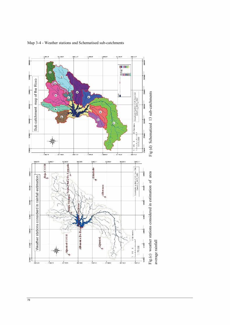
78
Map 3-4 - Weather stations and Schematised sub-catchments
Fi
g (d
) Sc
hem
atiz
ed 1
3 su
b-ca
tchm
ents
Fi
g.(c
) w
eath
er st
atio
ns c
onsi
dere
d in
est
imat
ion
of
area
av
erag
e ra
infa
ll

Analysis of Nutrient Dynamics in Roxo Catchment Using Remote Sensing data and Numerical Modeling
79
Appendix 3 Potential water surface evaporation calculation (sample calculation sheet)
Albureira Do RoxoElevation z 100 mAtmospheric pressure P 100.12 kpaPsychrometric constant γ 0.067 kPaoC-1
Latitude ϕ 37.929 NLongitude 8.080 WAlbedo water α 0.08Wind function coefficient au 1
Date Julian day
Daily mean relative humidity (%)
Daily cum. solar radiation (W/m2)
Daily mean temp. (°C)
Daily mean velocity (m/s)
Max temp. (°C)
Min temp. (°C)
RS
/MJ/m2
/d
RA
/MJ/m2/d
Equation 31 water surface evaporation
9/1/01 244 64 6237 21.5 2.4 31.5 13.8 22.45 33.80 6.529/2/01 245 58 6154 23 0.8 30.7 17.9 22.15 33.59 5.949/3/01 246 58 5832 24.8 2.3 33.3 19.7 21.00 33.38 6.829/4/01 247 62 5777 24.9 1 30.3 19.4 20.80 33.17 5.789/5/01 248 76 5376 23.1 2 27.6 18.0 19.35 32.95 5.219/6/01 249 74 5964 21.4 1.3 24.7 17.4 21.47 32.73 5.199/7/01 250 78 3031 19.6 0.8 30.9 15.5 10.91 32.51 3.189/8/01 251 61 5727 22.8 0.9 33.6 17.4 20.62 32.29 5.759/9/01 252 53 5808 24.5 0.8 33.2 18.3 20.91 32.07 5.96
9/10/01 253 56 5748 23.9 1.2 29.3 16.2 20.69 31.85 5.759/11/01 254 66 5928 21.7 2 26.5 16.1 21.34 31.62 5.659/12/01 255 70 5811 19.8 1.8 26.2 15.5 20.92 31.39 5.259/13/01 256 74 5561 18.2 1.3 28.9 12.5 20.02 31.16 4.849/14/01 257 67 5478 19.7 1.4 28.9 12.3 19.72 30.93 5.089/15/01 258 66 5467 19.9 2.5 31.7 12.7 19.68 30.70 5.749/16/01 259 52 5081 23 0.9 32.3 18.0 18.29 30.47 5.369/17/01 260 59 4700 23.6 1 31.7 17.2 16.92 30.24 4.999/18/01 261 65 5114 21.7 1.3 27.6 15.6 18.41 30.00 4.889/19/01 262 73 4430 19.8 0.9 27.4 15.3 15.95 29.77 4.039/20/01 263 68 4799 20.2 1.3 26.6 15.5 17.28 29.53 4.479/21/01 264 73 3370 19.8 2.3 20.1 15.6 12.13 29.29 3.489/22/01 265 92 1552 17.7 2.4 20.9 15.5 5.59 29.05 1.709/23/01 266 91 2737 18 0.6 22.7 15.9 9.85 28.81 2.309/24/01 267 83 4446 17.9 0.9 22.7 13.8 16.01 28.57 3.479/25/01 268 77 4654 17 1.5 23.4 12.2 16.75 28.33 3.819/26/01 269 72 5135 17.3 1.4 25.7 12.2 18.49 28.09 4.299/27/01 270 63 5039 18.6 0.8 23.5 13.5 18.14 27.85 4.169/28/01 271 76 2971 18.9 1.8 23.2 16.2 10.70 27.61 3.069/29/01 272 82 3250 19.5 2.8 24.6 17.6 11.70 27.37 3.289/30/01 273 88 3202 19.3 0.8 24.7 16.1 11.53 27.13 2.7010/1/01 274 78 4364 18.9 0.8 27.2 15.0 15.71 26.89 3.6610/2/01 275 79 4623 21.3 1.2 25.9 18.4 16.64 26.65 3.9510/3/01 276 83 3174 20.9 0.7 24.6 17.8 11.43 26.40 2.8210/4/01 277 72 3835 18.5 1.8 25.2 12.4 13.81 26.16 3.6410/5/01 278 65 4731 19.2 0.8 24.4 15.6 17.03 25.92 3.9310/6/01 279 87 2251 19.7 0.9 22.1 15.5 8.10 25.68 2.1010/7/01 280 84 3140 17.7 0.9 21.9 14.6 11.30 25.44 2.5710/8/01 281 81 3915 18.3 0.6 21.7 13.6 14.09 25.21 2.9610/9/01 282 80 3067 15.6 0.9 19.0 10.8 11.04 24.97 2.43
10/10/01 283 83 3542 14.2 1.4 20.4 9.5 12.75 24.73 2.6410/11/01 284 78 2525 16.9 2.9 25.7 14.6 9.09 24.49 2.9310/12/01 285 80 2840 20.6 2.9 21.3 17.2 10.22 24.26 2.9210/13/01 286 84 2821 18.2 2.8 22.4 16.3 10.16 24.02 2.6910/14/01 287 84 2913 18 0.8 24.2 13.9 10.49 23.79 2.4310/15/01 288 81 3804 19 0.8 22.4 16.2 13.69 23.56 2.9110/16/01 289 83 3050 17.9 0.5 23.4 14.7 10.98 23.33 2.4210/17/01 290 78 3049 18.8 1.8 23.5 15.6 10.98 23.10 2.84
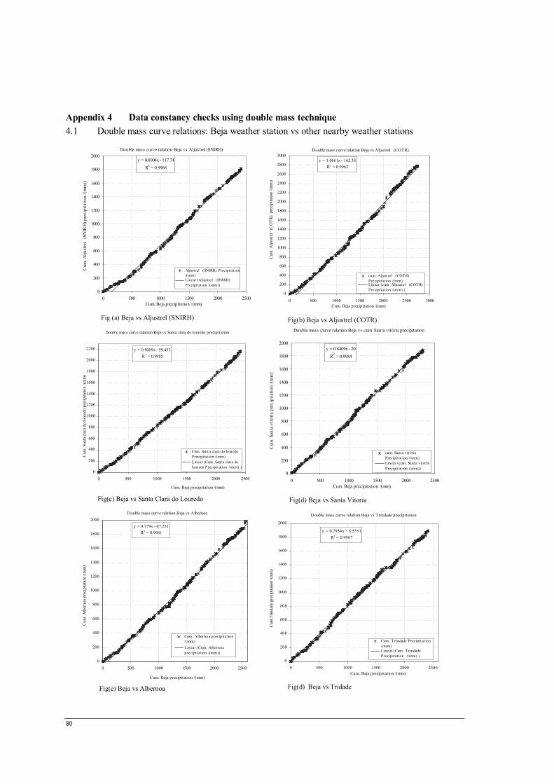
80
Appendix 4 Data constancy checks using double mass technique 4.1 Double mass curve relations: Beja weather station vs other nearby weather stations
Double mass curve ralation Beja vs Aljustrel (SNIRH)
y = 0.8004x - 117.74R2 = 0.9968
0
200
400
600
800
1000
1200
1400
1600
1800
2000
0 500 1000 1500 2000 2500Cum. Beja precipitation /(mm)
Cum
. Alju
stre
l (S
NIR
H) p
reci
pita
tion
/(mm
)) jjj
Aljustrel (SNIRH) Precipitat ion/(mm)Linear (Aljustrel (SNIRH)Precipitat ion /(mm))
Fig (a) Beja vs Aljustrel (SNIRH)
Double mass curve ralation Beja vs Aljustrel (COTR)
y = 1.0661x - 162.38R2 = 0.9962
0
200
400
600
800
1000
1200
1400
1600
1800
2000
2200
2400
2600
2800
3000
0 500 1000 1500 2000 2500 3000Cum. Beja precip itation /(mm)
Cum
. Alju
stre
l (C
OTR
) pr
ecip
itatio
n /(m
m)
jjj
cum. Aljust rel (COTR)Precipitat ion /(mm) Linear (cum. Aljust rel (COTR)Precipitat ion /(mm) )
Fig(b) Beja vs Aljustrel (COTR)
Double mass curve ralation Beja vs Santa clara do louredo precipitation
y = 0.9009x - 59.453R2 = 0.9985
0
200
400
600
800
1000
1200
1400
1600
1800
2000
2200
0 500 1000 1500 2000 2500
Cum. Beja precipitation /(mm)
Cum
. San
ta cl
ara
do lo
ured
o pr
ecip
itatio
n /(m
m)
jjj
jjj
Cum. Santa clara do louredoPrecipitation /(mm) Linear (Cum. Santa clara dolouredo Precipitation /(mm) )
Fig(c) Beja vs Santa Clara do Louredo
Double mass curve ralation Beja vs cum. Santa vitória precipitation
y = 0.8409x - 20R2 = 0.9984
0
200
400
600
800
1000
1200
1400
1600
1800
2000
0 500 1000 1500 2000 2500Cum. Beja precipitation /(mm)
Cum
. San
ta v
itória
pre
cipi
tatio
n /(m
m) jj
jjjj
cum. Santa vitóriaPrecipitat ion /(mm)Linear (cum. Santa vitóriaPrecipitat ion /(mm))
Fig(d) Beja vs Santa Vitoria
Double mass curve ralation Beja vs Albernoa
y = 0.779x - 67.251R2 = 0.9981
0
200
400
600
800
1000
1200
1400
1600
1800
2000
0 500 1000 1500 2000 2500
Cum. Beja precipitation /(mm)
Cum
. Alb
erno
a pr
ecip
itatio
n /(m
m)
jjj
Cum. Albernoa precipitation/(mm)Linear (Cum. Albernoaprecipitation /(mm))
Fig(e) Beja vs Albernoa
Double mass curve ralation Beja vs Trindade precipitation
y = 0.7934x + 8.5351R2 = 0.9967
0
200
400
600
800
1000
1200
1400
1600
1800
2000
0 500 1000 1500 2000 2500Cum. Beja precipitation /(mm)
Cum
.Trin
dade
pre
cipi
tatio
n /(m
m)
jjj
Cum. Trindade Precipitat ion /(mm) Linear (Cum. TrindadePrecipitat ion /(mm) )
Fig(d) Beja vs Tridade

Analysis of Nutrient Dynamics in Roxo Catchment Using Remote Sensing data and Numerical Modeling
81
4.2 Table below shows the slop/gradient of the individual double mass curves shown about in appendix 4.1 and the corresponding coefficient of determination values of the graphs
Precipitation ratio and coefficient of determination
Beja Coefficient of Determination R2
Beja 1.00 1
Aljustrel (SNIRH) 0.80 0.9968
Aljustrel (COTR) 1.07 0.9962Santa Clara do louredo 0.90 0.9985
Santa vitória 0.84 0.9984
Albernoa 0.78 0.9981
Trindade 0.79 0.9967
Albufeira do Roxo 0.89 0.9946
4.2 The Long term precipitation ratios between nearby rainfall stations used in normal ratio method for filling data gaps: Long term precipitation ratios
Beja (COTR)
Aljustrel (SNIRH)
Aljustrel (COTR)
Santa Clara do lured
Santa vitória Albernoa Trindade
Albufeira do Roxo
Beja (COTR) 1.00 1.25 0.94 1.11 1.19 1.28 1.26 1.13
Aljustrel (SNIRH) 0.80 1.00 0.75 0.89 0.95 1.03 1.01 0.90
Aljustrel (COTR) 1.07 1.33 1.00 1.18 1.27 1.37 1.34 1.20
Santa Clara do louredo 0.90 1.13 0.85 1.00 1.07 1.16 1.14 1.02
Santa vitória 0.84 1.05 0.79 0.93 1.00 1.08 1.06 0.95
Albernoa 0.78 0.97 0.73 0.86 0.93 1.00 0.98 0.88
Trindade 0.79 0.99 0.74 0.88 0.94 1.02 1.00 0.90
Albufeira do Roxo 0.89 1.11 0.83 0.98 1.05 1.14 1.12 1.00

82
Appendix 5 Land cover 5.1 Accuracy assessment CORINE land cover classification An accuracy assessment was performed using the ground data and result shows that the overall accuracy is about 90% with a reliability of 85%
5.2 Reclassification results of the individual sub catchment level It is evident that the most common surface type in the Roxo catchment is unpaved, as the catchment dominated by the agriculture. Further in there are few water bodies in the sub catchment and its minor fraction compared to dominant unpaved surfaces. The catchment # 3 is considered to represent the surface runoff directly from the near by area to the reservoir. Moreover the Roxo surface area was not considered in RAM water surface classification as that area was considered in the water balance calculations. Table shows the different percentages of different surface types in each sub-catchment
Sub-catchment Area (km2) Unpaved Other Paved Open Water
1 12.74 98% 0% 2%2 21.96 100% 0% 0%3 19.91 100% 0% 0%4 17.39 90% 10% 0%5 7.27 100% 0% 0%6 18.78 100% 0% 0%7 14.33 98% 2% 0%8 37.13 100% 0% 0%9 35.38 98% 2% 0%
10 39.87 99% 1% 0%11 8.07 100% 0% 0%12 82.58 100% 0% 0%13 24.28 99% 1% 0%
Roxo reservoir area not considered in catchment 13
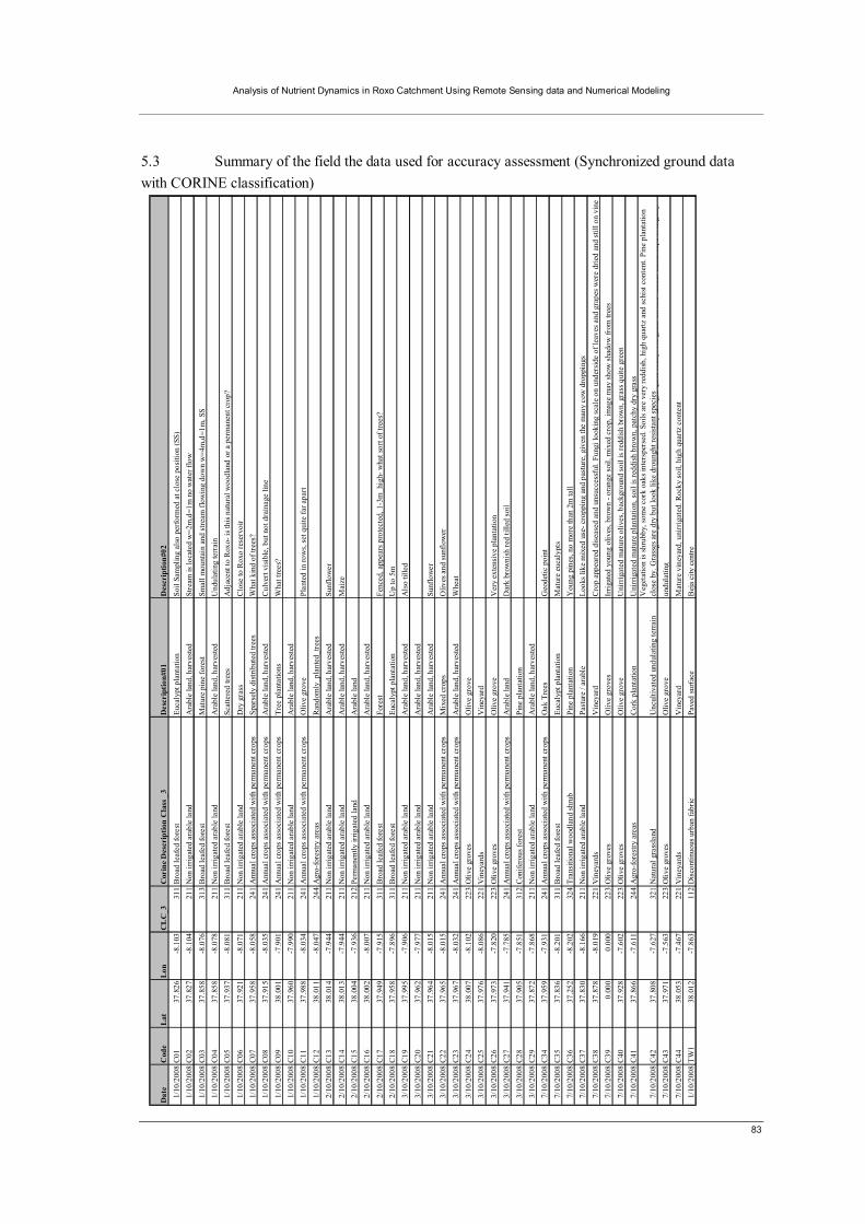
Analysis of Nutrient Dynamics in Roxo Catchment Using Remote Sensing data and Numerical Modeling
83
5.3 Summary of the field the data used for accuracy assessment (Synchronized ground data with CORINE classification)
Dat
eC
ode
Lat
Lon
CL
C_3
Cor
ine
Des
crip
tion
Cla
ss _
3D
escr
iptio
n#01
Des
crip
tion#
021/
10/2
008
C01
37.8
26-8
.103
311
Bro
ad le
afed
fore
stEu
caly
pt p
lant
atio
nSo
il Sa
mpl
ing
also
per
form
ed a
t clo
se p
ositi
on (S
S)1/
10/2
008
C02
37.8
27-8
.104
211
Non
irrig
ated
ara
ble
land
Ara
ble
land
, har
vest
edSt
ream
is lo
cate
d w
=2m
,d=1
m n
o w
ater
flow
1/10
/200
8C
0337
.858
-8.0
7631
3B
road
leaf
ed fo
rest
Mat
ure
pine
fore
stSm
all m
ount
ain
and
stre
am fl
owin
g do
wn
w=4
m,d
=1m
, SS
1/10
/200
8C
0437
.858
-8.0
7821
1N
on ir
rigat
ed a
rabl
e la
ndA
rabl
e la
nd, h
arve
sted
Und
ulat
ing
terr
ain
1/10
/200
8C
0537
.937
-8.0
8131
1B
road
leaf
ed fo
rest
Scat
tere
d tre
esA
djac
ent t
o R
oxo-
is th
is n
atur
al w
oodl
and
or a
per
man
ent c
rop?
1/10
/200
8C
0637
.921
-8.0
7121
1N
on ir
rigat
ed a
rabl
e la
ndD
ry g
rass
Clo
se to
Rox
o re
serv
oir
1/10
/200
8C
0737
.958
-8.0
5824
1A
nnua
l cro
ps a
ssoc
iate
d w
ith p
erm
anen
t cro
psSp
arse
ly d
istri
bute
d tre
esW
hat k
ind
of tr
ees?
1/10
/200
8C
0837
.915
-8.0
3524
1A
nnua
l cro
ps a
ssoc
iate
d w
ith p
erm
anen
t cro
psA
rabl
e la
nd, h
arve
sted
Cul
vert
visi
ble,
but
not
dra
inag
e lin
e1/
10/2
008
C09
38.0
01-7
.901
241
Ann
ual c
rops
ass
ocia
ted
with
per
man
ent c
rops
Tree
pla
ntat
ions
Wha
t tre
es?
1/10
/200
8C
1037
.960
-7.9
9021
1N
on ir
rigat
ed a
rabl
e la
ndA
rabl
e la
nd, h
arve
sted
1/10
/200
8C
1137
.988
-8.0
3424
1A
nnua
l cro
ps a
ssoc
iate
d w
ith p
erm
anen
t cro
psO
live
grov
ePl
ante
d in
row
s, se
t qui
te fa
r apa
rt1/
10/2
008
C12
38.0
11-8
.047
244
Agr
o-fo
rest
ry a
reas
Ran
dom
ly_p
lant
ed_t
rees
2/10
/200
8C
1338
.014
-7.9
4421
1N
on ir
rigat
ed a
rabl
e la
ndA
rabl
e la
nd, h
arve
sted
Sunf
low
er2/
10/2
008
C14
38.0
13-7
.944
211
Non
irrig
ated
ara
ble
land
Ara
ble
land
, har
vest
edM
aize
2/10
/200
8C
1538
.004
-7.9
3621
2Pe
rman
ently
irrig
ated
land
Ara
ble
land
2/10
/200
8C
1638
.002
-8.0
0721
1N
on ir
rigat
ed a
rabl
e la
ndA
rabl
e la
nd, h
arve
sted
2/10
/200
8C
1737
.949
-7.9
1531
1B
road
leaf
ed fo
rest
Fore
stFe
nced
, app
ears
pro
tect
ed, 1
-3m
_hig
h- w
hat s
ort o
f tre
es?
2/10
/200
8C
1837
.958
-7.8
9631
1B
road
leaf
ed fo
rest
Euca
lypt
pla
ntat
ion
Up
to 5
m3/
10/2
008
C19
37.9
95-7
.906
211
Non
irrig
ated
ara
ble
land
Ara
ble
land
, har
vest
edA
lso
tille
d3/
10/2
008
C20
37.9
62-7
.977
211
Non
irrig
ated
ara
ble
land
Ara
ble
land
, har
vest
ed3/
10/2
008
C21
37.9
64-8
.015
211
Non
irrig
ated
ara
ble
land
Ara
ble
land
, har
vest
edSu
nflo
wer
3/10
/200
8C
2237
.965
-8.0
1524
1A
nnua
l cro
ps a
ssoc
iate
d w
ith p
erm
anen
t cro
psM
ixed
cro
psO
lives
and
sun
flow
er3/
10/2
008
C23
37.9
67-8
.032
241
Ann
ual c
rops
ass
ocia
ted
with
per
man
ent c
rops
Ara
ble
land
, har
vest
edW
heat
3/10
/200
8C
2438
.007
-8.1
0222
3O
live
grov
esO
live
grov
e3/
10/2
008
C25
37.9
76-8
.086
221
Vin
eyar
dsV
iney
ard
3/10
/200
8C
2637
.973
-7.8
2022
3O
live
grov
es
Oliv
e gr
ove
Ver
y ex
tens
ive
plan
tatio
n3/
10/2
008
C27
37.9
41-7
.785
241
Ann
ual c
rops
ass
ocia
ted
with
per
man
ent c
rops
Ara
ble
land
Dar
k br
owni
sh re
d til
led
soil
3/10
/200
8C
2837
.905
-7.8
5131
2C
onife
rous
fore
st
Pine
pla
ntat
ion
3/10
/200
8C
2937
.872
-7.8
6821
1N
on ir
rigat
ed a
rabl
e la
ndA
rabl
e la
nd, h
arve
sted
7/10
/200
8C
3437
.959
-7.9
3124
1A
nnua
l cro
ps a
ssoc
iate
d w
ith p
erm
anen
t cro
ps
Oak
Tre
esG
eode
tic p
oint
7/10
/200
8C
3537
.836
-8.2
0131
1B
road
leaf
ed fo
rest
Euca
lypt
pla
ntat
ion
Mat
ure
euca
lypt
s7/
10/2
008
C36
37.2
52-8
.202
324
Tran
sitio
nal w
oodl
and
shru
bPi
ne p
lant
atio
nY
oung
pin
es, n
o m
ore
than
2m
tall
7/10
/200
8C
3737
.830
-8.1
6621
1N
on ir
rigat
ed a
rabl
e la
ndPa
stur
e / a
rabl
eLo
oks
like
mix
ed u
se- c
ropp
ing
and
past
ure,
giv
en th
e m
any
cow
dro
ppin
gs7/
10/2
008
C38
37.8
78-8
.019
221
Vin
eyar
dsV
iney
ard
Cro
p ap
pear
ed d
isea
sed
and
unsu
cces
sful
. Fun
gi lo
okin
g sc
ale
on u
nder
side
of l
eave
s and
gra
pes w
ere
drie
d an
d st
ill o
n vi
ne7/
10/2
008
C39
0.00
00.
000
223
Oliv
e gr
oves
Oliv
e gr
oves
Irrig
ated
you
ng o
lives
, bro
wn
- ora
nge
soil,
mix
ed c
rop,
imag
e m
ay sh
ow s
hado
w fr
om tr
ees
7/10
/200
8C
4037
.928
-7.6
0222
3O
live
grov
esO
live
grov
eU
nirr
igat
ed m
atur
e ol
ives
, bac
kgro
und
soil
is re
ddis
h br
own,
gra
ss q
uite
gre
en7/
10/2
008
C41
37.8
66-7
.611
244
Agr
o-fo
rest
ry a
reas
Cor
k pl
anta
tion
Uni
rrig
ated
mat
ure
plan
tatio
n, s
oil i
s red
dish
bro
wn,
pat
chy
dry
gras
s
7/10
/200
8C
4237
.808
-7.6
2732
1N
atur
al g
rass
land
Unc
ultiv
ated
und
ulat
ing
terr
ain
Veg
etat
ion
is sh
rubb
y, s
ome
cork
oak
s int
ersp
erse
d. S
oils
are
ver
y re
ddis
h, h
igh
quar
tz a
nd s
chis
t con
tent
. Pin
e pl
anta
tion
clos
e by
. Gra
sses
are
dry
but
look
like
dro
ungh
t res
ista
nt s
peci
es7/
10/2
008
C43
37.9
71-7
.563
223
Oliv
e gr
oves
Oliv
e gr
ove
Mat
ure
and
irrig
ated
gro
ve. S
oil a
ppea
rs d
ark
and
loam
y th
ough
t qui
te ro
cky.
No
gras
s on
soil
tille
d. L
ands
cape
is sl
ight
ly
undu
latin
g7/
10/2
008
C44
38.0
53-7
.467
221
Vin
eyar
dsV
iney
ard
Mat
ure
vine
yard
, uni
rrig
ated
. Roc
ky so
il, h
igh
quar
tz c
onte
nt1/
10/2
008
TW
138
.012
-7.8
6311
2D
isco
ntin
uous
urb
an fa
bric
Pave
d su
rfac
eB
eja
city
cen
tre

84
Appendix 6 Data for crop evapotranspiration estimates Growing Seasons
Crop Type Init.(Lini) Dev.(Ldev) Mid.(Lmid) Late.(Llate) Total Planting date
Sunflower 25 35 45 25 130 April
Winter Wheat 30 140 40 30 240 November
Maize (sweet) 20 25 25 10 80 May/June
Growing-Olives 30 90 60 90 270 March
Grapes 30 60 40 80 210 April
Olives 30 90 60 90 270 March
Crop factors at different growth stages
SunflowerWinter Wheat
Maize (sweet)
Growing-Olives Grapes Olives Bare Soils
Forests- Coniferous
Grazing Pasture
Kc, ini 0.45 0.7 0.45 0.65 0.3 0.65 0.45 1 0.3
Kc, mid 1.15 1.15 1.15 0.7 0.7 0.45 0.45 1 0.75
Kc, end 0.35 0.25 1.05 0.7 0.45 0.65 0.45 1 0.75
Max crop height/(m) 2 1 1.5 3 to 5 1.5-2 10 0.1
Crop type and crop factors at different growth stages
Stage
Percentages of individual land cover types at each sub catchment
1 2 3 4 5 6 7 8 9 10 11 12 13
112 Discontinuous urban fabric 10.2 1.95 1.5 0.66 0.06
211 Non-irrigated arable land 63.78 37.72 79.45 86.96 88.87 60.81 68.87 77.57 82.32 64.04 59.82 70.41 47.96
212 Permanently irrigated land 1.64 4.37 5.13 1.34 9 3.89 3.28 0.59 17.24
221 Vineyards 0.03
223 Olive groves 10.41 6.32 0.57 0.58 2.7 4.74 0.49 0.71
241Annual crops associated with permanent crops 1.58 1.51 2.13 18.44 26.51 2.43 8.71 16.98 22.45 0.32 3.66
242 Complex cultivation patterns 0.7 1.39
243Land principally occupied by agriculture, with significant areas of natural vegetation 0.94 1.37 0.05
244 Agro-forestry areas 27.96 23.05 2.99 11.29 13.47 12.99 18.22 9.8
311 Broad-leaved forest 3.31 33.54 0.05 1.9 10.14 0.14
313 Mixed forest 1.17
321 Natural grasslands 0.15 0.43 1.72 2.07 0.15 0.23 14.51
324 Transitional woodland-shrub 0.62
512 Water bodies 2.36 0.78 21.78100 100 100 100 100 100 100 100 100 100 100 100 100
Sub catchment land cover percentage (%)
TypeCORINE
Code

Analysis of Nutrient Dynamics in Roxo Catchment Using Remote Sensing data and Numerical Modeling
85
Appendix 7 Roxo Stage Volume curve (Mannaerts , 2006)
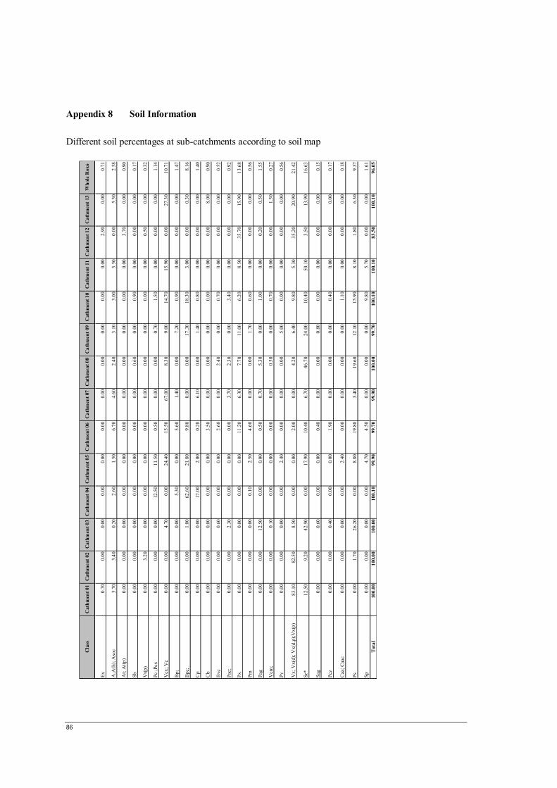
86
Appendix 8 Soil Information Different soil percentages at sub-catchments according to soil map
Cla
ssC
athm
ent 0
1C
athm
ent 0
2C
athm
ent 0
3C
athm
ent 0
4C
athm
ent 0
5C
athm
ent 0
6C
athm
ent 0
7C
athm
ent 0
8C
athm
ent 0
9C
athm
ent 1
0C
athm
ent 1
1C
athm
ent 1
2C
athm
ent 1
3W
hole
Rox
o
Ex0.
700.
000.
000.
000.
000.
000.
000.
000.
000.
000.
002.
900.
000.
71
A;A
(h);
Aso
c3.
703.
400.
202.
601.
506.
704.
602.
403.
103.
003.
500.
005.
502.
58
At;
At(p
)0.
000.
000.
000.
000.
000.
000.
000.
000.
000.
000.
003.
700.
000.
90
Sb0.
000.
000.
000.
000.
000.
000.
000.
600.
000.
900.
000.
000.
000.
17
Vt(p
)0.
003.
200.
000.
000.
000.
000.
000.
000.
000.
000.
000.
500.
000.
32
Pc ;P
cx0.
000.
000.
0012
.50
11.5
00.
500.
000.
000.
701.
500.
000.
000.
001.
14
Vcx
; Vc
0.00
0.00
4.70
0.00
24.4
015
.50
67.0
08.
309.
0014
.70
15.9
00.
0027
.30
10.7
1
Bp;
0.00
0.00
0.00
5.30
0.00
5.60
1.40
0.00
7.20
0.90
0.00
0.00
0.00
1.47
Bpc
;0.
000.
001.
0062
.60
21.8
09.
800.
000.
0017
.30
18.3
03.
000.
000.
308.
16
Cp
0.00
0.00
0.00
17.0
02.
000.
206.
100.
001.
400.
800.
000.
000.
001.
40
Cb
0.00
0.00
0.00
0.00
0.00
3.50
0.00
0.00
0.00
0.00
0.00
0.00
8.00
0.90
Bvc
0.00
0.00
0.60
0.00
0.00
2.60
0.00
2.40
0.00
0.70
0.00
0.00
0.00
0.52
Pac;
0.00
0.00
2.30
0.00
0.00
0.00
3.70
2.30
0.00
3.40
0.00
0.00
0.00
0.92
Px0.
000.
000.
000.
000.
0011
.20
6.30
7.70
11.0
06.
208.
5035
.70
15.9
013
.68
Pm0.
000.
000.
000.
102.
504.
600.
000.
001.
700.
600.
000.
000.
000.
56
Pag
0.00
0.00
12.5
00.
000.
000.
500.
705.
300.
001.
000.
000.
200.
501.
55
Vcm
;0.
000.
000.
100.
000.
000.
000.
000.
500.
000.
700.
000.
001.
500.
27
Pv0.
000.
000.
000.
002.
400.
000.
000.
005.
000.
000.
000.
000.
000.
56
Vx;
Vx(
d); V
x(d,
p);V
x(p)
83.1
082
.50
8.50
0.00
0.00
2.00
0.00
4.20
6.40
9.80
5.30
35.2
020
.90
21.4
2
Sr*
12.5
09.
2042
.90
0.00
17.9
010
.40
6.70
46.7
024
.00
10.4
050
.10
3.50
13.9
016
.63
Sag
0.00
0.00
0.60
0.00
0.00
0.40
0.00
0.00
0.80
0.00
0.00
0.00
0.00
0.15
Pcz
0.00
0.00
0.40
0.00
0.00
1.90
0.00
0.00
0.00
0.40
0.00
0.00
0.00
0.17
Caa
; Caa
c0.
000.
000.
000.
002.
400.
000.
000.
000.
001.
100.
000.
000.
000.
18
Ps0.
001.
7026
.20
0.00
8.80
19.8
03.
4019
.60
12.1
015
.90
8.10
1.80
6.30
9.37
Sp0.
000.
000.
000.
004.
704.
500.
000.
000.
009.
805.
700.
000.
001.
61To
tal
100.
0010
0.00
100.
0010
0.10
99.9
099
.70
99.9
010
0.00
99.7
010
0.10
100.
1083
.50
100.
1096
.05

Analysis of Nutrient Dynamics in Roxo Catchment Using Remote Sensing data and Numerical Modeling
87
Summary of the soil properties
S
ome
of th
e so
il da
ta c
olle
cted
from
the
liter
atur
e
22.
74.
2In
itial
Con
stan
t
Bro
wn
Cal
care
ous S
oils
Brow
n C
alc.
S. o
f Sub
-hum
ic a
nd s
emi a
rid
clim
ates
Pc ;P
cx46
.65
39.3
031
.20
23.2
55.
8025
.40
0.90
1.00
Red
Cal
care
ous
Soils
Red
Cal
c.S.
of S
ub-H
um a
nd S
emi A
rid
Clim
ates
Vcx
; Vc
47.8
748
.60
24.7
727
.94
15.4
39.
341.
552.
88
Non
Cal
care
ous B
lack
Bar
ros
Bp
51.9
245
.53
39.0
031
.27
18.4
720
.53
0.63
0.70
Cal
care
ous
Bla
ck B
arro
s St
rong
ly
deca
rbon
ated
Bpc
50.9
051
.00
40.8
035
.55
20.4
020
.40
2.11
1.68
Cal
care
ous
Bla
ck B
arro
s Sl
ight
ly
deca
rbon
ated
Cp
47.7
047
.28
41.4
837
.18
20.3
521
.13
0.45
0.75
Non
Cal
care
ous D
ark
Red
dish
Bro
wn
Barr
osC
b45
.63
38.6
523
.73
18.7
310
.73
13.0
012
.91
9.01
Cal
care
ous
Dar
k R
eddi
sh B
row
n B
arro
s St
rong
ly D
ecar
bona
ted
Bvc
52.7
650
.89
25.3
328
.49
17.4
87.
853.
595.
93
Brow
n M
edit.
S.fr
om c
alca
reou
s roc
ksPa
c43
.80
35.8
825
.38
21.0
09.
6815
.95
3.32
2.93
Brow
n M
edit.
S.fr
om n
on-c
alca
reou
s roc
ks -
Nor
mal
sPx
38.6
730
.17
22.2
620
.24
9.12
13.1
40.
580.
80
Brow
n M
edit.
S.fr
om n
on-c
alca
reou
s roc
ks -
Para
Bar
ros
Pm43
.73
37.4
528
.18
23.1
59.
9318
.26
6.92
4.80
Red
-Yel
. Med
it.S.
from
cal
care
ous r
ocks
- Pa
ra B
arro
sV
cm44
.87
37.2
321
.72
17.4
713
.06
8.66
0.00
0.91
Red
-Yel
. Med
it.S.
from
non
-cal
care
ous
rock
s - N
orm
als
Pv50
.27
45.6
838
.45
32.7
016
.64
21.8
10.
350.
48
Red
-Yel
. Med
it.S.
from
non
-cal
care
ous
rock
s - N
orm
als
Vx;
Vx(
d);
Vx(
d,p)
;Vx(
p)52
.00
52.0
537
.80
36.7
514
.29
23.5
20.
900.
80
Red
-Yel
. Med
it.S.
from
non
-cal
care
ous
rock
s - w
ith p
linth
itic
mat
eria
lsSr
*41
.87
32.4
221
.80
16.6
08.
9313
.06
14.3
310
.75
With
Elu
vial
Hor
izon
Plan
osol
s w
ith E
luvi
al H
oris
onPs
41.3
835
.53
23.4
817
.03
10.9
812
.47
7.80
4.60
Hyd
rom
orph
ic
Soils
Barr
os
Dar
k R
eddi
sh B
row
n B
orro
s
Bla
ck B
arro
s
Less
ives
Soi
ls
(Not
Stro
ngly
U
nsat
urat
ed)
Bro
wn
Med
iterr
anea
n So
ils
Red
-Yel
low
M
edite
rran
ean
Soils
Cal
care
ous
Soils
Perm
eabi
lity
cm/h
Soil
Typ
e II
Ava
ilabl
e w
ater
%
PFM
ax. w
ater
H
oldi
ng
Cap
acity
%Po
rosi
ty %
Not
atio
nD
etai
led
Typ
e IV
Soil
type
I
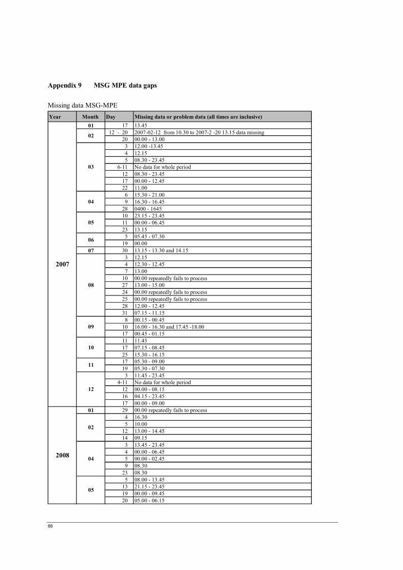
88
Appendix 9 MSG MPE data gaps Missing data MSG-MPE Year Month Day Missing data or problem data (all times are inclusive)
01 17 13.4512 - 20 2007-02-12 from 10.30 to 2007-2 -20 13.15 data missing
20 00.00 - 13.00 3 12.00 -13.454 12.155 08.30 - 23.45
6-11 No data for whole period12 08.30 - 23.4517 00.00 - 12.4522 11.006 15.30 - 21.00 9 16.30 - 16.45
28 0400 - 1645 10 23.15 - 23.4511 00.00 - 06.4523 13.155 05.45 - 07.30
19 00.0007 30 13.15 - 13.30 and 14.15
3 12.15 4 12.30 - 12.457 13.00
10 00.00 repeatedly fails to process27 13.00 - 15.0024 00.00 repeatedly fails to process25 00.00 repeatedly fails to process28 12.00 - 12.4531 07.15 - 11.158 00.15 - 00.45
10 16.00 - 16.30 and 17.45 -18.00 17 00.45 - 01.15 11 11.4517 07.15 - 08.4525 15.30 - 16.15 17 05.30 - 09.0019 05.30 - 07.303 11.45 - 23.45
4-11 No data for whole period12 00.00 - 08.1516 04.15 - 23.4517 00.00 - 09.00
01 29 00.00 repeatedly fails to process4 16.305 10.00
12 13.00 - 14.4514 09.153 13.45 - 23.454 00.00 - 06.455 00.00 - 02.459 08.30
23 08.305 08.00 - 13.45
13 21.15 - 23.4519 00.00 - 09.45 20 05.00 - 06.15
11
02
03
04
05
2008
06
08
09
10
12
02
04
05
2007
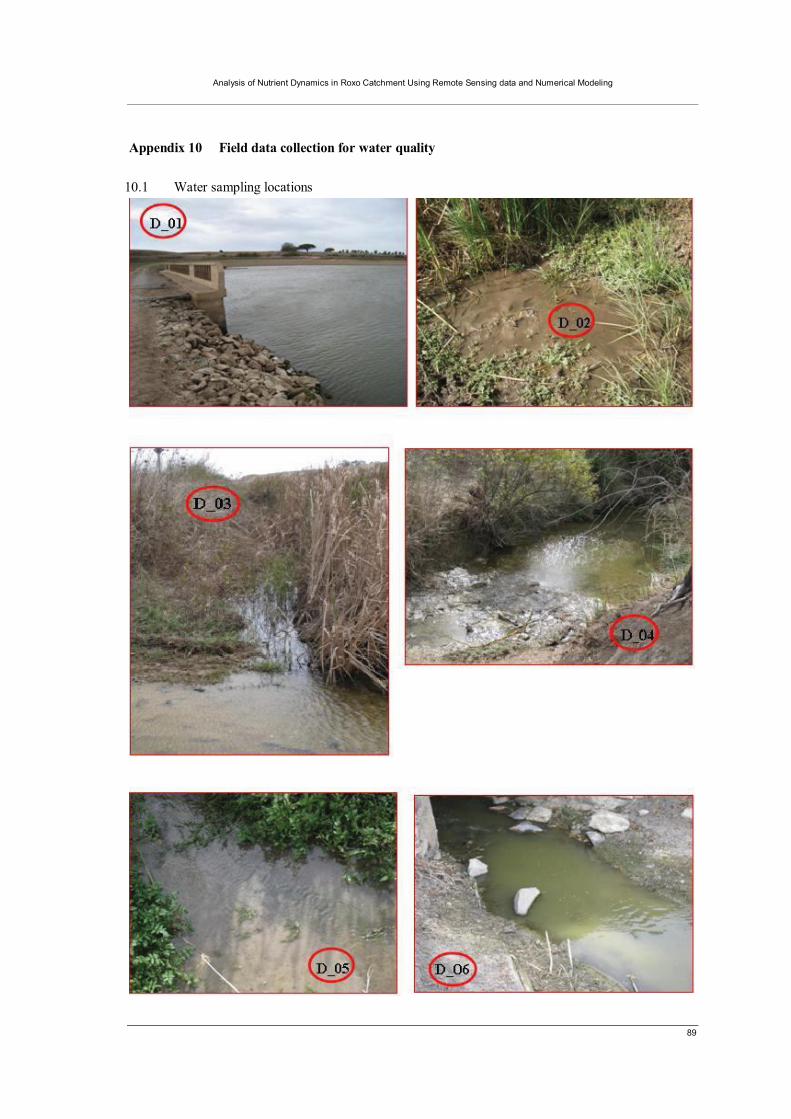
Analysis of Nutrient Dynamics in Roxo Catchment Using Remote Sensing data and Numerical Modeling
89
Appendix 10 Field data collection for water quality 10.1 Water sampling locations
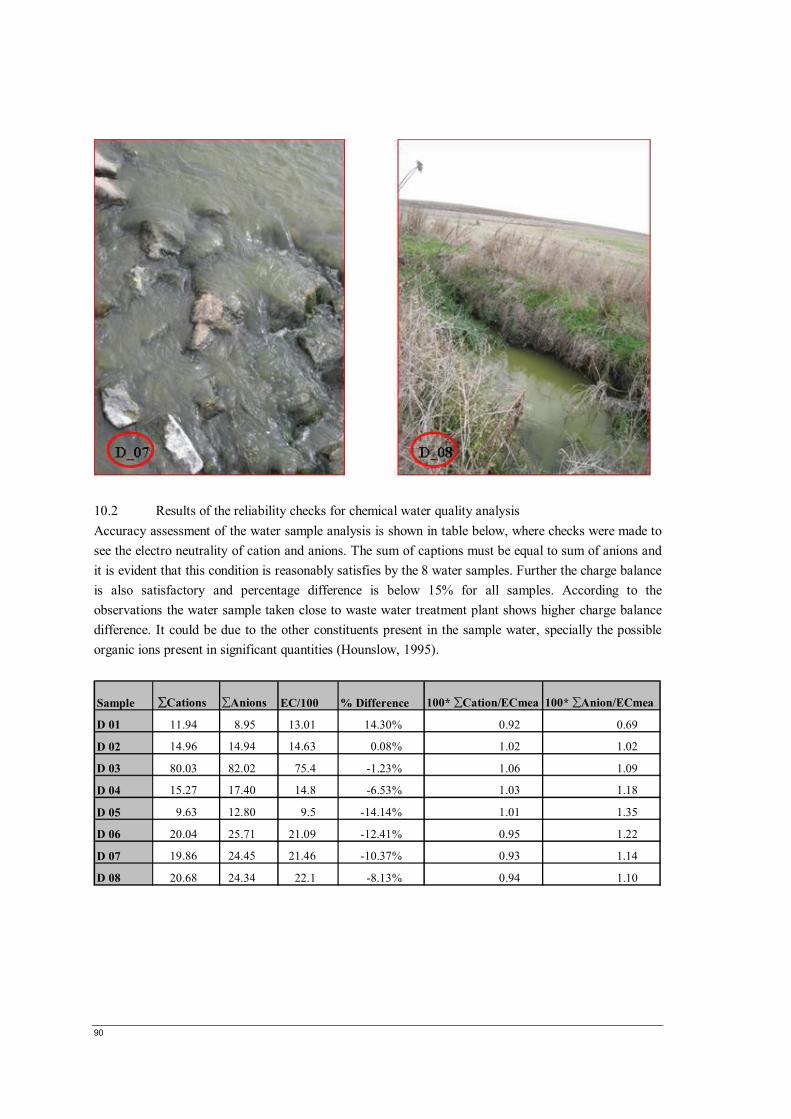
90
10.2 Results of the reliability checks for chemical water quality analysis Accuracy assessment of the water sample analysis is shown in table below, where checks were made to see the electro neutrality of cation and anions. The sum of captions must be equal to sum of anions and it is evident that this condition is reasonably satisfies by the 8 water samples. Further the charge balance is also satisfactory and percentage difference is below 15% for all samples. According to the observations the water sample taken close to waste water treatment plant shows higher charge balance difference. It could be due to the other constituents present in the sample water, specially the possible organic ions present in significant quantities (Hounslow, 1995).
Sample ∑∑Cations ∑Anions EC/100 % Difference 100* ∑Cation/ECmea 100* ∑Anion/ECmea
D 01 11.94 8.95 13.01 14.30% 0.92 0.69
D 02 14.96 14.94 14.63 0.08% 1.02 1.02
D 03 80.03 82.02 75.4 -1.23% 1.06 1.09
D 04 15.27 17.40 14.8 -6.53% 1.03 1.18
D 05 9.63 12.80 9.5 -14.14% 1.01 1.35
D 06 20.04 25.71 21.09 -12.41% 0.95 1.22
D 07 19.86 24.45 21.46 -10.37% 0.93 1.14
D 08 20.68 24.34 22.1 -8.13% 0.94 1.10

Analysis of Nutrient Dynamics in Roxo Catchment Using Remote Sensing data and Numerical Modeling
91
Appendix 11 Salt dilution gauging Field observations (37o,57’ 34.5” N, 7o 58’ 33.8” W) The salt (NaCl) quantity used in the test is 400 g and the distance between salt application and EC measuring point is 20 m.
Time (s)EC
(μs/cm) Time (s)EC
(μs/cm) Time (s)EC
(μs/cm)0 1559 220 3370 380 1982
10 1559 230 3340 390 195220 1559 240 3230 400 192330 1556 250 3070 410 188740 1556 260 2960 420 187350 1555 270 2800 440 183760 1554 280 2660 450 182070 1553 290 2540 460 179680 1551 300 2510 470 177890 1549 310 2410 480 1758
120 1547 320 2350 490 1745160 2151 330 2280 500 1735170 2700 340 2210 510 1724180 2970 350 2160 520 1731190 3190 360 2090 640 1637200 3370 370 2030 700 1611210 3450
Graph displaying the variation of electrical conductivity after introducing the NaCl upstream. The area under the graph is equivalent to the equation [7.1] and the area was calculated using the trapezoidal rule. The flow was calculated subsequently and was found to equal to 0.12 m3/sec.
Electrical conductivity measurement at stream section (μS/cm) with time
1500
1700
1900
2100
2300
2500
2700
2900
3100
3300
3500
0 100 200 300 400 500 600 700
Time in Seconds /(s)
Elec
trica
l con
duct
ivity
μS
/cm
jj
jjj
Electrical conductivity (ms/cm)
( )( )∫∞
−0
,1t
btx CC
[ 0.1]
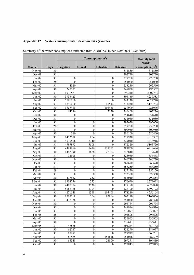
92
Appendix 12 Water consumption/abstraction data (sample) Summary of the water consumptions extracted from ABROXO (since Nov 2001 –Oct 2005)
Irrigation Animal Industrial DrinkingNov-01 30 311850 311850Dec-01 31 302770 302770Jan-02 31 0 0 279750 279750Feb-02 28 0 0 251060 251060Mar-02 31 4320 0 258240 262560Apr-02 30 247707 0 248850 496557
May-02 31 1911573 0 296210 2207783Jun-02 30 3933423 0 304160 4237583Jul-02 31 5681610 0 343130 6024740
Aug-02 31 4796010 41544 333230 5170784Sep-02 30 1357488 108468 259090 1725046Oct-02 31 64296 2520 340460 407276
Nov-02 30 0 0 354640 354640Dec-02 31 0 0 331080 331080Jan-03 31 0 0 0 295650 295650Feb-03 28 0 0 0 259280 259280Mar-03 31 0 0 0 309950 309950Apr-03 30 360 0 0 280100 280460
May-03 31 1472508 864 0 339930 1813302Jun-03 30 4015566 2340 0 329010 4346916Jul-03 31 4787892 5508 0 372320 5165720
Aug-03 31 4389966 1476 139392 387860 4918694Sep-03 30 1442790 3888 28152 342840 1817670Oct-03 31 32508 0 0 323960 356468
Nov-03 30 0 0 0 340730 340730Dec-03 31 0 0 0 368670 368670Jan-04 31 0 0 0 366250 366250Feb-04 29 0 0 0 355150 355150Mar-04 31 0 0 0 372350 372350Apr-04 30 437562 252 0 353040 790854
May-04 31 1908756 252 0 370690 2279698Jun-04 30 4407174 3536 0 419180 4829890Jul-04 31 5968188 2304 0 428700 6399192
Aug-04 31 4271148 1368 105408 378240 4756164Sep-04 30 1705518 504 95904 365110 2167036Oct-04 31 437328 0 0 351050 788378
Nov-04 30 0 0 0 296774 296774Dec-04 31 0 0 0 349916 349916Jan-05 31 0 0 0 335097 335097Feb-05 28 0 0 0 294696 294696Mar-05 31 0 0 0 336963 336963Apr-05 30 0 0 0 336611 336611
May-05 31 48888 0 0 301274 350162Jun-05 30 62787 0 0 321290 384077Jul-05 31 60282 0 0 299919 360201
Aug-05 31 81585 0 153648 254076 489309Sep-05 30 66348 0 28800 299271 394419Oct-05 31 0 0 0 275843 275843
Mon/Yr Days
Consumption (m3) Monthly total water
consumption (m3)

Analysis of Nutrient Dynamics in Roxo Catchment Using Remote Sensing data and Numerical Modeling
93
Appendix 13 Collected ground control points for Geo-referencing
10/3/2008 A01 38.006 -7.869 258 Opposite to Beja Porque hotel , inside the round about
10/3/2008 A02 37.989 -7.916 222 Ervidel & Beja junction
10/3/2008 A03 37.965 -8.023 166Mina da Juliana junction,surroundings have residential buildings, opposite road leads to beja
10/3/2008 A04 37.967 -8.031 147 Mombeja junction
10/3/2008 A05 37.967 -8.082 159 Fourway junction, (Beja, Ervidel, Adejas, Aljustrel)
10/3/2008 A06 38.057 -8.120 137 Lisbon junction, mercado area
10/3/2008 A07 37.859 -8.086 161 Barragem Roxo junction, with open fields around
10/3/2008 A08 37.948 -8.096 142 Cotre VTE anesl surrounded by cultivated land
10/3/2008 A09 38.003 -7.866 251 Round about opposite to McDonalds
10/3/2008 A10 37.978 -7.827 230 Beja, Salvada junction, opposite to Quintos junction
10/3/2008 A11 37.941 -7.784 209 Round about
10/3/2008 A12 37.907 -7.869 174 Accesso local junction
10/3/2008 A13 37.911 -7.872 171 T junction
10/3/2008 A14 37.893 -7.896 171 Beja Evora Ourique Castro verde junction
10/3/2008 A15 37.972 -7.874 207 Penedo Gordo Junction, 4 way junction
DescriptionLatitude LongitudeElevation
(m)Date Point
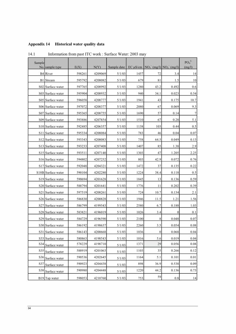
94
Appendix 14 Historical water quality data
14.1 Information from past ITC work : Surface Water: 2003 may
Sample No. sample type E(X) N(Y) Sample date EC μS/cm NO3
- (mg/l) NO2- (mg/l)
PO43-
(mg/l)
B4 River 598261 4209069 5/1/03 1457 72 3.4 14
B1 Stream 595792 4208082 5/1/03 679 81 1.5 10
S02 Surface water 597765 4208992 5/1/03 1280 43.2 0.492 0.6
S03 Surface water 595904 4208932 5/1/03 940 34.1 0.023 0.54
S05 Surface water 596058 4208777 5/1/03 1941 43 0.175 10.7
S06 Surface water 597072 4208377 5/1/03 2080 67 0.069 9.3
S07 Surface water 595365 4208755 5/1/03 1690 57 0.14 7
S09 Surface water 593886 4207854 5/1/03 1510 67 0.28 5.1
S10 Surface water 592485 4206357 5/1/03 1138 103 0.44 0.5
S11 Surface water 595334 4208084 5/1/03 783 46 0.04 0.07
S12 Surface water 593343 4208083 5/1/03 758 64.5 0.049 0.13
S13 Surface water 593233 4207408 5/1/03 1407 85 1.38 2.9
S15 Surface water 593511 4207140 5/1/03 1303 47 1.205 2.25
S16 Surface water 594802 4207252 5/1/03 803 42.9 0.072 0.76
S17 Surface water 592048 4204321 5/1/03 1472 37 0.135 0.22
S18B Surface water 590104 4202280 5/1/03 1224 38.4 0.118 0.5
S19 Surface water 590694 4201628 5/1/03 1845 13 0.136 0.59
S20 Surface water 588794 4201641 5/1/03 1776 11 0.202 0.39
S21 Surface water 597519 4208261 5/1/03 724 10.7 0.134 2.1
S26 Surface water 586830 4200828 5/1/03 1946 11.5 1.21 1.56
S27 Surface water 586799 4199543 5/1/03 2580 6.7 0.188 1.03
S28 Surface water 583821 4196019 5/1/03 1026 3.4 0 0.1
S29 Surface water 584729 4196590 5/1/03 2100 8 0.048 0.07
S30 Surface water 586192 4198637 5/1/03 2260 3.5 0.054 0.08
S31 Surface water 586143 4200668 5/1/03 1036 0 0.068 0.04
S33 Surface water 580863 4198543 5/1/03 1016 5.6 0.019 0.04S34 Surface water 578229 4198710 5/1/03 1371 29 0.056 0.08
S35 Surface water 588919 4201063 5/1/03 1103 35 0.266 0.12
S36 Surface water 590536 4202645 5/1/03 1164 5.1 0.101 0.01
S37 Surface water 590923 4204438 5/1/03 898 36.9 0.538 0.09
S38 Surface water 590980 4204448 5/1/03 1220 44.2 0.136 0.73
B19 Tap water 598053 4210760 5/1/03 753 59 0.8 14

Analysis of Nutrient Dynamics in Roxo Catchment Using Remote Sensing data and Numerical Modeling
95
14.2 Water quality information collected from EMAS The sampling location is the Roxo reservoir and the concentration data for the Roxo waters are available since Jan 2005 till Jan 2008.
ID-RQAData de colheita Nitratos
Fósforo total Fosfatos
Azoto Kjedahl
Azoto amoniacal
Amoníaco não ionizado Nitritos
5210 11-01-2005 5.09 0.054 <0,023 1.13 0.26 0.0119 0.027 5210 09-02-2005 0.93 0.064 0.034 0 0.26 0.0212 0.032 5210 08-03-2005 1.24 0.06 0.121 1.45 0.26 0.0826 0.037 5210 05-04-2005 1.28 0.369 0.042 0 0.16 0.0156 0.034 5210 03-05-2005 0.58 0.031 0.032 0.74 0.11 0.0012 0.017 5210 31-05-2005 2.39 0.059 0.036 0 0.04 0.0079 0.001 5210 27-06-2005 0.56 0.057 0 1.24 0.16 0.0343 0.003 5210 26-07-2005 0.59 0.046 0.026 0 0.11 0.0042 0.003 5210 06-09-2005 0.63 0.054 <0,023 1.1 0.04 0.0377 0.01 5210 03-10-2005 1.11 0.09 0.023 0 0.15 0.0307 0.001 5210 02-11-2005 0.8 0.123 0.037 1.49 0.15 0.0251 0.026 5210 29-11-2005 3.01 0.135 0.061 0 0.42 0.3519 0.065 5210 10-01-2006 3.19 0.042 0.037 1.03 0.49 0.0006 0.072 5210 07-02-2006 3.19 0.029 <0,023 0 <0,04 0.00338 <0,001 5210 07-03-2006 2.97 0.039 0.025 0.41 0.05 0.0201 0.003 5210 04-04-2006 0.97 0.045 0.029 0 0.07 0.0173 0.034 5210 02-05-2006 1.02 0.049 0.027 0.83 0.13 0.0264 0.011 5210 30-05-2006 0.04 0.047 <0,023 0 0.18 0.04286 0.002 5210 26-06-2006 1.2 0.069 0.045 0.76 0.17 0.0226 <0,001 5210 26-07-2006 <0,09 0.125 0.04 0 0.11 0.0116 0.001 5210 05-09-2006 0.13 0.159 0.059 1.16 0.1 0.0205 0.001 5210 02-10-2006 <0,09 0.077 0.115 0 0.14 0.0048 0.003 5210 30-10-2006 <2,00 0.069 <0,023 1.26 0.15 0.0186 0.014 5210 28-11-2006 <2,00 0.059 0.113 0 0.42 0.0096 0.155 5210 02-01-2007 3.8 0.09 0.05 0.78 0.12 0.0109 0.02 5210 30-01-2007 3.1 0.049 0.035 0 0.19 0.0066 0.062 5210 27-02-2007 3.2 0.035 <0,023 0.73 0.15 0.005 0.054 5210 27-03-2007 <2,00 0.037 0.033 0 0.23 0.0071 0.065 5210 02-05-2007 <2,00 0.038 <0,023 0.51 0.06 0.0304 0.08 5210 29-05-2007 <2,00 0.499 <0,023 0 <0,04 0.0013 0.012 5210 25-06-2007 <2,00 0.033 <0,023 1.3 <0,04 0.0019 0.008 5210 23-07-2007 <2,00 0.026 <0,023 0 <0,04 0.0001 0.003 5210 11-09-2007 <2,00 0.044 0.023 0.94 <0,08 0.002 0.004 5210 01-10-2007 3.9 0.039 <0,023 0 <0,08 0.0009 <0,002 5210 29-10-2007 <2,00 0.204 <0,023 0.59 0.12 0.0026 0.019 5210 27-11-2007 <2,00 0.066 <0,023 0 0.36 0.00138 0.123 5210 02-01-2008 <2,00 0.03 <0,023 0.45 0.22 0.0096 0.072
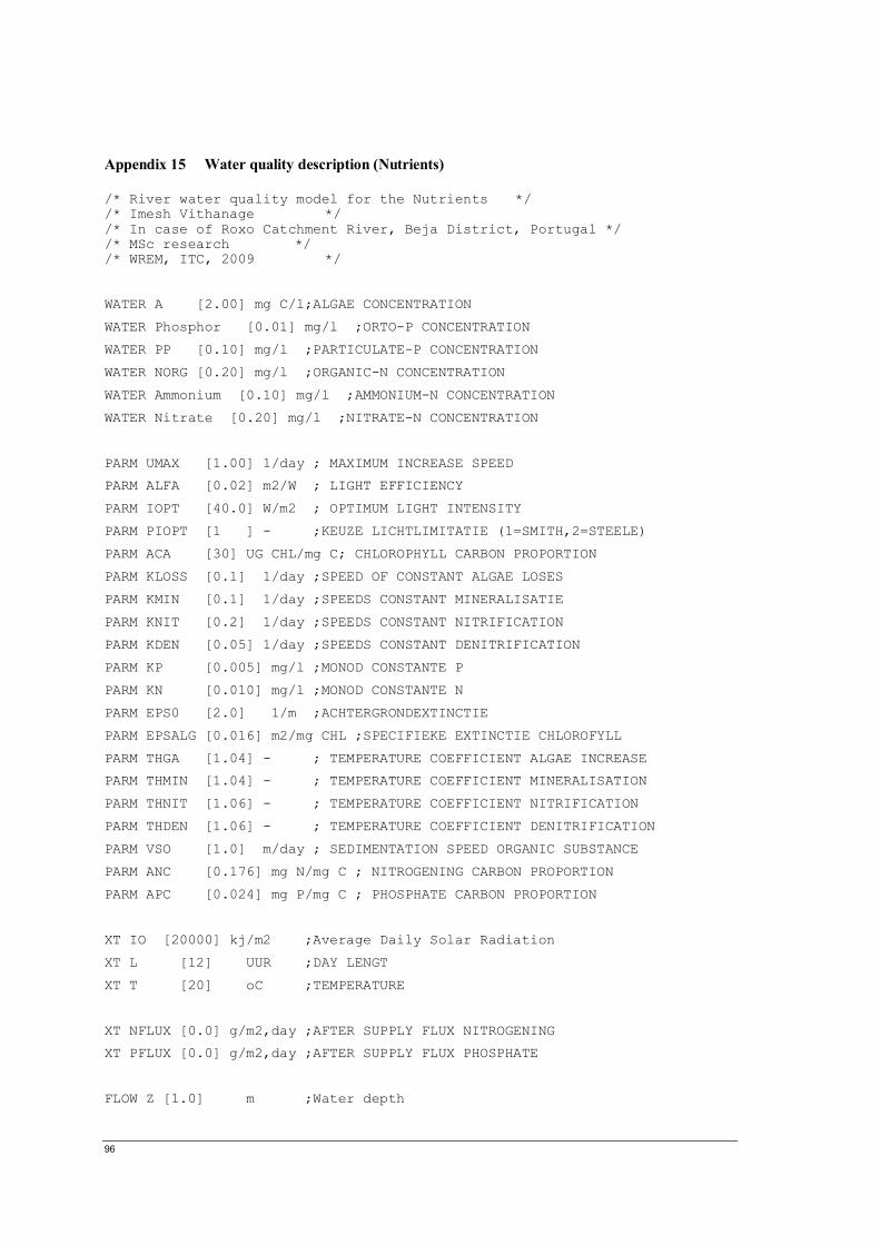
96
Appendix 15 Water quality description (Nutrients) /* River water quality model for the Nutrients */ /* Imesh Vithanage */ /* In case of Roxo Catchment River, Beja District, Portugal */ /* MSc research */ /* WREM, ITC, 2009 */ WATER A [2.00] mg C/l;ALGAE CONCENTRATION
WATER Phosphor [0.01] mg/l ;ORTO-P CONCENTRATION
WATER PP [0.10] mg/l ;PARTICULATE-P CONCENTRATION
WATER NORG [0.20] mg/l ;ORGANIC-N CONCENTRATION
WATER Ammonium [0.10] mg/l ;AMMONIUM-N CONCENTRATION
WATER Nitrate [0.20] mg/l ;NITRATE-N CONCENTRATION
PARM UMAX [1.00] 1/day ; MAXIMUM INCREASE SPEED
PARM ALFA [0.02] m2/W ; LIGHT EFFICIENCY
PARM IOPT [40.0] W/m2 ; OPTIMUM LIGHT INTENSITY
PARM PIOPT [1 ] - ;KEUZE LICHTLIMITATIE (1=SMITH,2=STEELE)
PARM ACA [30] UG CHL/mg C; CHLOROPHYLL CARBON PROPORTION
PARM KLOSS [0.1] 1/day ;SPEED OF CONSTANT ALGAE LOSES
PARM KMIN [0.1] 1/day ;SPEEDS CONSTANT MINERALISATIE
PARM KNIT [0.2] 1/day ;SPEEDS CONSTANT NITRIFICATION
PARM KDEN [0.05] 1/day ;SPEEDS CONSTANT DENITRIFICATION
PARM KP [0.005] mg/l ;MONOD CONSTANTE P
PARM KN [0.010] mg/l ;MONOD CONSTANTE N
PARM EPS0 [2.0] 1/m ;ACHTERGRONDEXTINCTIE
PARM EPSALG [0.016] m2/mg CHL ;SPECIFIEKE EXTINCTIE CHLOROFYLL
PARM THGA [1.04] - ; TEMPERATURE COEFFICIENT ALGAE INCREASE
PARM THMIN [1.04] - ; TEMPERATURE COEFFICIENT MINERALISATION
PARM THNIT [1.06] - ; TEMPERATURE COEFFICIENT NITRIFICATION
PARM THDEN [1.06] - ; TEMPERATURE COEFFICIENT DENITRIFICATION
PARM VSO [1.0] m/day ; SEDIMENTATION SPEED ORGANIC SUBSTANCE
PARM ANC [0.176] mg N/mg C ; NITROGENING CARBON PROPORTION
PARM APC [0.024] mg P/mg C ; PHOSPHATE CARBON PROPORTION
XT IO [20000] kj/m2 ;Average Daily Solar Radiation
XT L [12] UUR ;DAY LENGT
XT T [20] oC ;TEMPERATURE
XT NFLUX [0.0] g/m2,day ;AFTER SUPPLY FLUX NITROGENING
XT PFLUX [0.0] g/m2,day ;AFTER SUPPLY FLUX PHOSPHATE
FLOW Z [1.0] m ;Water depth

Analysis of Nutrient Dynamics in Roxo Catchment Using Remote Sensing data and Numerical Modeling
97
{
FT=THGA^(T-20);
FN=MIN(Phosphor/(Phosphor+KP),Ammonium/(Ammonium+KN));
IOMAX=1000*2*IO/(L*3600);
CHLA=ACA*A;
ETOT=EPS0+EPSALG*CHLA;
IF (PIOPT==1)
{
H1=(1+(ALFA*IOMAX)^2)^0.5;
FL=L*(LN(ALFA*IOMAX+H1+(1-H1)/(ALFA*IOMAX)))/(24*ETOT*Z);
}
IF (PIOPT==2)
{
f=(L/24);
ALFA1=ALFA*exp(-1*ETOT*Z);
FL=2.718*f*(exp(-1*ALFA1)-exp(-1*ALFA))/(ETOT*Z);
}
GA=UMAX*FT*FN*FL;
K1(A)=GA-KLOSS;
KMINT=KMIN*THMIN^(T-20);
K1(NORG)=-KMINT-VSO/Z;
K0(NORG)=KLOSS*ANC*A;
KNITT=KNIT*THNIT^(T-20);
K1(Ammonium)=-KNITT;
K0(Ammonium)=KMINT*NORG-GA*ANC*A+NFLUX/Z;
KDENT=KDEN*THDEN^(T-20);
K1(Nitrate)=-KDENT;
K0(Nitrate)=KNITT*Ammonium;
K1(PP)=-KMINT-VSO/Z;
K0(PP)=KLOSS*APC*A;
K1(Phosphor)=0;
K0(Phosphor)=KMINT*PP-GA*APC*A+PFLUX/Z;
KJN=NORG+Ammonium+ANC*A;
NTOT=KJN+Nitrate;
PTOT=PP+Phosphor+APC*A;
}
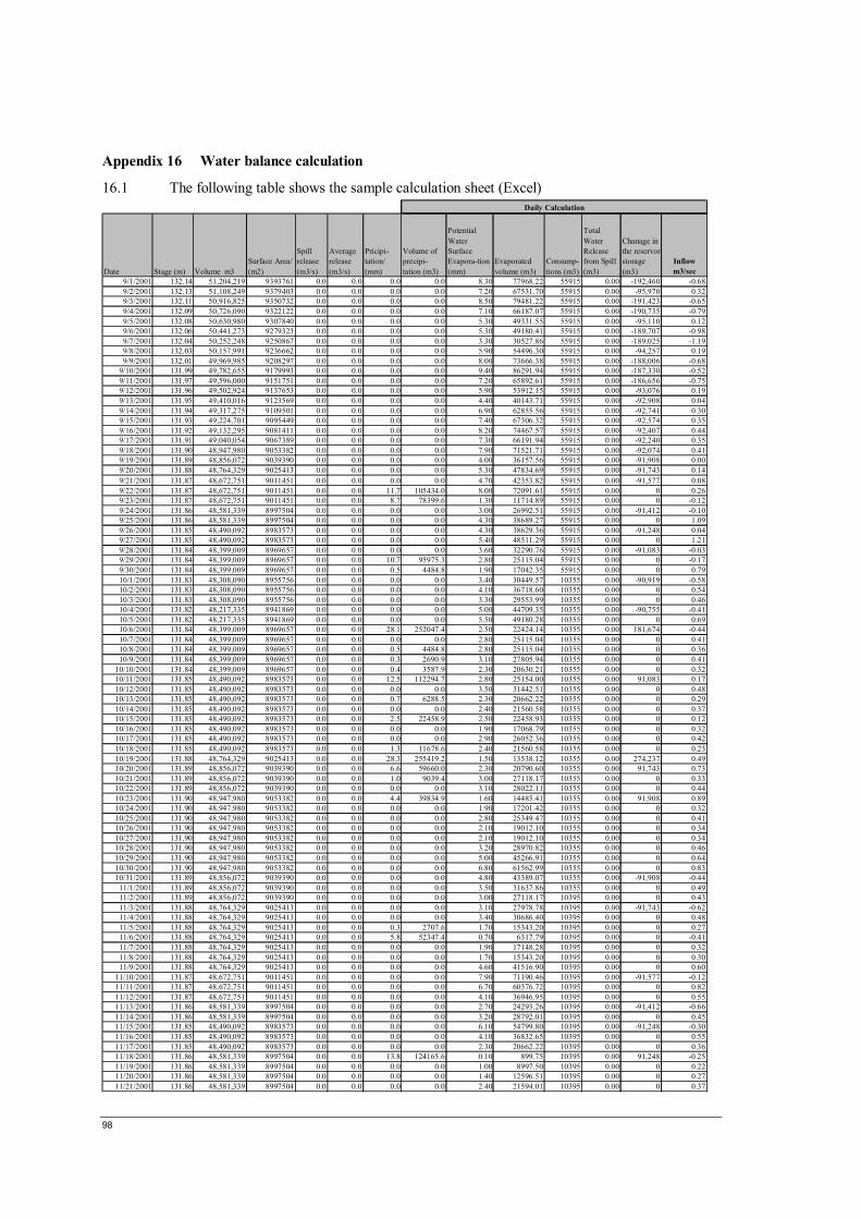
98
Appendix 16 Water balance calculation
16.1 The following table shows the sample calculation sheet (Excel)
Date Stage (m) Volume m3Surface Area/ (m2)
Spill release (m3/s)
Average release (m3/s)
Pricipi- tation/ (mm)
Volume of precipi-tation (m3)
Potential Water Surface Evapora-tion (mm)
Evaporated volume (m3)
Consump-tions (m3)
Total Water Release from Spill (m3)
Chanage in the reservor storage (m3)
Inflow m3/sec
9/1/2001 132.14 51,204,219 9393761 0.0 0.0 0.0 0.0 8.30 77968.22 55915 0.00 -192,460 -0.689/2/2001 132.13 51,108,249 9379403 0.0 0.0 0.0 0.0 7.20 67531.70 55915 0.00 -95,970 0.329/3/2001 132.11 50,916,825 9350732 0.0 0.0 0.0 0.0 8.50 79481.22 55915 0.00 -191,423 -0.659/4/2001 132.09 50,726,090 9322122 0.0 0.0 0.0 0.0 7.10 66187.07 55915 0.00 -190,735 -0.799/5/2001 132.08 50,630,980 9307840 0.0 0.0 0.0 0.0 5.30 49331.55 55915 0.00 -95,110 0.129/6/2001 132.06 50,441,273 9279323 0.0 0.0 0.0 0.0 5.30 49180.41 55915 0.00 -189,707 -0.989/7/2001 132.04 50,252,248 9250867 0.0 0.0 0.0 0.0 3.30 30527.86 55915 0.00 -189,025 -1.199/8/2001 132.03 50,157,991 9236662 0.0 0.0 0.0 0.0 5.90 54496.30 55915 0.00 -94,257 0.199/9/2001 132.01 49,969,985 9208297 0.0 0.0 0.0 0.0 8.00 73666.38 55915 0.00 -188,006 -0.68
9/10/2001 131.99 49,782,655 9179993 0.0 0.0 0.0 0.0 9.40 86291.94 55915 0.00 -187,330 -0.529/11/2001 131.97 49,596,000 9151751 0.0 0.0 0.0 0.0 7.20 65892.61 55915 0.00 -186,656 -0.759/12/2001 131.96 49,502,924 9137653 0.0 0.0 0.0 0.0 5.90 53912.15 55915 0.00 -93,076 0.199/13/2001 131.95 49,410,016 9123569 0.0 0.0 0.0 0.0 4.40 40143.71 55915 0.00 -92,908 0.049/14/2001 131.94 49,317,275 9109501 0.0 0.0 0.0 0.0 6.90 62855.56 55915 0.00 -92,741 0.309/15/2001 131.93 49,224,701 9095449 0.0 0.0 0.0 0.0 7.40 67306.32 55915 0.00 -92,574 0.359/16/2001 131.92 49,132,295 9081411 0.0 0.0 0.0 0.0 8.20 74467.57 55915 0.00 -92,407 0.449/17/2001 131.91 49,040,054 9067389 0.0 0.0 0.0 0.0 7.30 66191.94 55915 0.00 -92,240 0.359/18/2001 131.90 48,947,980 9053382 0.0 0.0 0.0 0.0 7.90 71521.71 55915 0.00 -92,074 0.419/19/2001 131.89 48,856,072 9039390 0.0 0.0 0.0 0.0 4.00 36157.56 55915 0.00 -91,908 0.009/20/2001 131.88 48,764,329 9025413 0.0 0.0 0.0 0.0 5.30 47834.69 55915 0.00 -91,743 0.149/21/2001 131.87 48,672,751 9011451 0.0 0.0 0.0 0.0 4.70 42353.82 55915 0.00 -91,577 0.089/22/2001 131.87 48,672,751 9011451 0.0 0.0 11.7 105434.0 8.00 72091.61 55915 0.00 0 0.269/23/2001 131.87 48,672,751 9011451 0.0 0.0 8.7 78399.6 1.30 11714.89 55915 0.00 0 -0.129/24/2001 131.86 48,581,339 8997504 0.0 0.0 0.0 0.0 3.00 26992.51 55915 0.00 -91,412 -0.109/25/2001 131.86 48,581,339 8997504 0.0 0.0 0.0 0.0 4.30 38689.27 55915 0.00 0 1.099/26/2001 131.85 48,490,092 8983573 0.0 0.0 0.0 0.0 4.30 38629.36 55915 0.00 -91,248 0.049/27/2001 131.85 48,490,092 8983573 0.0 0.0 0.0 0.0 5.40 48511.29 55915 0.00 0 1.219/28/2001 131.84 48,399,009 8969657 0.0 0.0 0.0 0.0 3.60 32290.76 55915 0.00 -91,083 -0.039/29/2001 131.84 48,399,009 8969657 0.0 0.0 10.7 95975.3 2.80 25115.04 55915 0.00 0 -0.179/30/2001 131.84 48,399,009 8969657 0.0 0.0 0.5 4484.8 1.90 17042.35 55915 0.00 0 0.7910/1/2001 131.83 48,308,090 8955756 0.0 0.0 0.0 0.0 3.40 30449.57 10355 0.00 -90,919 -0.5810/2/2001 131.83 48,308,090 8955756 0.0 0.0 0.0 0.0 4.10 36718.60 10355 0.00 0 0.5410/3/2001 131.83 48,308,090 8955756 0.0 0.0 0.0 0.0 3.30 29553.99 10355 0.00 0 0.4610/4/2001 131.82 48,217,335 8941869 0.0 0.0 0.0 0.0 5.00 44709.35 10355 0.00 -90,755 -0.4110/5/2001 131.82 48,217,335 8941869 0.0 0.0 0.0 0.0 5.50 49180.28 10355 0.00 0 0.6910/6/2001 131.84 48,399,009 8969657 0.0 0.0 28.1 252047.4 2.50 22424.14 10355 0.00 181,674 -0.4410/7/2001 131.84 48,399,009 8969657 0.0 0.0 0.0 0.0 2.80 25115.04 10355 0.00 0 0.4110/8/2001 131.84 48,399,009 8969657 0.0 0.0 0.5 4484.8 2.80 25115.04 10355 0.00 0 0.3610/9/2001 131.84 48,399,009 8969657 0.0 0.0 0.3 2690.9 3.10 27805.94 10355 0.00 0 0.41
10/10/2001 131.84 48,399,009 8969657 0.0 0.0 0.4 3587.9 2.30 20630.21 10355 0.00 0 0.3210/11/2001 131.85 48,490,092 8983573 0.0 0.0 12.5 112294.7 2.80 25154.00 10355 0.00 91,083 0.1710/12/2001 131.85 48,490,092 8983573 0.0 0.0 0.0 0.0 3.50 31442.51 10355 0.00 0 0.4810/13/2001 131.85 48,490,092 8983573 0.0 0.0 0.7 6288.5 2.30 20662.22 10355 0.00 0 0.2910/14/2001 131.85 48,490,092 8983573 0.0 0.0 0.0 0.0 2.40 21560.58 10355 0.00 0 0.3710/15/2001 131.85 48,490,092 8983573 0.0 0.0 2.5 22458.9 2.50 22458.93 10355 0.00 0 0.1210/16/2001 131.85 48,490,092 8983573 0.0 0.0 0.0 0.0 1.90 17068.79 10355 0.00 0 0.3210/17/2001 131.85 48,490,092 8983573 0.0 0.0 0.0 0.0 2.90 26052.36 10355 0.00 0 0.4210/18/2001 131.85 48,490,092 8983573 0.0 0.0 1.3 11678.6 2.40 21560.58 10355 0.00 0 0.2310/19/2001 131.88 48,764,329 9025413 0.0 0.0 28.3 255419.2 1.50 13538.12 10355 0.00 274,237 0.4910/20/2001 131.89 48,856,072 9039390 0.0 0.0 6.6 59660.0 2.30 20790.60 10355 0.00 91,743 0.7310/21/2001 131.89 48,856,072 9039390 0.0 0.0 1.0 9039.4 3.00 27118.17 10355 0.00 0 0.3310/22/2001 131.89 48,856,072 9039390 0.0 0.0 0.0 0.0 3.10 28022.11 10355 0.00 0 0.4410/23/2001 131.90 48,947,980 9053382 0.0 0.0 4.4 39834.9 1.60 14485.41 10355 0.00 91,908 0.8910/24/2001 131.90 48,947,980 9053382 0.0 0.0 0.0 0.0 1.90 17201.42 10355 0.00 0 0.3210/25/2001 131.90 48,947,980 9053382 0.0 0.0 0.0 0.0 2.80 25349.47 10355 0.00 0 0.4110/26/2001 131.90 48,947,980 9053382 0.0 0.0 0.0 0.0 2.10 19012.10 10355 0.00 0 0.3410/27/2001 131.90 48,947,980 9053382 0.0 0.0 0.0 0.0 2.10 19012.10 10355 0.00 0 0.3410/28/2001 131.90 48,947,980 9053382 0.0 0.0 0.0 0.0 3.20 28970.82 10355 0.00 0 0.4610/29/2001 131.90 48,947,980 9053382 0.0 0.0 0.0 0.0 5.00 45266.91 10355 0.00 0 0.6410/30/2001 131.90 48,947,980 9053382 0.0 0.0 0.0 0.0 6.80 61562.99 10355 0.00 0 0.8310/31/2001 131.89 48,856,072 9039390 0.0 0.0 0.0 0.0 4.80 43389.07 10355 0.00 -91,908 -0.44
11/1/2001 131.89 48,856,072 9039390 0.0 0.0 0.0 0.0 3.50 31637.86 10355 0.00 0 0.4911/2/2001 131.89 48,856,072 9039390 0.0 0.0 0.0 0.0 3.00 27118.17 10395 0.00 0 0.4311/3/2001 131.88 48,764,329 9025413 0.0 0.0 0.0 0.0 3.10 27978.78 10395 0.00 -91,743 -0.6211/4/2001 131.88 48,764,329 9025413 0.0 0.0 0.0 0.0 3.40 30686.40 10395 0.00 0 0.4811/5/2001 131.88 48,764,329 9025413 0.0 0.0 0.3 2707.6 1.70 15343.20 10395 0.00 0 0.2711/6/2001 131.88 48,764,329 9025413 0.0 0.0 5.8 52347.4 0.70 6317.79 10395 0.00 0 -0.4111/7/2001 131.88 48,764,329 9025413 0.0 0.0 0.0 0.0 1.90 17148.28 10395 0.00 0 0.3211/8/2001 131.88 48,764,329 9025413 0.0 0.0 0.0 0.0 1.70 15343.20 10395 0.00 0 0.3011/9/2001 131.88 48,764,329 9025413 0.0 0.0 0.0 0.0 4.60 41516.90 10395 0.00 0 0.60
11/10/2001 131.87 48,672,751 9011451 0.0 0.0 0.0 0.0 7.90 71190.46 10395 0.00 -91,577 -0.1211/11/2001 131.87 48,672,751 9011451 0.0 0.0 0.0 0.0 6.70 60376.72 10395 0.00 0 0.8211/12/2001 131.87 48,672,751 9011451 0.0 0.0 0.0 0.0 4.10 36946.95 10395 0.00 0 0.5511/13/2001 131.86 48,581,339 8997504 0.0 0.0 0.0 0.0 2.70 24293.26 10395 0.00 -91,412 -0.6611/14/2001 131.86 48,581,339 8997504 0.0 0.0 0.0 0.0 3.20 28792.01 10395 0.00 0 0.4511/15/2001 131.85 48,490,092 8983573 0.0 0.0 0.0 0.0 6.10 54799.80 10395 0.00 -91,248 -0.3011/16/2001 131.85 48,490,092 8983573 0.0 0.0 0.0 0.0 4.10 36832.65 10395 0.00 0 0.5511/17/2001 131.85 48,490,092 8983573 0.0 0.0 0.0 0.0 2.30 20662.22 10395 0.00 0 0.3611/18/2001 131.86 48,581,339 8997504 0.0 0.0 13.8 124165.6 0.10 899.75 10395 0.00 91,248 -0.2511/19/2001 131.86 48,581,339 8997504 0.0 0.0 0.0 0.0 1.00 8997.50 10395 0.00 0 0.2211/20/2001 131.86 48,581,339 8997504 0.0 0.0 0.0 0.0 1.40 12596.51 10395 0.00 0 0.2711/21/2001 131.86 48,581,339 8997504 0.0 0.0 0.0 0.0 2.40 21594.01 10395 0.00 0 0.37
Daily Calculation
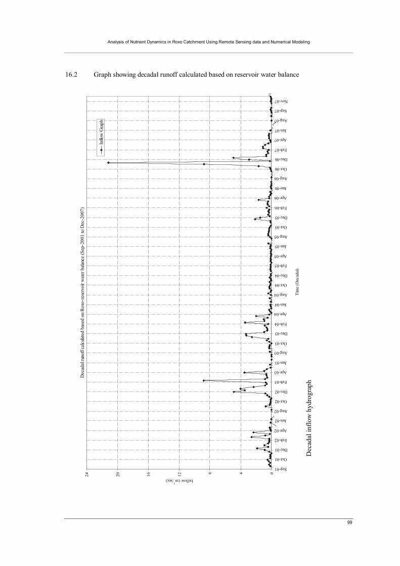
Analysis of Nutrient Dynamics in Roxo Catchment Using Remote Sensing data and Numerical Modeling
99
16.2 Graph showing decadal runoff calculated based on reservoir water balance
Dec
adal
inflo
w h
ydro
grap
h
Dec
adal
runo
ff ca
lculat
ed b
ased
on
Roxo
-res
ervo
ir w
ater
bala
nce
(Sep
-200
1 to
Dec
-200
7)
04812162024
Sep-01
Oct-01
Dec-01
Feb-02
Apr-02
Jun-02
Aug-02
Oct-02
Dec-02
Feb-03
Apr-03
Jun-03
Aug-03
Oct-03
Dec-03
Feb-04
Apr-04
Jun-04
Aug-04
Oct-04
Dec-04
Feb-05
Apr-05
Jun-05
Aug-05
Oct-05
Dec-05
Feb-06
Apr-06
Jun-06
Aug-06
Oct-06
Dec-06
Feb-07
Apr-07
Jun-07
Aug-07
Sep-07
Nov-07
Tim
e (D
ecad
al)
Inflow (m3/sec)
Inflo
w G
raph

100
Appendix 17 Results of the sensitivity analysis
Root mean squared error
Relative volume error
Nash Shutcliffe
k=0.0014 1.288 44.0% -0.11k= 0.00 1.288 44.0% -0.11k =0.0014 1.288 44.0% -0.11k =0.01 1.288 44.0% -0.11k =1 1.288 43.8% -0.11
Imax=25 1.288 43.8% -0.11
Imax =10 1.288 43.8% -0.11DH=0.2 3.143 150.2% -5.59DH=0.3 3.815 229.9% -8.71DH=0.15 2.306 108.4% -2.55DH=0.12 1.777 71.6% -1.11
DH=0.08 1.130 17.7% 0.15
DH=0.05 1.124 -15.1% 0.16DH=0.07 1.104 3.3% 0.19DH=0.09 1.153 30.6% 0.11DH=0.075 1.101 9.8% 0.19C=250 1.099 5.7% 0.19C=275 1.114 -0.1% 0.17C=200 1.153 30.6% 0.11C=175 1.347 50.3% -0.21C=235 1.097 12.1% 0.20C=215 1.150 23.7% 0.12C=260 1.103 3.4% 0.19C=300 1.133 -4.9% 0.14C=175 3.553 194.5% -7.42C=300 2.306 108.4% -2.55C=350 1.900 78.5% -1.41C=400 1.577 63.9% -0.66C=500 1.161 30.9% 0.10C=550 1.115 18.6% 0.17C=530 1.145 26.3% 0.13C=510 1.179 28.5% 0.07C=520 1.162 25.8% 0.10C=525 1.158 26.2% 0.11Imax=25 2.666 332.8% -3.74Imax=30 1.158 -40.0% 0.11Imax=28 1.173 -39.1% 0.08Imax=32 1.147 -40.7% 0.12Imax=40 1.146 -41.0% 0.12Imax=20 1.360 -28.2% -0.23LBvo = 1000 1.129 -37.3% 0.15LBvo = 1500 1.244 -62.3% -0.03LBvo = 1200 1.196 -50.6% 0.05LBvo = 1000 2.736 111.6% -3.99LBvo = 1100 2.472 99.1% -3.08LBvo = 1100 1.190 30.0% 0.06
Unpaved Surface
C (days) DH=0.08 m
C (days) DH=0.2 m
k (day)
Imax (mm/day)
Lbvo (mm)
k (day)Open water
Paved Surface
Seepage
Imax (mm/day)
DH (m) C=225 days
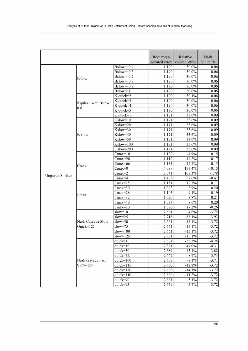
Analysis of Nutrient Dynamics in Roxo Catchment Using Remote Sensing data and Numerical Modeling
101
Root mean squared error
Relative volume error
Nash Shutcliffe
Bslow = 0.4 1.190 30.0% 0.06Bslow = 0.3 1.190 30.0% 0.06Bslow = 0.7 1.190 30.0% 0.06Bslow = 0.8 1.190 30.0% 0.06Bslow = 0.9 1.190 30.0% 0.06Bslow = 1 1.190 30.0% 0.06K quick=2 1.190 30.1% 0.06K quick=3 1.190 30.0% 0.06K quick=4 1.190 30.0% 0.06K quick=5 1.190 30.0% 0.06K quick=1 1.171 33.6% 0.09Kslow=10 1.171 33.6% 0.09Kslow=20 1.171 33.6% 0.09Kslow=30 1.171 33.6% 0.09Kslow=40 1.171 33.6% 0.09Kslow=50 1.171 33.6% 0.09Kslow=100 1.171 33.6% 0.09Kslow=200 1.171 33.6% 0.09Cmax=10 1.130 -4.9% 0.15Cmax=20 1.112 -14.2% 0.17Cmax=66 1.131 -12.7% 0.15Cmax=0 4.089 197.4% -10.15Cmax=2 2.041 108.3% -1.78Cmax=4 1.486 57.6% -0.47I max=25 1.154 12.3% 0.11I max=30 1.093 8.9% 0.20I max=28 1.103 9.1% 0.19I max=32 1.090 8.8% 0.21I max=40 1.094 8.6% 0.20I max=20 1.376 17.2% -0.26slow=10 2.661 4.6% -3.72slow=25 2.718 -86.1% -3.93slow=50 2.661 -15.1% -3.72slow=75 2.661 -15.1% -3.72slow=100 2.661 -15.1% -3.72slow=125 2.661 -15.1% -3.72quick=1 2.804 -38.3% -4.25quick=10 2.821 47.0% -4.31quick=50 2.689 45.1% -3.82quick=75, 2.662 8.7% -3.73quick=100 2.658 -8.1% -3.71quick=115 2.660 -12.8% -3.72quick=120 2.660 -14.1% -3.72quick=110 2.660 -11.2% -3.72quick=90 2.661 -3.1% -3.72quick=95 2.659 -5.7% -3.72
Unpaved Surface
Nash Cascade Slow Quick=125
Nash cascade Fast Slow=125
I max
Bslow
Kquick with Bslow 0.6
K slow
Cmax
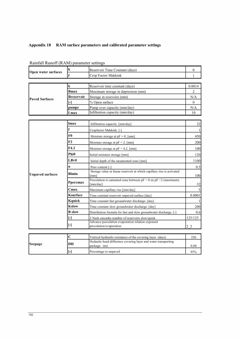
102
Appendix 18 RAM surface parameters and calibrated parameter settings
k Reservoir Time Constant (days) 0f Crop Factor Makkink 1
k Reservoir time constant (days) 0.0014Bmax Maximum storage in depression (mm) 2Breservoir Storage in resevoirs (mm) N/A[-] % Open surface 0pumpc Pump over capacity (mm/day) N/AI max Infiltration capacity (mm/day) 10
Imax Infiltration capacity. [mm/day] 32f Cropfactor Makkink. [-] 1F0 Moisture storage at pF = 0. [mm] 450F2 Moisture storage at pF = 2. [mm] 200F4.2 Moisture storage at pF = 4.2. [mm] 100Phi0 Initial moisture storage [mm] 120LBv0 Initial depth of the unsaturated zone [mm] 1100n Pore content [-] 0.5
Blmin Storage value in linear reservoir at which capillary rise is activated [mm] 100
Ppercmax Percolation to saturated zone between pF = 0 en pF =2 (maximum). [mm/day] 32
Cmax Maximum capillary rise [mm/day] 5Ksurface Time constant reservoir unpaved surface [day] 0.0001Kquick Time constant fast groundwater discharge. [day] 1Kslow Time constant slow groundwater discharge. [day] 200B slow Distribution formula for fast and slow groundwater discharge. [-] 0.6[-] 2 Nash cascades number of reservoirs slow/quick 125/125
[-]Advance percolation evaporation relation exponent percolation/evaporation 2_2
C Vertical hydraulic resistance of the covering layer (days) 250
DH Hydaulic head difference covering layer and water transporting package (m) 0.08
[-] Percentage to unpaved 95%
Rainfall Runoff (RAM) parameter settings
Open water surfaces
Paved Surfaces
Unpaved surfaces
Seepage

Analysis of Nutrient Dynamics in Roxo Catchment Using Remote Sensing data and Numerical Modeling
103
Appendix 19 Temporal Phosphates concentration and load variation at reservoir section (SEC00028:NOD00025->CLC00211)
Temporal Phophate Concentration variation at reservoir section SEC00028:NOD00025->CLC00211
0
0.2
0.4
0.6
0.8
1
1.2
1.4
1.6
1.8
2
Sep-
01
Nov
-01
Feb-
02
May
-02
Aug
-02
Nov
-02
Feb-
03
May
-03
Aug
-03
Nov
-03
Feb-
04
May
-04
Aug
-04
Nov
-04
Feb-
05
May
-05
Aug
-05
Nov
-05
Feb-
06
May
-06
Aug
-06
Nov
-06
Feb-
07
May
-07
Aug
-07
Oct
-07
Time
Phos
phat
e co
ncen
tratio
n (m
g/l)
llll
Phophate Concentration
fig.(a) Phosphor - Concentration
Temporal Phophate load variation at reservoir section SEC00028:NOD00025->CLC00211
0
1
2
3
4
5
6
Sep-
01
Nov
-01
Feb-
02
May
-02
Aug
-02
Nov
-02
Feb-
03
May
-03
Aug
-03
Nov
-03
Feb-
04
May
-04
Aug
-04
Nov
-04
Feb-
05
May
-05
Aug
-05
Nov
-05
Feb-
06
May
-06
Aug
-06
Nov
-06
Feb-
07
May
-07
Aug
-07
Oct
-07
Time
Phos
phat
e Lo
ad (g
/s) l
lll
Phophate Load g/s
fig.(b) Phosphor -Loads