Analysis of Households’ Decision Using Full Demand

HAL Id: halshs-01491970https://halshs.archives-ouvertes.fr/halshs-01491970

Submitted on 17 Mar 2017

HAL is a multi-disciplinary open accessarchive for the deposit and dissemination of sci-entific research documents, whether they are pub-lished or not. The documents may come fromteaching and research institutions in France orabroad, or from public or private research centers.

L’archive ouverte pluridisciplinaire HAL, estdestinée au dépôt et à la diffusion de documentsscientifiques de niveau recherche, publiés ou non,émanant des établissements d’enseignement et derecherche français ou étrangers, des laboratoirespublics ou privés.

Analysis of Households’ Decision Using Full DemandElasticity Estimates: an Estimation on Turkish Data

Okay Gunes

To cite this version:Okay Gunes. Analysis of Households’ Decision Using Full Demand Elasticity Estimates: an Estimationon Turkish Data. 2017. �halshs-01491970�

https://halshs.archives-ouvertes.fr/halshs-01491970

https://hal.archives-ouvertes.fr

Documents de Travail du Centre d’Economie de la Sorbonne

Analysis of Households’ Decision Using Full Demand

Elasticity Estimates: an Estimation on Turkish Data

Okay GUNES

2017.17

Maison des Sciences Économiques, 106-112 boulevard de L'Hôpital, 75647 Paris Cedex 13 http://centredeconomiesorbonne.univ-paris1.fr/

ISSN : 1955-611X

1

Analysis of Households' Decision Using Full Demand Elasticity Estimates: an Estimation on Turkish Data

Okay Gunes*

Abstract

Households’ consumption patterns are deciphered through estimates of demand elasticities based on the domestic production decisions determined by constraints on time use and monetary budgets for different subpopulations. We first estimate the shadow wage rates of the households and later estimate the full demand elasticities which are computed using full prices proposed by Gardes (2016) derived through the hypotheses of complementarity or substitutability existing between monetary and time expenditures. Detailed results are obtained for the whole population by breaking the dataset into age groups and into households according to poverty level, as determined by the OECD-modified equivalence scale.

JEL: C1, D1, D13, J22 Keywords: Time allocation, domestic production, full prices, opportunity cost of time, demand elasticities, Rubins’ matching statistics. I. Introduction

Studies of demand patterns have become an increasingly important feature in political interventions regarding the problem of income distribution and of welfare analysis. Analysis of consumer behavior provides an important insight into how economic agents react to changes in prices, income and furthermore, in individual time use. In fact, there have been some promising works on developments in integrating time allocation decisions into consumer choice, as the extension of the traditional theory becomes more challenging particularly in the wake of works by Mincer (1963) and Becker (1965). Their works opened up new problematic areas regarding the role of time use in consumer decisions and are still yet to be fully verified by demand system analysis.

Time allocation models provide useful information concerning measurement of the price of time as shadow wages since the difficulties encountered in exchanging time between two individuals imply that no market price exists for time. One common method in the theoretical applications of microeconomic models is to introduce a time equation as a supplementary constraint in consumer optimisation in order to measure the monetary value of time1. Essentially, microeconomic time allocation models determine the opportunity cost of time that results from specific time and budget constraints in concert, giving the ratio of Lagrange multipliers as the monetary value of time. That is to say: consumers maximize their direct utility function depending on the time spent and on commodities, if it is supposed that the commodities are Hicksian composite goods and the relative prices of all market goods are

* Université Paris I Panthéon-Sorbonne, Centre d’Economie de la Sorbonne, 106-112 Boulevard de l’Hôpital, 75647, Paris Cedex 13, France; tel : 01 44 07 82 87 ; e-mail: [email protected] 1 Becker (1965) supposed that the household can imply trade-off time for money, and so only faces the single budget constraint. However, value of time would also result from the time partition defined within the time constraint equation. See Johnson, 1966; Oort, 1969; DeSerpa, 1971; Evans, 1972; Small, 1982; Gronau, 1986; Jara-Diaz et al., 2013).

Documents de travail du Centre d'Economie de la Sorbonne - 2017.17

2

constant across the population. It is then further supposed that there is a perfect substitution between market and domestic labor2.

Another method to measure the value of time use is to suppose that the opportunity cost of domestic activities is considered as the average net wage rate for all working individuals in the family, or as their expected hourly wage rate in the labor market for non-working individuals. In general, the two-step Heckman estimation procedure enables researchers to predict opportunity cost of non-working individuals. This method is based on a hypothesis of an existing perfectly exchangeable structure between market and non market household activities.

Another possibility for determining opportunity cost is using the hourly minimum wage in the market in order to evaluate time spent in domestic activities. However, the vast majority of household demand models today make the fixed wage assumption. As a matter of fact, difficulties determining a convenient opportunity cost would be expected to bias the measurement of time allocation decisions, especially for those in developing economies for two reasons: firstly, if consumers all pay the same market prices for consumption goods, variation in earnings across individuals results in cross-sectional variation in the shadow prices for consumption goods and, as a result, estimated Engel curves will, by omitting these shadow price effects, tend to underestimate the true income effects of earnings intensive goods3. Secondly, it is more convenient to assume that monetary expenditures are determined by domestic production technology and by time scarcity which in turn determines the shadow wage rates. If labor supply is supposed to be endogenously determined under market conditions, time scarcity (i.e. used for the domestic production) depends totally on the relationship between income and non-labor time. The higher the labor supply and the lower the non-labor time, hence the greater the shadow price of time4 and good intensive consumption. However, it is still optimistic to believe that in the case of developing economies, that average time costs are equal to marginal time costs of different activities and that marginal costs are what determine behavior. In fact, constraints in elastic labor markets may increase the adjustment and transaction costs which would in turn likely render shadow wages lower than market wage rates. Thus, it becomes more reasonable to consider that shadow wages are expected to be different among activities and that households may try to compensate any loss due to market constraints or to inflation and decreasing incomes by replacing monetary expenditures with domestic production, which in turn depends on the capacity of combining time spent with market commodities. Be that as it may, for any given shadow wage rate, the welfare of households would depend on the complementary and substitutable nature of household domestic production5.

There are relatively few studies in which time allocation theory is systematically applied to the practical estimation of the demand elasticities6. Our aim in this paper is to estimate the

2 Thus, marginal rate of substitution between the marginal utilities of time use and market expenditure determines the shadow price as the wage rate divided by the price of market good. 3 See Chiappori and Lewbel (2015) 4 See Gronau (1986). 5 Time spent and commodity use can be both substitutable and complementary at a certain level depending on the type of the activity and on socioeconomic characteristics of households. For the discussion see Gronau and Hamermesh, 2006; Hamermesh, 2008; Baral et al., 2011; and Davis and You, 2013. 6 Aktuna Gunes et al (2016), for the working papers see Aktuna Gunes et al(2013) and Canelas et al. (2013).


3

values of income and price elasticities by integrating the time use values into a complete demand system, taking into consideration the existing complementarity and substitution between inputs used in domestic production for Turkey. To this end, we determine representative shadow wage rates by measuring opportunity cost of time values with respect to activity group for subpopulations defined by age groups, income per unit of consumption, location and family structure. Later, demand elasticities are analyzed for the whole population and by breaking down the dataset into age groups and according to poverty level, as determined by the OECD-modified equivalence scale for Turkey.

Section 2 presents the construction of individual prices from a micro dataset using time values and presents the theoretical specification to estimate shadow wages based on a complete model proposed by Gardes (2016). Section 3 describes our sample and provides descriptive statistics for Turkey from the Household Budget Surveys 2007 and Time Use Surveys for 2006. Section 4 reports the results. Section 5 offers concluding remarks.

II. Demand System Specification to Estimate Full Price Elasticities

It is commonly thought that using macro time-series is a generally less robust method for estimating demand elasticities, since they give no information on how changes in price and income affect the household characteristics, or if existing co-linearity between relative prices changes, how aggregation biases are affected whenever individual agents face different prices changes or have different preferences. Gardes (2016) proposed a model which provides estimates for different commodity groups in absence of real price data, which can contribute to solving the problem of there being a lack of reliable sources of local price data in most developing countries. Moreover, this model framework allows us to measure the monetary value of domestic production. Full Prices

Following the time allocation theory by Becker (1965), full expenditure can simply be identified as7:

fi i i i ip z p x tω= + (1)

Where ω is the opportunity cost of time use activities, pf is the full price8 as the price index of final commodities (zi) and p denotes monetary prices. The equation measures the monetary

value of domestic production (��

��) by adding the monetary costs (pi xi) and monetary values

of time spent (ωti) for the activity i.

1. Full prices under Substitutable Factors: The full price is the derivative of the full expenditure given in equation (1) over zi , written as:

sf i ii i

i i

x tp p

z zω∂ ∂= +

∂ ∂ (2)

The index s in sfip is used to specify full price in terms of monetary value of marginal

substitution between time use and commodity use when domestic production is changing

7 Full derivation of the equations from (1) to (8) is given in the Appendix. 8 In fact, the price of final good Zi depends on the price of its input components. In the Beckerian theory, each final good is supposed to be homogeneous to degree 1. An invariant scale price index for each commodity can be constructed.


4

( iz∂ ). There are two information that can be gleaned from equation (2): The left hand side of

this equation is considered as full price since it is defined as a function of time use activities ti. Besides this it enables us derive how the price of domestic production changes.

2. Full prices proxies for complementary factors: Beckerian full price can directly be

written under the supposition that households require time to produce one unit of final goods as.

cfi i ip p ωτ= + (3)

Where index c denotes complementary specification of full price. Supposing that a Leontief technology allows the quantities of time and commodity factors to be proportional to the activity:

;i i i i i ix z t zξ θ= = (4)

which yields

i ii

i i

t

x

θτξ

= = (5)

Where iτ for the activity i represents the time unit per commodity as the scalar ratio

determined by the constant technology of combining goods and time to produce final goods. This case corresponds to an assumption of complementarity between these two factors in the domestic technology.

We can calculate a proxy for the full price of activity i by the ratio of full expenditure over

its monetary component. To show this, let iπ be the proxy of full price as the price ratio

given by /cfi ip p . The proxy of full price is simply the price ratio which can be obtained by

multiplying denominator and nominator with consumption amount xi. This is also the empirical definition of the full price as the ratio of full expenditures over their monetary component for activity i for the household h, which can be isolated as

cfih

ii

ihh

ih

ih

i

ihhiih p

ppx

x

p

p 11

)( =+=+= τωτωπ (6)

The denominator and the nominator in equation (6) respectively, are monetary expenditures and the full expenditure9 (i.e. monetary expenditures plus monetary time values used in domestic production). Thus, as can be seen from the right of the equation, the full prices no longer depend on consumption quantities.

Both definitions of full prices, sfip and cf

ip , are related to one another. To show this, using

the definition ;i i i i i i iim t m t t mα ω β ω ω= + = + we can derive

i

s i

β

f α ih h ihih i

i h ih i

m ω t1p = p 1+

a ω t p

(7)

9 This equation helps us to measure the full cost of consumptions which in turn allows us to obtain more adequate price elasticities. Itwas recently used to identify the reason underpinning informal activity participation, especially for emerging economies. See Armagan Tuna Aktuna-Gunes et al. (2016).


5

Where mi be monetary expenditure (pi xi).

Shadow Wages The opportunity cost of time (as the shadow wage rate) can be measured by

d

dd

T

m

m

u

T

t

t

u

Y

uT

u

∂∂

∂∂

∂∂

∂∂

=

∂∂∂∂

= '

'

'

'

ω (8)

Where di

iw TttT ==− ∑ with u, T, tw are the utility, total time and working time

respectively.

Estimating Full Price Elasticities According to this work, the Almost Ideal Demand System (AIDS) sample regression

function is estimated after the re-parameterization of the price parameters under the homogeneity, symmetry and additivity constraints for each consumption group, including full prices.

( ) ∑=

++++=n

jii

fjijiiih Zppxcsts cs

1

,loglog ελγδ (9)

s, x, p, ,s cfp and Z in (9) represent budget share, household expenditure, re-parameterized

Stone’s price index, full prices respectively for substitutable ( ��) and complementary ( ��) factors for each commodity group and socio-economic characteristics respectively for i th of n commodity group. The equation (9) is estimated separately for full prices respectively for substitutable ( ��) and complementary ( ��) factors. Let m be the translog price index defined by10:

jj k

kkjkk

k pppp lnln2

1lnlog 0 ∑∑∑ ++= γαα (10)

Demand-Elasticity

(i) Income Elasticity

Following the Green and Alston (1990) and Buse (1994) income elasticity and taking the derivation of equation (9) with respect to ln(x)¸ income elasticity Ex/y can be obtained as follows:

+=

∂∂

+=

i

i

i

i

iyx sx

s

sE

i

δ1

)ln(1

1/ (11)

10 Deaton and Muellbauer (1980), equation (9), p :314.


6

(ii) Price Elasticity

Following Green and Alston (1990), we derive price coefficients and demand system parameters for compensated price elasticities using AIDS, as follows:

−+−−+= ∑=

n

kj

fkkjj

i

iijj

i

ij

pxspcst

ss

sE cs

csfji

1/

,

, logˆ

γδξγ

(12)

Where ijξ is the Kronecker index with value 0=ijξ , if i j≠ and 1=ijξ , if i j= . In

equation (12) expressions the bars over variables represent averages. Following the method proposed by De Vany (1974), full price elasticities for each factor (�� and ��) would be directly calculated by summing up the Hicksian monetary and time elasticities respective to their shares.

, / //f

ijs

ic j i jx p x tx p

E E E= + (13)

In which the monetary price and time elasticities for each factor correspond respectively to

, , ,/ /i j i j

f fs c s c s c

j j

x xi jfp p

p

p

xE E

x= (14-i)

, ,/ /i j

i jfs c s c

j jx t fpx

i j

t xE

pE

x

ω= (14-ii)

III. Dataset and Matching Statistics

We use two household surveys: the Time use survey (TUS) in 2006 and the Household budget surveys (HBS) for the year 2007 from the Turkish Statistical Institute (TURKSTAT). The HBS has been conducted on a total of monthly 720 and annually 8640 households for 2007. Three basic groups of variables have been obtained from the survey: Variables of the socio-economic status of the households such as the status of property of house, living in village or in rural areas, etc; variables related to individuals (age, gender, academic background). Consumption expenditures variables (food and non alcoholic beverages, alcoholic beverages with cigarette and tobacco, clothing, health, transportation, education services, etc.) In the TUS in 2006, approximately 390 households were selected each month giving a total of 5070 households during the whole year. Within these households 11 815 members aged 15 years and over were interviewed and were asked to complete two diaries – one for a weekday and one for a weekend day – by recording all of their daily activities during 24 hours at ten-minute-slots. This survey on Time use in 2006 is matched independently on the Family budget survey realizing monetary and time expenditure data. In this application we do not take into account the possible spatial autocorrelation within regions.

We combine the monetary and time expenditures into a unique consumption activity at the individual level. We proceed with the matching of these surveys by using similar exogenous characteristics in both datasets as age, size of household using OECD equivalence scales, proportion of children in the households, matrimonial situation, home ownership, number of household members, geographical location separately for head of household and wife. The selection equation concerns the households which have a positive time use of their activities


7

More precisely, we estimate 8 types of time use in the TUS which are also compatible with the available data from HBS as follows:

1. Food Time (TUS) - Food Expenditures (HBS) 2. Personal Care and Health Time (TUS) - Personal Care and Health Expenditures (HBS) 3. Housing Time (TUS) - Dwelling Expenditures (HBS) 4. Clothing Time (TUS) – Clothing Expenditures (HBS) 5. Education Time (TUS) - Education Expenditures (HBS) 6. Transport Time (TUS) - Transport Expenditures (HBS) 7. Leisure Time (TUS) - Leisure Expenditures (HBS) 8. Other Time (TUS) - Other Expenditures (HBS)

Food Time includes household and family care as the administration of food. Personal Care Time consists of personal care, commercial-managerial-personal services, helping sick or old household person. Housing Time corresponds to household-family care as home care, gardening and pet animal care, replacement of house-constructional work, repairing and administration of the household. Clothing Time consists of washing clothes and ironing. Education Time includes study (education) and childcare. Transport Time consists of travel and unspecified time use. Leisure Time corresponds to voluntary work and meetings, social life and entertainment as social life, entertainment-culture, and resting-holiday, sport activity as physical practice, hunting, fishing etc., sport, hobbies and games as art and hobbies, mass media as reading, TV/Video, radio and music. Other Time includes employment and labor searching times. Matching Statistics

Rubin’s (1986) matching approach is considered to be distinct from almost all other work on this topic (Moriarity and Scheuren, 2003). In fact, when variables Y and Z are not jointly observed for any unit in survey A and in survey B, the missing values of Y are imputed most often according to Y’s relationship with common variable X, and the missing values of Z are imputed according to the relationship Z has with common variables X. Obviously, when the partial correlation value between Y and Z for given common variables X is implicitly and wrongly assumed to be zero imputed values are likely to be inaccurate. As shown by Alpman (2016), in the most simple case, the same Y values, for example, would be imputed to units with different Z and identical X when in fact the imputed Y values should differ with Z for a given X , if the partial correlation between Y and Z given X is other than zero.

In this paper, we take into account the concatenation between imputed variables in the time dataset11. To summarise the concatenation methodology proposed by Rubin (1986, 1987), the variable Y in survey A is imputed in survey B and the variable Z in survey B is imputed in survey A. The software used for this matching was developed by Alpman (2016). The details of the matching procedure are as follows: i. We consider three different kinds of variable sets: the first group of variables (Y)

include the above-explained time use categories in the TUS. The second group (Z) represents the expenditure variables in the HBS corresponding to (Y) in the TUS. The

11 We would like to thank A. Alpman for his help in the application of this matching procedure. See a discussion of matching procedure Alpman and Gardes (2016).


8

third set is the common variables (X) such as sex, age, marital status, education level, geographic location, employment status, sector of work and type of firm in both surveys. The main hypothesis is that the partial correlation between Y and Z given X is supposed to be other than zero and is denoted thusly: �,�| ��.

ii. Thus, the partial variance of Y and Z given X, respectively �| and ��| , can be obtained by linear regressions of Y and Z on X. We begin with a linear regression model where Y and Z are successively regressed on X: � = �0 + �� + � and � = �� + �� + �

iii. The partial covariance of (Y, Z) given X, denoted ��,�|� , can be deduced from

�,�| ( �| ∗ ��| ) !/# .

iv. Supposing that α and β are the column vectors of the regression coefficients of Y on (1,X) and Z on (1,X) respectively, Y and Z values may be generated for the dataset formed by A and B by using these regression coefficients. In this prediction, it is assumed that Y and Z values are conditionally independent for a given X. Rubin (1986) applies the sweep matrix operator: sweeping on Y gives the regression coefficients of Z on (1,X,Y) while sweeping on Z gives the regression coefficients of Y on (1,X,Z). The new regression coefficients are used to create new predicted Y and Z values for the dataset formed by A and B.

v. Thus, the predicted Y and Z are used in the prediction equation for Y given X and Z and in the prediction equation for Z given X and Y. These are the new prediction coefficients used to create new Y and Z values for the dataset formed by A and B: each missing unit of Z in A (and Y in B) is matched with the closest new predicted Z value in B (and Y in A), dependent on identical characteristics informed by X.

According to Rubin (1986), a multiple imputation is required to avoid erroneous conclusions. That is to say, Rubin (1986) suggestss repeating the steps from ii to v simply due to the fact that uncertainty exists regarding the arbitrary choice of �,�| ��.

IV. Results

Opportunity cost of time use in Turkey

We estimate the shadow wages for eight activities, including expenditures on food, personal care with health, housing, clothing, education, transportation, leisure and other expenditures. The estimation of the system of equations (10) in appendix is performed on 64 subpopulations grouped into categories of age, income per unit of consumption, location and family structure. The average estimate of the shadow wage rate in 2007 is $%=4.24 which is close to the hourly minimum wage of 2007 rate &' = 3.07 and smaller than the households’ average hourly wage12 & =4.51. Further, using $% to calibrate the opportunity cost in the definition of (� and )� (equations 6 in appendix) and using the estimates of the utility coefficients i by equations (11) in appendix, give an average estimate of $=1.85 for Turkey. These values correspond qualitatively to the answers given by individuals in direct surveys to questions regarding their substitutions between time and money, which usually give an

12 The households having hourly wage rate higher than 20 YTL represents only 195 households in the data set with 42.59 YTL of hourly wage in average and having maximum 536.875 YTL. If we use the filter for the households for which having hourly wage rate higher than 20 YTL, the summary statistics for screened data is, N=10804; Mean= 3,832785; Std. Dev.=3,519222 ; Min=0 ; Max=20.


9

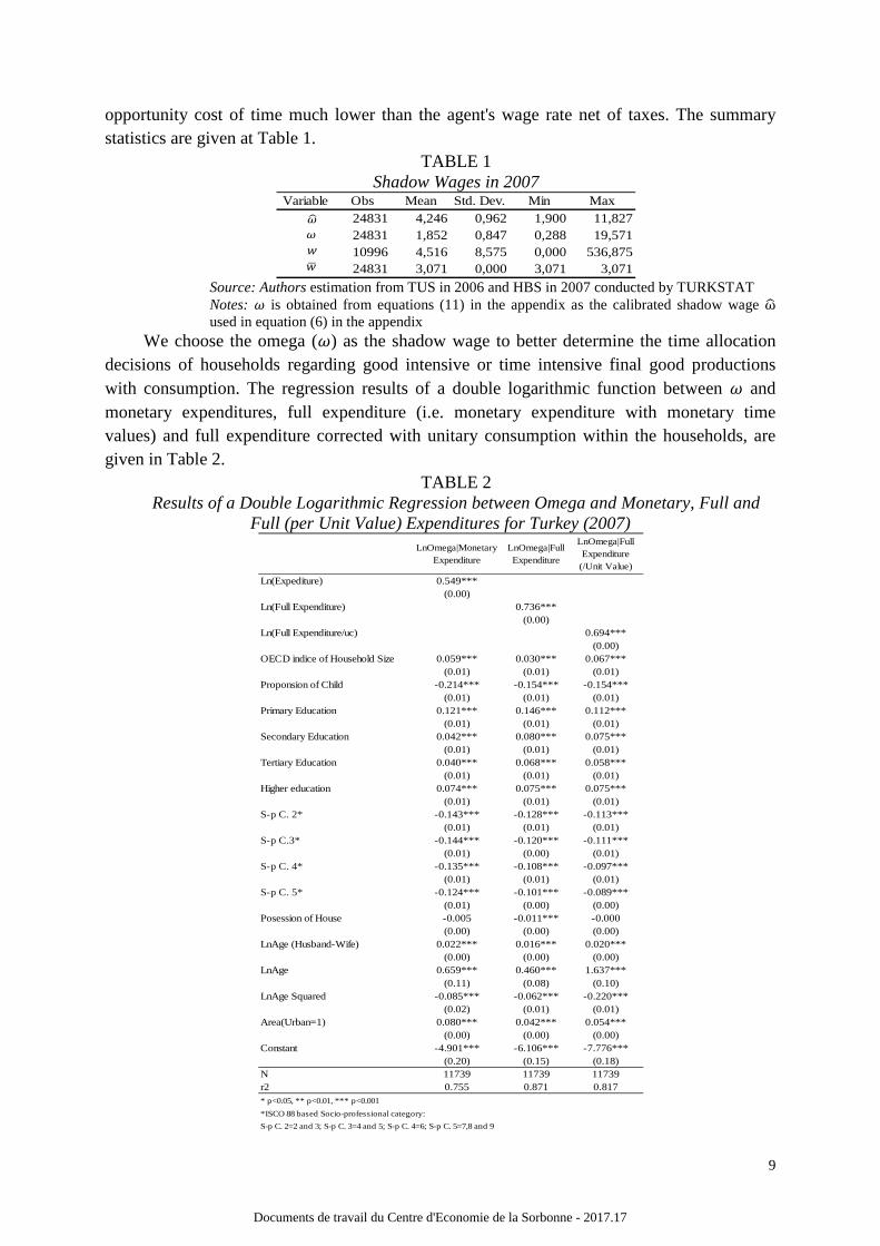
opportunity cost of time much lower than the agent's wage rate net of taxes. The summary statistics are given at Table 1.

TABLE 1 Shadow Wages in 2007

Variable Obs Mean Std. Dev. Min Max24831 4,246 0,962 1,900 11,82724831 1,852 0,847 0,288 19,57110996 4,516 8,575 0,000 536,87524831 3,071 0,000 3,071 3,071

$%

&'

&

$

Source: Authors estimation from TUS in 2006 and HBS in 2007 conducted by TURKSTAT Notes: $ is obtained from equations (11) in the appendix as the calibrated shadow wage ω% used in equation (6) in the appendix

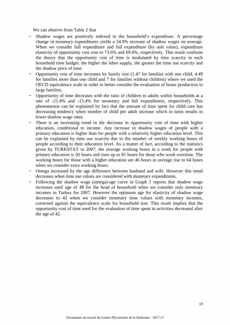
We choose the omega ($) as the shadow wage to better determine the time allocation decisions of households regarding good intensive or time intensive final good productions with consumption. The regression results of a double logarithmic function between $ and monetary expenditures, full expenditure (i.e. monetary expenditure with monetary time values) and full expenditure corrected with unitary consumption within the households, are given in Table 2.

TABLE 2 Results of a Double Logarithmic Regression between Omega and Monetary, Full and

Full (per Unit Value) Expenditures for Turkey (2007)

Ln(Expediture) 0.549***(0.00)

Ln(Full Expenditure) 0.736***(0.00)

Ln(Full Expenditure/uc) 0.694***(0.00)

OECD indice of Household Size 0.059*** 0.030*** 0.067***(0.01) (0.01) (0.01)

Proponsion of Child -0.214*** -0.154*** -0.154***(0.01) (0.01) (0.01)

Primary Education 0.121*** 0.146*** 0.112***(0.01) (0.01) (0.01)

Secondary Education 0.042*** 0.080*** 0.075***(0.01) (0.01) (0.01)

Tertiary Education 0.040*** 0.068*** 0.058***(0.01) (0.01) (0.01)

Higher education 0.074*** 0.075*** 0.075***(0.01) (0.01) (0.01)

S-p C. 2* -0.143*** -0.128*** -0.113***(0.01) (0.01) (0.01)

S-p C.3* -0.144*** -0.120*** -0.111***(0.01) (0.00) (0.01)

S-p C. 4* -0.135*** -0.108*** -0.097***(0.01) (0.01) (0.01)

S-p C. 5* -0.124*** -0.101*** -0.089***(0.01) (0.00) (0.00)

Posession of House -0.005 -0.011*** -0.000(0.00) (0.00) (0.00)

LnAge (Husband-Wife) 0.022*** 0.016*** 0.020***(0.00) (0.00) (0.00)

LnAge 0.659*** 0.460*** 1.637***(0.11) (0.08) (0.10)

LnAge Squared -0.085*** -0.062*** -0.220***(0.02) (0.01) (0.01)

Area(Urban=1) 0.080*** 0.042*** 0.054***(0.00) (0.00) (0.00)

Constant -4.901*** -6.106*** -7.776***(0.20) (0.15) (0.18)

N 11739 11739 11739r2 0.755 0.871 0.817* p<0.05, ** p<0.01, *** p<0.001

*ISCO 88 based Socio-professional category:

S-p C. 2=2 and 3; S-p C. 3=4 and 5; S-p C. 4=6; S-p C. 5=7,8 and 9

LnOmega|Monetary Expenditure

LnOmega|Full Expenditure

LnOmega|Full Expenditure (/Unit Value)


10

We can observe from Table 2 that − Shadow wages are positively indexed in the household’s expenditure. A percentage

change in monetary expenditures yields a 54.9% increase of shadow wages on average. When we consider full expenditure and full expenditure (by unit value), expenditure elasticity of opportunity cost rose to 73.6% and 69.4%, respectively. This result confirms the theory that the opportunity cost of time is modulated by time scarcity in each household time budget: the higher the labor supply, the greater the time use scarcity and the shadow price of time.

− Opportunity cost of time increases by family size (1.47 for families with one child, 4.49 for families more than one child and 7 for families without children) where we used the OECD equivalence scale in order to better consider the evaluation of home production in large families.

− Opportunity of time decreases with the ratio of children to adults within households at a rate of -21.4% and -15.4% for monetary and full expenditures, respectively. This phenomenon can be explained by fact that the amount of time spent for child care has decreasing tendency when number of child per adult increase which in turns results in lower shadow wage rates.

− There is an increasing trend in the decrease in opportunity cost of time with higher education, conditional to income. Any increase in shadow wages of people with a primary education is higher than for people with a relatively higher education level. This can be explained by time use scarcity due to the number of weekly working hours of people according to their education level. As a matter of fact, according to the statistics given by TURKSTAT in 2007, the average working hours in a week for people with primary education is 50 hours and rises up to 81 hours for those who work overtime. The working hours for those with a higher education are 46 hours in average rise to 64 hours when we consider extra working hours.

− Omega increased by the age difference between husband and wife. However this trend decreases when time use values are considered with monetary expenditures.

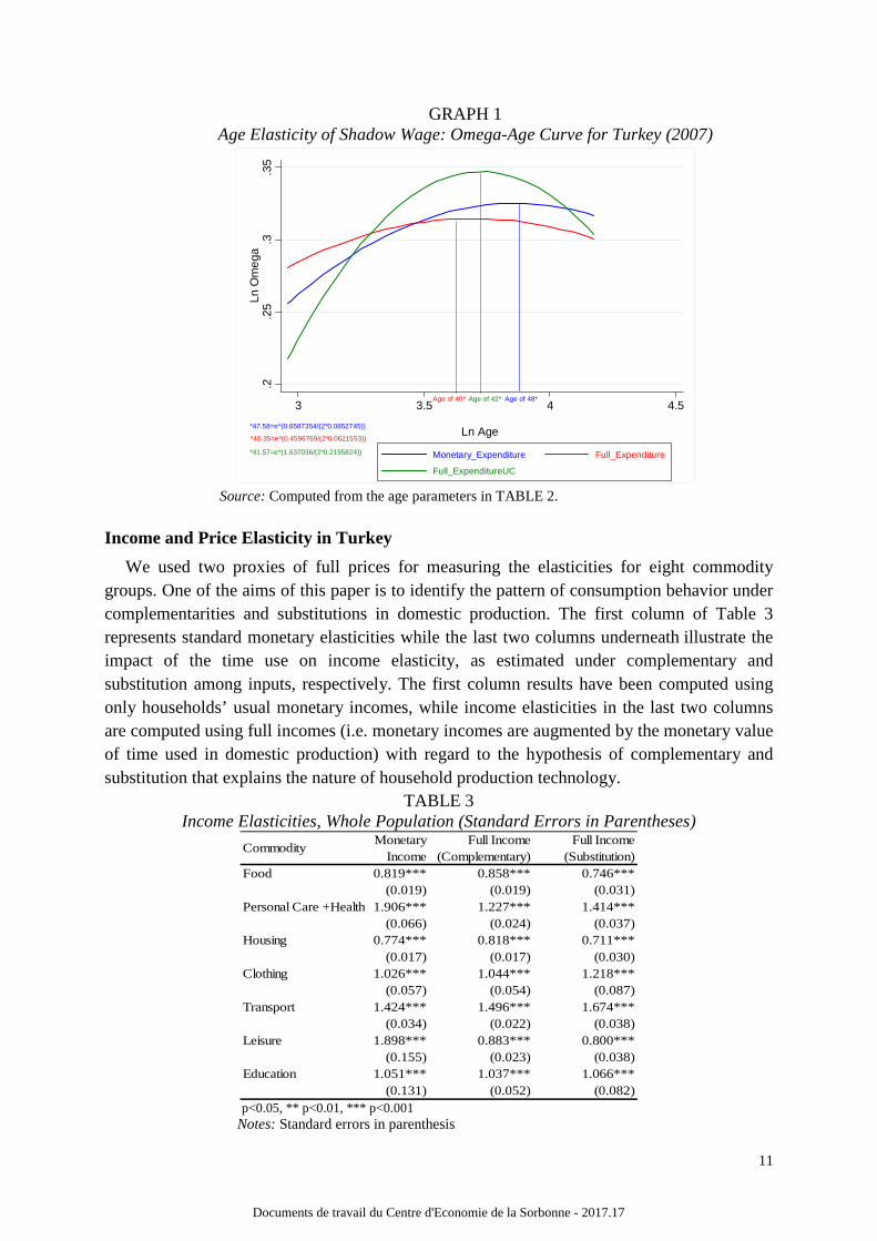
− Following the shadow wage (omega)-age curve in Graph 1 reports that shadow wage increases until age of 48 for the head of household when we consider only monetary incomes in Turkey for 2007. However the optimum age for elasticity of shadow wage decreases to 42 when we consider monetary time values with monetary incomes, corrected against the equivalence scale for household size. This result implies that the opportunity cost of time used for the evaluation of time spent in activities decreased after the age of 42.


11

GRAPH 1 Age Elasticity of Shadow Wage: Omega-Age Curve for Turkey (2007)

Source: Computed from the age parameters in TABLE 2.

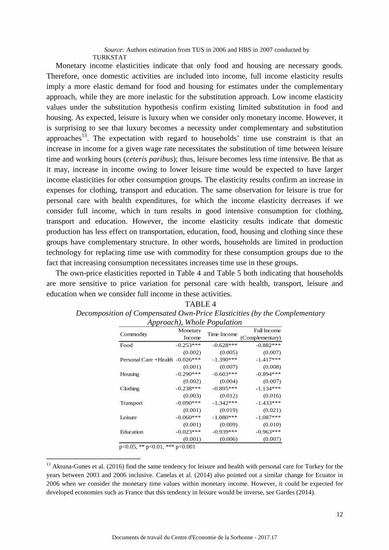
Income and Price Elasticity in Turkey

We used two proxies of full prices for measuring the elasticities for eight commodity groups. One of the aims of this paper is to identify the pattern of consumption behavior under complementarities and substitutions in domestic production. The first column of Table 3 represents standard monetary elasticities while the last two columns underneath illustrate the impact of the time use on income elasticity, as estimated under complementary and substitution among inputs, respectively. The first column results have been computed using only households’ usual monetary incomes, while income elasticities in the last two columns are computed using full incomes (i.e. monetary incomes are augmented by the monetary value of time used in domestic production) with regard to the hypothesis of complementary and substitution that explains the nature of household production technology.

TABLE 3 Income Elasticities, Whole Population (Standard Errors in Parentheses)

Commodity Monetary

IncomeFull Income

(Complementary)Full Income

(Substitution)Food 0.819*** 0.858*** 0.746***

(0.019) (0.019) (0.031)Personal Care +Health 1.906*** 1.227*** 1.414***

(0.066) (0.024) (0.037)Housing 0.774*** 0.818*** 0.711***

(0.017) (0.017) (0.030)Clothing 1.026*** 1.044*** 1.218***

(0.057) (0.054) (0.087)Transport 1.424*** 1.496*** 1.674***

(0.034) (0.022) (0.038)Leisure 1.898*** 0.883*** 0.800***

(0.155) (0.023) (0.038)Education 1.051*** 1.037*** 1.066***

(0.131) (0.052) (0.082) p<0.05, ** p<0.01, *** p<0.001 Notes: Standard errors in parenthesis

.2.2

5.3

.35

Ln O

meg

a

3 3.5 4 4.5

Ln Age

Monetary_Expenditure Full_Expenditure

Full_ExpenditureUC

Age of 48*

*47.58=e^(0.6587354/(2*0.0852745))

Age of 40*

*40.35=e^(0.4596769/(2*0.0621553))

Age of 42*

*41.57=e^(1.637036/(2*0.2195824))


12

Source: Authors estimation from TUS in 2006 and HBS in 2007 conducted by TURKSTAT

Monetary income elasticities indicate that only food and housing are necessary goods. Therefore, once domestic activities are included into income, full income elasticity results imply a more elastic demand for food and housing for estimates under the complementary approach, while they are more inelastic for the substitution approach. Low income elasticity values under the substitution hypothesis confirm existing limited substitution in food and housing. As expected, leisure is luxury when we consider only monetary income. However, it is surprising to see that luxury becomes a necessity under complementary and substitution approaches13. The expectation with regard to households’ time use constraint is that an increase in income for a given wage rate necessitates the substitution of time between leisure time and working hours (ceteris paribus); thus, leisure becomes less time intensive. Be that as it may, increase in income owing to lower leisure time would be expected to have larger income elasticities for other consumption groups. The elasticity results confirm an increase in expenses for clothing, transport and education. The same observation for leisure is true for personal care with health expenditures, for which the income elasticity decreases if we consider full income, which in turn results in good intensive consumption for clothing, transport and education. However, the income elasticity results indicate that domestic production has less effect on transportation, education, food, housing and clothing since these groups have complementary structure. In other words, households are limited in production technology for replacing time use with commodity for these consumption groups due to the fact that increasing consumption necessitates increases time use in these groups.

The own-price elasticities reported in Table 4 and Table 5 both indicating that households are more sensitive to price variation for personal care with health, transport, leisure and education when we consider full income in these activities.

TABLE 4 Decomposition of Compensated Own-Price Elasticities (by the Complementary

Approach), Whole Population

Commodity Monetary

IncomeTime Income

Full Income (Complementary)

Food -0.253*** -0.628*** -0.882***(0.002) (0.005) (0.007)

Personal Care +Health -0.026*** -1.390*** -1.417***(0.001) (0.007) (0.008)

Housing -0.290*** -0.603*** -0.894***(0.002) (0.004) (0.007)

Clothing -0.238*** -0.895*** -1.134***(0.003) (0.012) (0.016)

Transport -0.090*** -1.342*** -1.433***(0.001) (0.019) (0.021)

Leisure -0.060*** -1.080*** -1.087***(0.001) (0.009) (0.010)

Education -0.023*** -0.939*** -0.963***(0.001) (0.006) (0.007)

p<0.05, ** p<0.01, *** p<0.001

13 Aktuna-Gunes et al. (2016) find the same tendency for leisure and health with personal care for Turkey for the years between 2003 and 2006 inclusive. Canelas et al. (2014) also pointed out a similar change for Ecuator in 2006 when we consider the monetary time values within monetary income. However, it could be expected for developed economies such as France that this tendency in leisure would be inverse, see Gardes (2014).


13

Notes: Standard errors in parenthesis Source: Authors estimation from TUS in 2006 and HBS in 2007 conducted by TURKSTAT

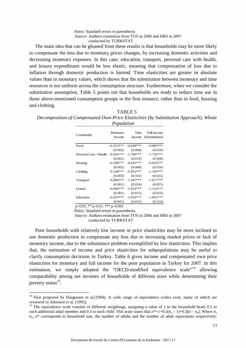
The main idea that can be gleaned from these results is that households may be more likely to compensate the loss due to monetary prices changes, by increasing domestic activities and decreasing monetary expenses. In this case, education, transport, personal care with health, and leisure expenditures would be less elastic, meaning that compensation of loss due to inflation through domestic production is limited. Time elasticities are greater in absolute values than in monetary values, which shows that the substitution between monetary and time resources is not uniform across the consumption structure. Furthermore, when we consider the substitution assumption, Table 5 points out that households are ready to reduce time use in those above-mentioned consumption groups in the first instance, rather than in food, housing and clothing.

TABLE 5 Decomposition of Compensated Own-Price Elasticities (by Substitution Approach), Whole

Population

Commodity Monetary

IncomeTime

IncomeFull Income

(Substitutiary)

Food -0.253*** -0.630*** -0.883***(0.002) (0.008) (0.010)

Personal Care +Health -0.026*** -1.706*** -1.732***(0.001) (0.019) (0.020)

Housing -0.290*** -0.645*** -0.935***(0.002) (0.008) (0.010)

Clothing -0.238*** -0.955*** -1.193***(0.003) (0.022) (0.025)

Transport -0.090*** -1.587*** -1.677***(0.001) (0.024) (0.025)

Leisure -0.060*** -1.052*** -1.112***(0.001) (0.015) (0.016)

Education -0.023*** -1.032*** -1.055***(0.001) (0.013) (0.014)

p<0.05, ** p<0.01, *** p<0.001 Notes: Standard errors in parenthesis. Source: Authors estimation from TUS in 2006 and HBS in 2007 conducted by TURKSTAT

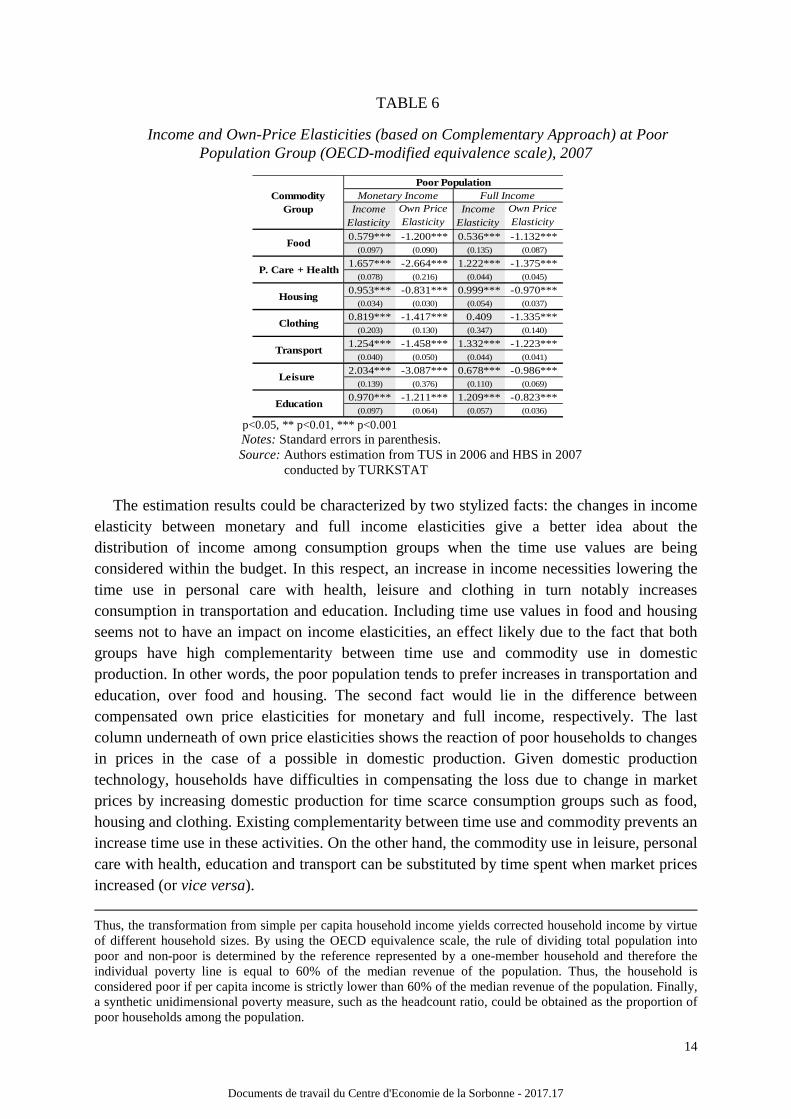
Poor households with relatively low income or price elasticities may be more inclined to

use domestic production to compensate any loss due to increasing market prices or lack of monetary income, due to the subsistence problem exemplified by low elasticities. This implies that, the estimation of income and price elasticities for subpopulations may be useful to clarify consumption decisions in Turkey. Table 6 gives income and compensated own price elasticities for monetary and full income for the poor population in Turkey for 2007. In this estimation, we simply adopted the “OECD-modified equivalence scale”14 allowing comparability among net incomes of households of different sizes while determining their poverty status15.

14 First proposed by Haagenars et al.(1994). A wide range of equivalence scales exist, many of which are reviewed in Atkinson et al. (1995). 15 The equivalence scale consists of different weightings, assigning a value of 1 to the household head, 0.5 to each additional adult member and 0.3 to each child. This scale states that n*=1+0.5(na – 1)+0.3(n – na); Where n, na, n* corresponds to household size, the number of adults and the number of adult equivalents respectively.


14

TABLE 6

Income and Own-Price Elasticities (based on Complementary Approach) at Poor Population Group (OECD-modified equivalence scale), 2007

Income Elasticity

Own Price Elasticity

Income Elasticity

Own Price Elasticity

0.579*** -1.200*** 0.536*** -1.132***(0.097) (0.090) (0.135) (0.087)

1.657*** -2.664*** 1.222*** -1.375***(0.078) (0.216) (0.044) (0.045)

0.953*** -0.831*** 0.999*** -0.970***(0.034) (0.030) (0.054) (0.037)

0.819*** -1.417*** 0.409 -1.335***(0.203) (0.130) (0.347) (0.140)

1.254*** -1.458*** 1.332*** -1.223***(0.040) (0.050) (0.044) (0.041)

2.034*** -3.087*** 0.678*** -0.986***(0.139) (0.376) (0.110) (0.069)

0.970*** -1.211*** 1.209*** -0.823***(0.097) (0.064) (0.057) (0.036)

Food

P. Care + Health

Poor PopulationMonetary Income Full IncomeCommodity

Group

Housing

Clothing

Transport

Leisure

Education

p<0.05, ** p<0.01, *** p<0.001 Notes: Standard errors in parenthesis.

Source: Authors estimation from TUS in 2006 and HBS in 2007 conducted by TURKSTAT

The estimation results could be characterized by two stylized facts: the changes in income elasticity between monetary and full income elasticities give a better idea about the distribution of income among consumption groups when the time use values are being considered within the budget. In this respect, an increase in income necessities lowering the time use in personal care with health, leisure and clothing in turn notably increases consumption in transportation and education. Including time use values in food and housing seems not to have an impact on income elasticities, an effect likely due to the fact that both groups have high complementarity between time use and commodity use in domestic production. In other words, the poor population tends to prefer increases in transportation and education, over food and housing. The second fact would lie in the difference between compensated own price elasticities for monetary and full income, respectively. The last column underneath of own price elasticities shows the reaction of poor households to changes in prices in the case of a possible in domestic production. Given domestic production technology, households have difficulties in compensating the loss due to change in market prices by increasing domestic production for time scarce consumption groups such as food, housing and clothing. Existing complementarity between time use and commodity prevents an increase time use in these activities. On the other hand, the commodity use in leisure, personal care with health, education and transport can be substituted by time spent when market prices increased (or vice versa).

Thus, the transformation from simple per capita household income yields corrected household income by virtue of different household sizes. By using the OECD equivalence scale, the rule of dividing total population into poor and non-poor is determined by the reference represented by a one-member household and therefore the individual poverty line is equal to 60% of the median revenue of the population. Thus, the household is considered poor if per capita income is strictly lower than 60% of the median revenue of the population. Finally, a synthetic unidimensional poverty measure, such as the headcount ratio, could be obtained as the proportion of poor households among the population.


15

Table 7 reports income and own price elasticity results by age, in Turkey for 2007. When we look at the income elasticity results based on monetary and full income, we can observe that there are few changes in food, housing, clothing, transport and education while personal care with health and leisure show large changes across all age cohorts. Income elasticity results for all age groups indicate that food and housing are the both necessities. Clothing is a necessity for the youth population (15-24). Furthermore, personal care with health, leisure and transportation are luxuries for all populations and they take the largest values for the youth population (15-24), while they gradually decrease by age. Personal care with health and leisure are again a source of working time which leads to an increase in consumption of housing, clothing and transportation for the age cohort of 35-44; while food and transportation are the source of a similar increase for adults between ages 45 to 54.

TABLE 7

Income and Own-Price Elasticities by Age Group (based on Complementary Approach), 2007

Income Elasticity

Own Price

Elasticity

Income Elasticity

Own Price

Elasticity

Income Elasticity

Own Price

Elasticity

Income Elasticity

Own Price

Elasticity

Income Elasticity

Own Price

Elasticity

Income Elasticity

Own Price

Elasticity

Income Elasticity

Own Price

Elasticity 0.873*** -0.897*** 2.245*** -3.483*** 0.725*** -0.883*** 0.934*** -1.128*** 1.518*** -1.894*** 2.236*** -3.929*** 1.152*** -1.248***

(0.035) (0.027) (0.189) (0.431) (0.022) (0.030) (0.074) (0.052) (0.066) (0.060) (0.535) (1.146) (0.039) (0.046)

0.862*** -0.902*** 1.284*** -1.587*** 0.782*** -0.937*** 0.927*** -1.091*** 1.521*** -1.559*** 0.930*** -1.130*** 1.069*** -0.963***(0.034) (0.019) (0.029) (0.041) (0.029) (0.025) (0.083) (0.045) (0.046) (0.033) (0.044) (0.036) (0.026) (0.016)

0.785*** -0.904*** 1.825*** -2.589*** 0.781*** -0.867*** 1.023*** -1.241*** 1.388*** -1.675*** 1.865*** -3.237*** 1.134*** -1.337***(0.025) (0.020) (0.059) (0.118) (0.018) (0.018) (0.058) (0.041) (0.052) (0.044) (0.121) (0.248) (0.034) (0.039)

0.795*** -0.889*** 1.207*** -1.392*** 0.856*** -0.944*** 1.183*** -1.173*** 1.380*** -1.444*** 0.862*** -1.123*** 1.049*** -0.949***(0.025) (0.015) (0.019) (0.021) (0.023) (0.017) (0.065) (0.035) (0.035) (0.025) (0.027) (0.025) (0.018) (0.009)

0.831*** -0.859*** 1.877*** -2.708*** 0.795*** -0.813*** 0.993*** -1.189*** 1.401*** -1.637*** 2.011*** -3.257*** 1.002*** -1.255***(0.020) (0.014) (0.047) (0.064) (0.016) (0.013) (0.049) (0.030) (0.036) (0.014) (0.087) (0.166) (0.058) (0.040)

0.893*** -0.872*** 1.222*** -1.416*** 0.858*** -0.882*** 1.012*** -1.142*** 1.494*** -1.432*** 0.893*** -1.120*** 0.965*** -0.969***(0.022) (0.012) (0.015) (0.015) (0.020) (0.012) (0.057) (0.028) (0.030) (0.006) (0.016) (0.012) (0.026) (0.012)

0.786*** -0.857*** 1.969*** -2.711*** 0.752*** -0.804*** 1.054*** -1.233*** 1.427*** -1.634*** 1.990*** -2.894*** 1.027*** -1.203***(0.024) (0.017) (0.058) (0.081) (0.020) (0.016) (0.068) (0.041) (0.047) (0.020) (0.101) (0.185) (0.071) (0.049)

0.828*** -0.868*** 1.246*** -1.433*** 0.767*** -0.884*** 1.066*** -1.160*** 1.511*** -1.430*** 0.871*** -1.043*** 1.126*** -0.956***(0.027) (0.015) (0.021) (0.019) (0.024) (0.013) (0.079) (0.037) (0.038) (0.010) (0.021) (0.016) (0.049) (0.024)

0.810*** -0.859*** 1.659*** -2.651*** 0.750*** -0.807*** 1.243*** -1.116*** 1.365*** -1.783*** 1.787*** -2.769*** 1.264*** -1.420***(0.055) (0.031) (0.100) (0.286) (0.033) (0.026) (0.165) (0.072) (0.108) (0.067) (0.140) (0.265) (0.158) (0.171)

0.743*** -0.954*** 1.268*** -1.424*** 0.933*** -0.907*** 1.094*** -1.167*** 1.459*** -1.486*** 0.968*** -0.995*** 1.029*** -0.947***(0.076) (0.035) (0.052) (0.030) (0.068) (0.033) (0.199) (0.081) (0.161) (0.064) (0.058) (0.045) (0.272) (0.122)

0.780*** -0.901*** 1.960*** -3.036*** 0.870*** -0.822*** 0.906*** -1.261*** 1.206*** -1.796*** 2.733*** -3.815*** 1.244* -1.457***(0.076) (0.048) (0.241) (0.362) (0.052) (0.033) (0.163) (0.099) (0.172) (0.126) (0.494) (0.628) (0.539) (0.413)

0.743*** -0.954*** 1.268*** -1.424*** 0.933*** -0.907*** 1.094*** -1.167*** 1.459*** -1.486*** 0.968*** -0.995*** 1.029*** -0.947***(0.076) (0.035) (0.052) (0.030) (0.068) (0.033) (0.199) (0.081) (0.161) (0.064) (0.058) (0.045) (0.272) (0.122)

25-34Monetary

Full Income

Food Leisure Education

15-24Monetary

Full Income

P. Care + Health Housing Clothing Transport

35-44Monetary

Full Income

45-54Monetary

Full Income

55-64Monetary

Full Income

65+Monetary

Full Income

p<0.05, ** p<0.01, *** p<0.001 Notes: Standard errors in parenthesis. Source: Authors estimation from TUS in 2006 and HBS in 2007 conducted by TURKSTAT

The price elasticity results in Table 6 give a clear picture of the reaction to the increase in market prices with respect to the capacity for increased domestic production of households. The both necessities-food and housing- decreased by price for the youngest population, since the domestic production technology for them would be relatively good intensive. This is also true for the population older than 55 years, simply due to the limits in physical capacity for time use16. Therefore, time use substitution for personal care with health and leisure with age is the highest for the youth and older populations simply because they have relatively fewer working hours than middle-aged populations. Thus, they are more capable of increasing time 16 These are the factors influencing the quality and the quantity of domestic production due to increasing constraints in speed of time use, while combining the inputs pertaining to physical performance etc.


16

intensive domestic production in order to compensate for the loss due to price changes. Any increase in the domestic population in education is relatively limited for the populations between the ages of 15-24 and 44-55.

V. Conclusion

Households’ consumption decisions are expected to be determined by two factors, such as the level of discretionary times use and the technology of combining inputs used in domestic production. The degree of complementarity and substitution between the inputs used in domestic production determines the extent of households’ good intensive consumption. Thus, the domestic production technology would determine the time use scarcity in domestic activities. In this respect, the limit of domestic production is analyzed through estimates of demand elasticities for different subpopulations in the way of clarifying the consumption decisions of Turkish households in 2007. To this end, in this present paper we first estimate shadow wage rates in order to later compute the full price values for each household. Full price values can be interpreted as the price of domestic production which can be specified under the assumptions of complementary and substitution following the theory of allocation proposed by Becker (1965). The theoretical specification and the estimation of demand elasticities with estimated shadow wages are done based on the methodology proposed by Gardes (2016). We found that the average estimate of the shadow wage rate in 2007 is 4.24 which is close to the hourly minimum wage of 2007 rate as 3.07 and smaller than the households’ average hourly wage 4.51. Further, we calibrate the estimated shadow wage rate through the utility function which gives an average estimate of 1.85 for Turkey. The 2006 Time Use Survey and 2007 Household Budget Survey for Turkey are used in this estimation. We match the datasets from both surveys by putting forward a new method proposed by Rubin’s (1986) which gives reliable matching results between time use values and monetary expenditure values from both datasets. The main results that can be gleaned from our analysis are as follows: 1. Shadow wages increase for the head of household until the age of 48 in a decreasing trend

(concave shape) when we only consider monetary incomes in Turkey for 2007. However, the optimum age decreases to 42 when we include monetary time values in monetary incomes (i.e. full income) with the equivalence scale on household size. This result implies that the opportunity cost of time used for the valuation of time spent in activities decreases after the age of 42.

2. As expected, shadow wages are positively indexed on the household’s expenditure. A 10% change in monetary expenditures yields a 54.9% increase in shadow wages. However, the consumption elasticity of opportunity cost rose to 69.4% when using full expenditure.

3. An increase in income for the given wage rate necessitates substitution of time between leisure time (and personal care with health time) and working hours (ceteris paribus); thus, domestic production in leisure and personal care with health time becomes less time intensive. Despite this, an increase in income yields larger income elasticities in clothing, transport and education consumption groups.


17

4. Domestic production has less of an effect on the expenditure groups such as transportation, education, food, housing, clothing having complementary structure since the production technology of replacing time use with commodity for these consumption groups, households are limited for these groups in Turkey.

5. On the other hand, inelastic compensated price elasticity results indicate that replacing loss due to inflation by time use is low for education, transport, personal care with health and leisure expenditures since they are already time intensive consumption groups.

6. The poor population in Turkey has a tendency to favor higher consumption in transportation and in education rather than food and housing since poor households experience difficulty in compensating loss due to change in market prices by increasing domestic production for those time scarce consumption groups.

7. Households’ personal care with health and leisure are used as a source of working time, which enables households to increase consumption in housing, clothing and transportation for the age cohort of 35-44 years, while food and transportation for the adults aged between 45 to 54 also increase.

8. The consumption amounts for the necessities of food and housing for the young population between ages 15-24 and for the group of the population older than 55 decreases due to inflation due to the fact that those groups are more constrained in combining technology used in domestic production, This is due to a lack of knowledge regarding combining technology for younger people; while for older people, it is due to physical limitations.

9. Therefore, substitution of time use with commodity in personal care with health and leisure groups took the highest values for youth and older populations due to the fact that they possess relatively fewer working hours than middle aged populations. Therefore, they are more able to increase time intensive domestic production in order to compensate for any loss due to price changes. Additionally, an increase in the domestic population taking part in education is relatively limited in the populations with age groups 15-24 and 44-55.

References

Aguiar M.A. and E. Hurst (2007). “Measuring Trends in Leisure: the Allocation of Time over Five Decades.” Quarterly Journal of Economic, vol. 22.3, pp. 969-1006.

Aktuna-Gunes, A.T, F. Gardes and C. Starzec (2016). “Informal Markets, Domestic Production and Demand Elasticities: A Case Study for Turkey”, under revision at Economics Bulletin.

Alpman, A. (2016). “Implementing Rubin's alternative multiple-imputation method for statistical matching in Stata”, Stata Journal, Volume 16,3.

Alpman, A. and F. Gardes (2016). “Welfare Analysis of the Allocation of Time During the Great Recession”, Working Paper, Centre d’Economie de la Sorbonne (CES), 2015.12-ISSN: p.1955-611X.

Atkison, A.B., L. Rainwater and T. M. Smeeding. (1995). “Income Distribution in OECD Countries. Evidence from the Luxembourg Income Study”, OECD Social Policy Studies, No.18.

Baral R., C.D., George and Y. Wen, (2011). “Consumption time in household production: Implications for the goods-time elasticity of substitution”, Economic Letters, Vol.112, pp.138-140


18

Becker, G. (1965). “A Theory of the Allocation of Time”, The Economic Journal, Vol.75, pp.493–517.

Buse, A. (1994). “Evaluating the linearized almost ideal demand system”, American Journal of Agricultural Economics, Vol. 76, pp. 781-793.

Canelas, C., F. Gardes and S. Salazar (2014). “Price and Income Elasticities in LAC Countries: The Importance of Domestic Production”, Working Paper, Centre d’Economie de la Sorbonne (CES), 2014.38 - ISSN:p. 1955-611X. 2014

Chiappori, P. A. and A., Lewbel (2014). “Gary Becker’s A theory of the allocation of time”, Economic Journal, Vol.125, pp.1-8.

Davis, G. C. and W. You (2013). “Estimates of returns to scale, elasticity of substitution, and the thrifty food plan meal poverty rate from a direct household meal production function”, Food Policy, vol. 43, pp. 204–212.

De Vany, A. (1974). “The Revealed Value of Time in Air Travel” The Review of Economics and Statistics, Vol. 56(1), pp.77–82.

De Serpa, A. (1971), “A theory of the economics of time”, Economic Journal, Vol. 81,pp.828-846.

Evans, A. (1972). “On the theory of the valuation and allocation of time”, Scottish Journal of Political Economy,Vol. 19,pp.1-17.

Gardes, F. (2016). “The Estimation of Price Elacticity and the Value of Time in a Domestic Production Framework: An Application on to French Micro-data”, Under revision in Annuals of Economics and Statistics.

Green, R.and J.M. Alston, (1990). “Elasticities in AIDS Models”, American Journal of Agricultural Economics, Vol. 72:2, pp.442-445

Gronau, R. (1986). In Handbook of Labour Economics, O. Ashenfelter and R. Layard (ed), Home production - a survey.1,pp.273-304.

Gronau, R. and D. Hamermesh, (2006). “Time vs. goods: the value of measuring household technologies”, Review of Income and Wealth, Vol. 52, pp.1–16.

Hagenaars, A.K. de Vos and M.A. Zaidi, (1994). Poverty Statistics in the Late 1980s: Research Based on Micro-data, Official Publications of the European Communities. Luxembourg.

Hamermesh, D.S., (2008). “Direct estimates of household production”, Economic Letters, Vol. 98, pp.31–34.

Jara-Diaz, S.R, M.A. Munizaga, P. Greeven and K.W. Axhausen. (2013). “Estimating the value of work and leisure”, ETH E-Collection.

Johnson, M. (1966). “Travel Time and the Price of Leisure”, Western Economic Journal, Spring, pp.135-145.

Mincer, J. (1963), “Market Prices, Opportunity Costs, and Income Effects”. In Measurement in Economics, ed. C. Christ. Stanford, Calif.: Stanford University Press, p.67-82.

Moriarity, C., and F. Scheuren (2003). “A Note on Rubin’s Statistical Matching Using File Concatenation with Adjusted Weights and Multiple Imputations”, Journal of Business & Economic Statistics,Vol. 21, pp. 65−73.

Oort, O. (1969). “The Evaluation of Travelling Time.”, Journal of Transport Economics and Policy, Vol. 3, pp.279-286.

Rubin, D. B. (1986). “Statistical Matching Using File Concatenation with Adjusted Weights and Multiple Imputations”, Journal of Business & Economic Statistics, Vol. 4, pp.87−94.

Rubin, D. B. (1987). Multiple imputation for non-response in surveys, New York: John Wiley & Sons.Small, 1982


19

Appendix

1. Shadow Wages and Individual Full Prices

The opportunity cost of time (as the shadow wage rate) is supposed to be different from

minimum wage rate in the calculation of full prices. To get the value of full prices, we need to know the opportunity cost of time spent. In order to calculate the opportunity cost of time Gardes (2016) supposes a Cobb-Douglas structure both for the utility and the domestic production functions of final goods zi. The optimization program is (household h index is omitted in equations for general cases):

( ),

max i

i ii i

m ti

u Z a zγ= ∏ with i ii i i iz b m tα β= (1)

Let mi be monetary expenditure (pi xi). All the parameters in the equation (1) should be estimated locally (i.e. for each household in the dataset), so that this specification assumes for

each household the constancy of the elasticities (iγ ) of the domestic productions in the utility,

and the elasticities , i iα β of the two factors in the production functions in a neighborhood of

their equilibrium point. Under the full income constraint:

( ) ( )i i w wi

t wt T t Im ω ω+ = + − +∑ (2)

Note that w i di

T t t T− = =∑ and that both the market wage and the shadow wage (ω) appear

in the budget equation17: the shadow wage corresponds to the valuation of time in domestic production, and differs from the market wage w whenever there some imperfection exists in the labor market or if the disutility of labor is smaller for domestic production. In order to estimate the opportunity cost for time the utility function is re-written:

( )

' '

i

i i i ii i i i

i i i i

i i i i

i ii

i i i ii i i

u a

a b m t

m t

Z zγ

α γ β γα γ β γα γ β γ

α γ β γ

=

∑ ∑ ∑ ∑ ⇔

∑ ∑⇔

∏

∏ ∏ ∏ (3)

The weights +,-,

∑ +,-, and

/,-,

∑ /,-, are denoted with the geometric weighted means of the

monetary (0′) and time inputs (1′) on the right hand side of the equation. Deriving the utility over income Y and domestic production time 23 gives the opportunity cost of time:

17 The shadow wage rate is supposed to be constant among all domestic activities- see Gardes (2016): Child care is sometimes considered to be more enjoyable than other domestic activities because it is rationed. We thus suppose that there exists no corner optimum in time allocation among domestic activities.


20

'

'

'

'

'

'

'

'

/

/

'

'

( )

( )d

d d

i i d

i i

d t Ti i

i i Ym

u u t

T t Tu u mY m Y

tm T

mtY

T

Y

ω

β γα γ

β γα γ

εε

∂ ∂ ∂∂ ∂ ∂= =∂ ∂ ∂∂ ∂ ∂

∂∂⇔∂∂

⇔

∑∑

∑∑

(4)

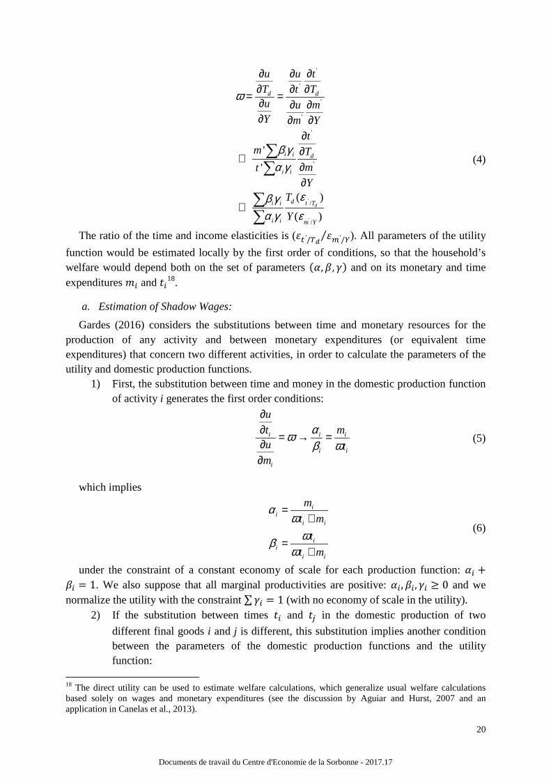
The ratio of the time and income elasticities is (45′/6748′/⁄ ). All parameters of the utility

function would be estimated locally by the first order of conditions, so that the household’s welfare would depend both on the set of parameters ((, ), :) and on its monetary and time expenditures 0� and 1�

18.

a. Estimation of Shadow Wages:

Gardes (2016) considers the substitutions between time and monetary resources for the production of any activity and between monetary expenditures (or equivalent time expenditures) that concern two different activities, in order to calculate the parameters of the utility and domestic production functions.

1) First, the substitution between time and money in the domestic production function of activity i generates the first order conditions:

i i i

i i

i

ut mu tm

αωβ ω

∂∂ = → =∂∂

(5)

which implies

ii

i i

ii

i i

m

t m

t

t m

αω

ωβω

=+

=+

(6)

under the constraint of a constant economy of scale for each production function: (� +

)� = 1. We also suppose that all marginal productivities are positive: (�, )�, :� ≥ 0 and we normalize the utility with the constraint ∑ :� = 1 (with no economy of scale in the utility).

2) If the substitution between times 1� and 1= in the domestic production of two

different final goods i and j is different, this substitution implies another condition between the parameters of the domestic production functions and the utility function:

18 The direct utility can be used to estimate welfare calculations, which generalize usual welfare calculations based solely on wages and monetary expenditures (see the discussion by Aguiar and Hurst, 2007 and an application in Canelas et al., 2013).


21

j i j ii

j i j i j

t m

t m

β αγγ β α

= = (7)

So that

11

1

; i 1ii

i

m

m

αγ γα

= ∀ ≠ (8)

In this respect, the estimation of the opportunity cost of time is directly based on those two steps for all activities i, j:

i j j i i j j im m t tγ γ ωγ ωγ= + − (9)

This could be estimated as a system of >(> − 1) 2⁄ independent equations, calibrating := at

the average full budget share for one good or (n-1)(n-2)/2 equations under the homogeneity constraint of the utility function: ∑ :� = 1. In this system, the opportunity cost of time is over-identified, as well as all := , A > 1. We can also sum equations (9) over j with ∑ := = 1= to

obtain (n-1) independent equations:

( )i i im m T tγ ω ω= + − (10)

This system of equations can be estimated for the whole population, which gives a unique estimate of $ for all households. The estimation can also be performed on subpopulations or by a non-parametric local regression, which affords a set of estimates over the population. The resulting estimates of the opportunity cost of time $ and the parameters := of the utility

function are then used through equations (5-6) to calculate (�, )� for each household. Finally, these estimates of parameters (, ) and : are used to estimate the opportunity cost of time $F for each household in the population through equation (4).

b. Individual Full Prices and Full Price Elasticities

1) The full price pfs can be written for the Cobb-Douglas specification of the domestic

production functions. In fact, t or x can be replaced by tihxih

=pih

ωih

βih

αih which can be

obtained by the first order condition from the consumer optimization program. Thus, writing the quantity of the activity zih in terms, either of t or x, gives:

iα

i ii i

i i

p β1t = z

a ωα

and iβ

i ii i

i i

ωα1x = z

a pβ

(11)

so that the full price for household h becomes: ih ih

s ih ih

α β

f α β ih ihih ih ih

i ih ih

β α1p = p ω +

a α β

(12)

This derivation of $, ( and ) at the individual level allows us to identify the full price for each household where ai is supposed to be constant across the population.

2) For the case of pfc under an assumption of complementarity between the two factors in the domestic technology proxy for the full price of activity i, by the ratio of full expenditure over its monetary component, can be calculated by replacing the estimated shadow wage ($%) rate.


22

ˆ ˆ

cfi h ih ih h ihih

i ih iih

i

(p +ω τ )x ω τ 1= 1+ =

pπ p

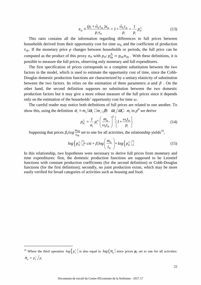
p x p= (13)

This ratio contains all the information regarding differences in full prices between households derived from their opportunity cost for time $F and the coefficient of production G�F. If the monetary price p changes between households or periods, the full price can be

computed as the product of this proxy πih with pih: ��F

�� = ��FH�F . With these definitions, it is

possible to measure the full prices, observing only monetary and full expenditures. The first specification of prices corresponds to a complete substitution between the two

factors in the model, which is used to estimate the opportunity cost of time, since the Cobb-Douglas domestic production functions are characterized by a unitary elasticity of substitution between the two factors. Its relies on the estimation of three parameters: ( and ) . On the other hand, the second definition supposes no substitution between the two domestic production factors but it may give a more robust measure of the full prices since it depends only on the estimation of the households’ opportunity cost for time $.

The careful reader may notice both definitions of full prices are related to one another. To

show this, using the definition ;i i i i i i iim t m t t mα ω β ω ω= + = + in pfs we derive

i

s i

β

f α ih h ihih i

i h ih i

m ω t1p = p 1+

a ω t p

(14)

Supposing that prices )�IJK8,L

5,L set to one for all activities, the relationship yields19,

( ) ( )s cf fihih i ih

ih

mlog p = cst +β log +log p

t

(15)

In this relationship, two hypotheses were necessary to derive full prices from monetary and time expenditures: first, the domestic production functions are supposed to be Leontief functions with constant production coefficients (for the second definition) or Cobb-Douglas functions (for the first definition); secondly, no joint production exists, which may be more easily verified for broad categories of activities such as housing and food.

19 Where the third operation ( )cf

ihlog p is also equal to ( )ihlog π since prices MN set to one for all activities:

cf

ih iih p pπ =


23

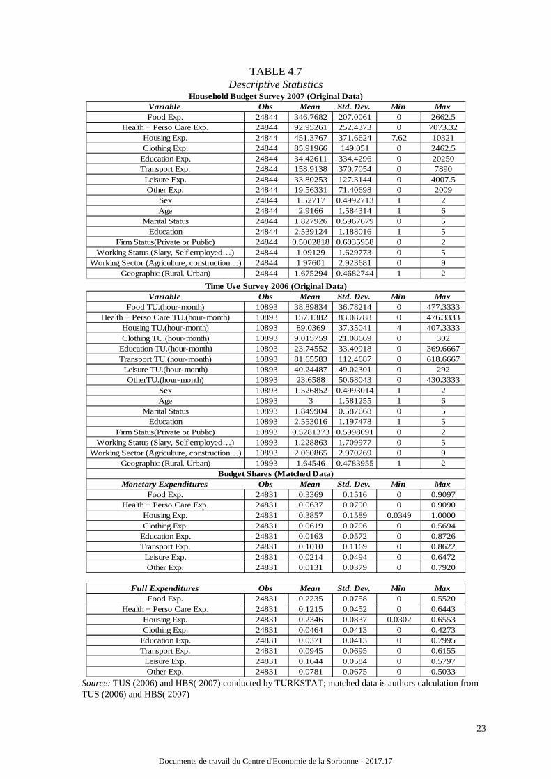
TABLE 4.7 Descriptive Statistics

Variable Obs Mean Std. Dev. Min MaxFood Exp. 24844 346.7682 207.0061 0 2662.5

Health + Perso Care Exp. 24844 92.95261 252.4373 0 7073.32Housing Exp. 24844 451.3767 371.6624 7.62 10321Clothing Exp. 24844 85.91966 149.051 0 2462.5

Education Exp. 24844 34.42611 334.4296 0 20250Transport Exp. 24844 158.9138 370.7054 0 7890Leisure Exp. 24844 33.80253 127.3144 0 4007.5Other Exp. 24844 19.56331 71.40698 0 2009

Sex 24844 1.52717 0.4992713 1 2Age 24844 2.9166 1.584314 1 6

Marital Status 24844 1.827926 0.5967679 0 5Education 24844 2.539124 1.188016 1 5

Firm Status(Private or Public) 24844 0.5002818 0.6035958 0 2Working Status (Slary, Self employed…) 24844 1.09129 1.629773 0 5

Working Sector (Agriculture, construction…) 24844 1.97601 2.923681 0 9Geographic (Rural, Urban) 24844 1.675294 0.4682744 1 2

Variable Obs Mean Std. Dev. Min MaxFood TU.(hour-month) 10893 38.89834 36.78214 0 477.3333

Health + Perso Care TU.(hour-month) 10893 157.1382 83.08788 0 476.3333Housing TU.(hour-month) 10893 89.0369 37.35041 4 407.3333Clothing TU.(hour-month) 10893 9.015759 21.08669 0 302

Education TU.(hour-month) 10893 23.74552 33.40918 0 369.6667Transport TU.(hour-month) 10893 81.65583 112.4687 0 618.6667Leisure TU.(hour-month) 10893 40.24487 49.02301 0 292OtherTU.(hour-month) 10893 23.6588 50.68043 0 430.3333

Sex 10893 1.526852 0.4993014 1 2Age 10893 3 1.581255 1 6

Marital Status 10893 1.849904 0.587668 0 5Education 10893 2.553016 1.197478 1 5

Firm Status(Private or Public) 10893 0.5281373 0.5998091 0 2Working Status (Slary, Self employed…) 10893 1.228863 1.709977 0 5

Working Sector (Agriculture, construction…) 10893 2.060865 2.970269 0 9Geographic (Rural, Urban) 10893 1.64546 0.4783955 1 2

Monetary Expenditures Obs Mean Std. Dev. Min MaxFood Exp. 24831 0.3369 0.1516 0 0.9097

Health + Perso Care Exp. 24831 0.0637 0.0790 0 0.9090Housing Exp. 24831 0.3857 0.1589 0.0349 1.0000Clothing Exp. 24831 0.0619 0.0706 0 0.5694

Education Exp. 24831 0.0163 0.0572 0 0.8726Transport Exp. 24831 0.1010 0.1169 0 0.8622Leisure Exp. 24831 0.0214 0.0494 0 0.6472Other Exp. 24831 0.0131 0.0379 0 0.7920

Full Expenditures Obs Mean Std. Dev. Min MaxFood Exp. 24831 0.2235 0.0758 0 0.5520

Health + Perso Care Exp. 24831 0.1215 0.0452 0 0.6443Housing Exp. 24831 0.2346 0.0837 0.0302 0.6553Clothing Exp. 24831 0.0464 0.0413 0 0.4273

Education Exp. 24831 0.0371 0.0413 0 0.7995Transport Exp. 24831 0.0945 0.0695 0 0.6155Leisure Exp. 24831 0.1644 0.0584 0 0.5797Other Exp. 24831 0.0781 0.0675 0 0.5033

Household Budget Survey 2007 (Original Data)

Time Use Survey 2006 (Original Data)

Budget Shares (Matched Data)

Source: TUS (2006) and HBS( 2007) conducted by TURKSTAT; matched data is authors calculation from TUS (2006) and HBS( 2007)


24

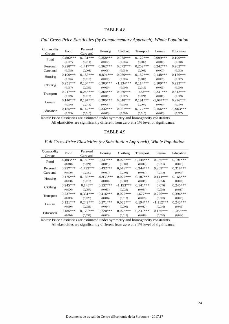
TABLE 4.8

Full Cross-Price Elasticities (by Complementary Approach), Whole Population

Notes: Price elasticities are estimated under symmetry and homogeneity constraints.

All elasticities are significantly different from zero at a 1% level of significance.

TABLE 4.9

Full Cross-Price Elasticities (by Substitution Approach), Whole Population

Notes: Price elasticities are estimated under symmetry and homogeneity constraints. All elasticities are significantly different from zero at a 1% level of significance.

-0,882*** 0,131*** 0,258*** 0,078*** 0,127*** 0,099*** 0,190***(0,007) (0,011) (0,007) (0,006) (0,007) (0,010) (0,008)

0,228*** -1,417*** 0,362*** 0,072*** 0,252*** 0,242*** 0,262***(0,005) (0,008) (0,006) (0,004) (0,005) (0,007) (0,003)

0,190*** 0,153*** -0,894*** 0,069*** 0,157*** 0,148*** 0,176***(0,006) (0,010) (0,007) (0,005) (0,007) (0,009) (0,007)

0,251*** 0,134*** 0,303*** -1,134*** 0,114*** 0,109*** 0,223***(0,017) (0,029) (0,020) (0,016) (0,019) (0,025) (0,016)

0,217*** 0,248*** 0,364*** 0,060*** -1,433*** 0,231*** 0,312***(0,009) (0,012) (0,011) (0,007) (0,021) (0,011) (0,009)

0,140*** 0,197*** 0,285*** 0,048*** 0,191*** -1,087*** 0,226***(0,006) (0,011) (0,008) (0,006) (0,007) (0,010) (0,010)

0,185*** 0,147*** 0,232*** 0,067*** 0,177*** 0,156*** -0,963***(0,009) (0,016) (0,013) (0,008) (0,010) (0,013) (0,007)

Transport

Leisure

Education

Leisure Education

Food

Personal Care and

Housing

Clothing

Commodity Groups

Food Personal Care and

Housing Clothing Transport

-0,883*** 0,150*** 0,237*** 0,075*** 0,144*** 0,086*** 0,191***(0,010) (0,021) (0,011) (0,009) (0,012) (0,015) (0,013)

0,257*** -1,732*** 0,432*** 0,078*** 0,344*** 0,302*** 0,318***(0,009) (0,020) (0,011) (0,008) (0,011) (0,013) (0,009)

0,175*** 0,186*** -0,935*** 0,077*** 0,187*** 0,141*** 0,168***(0,008) (0,019) (0,010) (0,008) (0,011) (0,014) (0,010)

0,245*** 0,148** 0,337*** -1,193*** 0,141*** 0,076 0,245***(0,026) (0,057) (0,033) (0,025) (0,031) (0,039) (0,027)

0,237*** 0,331*** 0,416*** 0,072*** -1,677*** 0,226*** 0,394***(0,013) (0,026) (0,016) (0,012) (0,025) (0,020) (0,013)

0,121*** 0,249*** 0,271*** 0,033*** 0,194*** -1,112*** 0,243***(0,010) (0,023) (0,014) (0,009) (0,012) (0,016) (0,015)

0,185*** 0,179*** 0,220*** 0,073*** 0,231*** 0,166*** -1,055***(0,014) (0,037) (0,023) (0,012) (0,016) (0,020) (0,014)

Transport

Leisure

Education

Leisure Education

Food

Personal Care and

Housing

Clothing

Commodity Groups

Food Personal Care and

Housing Clothing Transport
