Embed Size (px)
Citation preview
1
Decision Support for Lead Time and Demand Variation Reduction
Abstract
Companies undertaking operations improvement in supply chains face many
alternatives. This work seeks to assist practitioners to prioritize improvement actions
by developing analytical expressions for the marginal values of three parameters-- (i)
lead time mean, (ii) lead time variance, and (iii) demand variance– which measure the
marginal cost of an incremental change in a parameter. The relative effectiveness of
reducing the lead time mean versus lead time variance is captured by the ratio ofthe
marginal value of lead time mean to the marginal value of lead time variance. We find
that the value of this ratio strongly depends on whether the lead time mean and
variance are independent or correlated. We illustrate the application of the results with
a numerical example from an industrial setting. These insights can help managers
make tradeoffs among investment decisions to modify demand and supply
characteristics in their supply chain, e.g., by switching suppliers, factory layout, or
investing in information systems.
Keywords
Supply Chain Management, Inventory, Decision Analysis, Lead Time, Marginal Value
1 Introduction
Global competition creates a need for firms to collaborate with supply chain partners
as well as leverage their performance by reducing demand variability(e.g., Lee et al.
[1]; Lee et al. [2]) and supply variability (e.g., Fu and Piplani [3]; Lim [4]). Supply
chain research has proposed a variety of models for potential supply chain
improvements (Ganeshan et al. [5]; Swaminathan and Tayur [6]; Flynn et al. [7]).
However, these models have limitations that restrict them from being fully exploited
by practitioners.
2
The first limitation of existing models is that they target an optimal solution subject to
a given set of supply and demand parameters (Silver [8]). However, in practice
managers can often improve supply chain performance by changing these parameters.
For instance, firms may be able to determine the cost and benefit of switching or
consolidating suppliers, new market development, in-house capacity investment, or
global outsourcing. These initiatives can result in significant changes to lead time as
well as demand and supply variability. An analytical framework is needed for firms to
understand the systematic influence of changed parameters and, consequently, to
make better decisions on how to invest in and adapt to changing supply chain settings.
Second, given limited resources, firms must often choose among alternative
investment decisions, e.g., between focusing on reducing demand variance, lead times,
or lead time varoamce (Smith and Lockamy [9]). These alternatives, such as lead time
mean and variance, are often correlated, and this makes the tradeoff decision more
complicated because the evaluation of only one improvement at a time is insufficient.
For example, Ryu and Lee [10] and Hayya et al. [11] use exponentially distributed
lead times for which means and variances cannot be changed independently.
Furthermore our observations from industry suggest that the relationship between lead
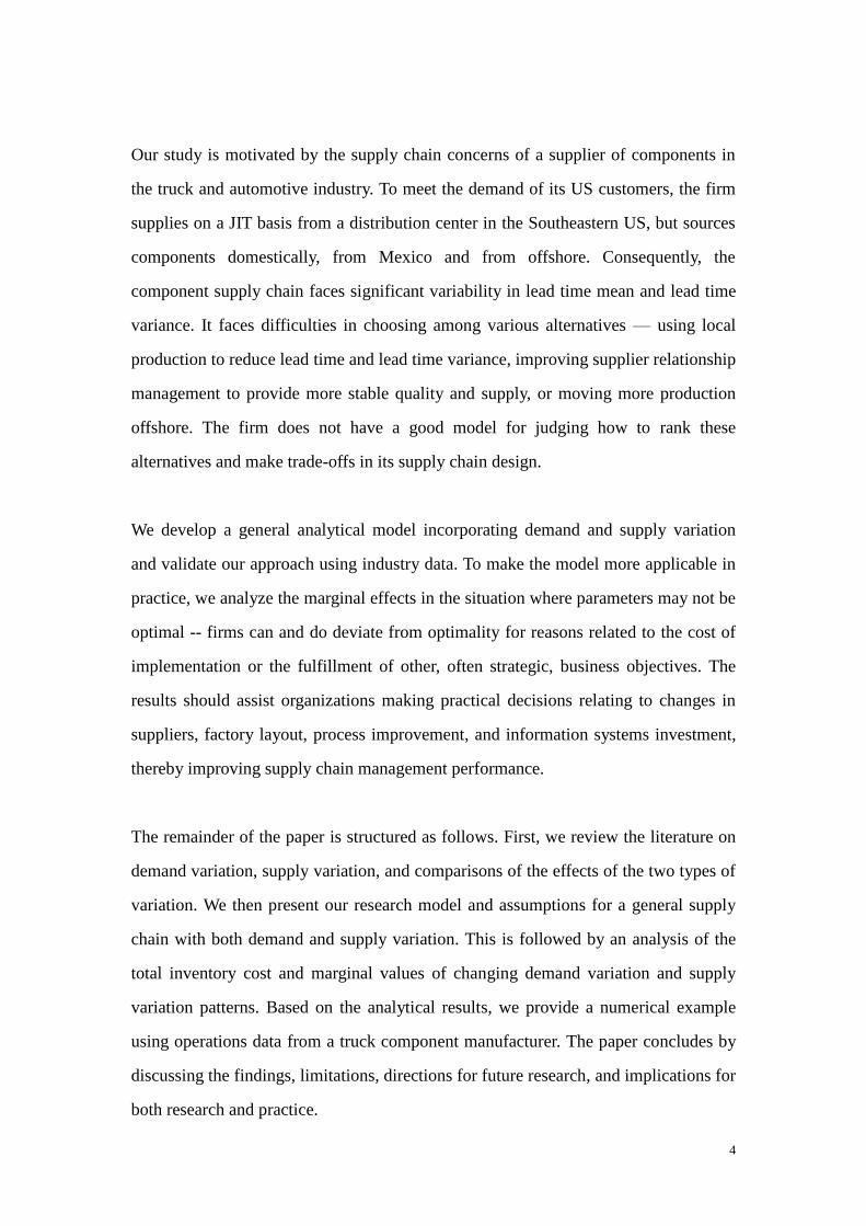
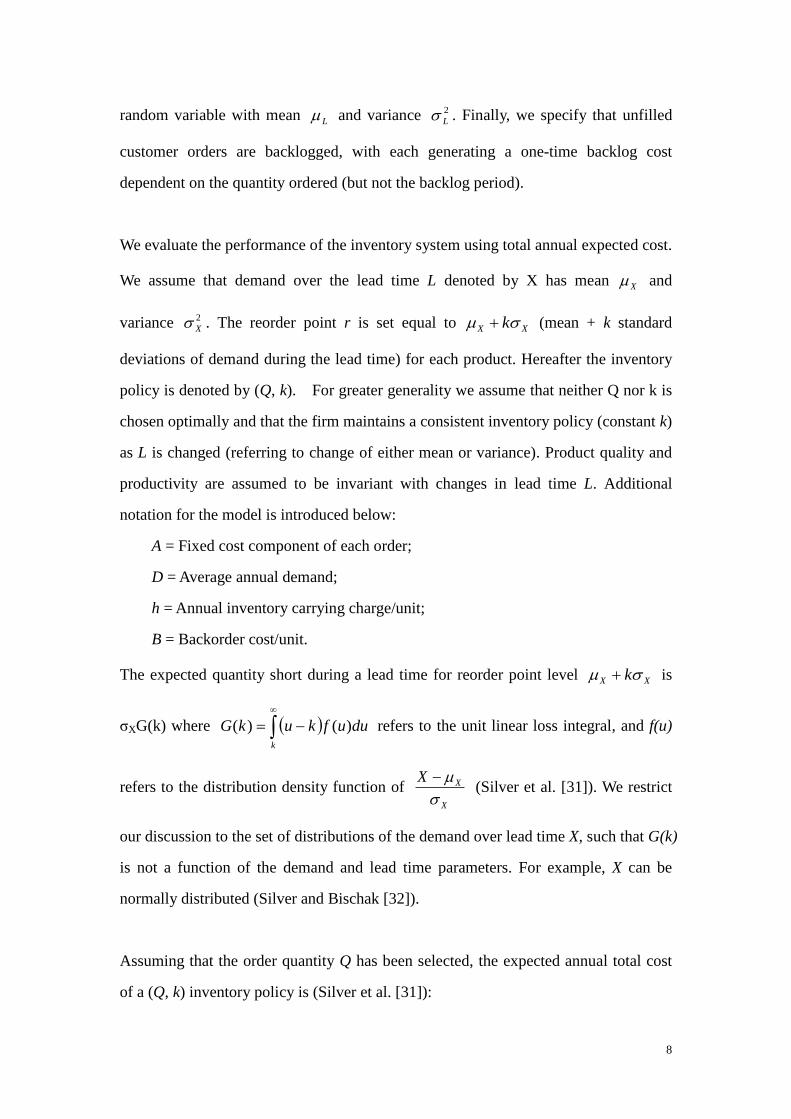
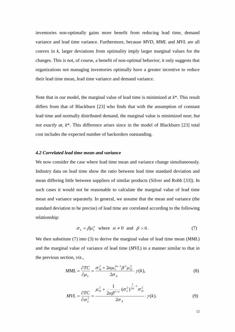
time mean and variance exists in more general settings. The following figure shows
the predicted lead times and standard deviation of the actual lead times of 7653 orders
placed by a major steel distributor on 22 domestic and international suppliers during a
one year period.
3
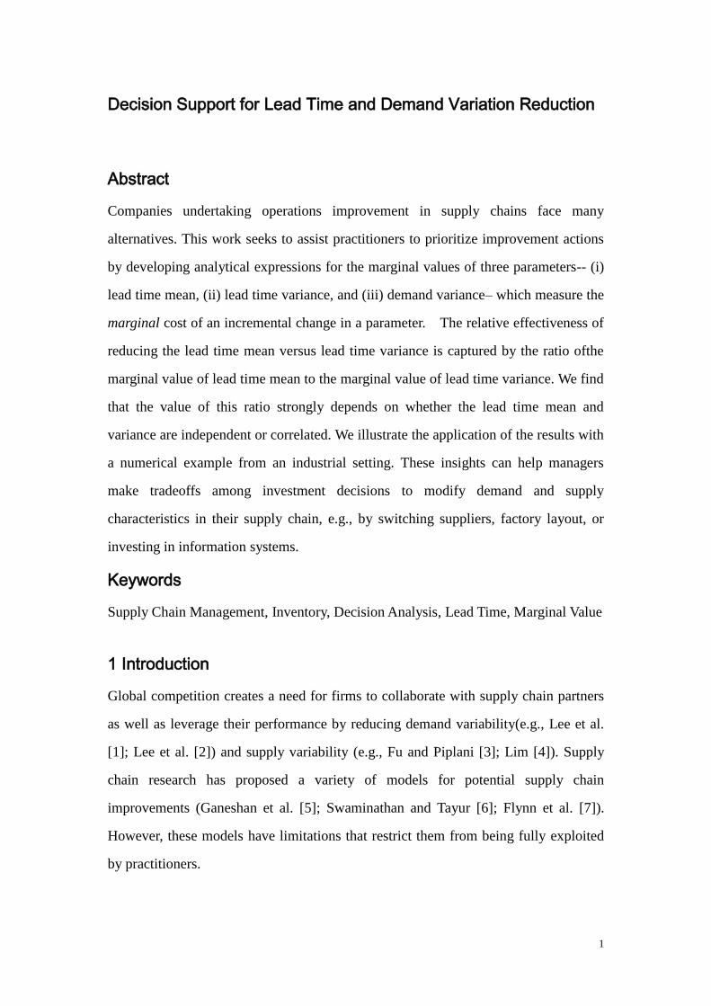
Figure 1: Correlation between lead time mean and variation
Each bubble in Figure 1 represents a particular supplier and a particular predicted lead
time (horizontal axis). The number of orders is indicated by bubble size, and the
standard deviation of the actual lead times is indicated on the vertical axis. The
median coefficient of variation (the standard deviation divided by the predicted lead
time) is 0.30. More than 60% of orders are in categories with coefficient of variation
within the range 0.2-0.4. The figure illustrates positive correlation between the
standard deviation of lead time and expected lead time, both overall, and for a given
supplier. As some products are sourced from multiple suppliers, the figure suggests
that assuming one can adjust the lead time mean and variance separately may not
always be reasonable. A switch to a supplier with shorter lead time may reduce lead
time variance. For other inventory improvements, such as removing outliers,
information sharing or publicizing supplier performance, the mean and variance of the
lead time may be reduced simultaneously.
To bridge these gaps between existing models and practice, this paper aims to help
firms determine how to allocate investment to reduce demand and supply variation.
The study analyzes the marginal effect on cost of reductions in (i) lead time mean, (ii)
lead time vvariance, and (iii) demand variance, in cases where the lead time mean and
variance are either independent or correlated through a functional relationship. We
find the results in the correlated case to be quite different from those in the
independent case.
0
10
20
30
40
50
60
70
0 30 60 90 120 150 180 210
Stan
dar
d d
evi
atio
n o
f le
adti
me
(d
ays)
Predicted Leadtime (days)
Supplier 1 Supplier 2 Supplier 3 Supplier 4 Suppliers 5-22
Bubble size indicatesnumber of orders
4
Our study is motivated by the supply chain concerns of a supplier of components in
the truck and automotive industry. To meet the demand of its US customers, the firm
supplies on a JIT basis from a distribution center in the Southeastern US, but sources
components domestically, from Mexico and from offshore. Consequently, the
component supply chain faces significant variability in lead time mean and lead time
variance. It faces difficulties in choosing among various alternatives — using local
production to reduce lead time and lead time variance, improving supplier relationship
management to provide more stable quality and supply, or moving more production
offshore. The firm does not have a good model for judging how to rank these
alternatives and make trade-offs in its supply chain design.
We develop a general analytical model incorporating demand and supply variation
and validate our approach using industry data. To make the model more applicable in
practice, we analyze the marginal effects in the situation where parameters may not be
optimal -- firms can and do deviate from optimality for reasons related to the cost of
implementation or the fulfillment of other, often strategic, business objectives. The
results should assist organizations making practical decisions relating to changes in
suppliers, factory layout, process improvement, and information systems investment,
thereby improving supply chain management performance.
The remainder of the paper is structured as follows. First, we review the literature on
demand variation, supply variation, and comparisons of the effects of the two types of
variation. We then present our research model and assumptions for a general supply
chain with both demand and supply variation. This is followed by an analysis of the
total inventory cost and marginal values of changing demand variation and supply
variation patterns. Based on the analytical results, we provide a numerical example
using operations data from a truck component manufacturer. The paper concludes by
discussing the findings, limitations, directions for future research, and implications for
both research and practice.
5
2 Literature Review
Supply chain improvement alternatives can be classified into three categories:
reducing demand variability (e.g., Lee et al. [1]), reducing supply variability (e.g.,
Zhang et al. [12]; Song et al. [13]; Qi and Shen [14]) and, reducing demand and
supply variability simultaneously (e.g., Gerchak and Parlar [15]; Das [16]). Existing
literature provides a foundation for our development of a general model for the
analysis of the cost impacts of these categories of variation.
The research on demand variability mainly deals with mechanisms to reduce it and an
evaluation of the benefits of such solutions. According to Lee et al. [1], demand
variability can be moderated through the involvement of point-of-sale (POS) systems,
third party logistics (3PL), and other forms of sharing demand information. Wu et al.
[17] considered the incentives for firms to share their demand information. Hosoda
and Disney [18] studied the setting where only delayed demand information is
available and show that different levels of the supply chain benefit differently from
shorter time delays. These results indicate the potential benefits of methods to reduce
demand variation.
Supply uncertainty has long been identified as a fundamental factor influencing
inventory decisions. Research has focused on inventory models with stochastic lead
times (Bashyam and Fu [19], Bookbinder and Cakanyildirim [20]). In addition to
these works, which are foundational to our current paper, other studies have focused
on methods to reduce supply variability, such as order splitting - the partitioning of an
order between two or more vendors (Hayya et al. [21]).
Two concerns emerge in reducing supply variability: one focuses on reducing the
length of the supply lead time while the other focuses on reducing the variance of the
supply lead time. Focusing on reducing average supply lead time, Blumenfeld et al.
6
[12] developed a queuing model to analyze how manufacturing response time affects
the inventory required at retailers. Fisher et al. [22] considered the problem of
determining retailer replenishment order quantities to minimize the total cost of lost
sales, back orders, and obsolete inventory. The results can be used to quantify the
benefit of lead time reduction and thus select the best replenishment contract.
Blackburn [23] assessed the effect on cost of both increased and decreased
(deterministic) lead time. Recently, Garcia et al. [24] proposed a method for the online
identification of lead times based on a multi-model scheme. Chandra and Grabis [25]
consider the trade-off between benefits of lead-time reduction and increases in
procurement cost. On the other hand, research dealing with the effects of lead time
variance includes Song et al. [13] which demonstrates that ignoring lead time
variability can be costly, but relatively simple heuristics that include lead time
variance perform quite well. Gerchak and Parlar [15] considered the joint
optimization of lead time vvariance, lot size and reorder point in continuous review
inventory models. Wang and Hill [26] investigated the effects of reducing lead time
variance on safety stock when lead time is gamma distributed.
Lastly, several studies compare the relative importance of demand and supply
variability. Paknejad et al. [27], observing the dedication of Japanese manufacturers to
establishing long-term partnerships with their suppliers in order to reduce lead time
variance, concluded that lead time variance was more costly than demand variance.
Vinson [28] observed changes in optimum safety stock and inventory costs using
different combinations of stockout cost, demand variance, lead time mean, and v lead
time variance. He found lead time variance to be more important than either the lead
time mean or the demand variance in explaining inventory cost behavior. However,
Das [16] indicated that cost is more sensitive to lead time mean than it is to lead time
variance. This apparent contradiction stems from the different inventory models and
assumptions employed. More recently, Chopra et al. [29] indicated that there exists a
threshold for service level, with the impacts of lead time variance and lead time mean
differing above and below the threshold. According to He et al. [30], when demand
7
rate is constant, it is the variance and not the mean of lead time that affects the total
relevant cost in a stochastic lead time model.
The existing literature lacks an analysis of the marginal effects of simultaneous
reductions in lead time mean, lead time variance, and demand variance in one general
inventory system. This paper seeks to bridge this gap and help firms determine the
best place to invest efforts in changing demand and supply parameters in their supply
chain setting. We consider the non-optimal setting to provide a more generally
applicable method for practical methods of inventory system improvement.
Furthermore, the existing literature does not consider the situation when lead time
mean and variance are explicitly correlated. The research on correlated lead time
mean and variance is restricted to models in which lead time is exponentially
distributed, e.g. Ryu et al. [10] and Hayya et al. [11]. Thus, they are not able to
compare the correlated case with the case when the mean and variance are
independent, and exponentially distributed lead time is only a special case of
correlated lead time mean and variance. Here we explicitly compare the marginal
values of lead time mean and lead time variance (i.e., the first derivatives of inventory
cost with respect to lead time mean and variance) in the case when the mean and
variance are correlated.
3 Model
We construct a model for a single product with both demand and supply variation.
Demand per unit time is independent and identically distributed with mean D and
variance 2
D . The inventory system is managed by a conventional reorder
quantity/reorder point (Q, r) policy—that is, when the inventory position (inventory
on hand + inventory on order) falls below a level r, an order of size Q is released to
the supplier. For organizations checking their inventory position regularly, with a
short review period, their policy approximates that of a continuous (Q, r) policy.
When the firm places an order, it receives products after a lead time L, which is a
8
random variable with mean L and variance 2
L . Finally, we specify that unfilled
customer orders are backlogged, with each generating a one-time backlog cost
dependent on the quantity ordered (but not the backlog period).
We evaluate the performance of the inventory system using total annual expected cost.
We assume that demand over the lead time L denoted by X has mean X and
variance 2
X . The reorder point r is set equal to XX k (mean + k standard
deviations of demand during the lead time) for each product. Hereafter the inventory
policy is denoted by (Q, k). For greater generality we assume that neither Q nor k is
chosen optimally and that the firm maintains a consistent inventory policy (constant k)
as L is changed (referring to change of either mean or variance). Product quality and
productivity are assumed to be invariant with changes in lead time L. Additional
notation for the model is introduced below:
A = Fixed cost component of each order;
D = Average annual demand;
h = Annual inventory carrying charge/unit;
B = Backorder cost/unit.
The expected quantity short during a lead time for reorder point level XX k is
σXG(k) where duufkukGk
)()(
refers to the unit linear loss integral, and f(u)
refers to the distribution density function of X
XX
(Silver et al. [31]). We restrict
our discussion to the set of distributions of the demand over lead time X, such that G(k)
is not a function of the demand and lead time parameters. For example, X can be
normally distributed (Silver and Bischak [32]).
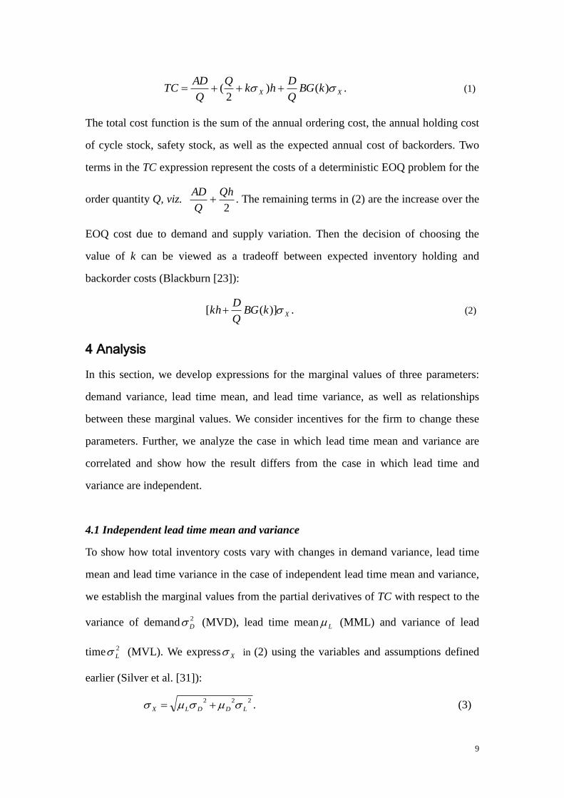
Assuming that the order quantity Q has been selected, the expected annual total cost
of a (Q, k) inventory policy is (Silver et al. [31]):
9
.)()2
( XX kBGQ
Dhk
Q
Q
ADTC (1)
The total cost function is the sum of the annual ordering cost, the annual holding cost
of cycle stock, safety stock, as well as the expected annual cost of backorders. Two
terms in the TC expression represent the costs of a deterministic EOQ problem for the
order quantity Q, viz. 2
Qh
Q
AD . The remaining terms in (2) are the increase over the
EOQ cost due to demand and supply variation. Then the decision of choosing the
value of k can be viewed as a tradeoff between expected inventory holding and
backorder costs (Blackburn [23]):
.)]([ XkBGQ
Dkh (2)
4 Analysis
In this section, we develop expressions for the marginal values of three parameters:
demand variance, lead time mean, and lead time variance, as well as relationships
between these marginal values. We consider incentives for the firm to change these
parameters. Further, we analyze the case in which lead time mean and variance are
correlated and show how the result differs from the case in which lead time and
variance are independent.
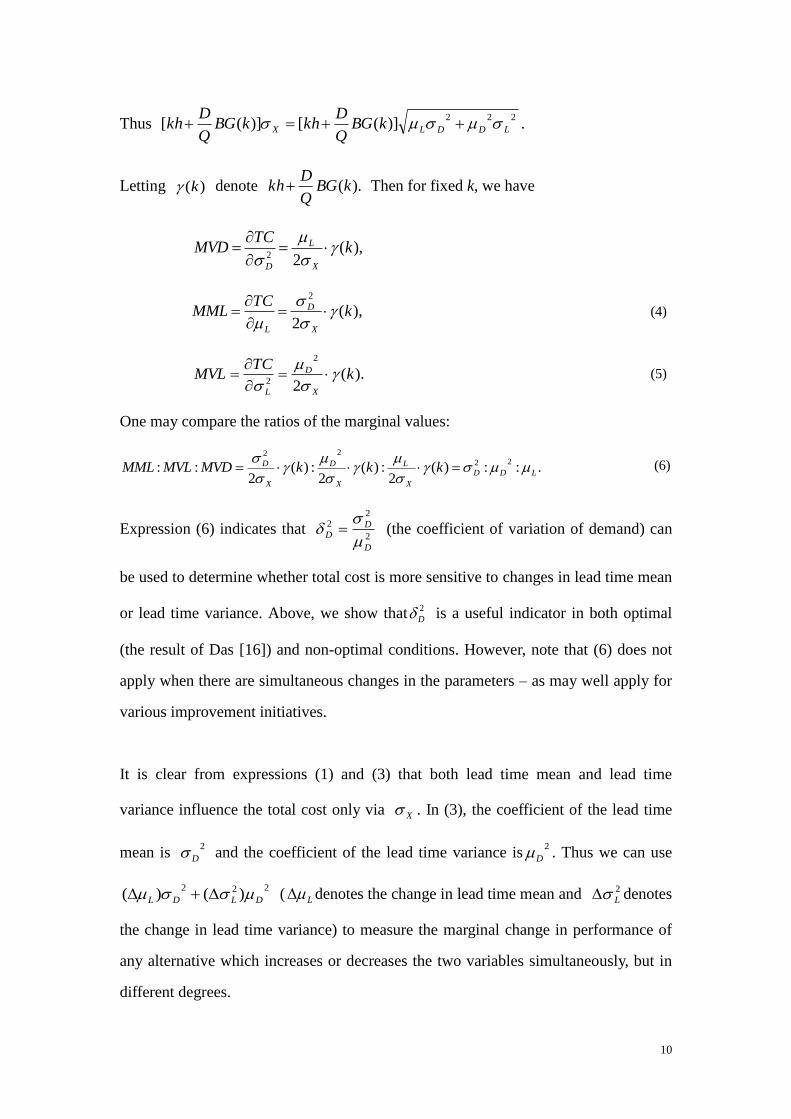
4.1 Independent lead time mean and variance
To show how total inventory costs vary with changes in demand variance, lead time
mean and lead time variance in the case of independent lead time mean and variance,
we establish the marginal values from the partial derivatives of TC with respect to the
variance of demand 2
D (MVD), lead time mean L (MML) and variance of lead
time 2
L (MVL). We express X in (2) using the variables and assumptions defined
earlier (Silver et al. [31]):
.222
LDDLX (3)
10
Thus 222
)]([)]([ LDDLX kBGQ
DkhkBG
Q
Dkh .
Letting )(k denote ).(kBGQ
Dkh
Then for fixed k, we have
),(22
kTC
MVDX
L
D
),(2
2
kTC
MMLX
D
L
(4)
).(2
2
2k
TCMVL
X
D
L
(5)
One may compare the ratios of the marginal values:
.::)(2
:)(2
:)(2
::22
22
LDD
X
L
X
D
X
D kkkMVDMVLMML
(6)
Expression (6) indicates that 2
22
D
DD
(the coefficient of variation of demand) can
be used to determine whether total cost is more sensitive to changes in lead time mean
or lead time variance. Above, we show that 2
D is a useful indicator in both optimal
(the result of Das [16]) and non-optimal conditions. However, note that (6) does not
apply when there are simultaneous changes in the parameters – as may well apply for
various improvement initiatives.
It is clear from expressions (1) and (3) that both lead time mean and lead time
variance influence the total cost only via X . In (3), the coefficient of the lead time
mean is 2
D and the coefficient of the lead time variance is2
D . Thus we can use
222)()( DLDL ( L denotes the change in lead time mean and 2
L denotes
the change in lead time variance) to measure the marginal change in performance of
any alternative which increases or decreases the two variables simultaneously, but in
different degrees.
11
Incentive to Change We now examine some additional properties of the marginal
values. Furthermore, we extend the incentives to improve lead time performance
given by Blackburn [23] to the case of stochastic lead time.
The following proposition shows the effects of the changes of demand variance, lead
time mean and lead time variance on the marginal values of the three, respectively.
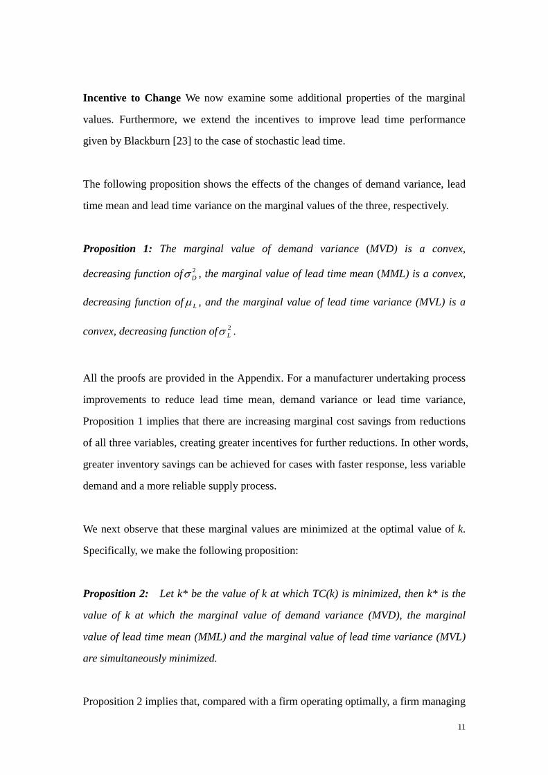
Proposition 1: The marginal value of demand variance (MVD) is a convex,
decreasing function of 2
D , the marginal value of lead time mean (MML) is a convex,
decreasing function of L , and the marginal value of lead time variance (MVL) is a
convex, decreasing function of 2
L .
All the proofs are provided in the Appendix. For a manufacturer undertaking process
improvements to reduce lead time mean, demand variance or lead time variance,
Proposition 1 implies that there are increasing marginal cost savings from reductions
of all three variables, creating greater incentives for further reductions. In other words,
greater inventory savings can be achieved for cases with faster response, less variable
demand and a more reliable supply process.
We next observe that these marginal values are minimized at the optimal value of k.
Specifically, we make the following proposition:
Proposition 2: Let k* be the value of k at which TC(k) is minimized, then k* is the
value of k at which the marginal value of demand variance (MVD), the marginal
value of lead time mean (MML) and the marginal value of lead time variance (MVL)
are simultaneously minimized.
Proposition 2 implies that, compared with a firm operating optimally, a firm managing
12
inventories non-optimally gains more benefit from reducing lead time, demand
variance and lead time variance. Furthermore, because MVD, MML and MVL are all
convex in k, larger deviations from optimality imply larger marginal values for the
changes. This is not, of course, a benefit of non-optimal behavior; it only suggests that
organizations not managing inventories optimally have a greater incentive to reduce
their lead time mean, lead time variance and demand variance.
Note that in our model, the marginal value of lead time is minimized at k*. This result
differs from that of Blackburn [23] who finds that with the assumption of constant
lead time and normally distributed demand, the marginal value is minimized near, but
not exactly at, k*. This difference arises since in the model of Blackburn [23] total
cost includes the expected number of backorders outstanding.
4.2 Correlated lead time mean and variance
We now consider the case where lead time mean and variance change simultaneously.
Industry data on lead time show the ratio between lead time standard deviation and
mean differing little between suppliers of similar products (Silver and Robb [33]). In
such cases it would not be reasonable to calculate the marginal value of lead time
mean and variance separately. In general, we assume that the mean and variance (the
standard deviation to be precise) of lead time are correlated according to the following
relationship:
LL where 0 and 0 . (7)
We then substitute (7) into (3) to derive the marginal value of lead time mean (MML)
and the marginal value of variance of lead time (MVL) in a manner similar to that in
the previous section, viz.,
),(2
2 22122
kTC
MMLX
DLD
L
(8)
).(2
)(2
1 21
2
1
2
/1
2
2k
TCMVL
X
DLD
L
(9)
13
The marginal values include terms additional to those in (4) and (5). When α is
positive, these additional terms are positive, signaling the extra benefits a firm can
gain. When the firm reduces the lead time mean, it simultaneously reduces lead time
variance.
The ratio of the marginal values is as follows,
.22
1)(2
1
2:
2212
21
2
1
22
/1
2122
L
LL
DL
LDM V LMML
(10)
This result is quite different from expression (6). When lead time mean and variance
can be changed independently, the relative effect on cost depends only on the ratio of
demand variance to demand mean. However, when the lead time mean and variance
are correlated, the ratio becomes linear in α and is independent of β. Thus, β, which
may be determined empirically by regressing lead time variance against the mean, has
no bearing on the relative importance of the mean and variance.
Now we consider the validity of Propositions 1 and 2 with correlated lead time mean
and variance. Proposition 2 still holds, as )(k is the only term containing k.
Proposition 1 also holds, provided some constraints are placed on the value of α
(which are sufficient).
Proposition 3: (a) if ]2
1,0( , the marginal value of lead time mean (MML) is a
convex, decreasing function of L ; (b) if ),2
1[ , the marginal value of lead time
variation (MVL) is a convex, decreasing function of 2
L .
When 2
1 , the first and second derivatives of both MML and MVL have the same
sign as in the case in which lead time mean and variance are independent. For other
14
values of α, MML or MVL may not be monotone decreasing. Unlike the case in
which lead time mean and variance are independent, the reduction in total cost may
not increase with the reduction of lead time mean and variance. In fact, as Proposition
4 shows below, critical points exist for lead time mean and variance at which the
monotonicity of marginal values changes.
Proposition 4: (a) For ]1,0( and all 0L , the marginal value of lead time
mean (MML) is a decreasing function of L ; For 0 or 1 , there exists a
critical point *
L at which the monotonicity of MML changes.
(b) For 4
1
and all 2
L , the marginal value of lead time variance (MVL) is a
decreasing function of 2
L ; For 0 or )4
1,0( , there exists a critical point
*2
L at which the monotonicity of MVL changes.
Proposition 4 implies that in the correlated case, evaluating the ‘incentive’ for firms
seeking to improve their inventory performance by reducing the lead time mean or
variance is a more complex function of lead time mean. Specifically, we have the
monotonicity of marginal values as shown in Table 1.
Independent Correlated
Value of Below the critical point Above the critical point
MML Decreasing
0 Increasing Decreasing
]1,0( Decreasing Decreasing
1 Decreasing Increasing
MVL Decreasing
0 Increasing Decreasing
)4/1,0( Decreasing Increasing
4/1
Decreasing Decreasing
Table 1: Changes of monotonicity of marginal values
One may expect decreasing returns at first when seeking to reduce the lead time mean
if the variance is very sensitive to the change of mean (i.e., with large α). On the
15
other hand, firms seeking to reduce lead time variance may obtain decreasing returns
at first if the variance is not very sensitive to the change of mean (with small α).
However, as illustrated by Proposition 1, the incentive for further reductions still
exists for the correlated case in the sense that increasing returns will always be
observed when the mean or variance is small enough. When the mean and variance
are negatively correlated, e.g., the supplier offers slower but more reliable
performance (it is easier for the supplier to deliver on time if it promises a longer lead
time), they should be mindful of decreasing marginal values and potentially negative
marginal values (as seen in the numerical example below) when the mean or variance
is small.
5 Numerical Examples
In this section, we use a numerical example to illustrate the above results in a practical
situation. We consider the case of Springfield Manufacturing, the truck and
automotive component supplier first described in Section 1. In sourcing their
components both in North America and offshore, Springfield’s supply chain has both
demand and lead time (supply) variability. Their main customer—an assembler of
large over-the-road trucks—provides a general forecast of the overall level of
component demand but requires JIT shipments of components of an amount equal to
one or two days’ demand. Springfield must make to stock as these components are
manufactured in Mexico and shipped to a distribution site in the Southeastern US.
We examine the effect of lead time on the cost of managing the inventory for one of
their highest demand truck components. The cost of production and distribution for
the component was $25/unit. Daily demand for the item was about 90 units with a
standard deviation of 28 units (Weekly demand was 450 units with a standard
deviation of 62.6). A normal distribution provided an adequate fit to demand for the
component and no autocorrelation was found in historical data . Production order
quantities (Q) equaled about 4 weeks demand or about 1800 units. The setup cost of a
16
production lot (A) was about $250, and the annual cost of carrying a unit in stock (h)
was $3.75 (or about 15% of the cost of the unit). The penalty cost per unit for a
backorder (B) was estimated to be $25. The sum of supply and production lead time
(also approximately normally distributed) was about 30 days with a standard
deviation of 0.3.
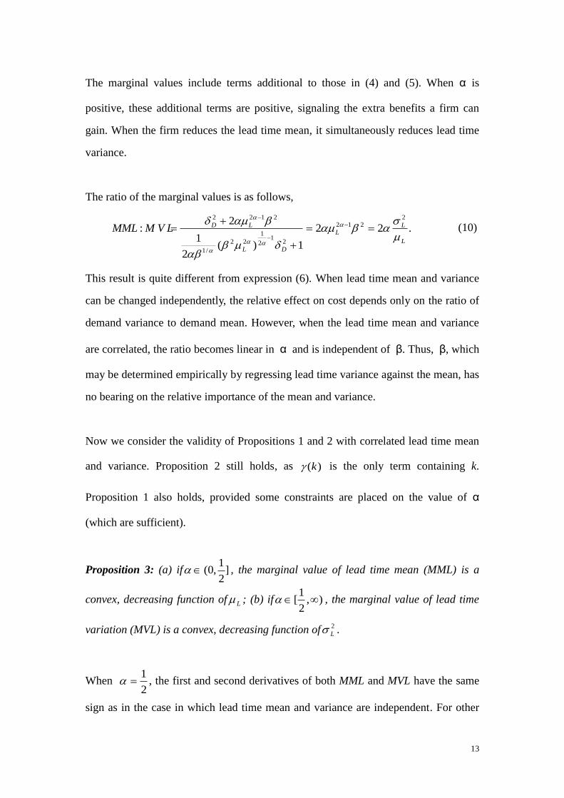
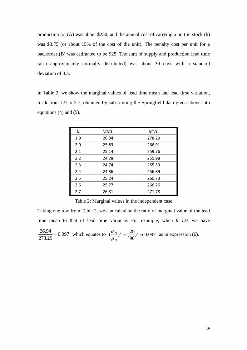
In Table 2, we show the marginal values of lead time mean and lead time variation,
for k from 1.9 to 2.7, obtained by substituting the Springfield data given above into
equations (4) and (5).
k MML MVL
1.9 26.94 278.29
2.0 25.83 266.91
2.1 25.14 259.76
2.2 24.78 255.98
2.3 24.74 255.59
2.4 24.86 256.89
2.5 25.24 260.73
2.6 25.77 266.26
2.7 26.31 271.78
Table 2: Marginal values in the independent case
Taking one row from Table 2, we can calculate the ratio of marginal value of the lead
time mean to that of lead time variance. For example, when k=1.9, we have
097.029.278
94.26 which equates to 097.0)
90
28()( 22
D
D
as in expression (6).
17
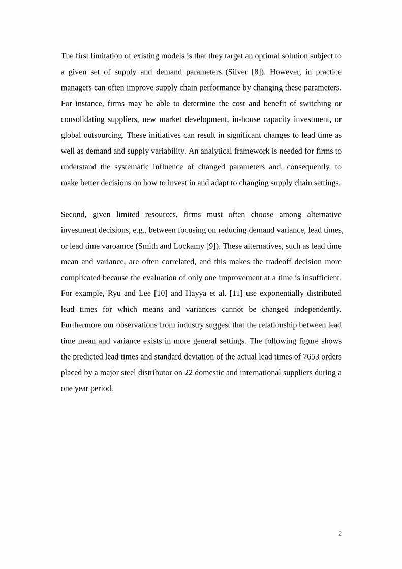
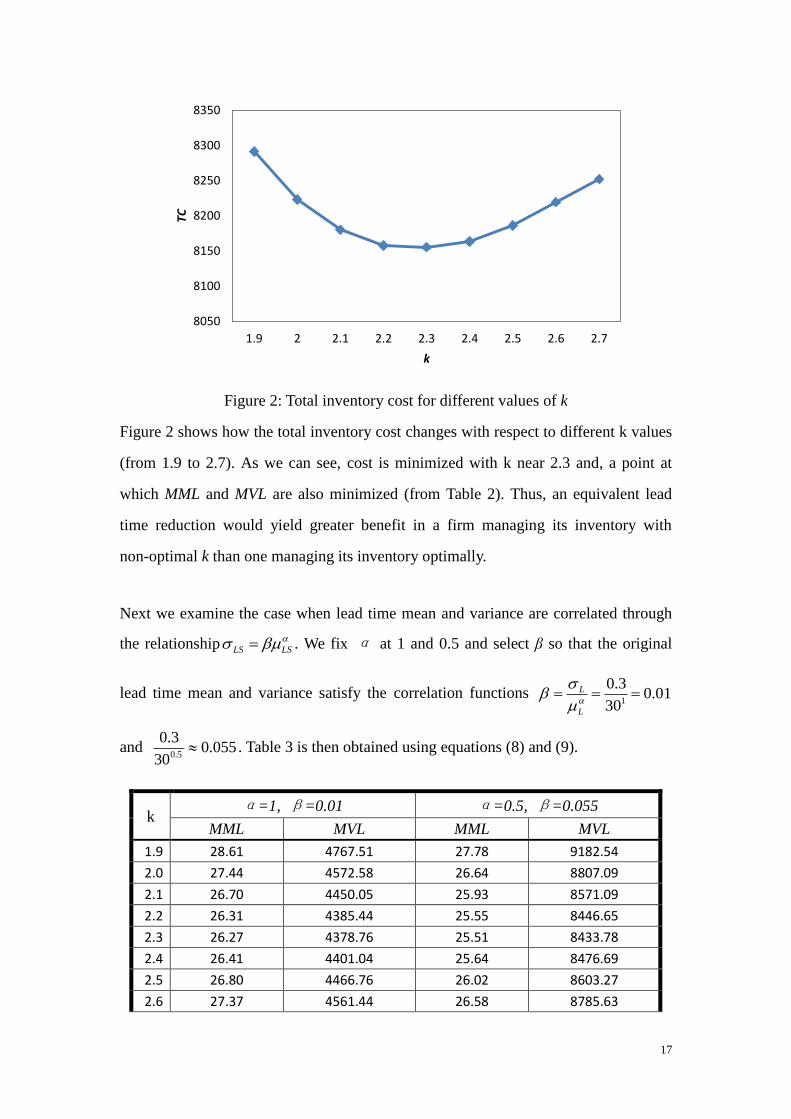
Figure 2: Total inventory cost for different values of k
Figure 2 shows how the total inventory cost changes with respect to different k values
(from 1.9 to 2.7). As we can see, cost is minimized with k near 2.3 and, a point at
which MML and MVL are also minimized (from Table 2). Thus, an equivalent lead
time reduction would yield greater benefit in a firm managing its inventory with
non-optimal k than one managing its inventory optimally.
Next we examine the case when lead time mean and variance are correlated through
the relationship LSLS . We fix α at 1 and 0.5 and select β so that the original
lead time mean and variance satisfy the correlation functions 01.030
3.01
L
L
and 055.030
3.05.0 . Table 3 is then obtained using equations (8) and (9).
k α=1, β=0.01 α=0.5, β=0.055
MML MVL MML MVL
1.9 28.61 4767.51 27.78 9182.54
2.0 27.44 4572.58 26.64 8807.09
2.1 26.70 4450.05 25.93 8571.09
2.2 26.31 4385.44 25.55 8446.65
2.3 26.27 4378.76 25.51 8433.78
2.4 26.41 4401.04 25.64 8476.69
2.5 26.80 4466.76 26.02 8603.27
2.6 27.37 4561.44 26.58 8785.63
8050
8100
8150
8200
8250
8300
8350
1.9 2 2.1 2.2 2.3 2.4 2.5 2.6 2.7
TC
k
18
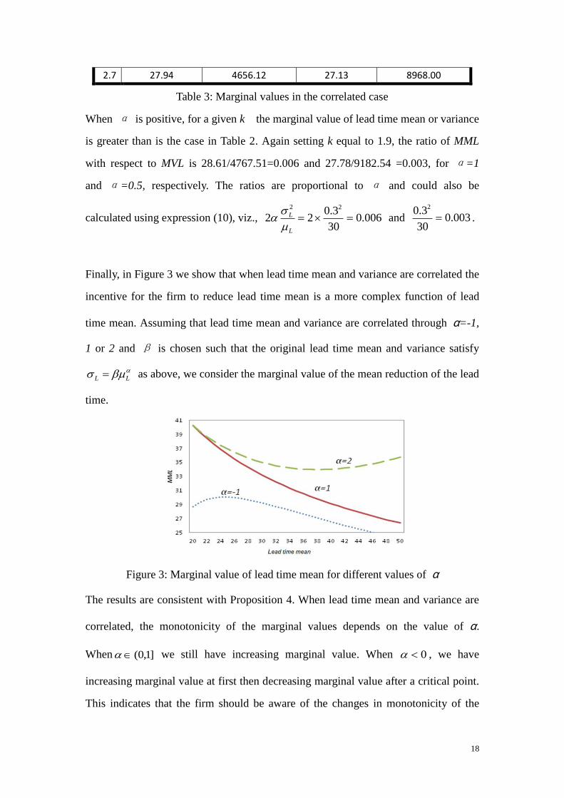
2.7 27.94 4656.12 27.13 8968.00
Table 3: Marginal values in the correlated case
When α is positive, for a given k the marginal value of lead time mean or variance
is greater than is the case in Table 2. Again setting k equal to 1.9, the ratio of MML
with respect to MVL is 28.61/4767.51=0.006 and 27.78/9182.54 =0.003, for α=1
and α=0.5, respectively. The ratios are proportional to α and could also be
calculated using expression (10), viz., 006.030
3.022
22
L
L
and 003.0
30
3.0 2
.
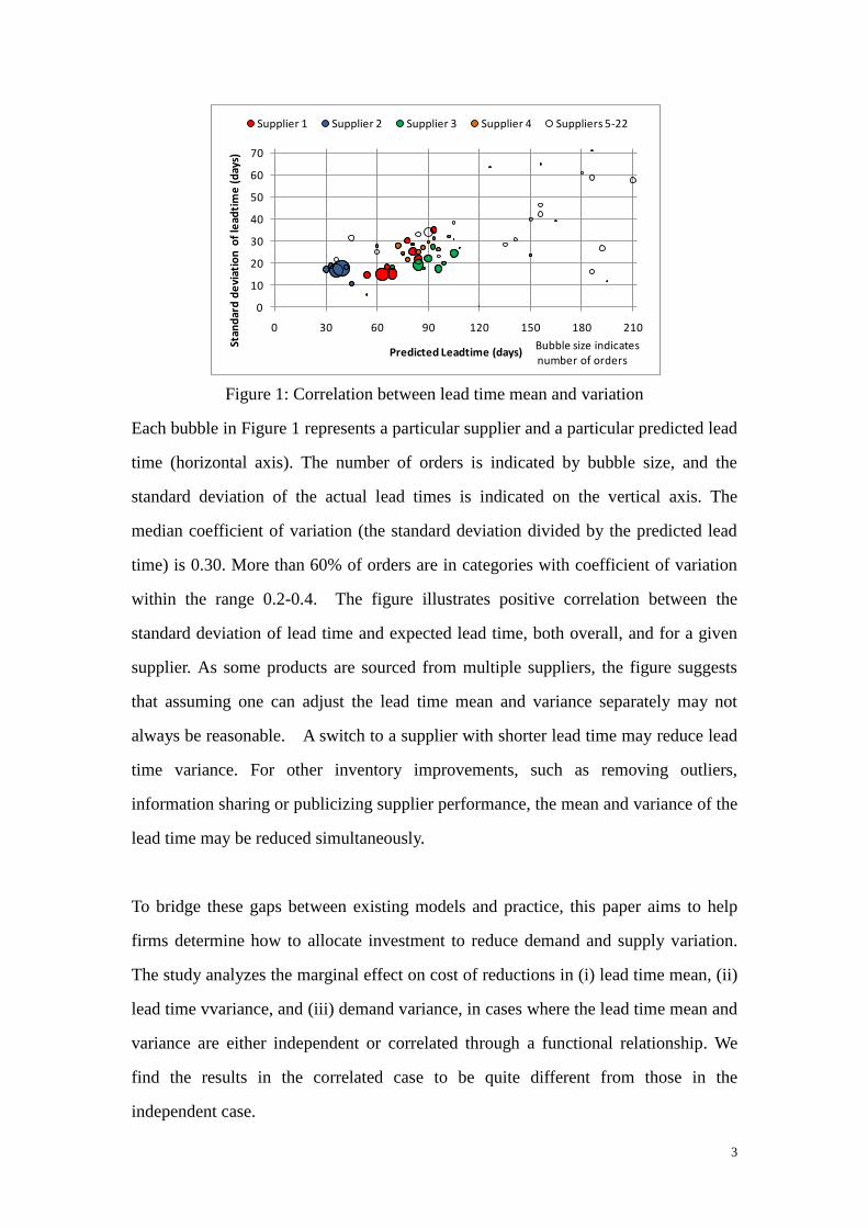
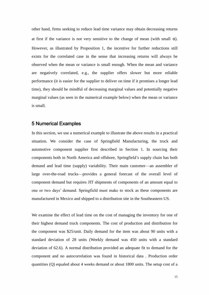
Finally, in Figure 3 we show that when lead time mean and variance are correlated the
incentive for the firm to reduce lead time mean is a more complex function of lead
time mean. Assuming that lead time mean and variance are correlated through α=-1,
1 or 2 and β is chosen such that the original lead time mean and variance satisfy
LL as above, we consider the marginal value of the mean reduction of the lead
time.
Figure 3: Marginal value of lead time mean for different values of α
The results are consistent with Proposition 4. When lead time mean and variance are
correlated, the monotonicity of the marginal values depends on the value of α.
When ]1,0( we still have increasing marginal value. When 0 , we have
increasing marginal value at first then decreasing marginal value after a critical point.
This indicates that the firm should be aware of the changes in monotonicity of the
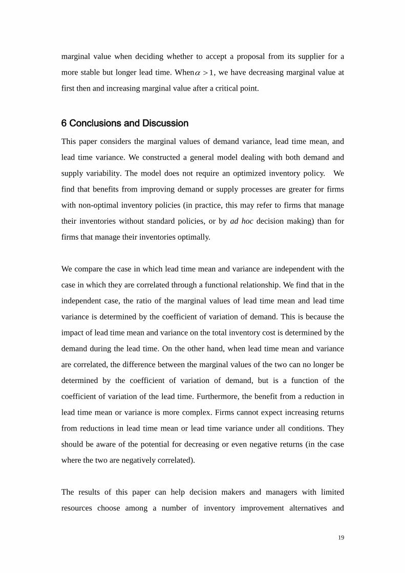
19
marginal value when deciding whether to accept a proposal from its supplier for a
more stable but longer lead time. When 1 , we have decreasing marginal value at
first then and increasing marginal value after a critical point.
6 Conclusions and Discussion
This paper considers the marginal values of demand variance, lead time mean, and
lead time variance. We constructed a general model dealing with both demand and
supply variability. The model does not require an optimized inventory policy. We
find that benefits from improving demand or supply processes are greater for firms
with non-optimal inventory policies (in practice, this may refer to firms that manage
their inventories without standard policies, or by ad hoc decision making) than for
firms that manage their inventories optimally.
We compare the case in which lead time mean and variance are independent with the
case in which they are correlated through a functional relationship. We find that in the
independent case, the ratio of the marginal values of lead time mean and lead time
variance is determined by the coefficient of variation of demand. This is because the
impact of lead time mean and variance on the total inventory cost is determined by the
demand during the lead time. On the other hand, when lead time mean and variance
are correlated, the difference between the marginal values of the two can no longer be
determined by the coefficient of variation of demand, but is a function of the
coefficient of variation of the lead time. Furthermore, the benefit from a reduction in
lead time mean or variance is more complex. Firms cannot expect increasing returns
from reductions in lead time mean or lead time variance under all conditions. They
should be aware of the potential for decreasing or even negative returns (in the case
where the two are negatively correlated).
The results of this paper can help decision makers and managers with limited
resources choose among a number of inventory improvement alternatives and
20
determine where to invest their resources, even when they face poorly managed
inventory or no standard inventory policy. Employing data on the demand or lead
time distributions, the results concerning marginal values provide managers with
guidance about the effects of changing demand variation, lead time mean, and lead
time variation. At the same time, the incentive to change reminds managers of the
importance of inventory management improvement, especially for firms that have
paid little attention to their inventory policies - since they stand to gain even more.
We contend that many assumptions, such as requiring an optimal inventory policy,
may not be essential for modeling purposes. As non-optimal policies are common in
practice (e.g., the cases mentioned by Blackburn, [23]), it may prove useful to relax
the optimality assumptions and to compare the differences. The current paper has
made a step in this direction.
The paper has some limitations that may warrant extensions. For example, we assume
that lead time mean and variance are correlated through a deterministic equation,
whereas in practice firms may be faced with various discrete improvement plans
reflected by a different α and β, in which case our continuous model may not be a
good fit. We plan to test this issue in future research.
References
[1] Lee HL, Padmanabhan V, Whang S. Information distortion in a supply chain: the bullwhip
effect. Management Science 1997; 43(4); 546-559.
[2] Lee HL, So KC, Tang CS. The value of information sharing in a two-level supply chain.
Management Science 2000; 46(5); 626-643.
[3] Fu Y, Piplani R. Supply-side collaboration and its value in supply chains. European Journal of
Operational Research 2004; 152(1); 281-288.
[4] Lim WS. Producer-supplier contracts with incomplete information. Management Science 2001;
47(5); 709-715.
21
[5] Ganeshan, R, Jack, E, Magazine, MJ, Stephens, P. A taxonomic review of supply chain
management research in Quantitative Models for Supply Chain Management, S Tayur, R
Ganeshan, and M Magazine, editors, Kluwer Academic Press 1999; 839-879.
[6] Swaminathan JM, Tayur SR. Models for supply chains in e-business. Management Science
2003; 49(10); 1387-1406.
[7] Flynn BB, Huo B, Zhao X. The impact of supply chain integration on performance: A
contingency and configuration approach. Journal of Operations Management 2010; 28(1); 58-71.
[8] Silver EA. Changing the givens in modelling inventory problems: the example of just-in-time
systems. International Journal of Production Economics 1992; 26(1-3); 347-351.
[9] Smith WI, Lockamy A. Target costing for supply chain management: An economic framework.
Journal of Corporate Accounting & Finance 2000; 12(1); 67-77.
[10] Ryu SW, Lee KK. A stochastic inventory modelof dualsourced supply chain with lead-time
reduction. International Journal of Production Economics 2003; 81–82; 513–524.
[11] Hayya JC, Harrison TP, He XJ. The impact of stochastic lead time reduction on inventory
cost under order crossover. European Journal of Operational Research 2011; 211; 274-281.
[12] Zhang C, Tan GW, Robb DJ, Zheng X. Sharing shipping quantity information in the supply
chain. Omega 2006 ; 34(5); 427-438.
[13] Song JS, Yano CA, Lerssrisutiya P. Contract assembly: dealing with combined supply lead
time and demand quantity uncertainty. Manufacturing & Service Operations Management 2000;
2(3); 287-296.
[14] Qi L, Shen ZM. A supply chain design model with unreliable supply. Naval Research
Logistics 2007; 54 (8); 829-844.
[15] Gerchak Y, Parlar M. Investing in reducing lead-time randomness in continuous-review
inventory models. Engineering Costs and Production Economics 1991; 21; 191-197.
[16] Das C. Effect of lead time on inventory: a static analysis. Operational Research Quarterly
1975; 26(2); 273-282.
[17] Wu J, Zhai X, Huang Z. Incentives for information sharing in duopoly with capacity
constraints. Omega 2008; 36(6); 963-975.
[18] Hosoda T, Disney SM. A delayed demand supply chain: Incentives for upstream players.
Omega 2012; 40(4); 478-487.
22
[19] Bashyam S, Fu MC. Optimization of (s,S) inventory systems with random lead times and a
service level constraint. Management Science 1998; 44(12); 243-256.
[20] Bookbinder JH, Çakanyildirim M. Random lead times and expedited orders in (Q,r) inventory
systems. European Journal of Operational Research 1999; 115; 300-313.
[21] Hayya JC, Christy DP, Pan A. Reducing inventory uncertainty: A reorder point system.
Production and Inventory Management Journal 1987; 28(2); 43-49.
[22] Fisher M, Rajaram K, Raman A. Optimizing inventory replenishment of retail fashion
products. Manufacturing & Service Operations Management 2001; 3(3); 230-241.
[23] Blackburn JD. Limits of time-based competition: strategic sourcing decisions in
make-to-stock manufacturing in Quantitative Approaches to Distribution Logistics and supply
Chain Management, Chapter 3, Klose, Speranza, and Wassenhove , editors, Springer-Verlag 2002.
[24] Garcia CA, Ibeas A, Herrera J, Vilanova R. Inventory control for the supply chain: An
adaptive control approach based on the identification of the lead-time. Omega 2012; 40(3);
314-327.
[25] Chandra C, Grabis J. Inventory management with variable lead-time dependent procurement
cost. Omega 2008; 36; 877 – 887.
[26] Wang P, Hill JA. Recursive behavior of safety stock reduction: The effect of lead-time
uncertainty. Decision Sciences 2006; 37(2); 285-290.
[27] Paknejad MJ, Nasri F, Affisco JF. Lead-time variability reduction in stochastic inventory
models. European Journal of Operational Research 1992; 62(3); 311-322.
[28] Vinson C. The cost of ignoring lead-time unreliability in inventory theory. Decision Sciences
1972; 3(2); 87-105.
[29] Chopra S, Reinhardt G, Dada M. The effect of lead time uncertainty on safety stocks.
Decision Sciences 2004; 35(1); 1-24.
[30] He XJ, Kim JG, Hayya JC. The cost of lead-time variability: The case of the exponential
distribution. International Journal of Production Economics 2005; 97(2); 130-142.
[31] Silver EA, Pyke DF, Peterson R. Inventory management and production planning and
scheduling. John Wiley & Sons, New York, NY, 1998.
[32] Silver EA, Bischak DP. The exact fill rate in a periodic review base stock system under
normally distributed demand. Omega 2011; 39(3); 346-349.
23
[33] Silver EA, Robb DJ. Some insights regarding the optimal reorder period in periodic review
inventory systems. International Journal of Production Economics 2008; 112(1); 354-366.
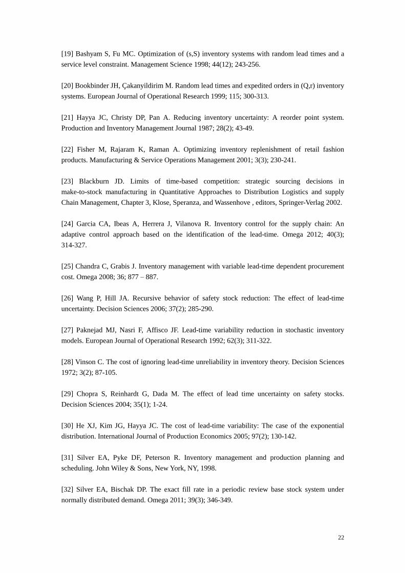
Appendix
Proof of Proposition 1:
0)(4 3
2
2
k
MVD
X
L
D
and 0)(
8
35
3
4
2
k
MVD
X
L
D
;
0)(4 3
4
k
MML
X
D
L
and 0)(
8
35
6
2
2
k
MML
X
D
L
;
0)(4 3
4
2
k
MVL
X
D
L
and 0)(
8
35
6
4
2
k
MVL
X
D
L
.
Since the first and second partial derivatives of MVD, MML and MVL with respect to
2
D , L and 2
L are, respectively, negative and positive, the convex and decreasing
characters of the functions are established. Q.E.D.
Proof of Proposition 2:
Since TC(k) is minimized at k*, 0k
)(TC
*
kk
k and .0
k
)(TC
*
2
2
kk
k As k is only
contained in expression (2), 0k
)(
*
kk
k and .0
k
)(
*
2
2
kk
kFurthermore,
0k
)(
2k
MVD
**
kkX
L
kk
k
and 0
k
)(
2k
MVD
**
2
2
2
2
kkX
L
kk
k
.
Therefore, MVD is minimized at k*. For MML and MVL, the proof is identical. Q.E.D.
Proof of Proposition 3:
Define 22122 2 DLDM . Then for ]2
1,0( , we have
,0)(]4
)12([
3
22222
kMML
X
M
X
DL
L
24
.0)(]8
3)12(
2
)12()22)(12([
5
3
3
2222
3
22222232
2
2
k
MML
X
M
X
MDL
X
MDL
X
DL
L
Similarly, we define 21
2
1
2
/1
2 )(2
1DLDV
and for ),2
1[
,0)(42
))(12
1(
2
1
3
2
22
2
1
2
/1
2
kMVL
X
V
X
DL
L
.0)(]8
3
2
))(12
1(
2
1
4
))(12
1(
2
1
2
))(22
1)(1
2
1(
2
1
[
5
3
3
22
2
1
2
/1
3
22
2
1
2
/1
23
2
1
2
/1
4
2
k
MVL
X
V
X
VDL
X
VDL
X
DL
L
Q.E.D.
Proof of Proposition 4:
(a) Consider the first derivative of MMLE to calculate the critical point for L :
.0)(]4
)2()12([
3
2221222222
kMML
X
DLD
X
DL
L
After simplification, we have
.0)1(8)1(4 4222124424
DDDLDL
If 1 , we have 0
L
MML
for all 0L .
For 1 , define 2212
DL . Then one can view the above as a quadratic
function of with 2
21 2 D , )1(4
4
21
D and discriminant
4422 )1(16)1(64 DD , where 21, are the two real roots of the function.

25
Then, if )1,0( , the function has no positive roots and 0
L
MML
for all 0L .
If 0
or 1 , the function has one positive root * ( *
L accordingly). Then
L
MML
changes sign at that point.
(b) The proof is similar, with the simplified equation:
.0))(14
1(
2))(1
4
1(
1 422/112/124/22/12
DDDLDL
Then we can define 2/112/12 )(' DL and obtain the required result. Q.E.D.