Embed Size (px)
Citation preview
Vera Rita Costa Salgado
Licenciatura em Ciências da Engenharia Biomédica
Analysis of functional Magnetic Resonance datafor neurosurgical planning: subject specific
resting state analysis as a complement to taskbased analysis.
Dissertação para obtenção do Grau de Mestre em
Engenharia Biomédica
Orientador: Alexandre Andrade, Doutor,Instituto de Biofísica e Engenharia Biomédica, Faculdadede Ciências da Universidade de Lisboa
Júri
Presidente: Doutora Carla Maria Quintão PereiraArguente: Doutor Ricardo Nuno Pereira Verga e Afonso Vigário
Vogal: Doutor Alexandre da Rocha Freire de Andrade
September, 2016

Analysis of functional Magnetic Resonance data for neurosurgical planning:subject specific resting state analysis as a complement to task based analysis.
Copyright © Vera Rita Costa Salgado, Faculdade de Ciências e Tecnologia, Universidade
NOVA de Lisboa.
A Faculdade de Ciências e Tecnologia e a Universidade NOVA de Lisboa têm o direito,
perpétuo e sem limites geográficos, de arquivar e publicar esta dissertação através de
exemplares impressos reproduzidos em papel ou de forma digital, ou por qualquer outro
meio conhecido ou que venha a ser inventado, e de a divulgar através de repositórios
científicos e de admitir a sua cópia e distribuição com objetivos educacionais ou de
investigação, não comerciais, desde que seja dado crédito ao autor e editor.
Este documento foi gerado utilizando o processador (pdf)LATEX, com base no template “unlthesis” [1] desenvolvido no Dep. Informática da FCT-NOVA[2]. [1] https://github.com/joaomlourenco/unlthesis [2] http://www.di.fct.unl.pt


Aos meus pais, irmão e avó.


Acknowledgements
First of all, I would like to thank the Institute of Biophysics and Biomedical Engineering
(IBEB), where this dissertation was conducted, for all the support provided during this
time.
I want to express my deepest gratitude to my supervisor, Alexandre Andrade. His
guidance, support and availability were crucial for the success of this project. I am
sincerely thankful for all the knowledge and experience achieved working with him.
I would also like to thank Dr. Martin Lauterbach, for the attentiveness and valuable
contribution to this study.
To my parents, Cristina and José, I would like to say how grateful I am for all the
emotional support and encouragement, not only in the last few months, but during
my whole life. Thank you for the values that you transmitted, they are now far more
treasured than ever. With the same gratitude I also would like to mention my brother,
Francisco, for being supportive in his funny, but lovely way, and to my grandmother for
all the knowledge and for being a role model my entire life.
To all people whom I shared my workspace with, I am thankful for all the assistance,
dedication and companionship. Without you my lunch time would be certainly shorter
but I wouldn’t have so many memorable moments to share. I thank each and every one
of you for helping me in different occasions, giving me the support I needed and for
making this experience a remarkable one.
I also should not forget those who joined me in my academic journey. Your compan-
ionship will not be forgotten.
Finally, I would like to thank my hometown friends, the ones that I grew up with.
Thank you for understanding my absence during the last 5 years. I know you are, as
you always have been, rooting for my success.
The limited space of this acknowledgment section does not allow me to thank prop-
erly all the people who helped me achieve this new stage of my academic path. I will
always cherish your friendship and think of you with fond memories. To all such people
in my life, I am sincerely grateful.
vii


Abstract
Brain and other central nervous system tumors are the 17th most common cancer
type in Europe, being associated with high mortality rate. Neurosurgery has been
the ultimate solution for the treatment of brain tumors. Integration of preoperative
brain mapping in the process is highly recommended in order to preserve fundamental
areas of the brain, especially those believed to be connected to language and movement.
Recently, there has been a growing interest in presurgical planning resorting to resting-
state functional magnetic resonance imaging (fMRI).
The aim of this thesis is to explore strategies to process data of resting-state fMRI
in order to better understand its connection to task brain networks, and to assess their
application to the protocols currently used within clinical institutions that are partners
of the host scientific institution in an ongoing project. A total of 8 subjects were re-
cruited to participate in this study, all of them previously referred for surgical tumor
resection. An optimal strategy for pre-processing was devised and tested. Task data was
processed using the General Linear Model, while rest data was processed through Inde-
pendent Component Analysis. The processed data were then correlated via similarity
coefficients.
The results of similarity tests show a limited coincidence between resting-state net-
works and the activation task areas. Further studies will be required in order to improve
these results.
Keywords: Brain tumors, fMRI, General Linear Model, Independent Component Anal-
ysis, resting-state
ix


Resumo
Os tumores cerebrais, juntamente com outros tumores do sistema nervoso central são o
17º tipo de cancro mais comum na Europa, estando associados a uma elevada taxa de
mortalidade. A neurocirurgia tem sido uma das soluções para o seu tratamento. Neste
âmbito, a integração do mapeamento cerebral pré-cirúrgico no processo é altamente
recomendada a fim de preservar áreas fundamentais do cérebro, nomeadamente as que
estão relacionadas com a linguagem e com o movimento. Recentemente, tem havido um
crescente interesse no planeamento pré-cirúrgico com recurso à imagem de ressonância
magnética funcional em repouso.
O objetivo desta tese é explorar estratégias para processar dados de ressonância
magnética funcional em repouso, com o intuito de compreender a sua relação com re-
des cerebrais provenientes de paradigmas de tarefa, e explorar a aplicabilidade dessas
estratégias nos protocolos actualemnte usados nas instituições clínicas associadas à ins-
tituição de acolheminto, no contexto de um projecto em curso. Um total de 8 indivíduos
foram recrutados para participar neste estudo, todos eles previamente referenciados
para resseção cirúrgica do tumor. Foi concebida e testada uma estratégia otimizada para
o pré-processamento. Os dados de tarefa foram processados utilizando o Modelo Linear
Geral, ao passo que os dados de repouso foram processados através da análise de com-
ponentes independentes. Os dados processados foram posteriormente correlacionados
através de coeficientes de similaridade.
Os resultados dos testes de similaridade mostram uma coincidência limitada entre
as redes de repouso e as áreas de ativação provenientes de paradigmas de tarefa. Serão
necessários mais estudos de forma a melhorar estes resultados.
Palavras-chave: Análise em componentes independentes, Imagem por Ressonância
Magnética Funcional, Modelo Linear Geral, Repouso, Tumores cerbrais.
xi

xii

Contents
List of Figures xv
List of Tables xvii
Acronyms xix
1 Introduction 1
1.1 Objectives . . . . . . . . . . . . . . . . . . . . . . . . . . . . . . . . . . . 2
1.2 Dissertation overview . . . . . . . . . . . . . . . . . . . . . . . . . . . . . 3
2 Background 5
2.1 Brain Tumors - Basic Concepts . . . . . . . . . . . . . . . . . . . . . . . . 5
2.1.1 Eloquent Areas . . . . . . . . . . . . . . . . . . . . . . . . . . . . 6
2.2 Surgical Planning . . . . . . . . . . . . . . . . . . . . . . . . . . . . . . . 7
2.2.1 Brain Imaging Techniques . . . . . . . . . . . . . . . . . . . . . . 7
2.2.2 Magnetic Resonance Imaging . . . . . . . . . . . . . . . . . . . . 9
2.2.3 Resting State functional Magnetic Resonance Imaging . . . . . . 11
2.2.4 fMRI processing . . . . . . . . . . . . . . . . . . . . . . . . . . . . 14
3 Materials and methods 21
3.1 Participants and Image acquisition . . . . . . . . . . . . . . . . . . . . . 21
3.2 Preprocessing . . . . . . . . . . . . . . . . . . . . . . . . . . . . . . . . . 23
3.3 Processing . . . . . . . . . . . . . . . . . . . . . . . . . . . . . . . . . . . 28
3.3.1 Task data - Statistical Analysis . . . . . . . . . . . . . . . . . . . . 28
3.3.2 Rest data processing . . . . . . . . . . . . . . . . . . . . . . . . . 32
3.4 Comparison of Task Networks and Resting State Networks . . . . . . . 33
4 Results 37
4.1 Important results from preprocessing . . . . . . . . . . . . . . . . . . . . 37
xiii
CONTENTS
4.1.1 Scrubbing . . . . . . . . . . . . . . . . . . . . . . . . . . . . . . . 37
4.1.2 Normalization . . . . . . . . . . . . . . . . . . . . . . . . . . . . . 38
4.1.3 Removal of nuisance signals . . . . . . . . . . . . . . . . . . . . . 40
4.2 Intra-Subject Analysis . . . . . . . . . . . . . . . . . . . . . . . . . . . . . 41
4.2.1 Motor Paradigms . . . . . . . . . . . . . . . . . . . . . . . . . . . 41
4.2.2 Language . . . . . . . . . . . . . . . . . . . . . . . . . . . . . . . . 56
4.3 Intra-Task Analysis . . . . . . . . . . . . . . . . . . . . . . . . . . . . . . 64
4.4 Results Overview . . . . . . . . . . . . . . . . . . . . . . . . . . . . . . . 72
5 Discussion 73
6 Conclusion 77
Bibliography 79
xiv

List of Figures
2.1 Classic anatomic sites for functional brain areas . . . . . . . . . . . . . . . . 13
2.2 Resting-State networks . . . . . . . . . . . . . . . . . . . . . . . . . . . . . . 14
3.1 DPARSFA layout . . . . . . . . . . . . . . . . . . . . . . . . . . . . . . . . . . 24
3.2 DPARSFA options . . . . . . . . . . . . . . . . . . . . . . . . . . . . . . . . . 27
3.3 SPM layout . . . . . . . . . . . . . . . . . . . . . . . . . . . . . . . . . . . . . 29
3.4 fMRI model specification . . . . . . . . . . . . . . . . . . . . . . . . . . . . . 30
3.5 GIFT layout . . . . . . . . . . . . . . . . . . . . . . . . . . . . . . . . . . . . 33
3.6 GIFT options . . . . . . . . . . . . . . . . . . . . . . . . . . . . . . . . . . . . 34
3.7 The overall scheme . . . . . . . . . . . . . . . . . . . . . . . . . . . . . . . . 36
4.1 Difference between normalize and not normalize images . . . . . . . . . . . 39
4.2 Effect of nuisance signals removal . . . . . . . . . . . . . . . . . . . . . . . . 40
4.3 Mouth activation map for Sub003 . . . . . . . . . . . . . . . . . . . . . . . . 42
4.4 SPM environment . . . . . . . . . . . . . . . . . . . . . . . . . . . . . . . . . 44
4.5 Rest and task correlation map . . . . . . . . . . . . . . . . . . . . . . . . . . 45
4.6 Independent Component of Sub003 rest network . . . . . . . . . . . . . . . 46
4.7 Hands activation maps for Sub003 . . . . . . . . . . . . . . . . . . . . . . . 49
4.8 Rest activation maps for Sub003 . . . . . . . . . . . . . . . . . . . . . . . . . 50
4.9 Feet activation maps for Sub003 . . . . . . . . . . . . . . . . . . . . . . . . . 52
4.10 Rest activation maps for Sub003 . . . . . . . . . . . . . . . . . . . . . . . . . 53
4.11 Syntactic Decisions activation maps for Sub003 . . . . . . . . . . . . . . . . 57
4.12 Independent Component of Sub003 rest network that is more similar with
the syntactic decision activation map . . . . . . . . . . . . . . . . . . . . . . 58
4.13 Independent Component of Sub003 rest network that is more similar with
the verb generation activation map . . . . . . . . . . . . . . . . . . . . . . . 60
4.14 Independent Component of Sub003 rest network that is more similar with
the verb generation activation map . . . . . . . . . . . . . . . . . . . . . . . 61
xv

List of Tables
2.1 Brain tumor classification . . . . . . . . . . . . . . . . . . . . . . . . . . . . 6
3.1 Demographic features of the study population . . . . . . . . . . . . . . . . 22
4.1 Scrubbing Results . . . . . . . . . . . . . . . . . . . . . . . . . . . . . . . . . 38
4.2 Similarity results for rest activation maps and mouth paradigm activation
maps for Sub003 . . . . . . . . . . . . . . . . . . . . . . . . . . . . . . . . . . 47
4.3 Similarity results for rest activation maps and mouth paradigm activation
maps for Sub003, with nuisance signals removal . . . . . . . . . . . . . . . 48
4.4 Similarity results for rest activation maps and hands paradigm activation
maps for Sub003 . . . . . . . . . . . . . . . . . . . . . . . . . . . . . . . . . . 51
4.5 Similarity results for rest activation maps and feet paradigm activation maps
for Sub003 . . . . . . . . . . . . . . . . . . . . . . . . . . . . . . . . . . . . . 54
4.6 Similarity test results for rest activation maps and with the result of the
superposition of the 3 motor tasks for Sub003 . . . . . . . . . . . . . . . . . 55
4.7 Similarity results for rest activation maps and syntactic decision paradigm
activation maps for Sub003 . . . . . . . . . . . . . . . . . . . . . . . . . . . . 59
4.8 Similarity test results for rest activation maps and verb generation paradigm
activation maps for Sub003 . . . . . . . . . . . . . . . . . . . . . . . . . . . . 62
4.9 Similarity test results for rest activation maps and with the result of the
superposition of the 3 motor tasks for Sub003 . . . . . . . . . . . . . . . . . 63
4.10 Similarity test results for rest activation maps and hand activation maps for
Sub001 . . . . . . . . . . . . . . . . . . . . . . . . . . . . . . . . . . . . . . . 64
4.11 Similarity test results for rest activation maps and hand activation maps for
Sub002 . . . . . . . . . . . . . . . . . . . . . . . . . . . . . . . . . . . . . . . 65
4.12 Similarity test results for rest activation maps and hand activation maps for
Sub001 . . . . . . . . . . . . . . . . . . . . . . . . . . . . . . . . . . . . . . . 66
xvii

List of Tables
4.13 Similarity test results for rest activation maps and hand activation maps for
Sub004 . . . . . . . . . . . . . . . . . . . . . . . . . . . . . . . . . . . . . . . 67
4.14 Similarity test results for rest activation maps and hand activation maps for
Sub005 . . . . . . . . . . . . . . . . . . . . . . . . . . . . . . . . . . . . . . . 68
4.15 Similarity test results for rest activation maps and hand activation maps for
Sub006 . . . . . . . . . . . . . . . . . . . . . . . . . . . . . . . . . . . . . . . 69
4.16 Similarity test results for rest activation maps and hand activation maps for
Sub007 . . . . . . . . . . . . . . . . . . . . . . . . . . . . . . . . . . . . . . . 70
4.17 Similarity test results for rest activation maps and hand activation maps for
Sub008 . . . . . . . . . . . . . . . . . . . . . . . . . . . . . . . . . . . . . . . 71
xviii

Acronyms
BET brain extraction tool.
BOLD blood oxygenation level dependent.
CNS central nervous system.
CSF cerebrospinal fluid.
DICOM Digital Imaging and Communications in Medicine.
DMN default-mode network.
DNA deoxyribonucleic acid.
DPABI Data Processing and Analysis for Brain Imaging.
DPARSFA Data Processing Assistant for Resting-State fMRI- advanced edition.
DSC Dice similarity coefficient.
ECS electrical cortical stimulation.
EEG electroencephalography.
FD frame-wise displacements.
fMRI functional magnetic resonance imaging.
FWE familywise error.
FWHM full width at half maximum.
GIFT Group independent component analysis (ICA) of functional magnetic resonance
imaging (fMRI) toolbox.
xix

ACRONYMS
GLM General Linear Model.
hrf hemodynamic response function.
IC independent component.
ICA independent component analysis.
MEG magnetoencephalography.
MNI Monreal Neurological Institute.
MRI magnetic resonance imaging.
NIfTI Neuroimaging Informatics Technology Initiative.
PC principal components.
PCA principal component analysis.
PET positron emission tomography.
ReML restricted maximum likelihood.
REST Resting-State fMRI Data Analysis Toolkit.
Rf Radiofrequency.
rs-fMRI resting state functional magnetic resonance imaging.
RSN resting state networks.
SMN sensorimotor network.
SN salience network.
SPM Statistical Parametric Mapping.
TE echo time.
TR repetition time.
WM white matter.
xx

Chapter
1Introduction
Tumors of the central nervous system are associated with a high incidence and mortality
rate. In 2012, brain and other central nervous system cancer was reported to be the 17th
most common cancer type and the 12th most common cause of cancer death worldwide.
Neurosurgery has been the ultimate solution for the treatment of these pathologies, with
really satisfactory outcomes [1]. Nevertheless, in those circumstances, integration of
preoperative brain mapping in the process is highly recommended in order to preserve
fundamental areas of the brain, especially those believed to be connected to language
and movement, denominated eloquent areas, and reduce post-operative deficits [2]
[3]. In this scope, the search for an accurate knowledge about the structure and func-
tionality of the brain has been one of the most important challenges for pre-planning
neurosurgery.
In the early ages of neurosurgery only standard structural and functional maps were
used to help neurosurgical planning. However, according to several scientific studies,
the association between anatomical and functional areas shows high inter- subject vari-
ability [4]. Functional connectivity using fMRI, possibly complemented with other non-
invasive imaging methods like electric source imaging (EEG), magnetoencephalography
(MEG), positron emission tomography (PET), single photon emission computed tomog-
raphy (SPECT) and functional magnetic resonance imaging (fMRI) has been adopted
in order to trace network connections that are subject-specific and therefore to provide
additional information that is useful for presurgical mapping [5] [2]. More specifically,
1

CHAPTER 1. INTRODUCTION
fMRI, as an innocuous approach, has proven to be a promising technique to acquire the
activation sites of the human brain involved in the eloquent functions, through assess-
ment of changings in blood oxygenation level dependence (BOLD) [3]. Typically, fMRI
appraises small hemodynamic fluctuations induced by stimulus or by task performance
[3] [6].
Nonetheless, recent developments led to the belief that there is a temporal and
functional correlation among separated brain regions, responsible for behavioral and
cognitive functions control, even in rest conditions. In addition, there are small changes
in BOLD signal during rest that confirm an incessant interaction between brain net-
works, thus leading to Resting-State Network [2] [3] [7]. Despite the increasing interest
in this new approach, there is still a long way ahead until resting-state fMRI is com-
pletely accepted and applied inside the clinical realm [8].
1.1 Objectives
The aim of this thesis is to explore strategies for resting-state fMRI data processing in
order to better understand its relationship with brain networks from task paradigms and
its contribution in improving diagnosis and pre-surgical planning. As a result, subjects
unable to perform tasks, such as asleep or anesthetized patients, could benefit from this
diagnostic technique, since it does not require the performance of any task. For this
purpose, it is intended to test and optimize a preprocessing protocol, followed by the
adaptation of some processing protocols used in the literature, devised for the task and
rest data individually. Finally, it is intended to employ the results from these procedures
in similarity analysis, aiming to realize the resemblance between brain activation in task
performing and at rest, in order to test the reliability of resting state data analysis to
complement the classic task approach in pre-surgical planning.
The work carried out within this thesis was hosted by the Institute of Biophysics
and Biomedical Engineering of the Faculty of Sciences of the University of Lisbon, in
the context of an ongoing collaboration with Sociedade Portuguesa de Ressonância
Magnética/Hospital da Cruz Vermelha and Centro Hospitalar de Lisboa Norte/Hospital
de Santa Maria.
2

1.2. DISSERTATION OVERVIEW
1.2 Dissertation overview
This section aims to present a brief description of topics covered in each chapter in
order to provide an enlightened reading.
Chapter 2. Background reviews the background literature related to the work de-
veloped in this dissertation. In particular, it provides some basic concepts about brain
tumours, such as the brain mapping methodologies commonly used for surgical plan-
ning, which includes a description of functional magnetic resonance imaging ant its
newest approach, resting state fMRI.
Chapter 3. Materials and methods details how the current study was conducted,
undergoing a brief exposition of the software and methodology implemented. It also
presents a brief description of the participants and the image acquisition protocol, fol-
lowed by the detailed information about the methods and software used in the prepro-
cessing and processing stages Finally, it is explained how the task based and resting
state maps were superimposed such as its correlation calculation.
Chapter 4. Results intends to report the most relevant results obtained in pre-
processing and processing stages, followed by the presentation of statistical and simi-
larity analysis results.
Chapter 5. Discussion presents the analysis and discussion of the study results, as
some limitations and suggestions for improvement.
Chapter 6. Conclusion provides the overall conclusions and suggestions for future
work.
3


Chapter
2Background
2.1 Brain Tumors - Basic Concepts
The human brain composes the central nervous system (CNS) along with the spinal
cord and meninges. Taken together, they are responsible for controlling the majority
of the bodily functions [9]. As with all other parts of the body, the CNS comprises nu-
merous cells some of whose functions are managed by the deoxyribonucleic acid (DNA)
, which is contained in their nuclei. When DNA carries a disability these functions
may be compromised. More specifically, mutation of DNA can affect the production,
growth and division cycle of cells, leading to an abnormal mass accumulation which
compresses and damages the surrounding brain areas, commonly named as brain tumor
or intracranial neoplasm [10].
Brain tumors are highly variable in shape, size and localization.They can be catego-
rized as primary or metastatic. The first group refers to an abnormal mass that arises
originally from the brain, whereas the second one refers to tumors that begin outside
the CNS and then spread to the brain, such as metastasis from breast, lung and kidney
cancer [11].
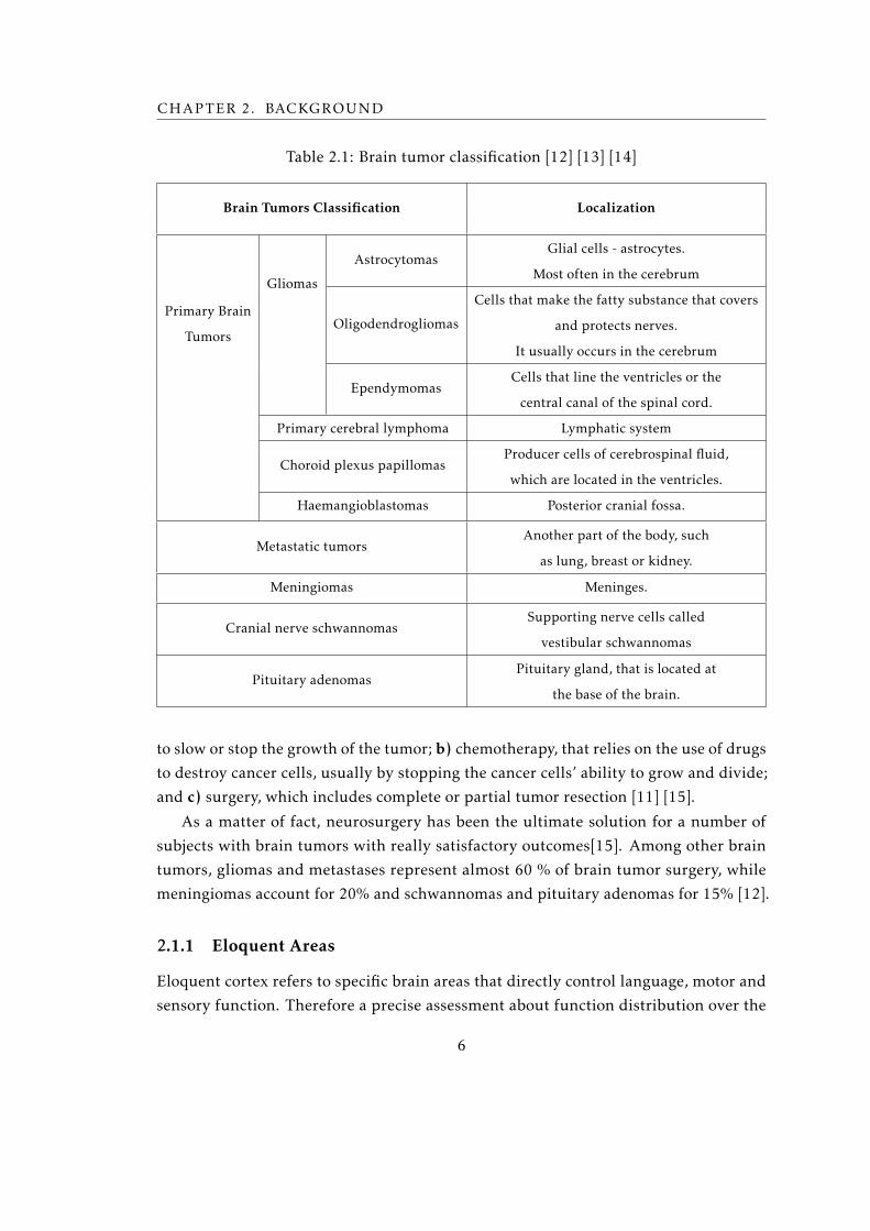
Brain tumors have their designations by the location in which they begin. Some of
these are listed in table 2.1.
Treatment options vary with tumor location and severity. The most widely used al-
ternatives are: a) radiation therapies, that use high energy beams of photons or particles
5
CHAPTER 2. BACKGROUND
Table 2.1: Brain tumor classification [12] [13] [14]
Brain Tumors Classification Localization
Primary Brain
Tumors
Gliomas
AstrocytomasGlial cells - astrocytes.
Most often in the cerebrum
Oligodendrogliomas
Cells that make the fatty substance that covers
and protects nerves.
It usually occurs in the cerebrum
EpendymomasCells that line the ventricles or the
central canal of the spinal cord.
Primary cerebral lymphoma Lymphatic system
Choroid plexus papillomasProducer cells of cerebrospinal fluid,
which are located in the ventricles.
Haemangioblastomas Posterior cranial fossa.
Metastatic tumorsAnother part of the body, such
as lung, breast or kidney.
Meningiomas Meninges.
Cranial nerve schwannomasSupporting nerve cells called
vestibular schwannomas
Pituitary adenomasPituitary gland, that is located at
the base of the brain.
to slow or stop the growth of the tumor; b) chemotherapy, that relies on the use of drugs
to destroy cancer cells, usually by stopping the cancer cells’ ability to grow and divide;
and c) surgery, which includes complete or partial tumor resection [11] [15].
As a matter of fact, neurosurgery has been the ultimate solution for a number of
subjects with brain tumors with really satisfactory outcomes[15]. Among other brain
tumors, gliomas and metastases represent almost 60 % of brain tumor surgery, while
meningiomas account for 20% and schwannomas and pituitary adenomas for 15% [12].
2.1.1 Eloquent Areas
Eloquent cortex refers to specific brain areas that directly control language, motor and
sensory function. Therefore a precise assessment about function distribution over the
6

2.2. SURGICAL PLANNING
human brain is necessary for the presurgical planification. Damage to these areas gen-
erally leads to major neurological deficits. Brain areas responsible for motor function
are mostly located in the precentral gyrus just anterior to the central sulcus. However,
there are several other areas that are likewise relevant to body motion. Premotor and
supplementary motor area include brain regions responsible for planning and control-
ling movement. Both of those areas are located in the mesial and lateral side of superior
frontal gyrus, forward to precentral sulcus. The communication of those different areas
throughout the corticospinal fiber tract is responsible for coordination and synchronic-
ity of movements. [16].
Sensorial information follows the inverse pathway of motor function and it is mainly
directed to the primary somatosensitive area, located in the postcentral gyrus, posterior
to the central sulcus [17] [16].
Broca’s area, believed to be one of the areas responsible for speech production, is
anatomically located in the inferior frontal gyrus and it is composed by two areas: the
pars triangularis and the pars opercularis. The function of Broca’s area is to command
the muscles so that they produce meaningful sounds. Broca’s area is connected to
Wernicke’s area through a white-matter fiber tract called arcuate fasciculus. Wernicke’s
area is one of the areas responsible for language understanding. It’s placed on the
back portion of temporal lobe of the dominant hemisphere, that generally is the left
hemisphere [17].
2.2 Surgical Planning
The challenge of brain lesions’ surgical resection is balancing the aim of maximizing
resection with the requirement to preserve functionally-relevant brain areas, especially
those believed to be connected to language and movement, denominated eloquent ar-
eas[16]. In this scope, accurate localization of those areas is essential for presurgical
planning, as it helps optimize resection and decrease postoperative deficits [18] [6] [3].
2.2.1 Brain Imaging Techniques
In the early ages of neurosurgery only standard structural and functional maps were
used to help neurosurgical planning. Nevertheless, according to several scientific stud-
ies, anatomical and functional areas have high inter-subject variability owing, not only,
to individual characteristics of cortical organization, but also to functional reorganiza-
tion in response to the individual’s brain pathology [4] [19]. This inconstancy among
7

CHAPTER 2. BACKGROUND
subjects led to a growing concern to develop new imaging techniques capable of creating
individual brain maps.
The first subject specific’s functional mapping procedure was an extremely invasive
technique, called Intracarotid Amobarbital procedure or Wada Test. During this intra-
operative method, an anesthetic medication is injected into the right or left internal
carotid artery putting that hemisphere to sleep and incapable to communicate with the
opposite side [18]. The main goal of this procedure was to determine which side of the
brain controls language function and how significant each hemisphere is in regard to
memory function [20].
The Wada Test has been replaced or complemented by electrical cortical stimulation
(ECS), another invasive procedure that resorts on stimulation of the cerebral cortex’s
surface while the patient is awake and performing motor, language or cognitive con-
trolled tasks. This approach can only be used in intra-operatively stage and as it relies
on the use of anesthetics it may produce unsatisfying outcomes [6] [20].
Regardless of whether the Wada Test or ECS are considered the gold standard pro-
cedures for mapping brain function, both require an awake and cooperative subject.
Their invasive nature led to the need for non-invasive approaches. With the advent of
high resolution non-invasive neuroimaging, there has been improved ability to map
the structure of the brain, as well as its connections. In this scope, techniques such as
fMRI, electroencephalography (EEG), magnetoencephalography (MEG) and positron
emission tomography (PET) have been adopted in order to trace network connections
that are subject-specific and therefore to provide profitable information for pre-surgical
planning assessment [5] [2].
In a brief description, PET is based on the detection and imaging of positron-
emitting radionuclides that were previously administrated to the patient. PET images
demonstrate indirectly functional courses involved in cerebral metabolism. Like other
techniques, such as computed tomography or magnetic resonance imaging (MRI), PET
relies on reconstruction tecquniques to obtain tomographic images. In order to acquire
better anatomic localization of the regions of interest PET images can be overlaid with
anatomic images such as MRI or computed tomography [21].
As for the EEG, it is a direct measure of brain function which records the electrical
activity of the brain resorting to electrodes that are placed on the subject’s scalp. The
time-series of scalp potential maps represent the differences in electric potential of
distinct brain areas [2] [22].
Lastly, MEG measures the brain’s neuronal activity recording its magnetic fields.
8

2.2. SURGICAL PLANNING
These magnetic fields are generated by neuronal electrical currents. The spatial dis-
tributions of the magnetic fields are analyzed in order to map brain regions involved
in specific functions. Since the magnetic field measured by MEG is produced directly
by electrical neuronal activity, it is possible to detect signals from the brain on a sub-
millisecond time scale [23].
Although all brain mapping techniques should present identical outcomes, inter-
modal variations exist.
2.2.2 Magnetic Resonance Imaging
MRI is an imaging technique that relies on protons and their inherent magnetism to
generate an image. As the human body is composed mainly of water, MRI takes ad-
vantage of the great abundance in hydrogen nucleus (¹H) by manipulating them with
Radiofrequency (Rf) energy in the presence of a strong magnetic field [24].
The hydrogen atom consists of an orbiting electron and a single positively charged
proton (nucleus) which spins around its axis, creating a magnetic moment along the
direction of spins’ axis. The sum of all the magnetic fields of each spin is called net
magnetization. In the absence of an external magnetic field, the nuclei of hydrogen
atoms in a sample are randomly distributed and therefore the sum of all the results in a
null net magnetization. On the other hand, when exposed to a strong static magnetic
field B0, the nuclei will align parallel or anti-parallel to the field. As it requires less
energy, the majority of the spins allign parallely with field B0 creating a magnetization
in that direction. The nuclei precess with an angular frequency determined by the
Larmor frequency ω0. The relation between Larmor frequency and the main magnetic
field strength is displayed in the equation 2.1, where ψ represents the gyromagnetic
ratio. Nevertheless, not all spins rotate in the same phase, therefore the sum of all the
spins’ transverse magnetizations is null.
ω0 = ψ ·B0 (2.1)
The phase equilibrium can be disturbed through a short oscilating magnetic field
(i.e. radiofrequency pulse). Only protons that precess with the same frequency (Larmor
frequency) as the electromagnetic Rf pulse will absorb energy, aligning their phases and
thereby generating a component of the magnetization over the transversal plane (or xy
plane). After the radiofrequency pulse is removed the system returns to equilibrium,
in the process called dephasing, and there is recovery of the longitudinal component
(z-direction) with an emission of electromagnetic energy.
9

CHAPTER 2. BACKGROUND
Longitudinal relaxation corresponds to exponential recovery in longitudinal mag-
netization. It is characterized by the energy exchange between the spins and the sur-
rounding environment. The recovery rate is a constant tissue-specific time generally
called T1. On the other hand transversal relaxation is result of a progressive dephasing
of nuclei following the RF pulse caused by a spin-spin interaction. This inter-dipole
interaction time is an exponential decay in transversal magnetization and is designated
by T2. The MRI ability to create anatomic images is due to the tissue-specific relaxation
times, which enables the differentiation between different tissues.
In actual MRI procedures, the transversal relaxation time is shorter than T2. The in-
consistency results from the inhomogeneities in the main magnetic field. This observed
time, called T2∗, has an essential role on functional Magnetic Resonance Imaging.
2.2.2.1 Functional Magnetic Resonance Imaging
In the last 25 years, the neuroimaging world had suffered several great updates and
innovations. The discovery that MRI could be sensitive to brain activity, besides its
anatomy, was probably the most remarkable one [25].
In regular brain imaging techniques the main goal is to distinguish different tissue
types. Nonetheless, in functional brain imaging the purpose is to assess signal fluctua-
tions over time. fMRI is one functional neuroimaging technique used to measure brain
activity [26].
When a specific brain region increases its activity due to a task or a stimulation,
the initial amount of oxygenated haemoglobin in the nearest blood vessels decreases,
enhancing the deoxygenated haemoglobin. Seconds passed, there is a demanding need
for additional oxygen and thus the blood flow increases, providing a great amount of
oxygenated haemoglobin. fMRI is sensitive to this expansive rebound and the relative
decrease in deoxyhemoglobin concentration, as it introduces a low increment in T 2∗
weighted signal. This phenomenon is called blood oxygenation level dependent (BOLD).
The basic foundation of fMRI is the fundamental difference in the paramagnetic
properties of deoxygenated and oxygenated haemoglobin. The hemoglobin molecule
has magnetic properties that differ whether it is bound to oxygen or not. The oxygenated
hemoglobin (Hb) has no unpaired electron and no magnetic moment (diamagnetic),
therefore it is not magnetically distinct from other tissues. In contrast deoxyhemoglobin
(dHb) has an unpaired electron and magnetic moment (paramagnetic) and thus deoxy-
genated blood differs in its magnetic properties from surrounding tissues [27].
fMRI has had a growing impact in neuroimaging. Since it is a non-invasive and an
10

2.2. SURGICAL PLANNING
ionizing radiation-free technique, fMRI can assess brain function safely. Besides, due to
its good spatial resolution, fMRI has been broadly used in clinical settings. Alongside
the pre-surgical planning, the use of this functional imaging method has played a key
role in functional evaluation in brain tumor management [28], in the study of Parkin-
son’s disease [29], as well as in early detection of Alzheimer’s disease [30], and also in
investigations of psychiatric disorders such as schizophrenia and severe depression [28].
More specifically, in pre-surgical context, fMRI demonstrates great precision in defining
which hemisphere is language dominant, helping to decrease post-operative deficits,
likewise reducing surgical time and improving the decision of the areas to recess.
Recent studies on spontaneous modulations in BOLD signal revealed the repro-
ducibility of traditional fMRI in the absence of stimuli. These advances mean a new
range of applications and prospects of fMRI and this topic will be explored in the next
section.
2.2.3 Resting State functional Magnetic Resonance Imaging
The idea that human’s brain is not idle in periods of resting has been explored since the
IX century [31]. Nevertheless, it was only in the auspicious years for technological de-
velopments that followed the Second World War, when Seymour Kety and Carl Schmidt
first measured whole-brain metabolism and blood flow [32]. Seymour and Schmidt real-
ized that in rest conditions the brain consumes 20% of the body’s energy, 10 times higher
the expected value for only 2% of the body weight. Furthermore, in task performance,
metabolic consumption only increases 5% [32]. This assumption makes clear the evi-
dence of an intrinsic activity which expends the majority of the energy. Years later, the
appearance of imaging techniques such as PET and fMRI brought new developments
in the history of resting-state oscillations. Initially, slow spontaneous fluctuations in
the BOLD-fMRI signal (typically < 0.1 Hz) were considered noise [33]. These artifacts,
or so they thought, would be a result of non-neuronal sources like head motion [34].
Then, in 1995, Biswal and his colleagues were the first to demonstrate the functional
implication of these fluctuations [35]. Biswal, trying to know what was the transfer func-
tion of the sensorimotor cortex, filtered out the respiration signal. The results showed
that neither the respiration nor cardiac signal were the foremost contributors to the
artifacts. In fact, they found that the main sources were lower-frequency signals. In
an attempt to know what sources could provide a signal with that range of frequencies,
they correlated a resting state time-series of a voxel from the sensorimotor cortex with
the resting state time-series of every voxel in the brain. The results showed that the
11
CHAPTER 2. BACKGROUND
strongest correlations were between the left and the right sensorimotor cortices [35].
Later studies confirmed the existence of synchronous fluctuations between other func-
tional networks, like the primary visual network, auditory network and higher order
cognitive networks [35] [36]. Biswal, in addition, showed that resting-state and task-
based activation maps are notably similar [35]. These low frequency BOLD fluctuations
observed while in resting show temporal correlations between anatomical distinct areas
of the brain. These patterns have been designated "intrinsic connectivity networks" or
"resting state networks".
Since initial contributions of Biswal up to the present day, the study of resting-
state networks has shown a huge potential for the diagnosis of several pathologies like
Alzheimer’s, miultiple sclerosis, autism, Tourette syndrome among others [8].
Although the true origin of these resting state BOLD signal oscillations (∼ 0.01 −0.1Hz) is not fully understood yet, it is proven that they are intrinsically generated by
the grey matter and are not consequence of external stimulation.
2.2.3.1 Resting State Networks
The discovery of brain’s resting state networks was accidental. Scans of resting-state
brain started to be included in the task-paradigm studies as a baseline for comparison.
However, investigators noticed that some brain regions were more active in resting
conditions than in controlled task .
The first resting state network to be discovered was default-mode network (DMN).
The default mode network, is a group of brain regions that shows higher levels of activity
when the subject is not involved in any mental exercise. This network is responsible
for memory consolidation, monitoring the environment, keeping awareness even when
resting and other ongoing intrinsic thoughts. Anatomically, the regions involved on
this network are generally the medial prefrontal cortex, posterior cingulate cortex, and
the inferior parietal lobule. Other regions as the lateral temporal cortex, hippocampal
formation, and the precuneus are also described in literature as being included in DMN
[37]. For an enlightened interpretation consult figure 2.1.
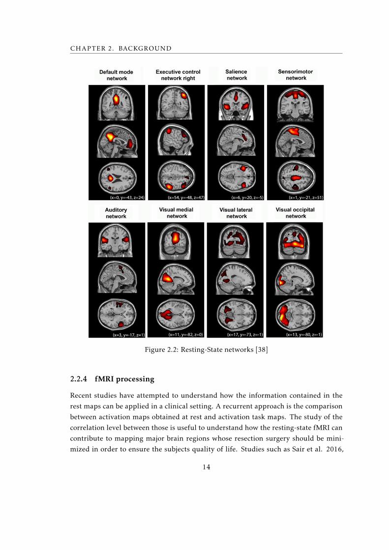
Several other resting state networks (RSN) have been studied and described in liter-
ature. Although there is no concordance on names or localizations, there are 4 major
resting-state networks in addition to DMN: auditory, visual, salience and sensorimotor
network, see figure 2.2. Hereinafter are a brief description of them.
The auditory network has a major role on language comprehension and speech
production, beyond acoustic processing such as tone distinctiveness and music. The
12

2.2. SURGICAL PLANNING
auditory network enfolds transverse temporal gyrus, also known by Heschl’s gyrus, that
contains the primary auditory cortex (Brodmann area 41), and also bilateral superior
temporal gyri, and posterior insular cortex [38] [39].
Visual network can be decomposed in three sub-networks. The medial visual net-
work is responsible for simple visual task, while lateral and occipital visual network is
believed to be incorporated in high-order visual and emotional stimuli [38]. The visual
network encompasses most of the occipital cortex [40].
The salience network (SN) consists of three main cortical areas: the dorsal anterior
cingulate cortex, the left and anterior right insula (aRI), and the adjacent inferior frontal
gyri. It is believed that SN is involved in coordination of behavioral responses, including
switches between intrinsic attention (DMN) and task-related states, cognitive control
and implementation of repeated tasks [38].
The sensorimotor network (SMN) is responsible for preparing the brain to perform
a coordinated motor task. This specific network is anatomically divided into motor and
sensory cortices. The primary motor cortex covers a region that starts in the bottom of
the precentral sulcus and extendens to the bottom of the central sulcus, whereas the
primary sensory area covers the bottom of the central sulcus up to the bottom of the
postcentral sulcus [39], extending to the supplementary motor areas [38].
Figure 2.1: Classic anatomic sites for functional brain areas [41].
13
CHAPTER 2. BACKGROUND
Figure 2.2: Resting-State networks [38]
2.2.4 fMRI processing
Recent studies have attempted to understand how the information contained in the
rest maps can be applied in a clinical setting. A recurrent approach is the comparison
between activation maps obtained at rest and activation task maps. The study of the
correlation level between those is useful to understand how the resting-state fMRI can
contribute to mapping major brain regions whose resection surgery should be mini-
mized in order to ensure the subjects quality of life. Studies such as Sair et al. 2016,
14

2.2. SURGICAL PLANNING
Branco et al. (2016) and Tie et al. (2014) [42] [43] [44] focus on the study of language
tasks maps and its similarity to rest maps. In all these studies, the methodology used
for task image processing differs from resting images processing. In the first case, a clas-
sical approach to General Linear Model is used to extract the activated regions, whereas
the second one is based on independent component analysis. Contextualization and
information of these methods are described in the following sections.
2.2.4.1 Task: Statistical analysis and General Linear Model
General Linear Model (GLM) is a statistical linear model that aims to predict the varia-
tion of the dependent variables through a linear combination of several model functions
plus error. The general linear model is a generalization of multiple linear regression
model altough with more than one dependent variable.
In fMRI context, the dependent variables represent the time course of each voxel,
Y , while the regressors, or predictors, that compose the design matrix correspond to
time courses of what is believed to be fMRI responses towards tasks or head movements,
equation 2.2. Each regressor X has an associated coefficient, β , which weights its con-
tribution on the voxel time course Y. It is then necessary add an error value, ε, to offset
noise fluctuation. That value is a random variable that is assumed to have a normal
distribution of mean zero and variance value σ2, equation 2.3. In every design matrix
the first column, or the first regressor x0, is constant and equals to 1. Its corresponding
β0 value is the signal at the starting conditions and it helps to model the main effect for
the repeated measure factor on responses.
y1 = β0x0 + β1x11 + · · · · · · + βpx1p + ε1
y2 = β0x0 + β1x21 + . . . . . . + βpx2p + ε2...
......
......
...
yn = β0x0 + β1xn1 + · · · · · · + βpxnp + εp
(2.2)
ε ∼N (0,σ2) (2.3)
The structural model for GLM is simply described by the following matrices notation
15

CHAPTER 2. BACKGROUND
(equation 2.4) .
y1
y2
...
yn
=
1 X11 · · · · · · X1p
1 X21 · · · · · · X2p
...... · · · · · ·
...
1 Xn1 · · · · · · Xnp
x
β0
β1
.
βp
+
ε1
ε2
...
εn
(2.4)
In order to assess if the hypothetical fMRI task responses correspond to real brain
activations, GLM performs statistical data analysis.
Statistical data analysis allows to compute the difference among task activations and
rest periods, comprising the amount of variability of the measured data points,i.e, the
amount of noise fluctuations. Thus, assuming the null hypothesis, the probability of a
randomly activation has occurred can be calculated.
A t-test is one of the statistical hypothesis tests that estimate the uncertainty of an
activation. It describes the relationship between the mean of the observed difference of
two effects (for example, activation and rest) with the variance of the noise fluctuations
from the data, equation 2.5.
t =X2 −X1
σX2−X1
(2.5)
For data with large noise fluctuations, the value of t is small, or in contrast, the
higher the t value, the greater the likelihood that the observed mean difference is result
of a true activation.
The p-value helps to determine the significance of the results. It represents the prob-
ability that the observed spatial pattern was created by some random process. Which
means that if p is low, the observed mean difference exists, or in other words, it means
that the activation occurred.
In neuroimaging, the number of statistical tests is massive, since each brain voxel
constitutes a single test. Thus the significance of the results is questionable, since there
is a high probability that there are false positives - multiple comparison problem. The
balance between false positives and false negatives is accomplished by a p-value thresh-
old. Neverthless, the standard p-threshold (0.05) may not produce the best outcome.
For example, supposing a brain comprising 100000 voxels, it is expected that there are
16

2.2. SURGICAL PLANNING
5000 false positives. Therefore, it is common to correct the p-threshold - familywise er-
ror (FWE) correction. The FWE relies on the fundamentals of Bonferroni correction, but
taking into consideration the spatial correlation between voxels, since the Bonferroni
correction, which assumes statistical independence between the multiple tests would
be too strict [45]. There are other correction approaches such as voxel-wise control of
the false discovery rate and formal heuristics.
A different solution is apply a lower uncorrected threshold. A typical threshold is
p < 0.001. This threshold may be too conservative and thus produce false negatives.
2.2.4.2 Resting-state fMRI data processing
Several techniques have been suggested to process resting state functional magnetic
resonance imaging (rs-fMRI). Although these techniques have distinct methodological
basis they can be distinguished into two major groups: model-dependent and model-
free methods.
1. Model-dependent method: seed method
Andrews-Hanna [46], Biswal [35], Cordes [36] and their respective colleagues
studied functional connectivity applying seed-based methods. These techniques
consist of correlating the resting-state time-series of a specific region of the brain
against the times-series of all other brain’s regions. The selected region is typically
called seed and can be defined based on activation maps or anatomically, from an
atlas. The result is a functional connectivity map defining the functional connec-
tions of the predefined seed. In spite of being a simple technique, the seed based
approach only provides information of the functional connections of the selected
region of interest [40] [47]. Instead of correlation, more sophisticated association
measures can be used, such as coherence.
2. Model-free methods
As opposed to the abovementioned approaches, model-free methods are able to
assess functional connectivity of the whole brain. As these techniques don’t re-
quire a predefined seed, they are conceived to search for patterns of connectivity
across the brain. Among the numerous existing techniques, the most frequently
mentioned in the literature are principal component analysis (PCA), ICA and
normalized cut clustering.
17

CHAPTER 2. BACKGROUND
Clustering strategies intend to gather variables with high level of similarity. There-
fore, clustering outcomes may be more similar to traditional functional connectiv-
ity maps and consequently simpler to understand. Several clustering algorithms
have been described. Hierarchical clustering, k-means and c-means algorithms
are some of the most talked about in the literature [48] [49].
In contrast to the above mentioned method, PCA attempts to identify a reduced
number of uncorrelated variables from a large set. These incoherent variables are
usually designated as principal components (PC). The first PC reflects the linear
combination of the components with highest variance and the following ones are
the orthogonal components of the previous. PCA reveals the greatest amount
of data’s variance with the fewest number of PC [50]. PCA was used in studies
headed by Friston [51] and Damoiseaux [52].
Lastly, ICA has been used in studies headed by Kiviniemi [53] and Beckmann
[54]. The goal of this method is to search for sources of brain signal that are
maximally independent from each other in order to separate spatial or temporally
independent patterns from linearly mixed BOLD signals. One advantage of ICA
has upon the seed approach is its aptitude of removing physiological and motion
artifacts. The fundamentals of ICA are described in subsection 2.2.4.3.
2.2.4.3 Independent Component Analysis
fMRI datasets are composed by combinations of several physiological and external sig-
nals produced by different sources. Extracting the signals of interest is a big challenge
once the signals are not static and could vary in space and over time. Independent Com-
ponent Analysis (ICA) is one statistical technique for decomposing a complex dataset
into subcomponents. It was first described by Comon in 1994 and it has been applied
in many different fields. To better understand the theoretical design of this method
it is common to resort to a cocktail party analogy. In a cocktail party, microphones
are placed indistinctly over the room. Each microphone records a different signal, that
results from the distance from each source, which in this example are the conversa-
tions and the music band playing. What ICA proposes to do is to decompose the signal
recorded by each microphone into its different sources. Similarly, ICA has the same
goal in Neuroimaging setting. But in this context, there is a time course of activity for
each voxel. The goal of ICA is to decompose the spatial-temporal map into spatial and
temporal components.
18
2.2. SURGICAL PLANNING
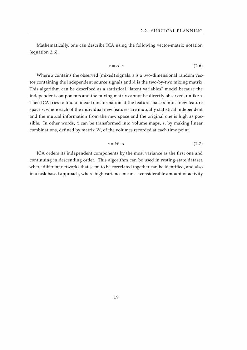
Mathematically, one can describe ICA using the following vector-matrix notation
(equation 2.6).
x = A · s (2.6)
Where x contains the observed (mixed) signals, s is a two-dimensional random vec-
tor containing the independent source signals and A is the two-by-two mixing matrix.
This algorithm can be described as a statistical “latent variables” model because the
independent components and the mixing matrix cannot be directly observed, unlike x.
Then ICA tries to find a linear transformation at the feature space x into a new feature
space s, where each of the individual new features are mutually statistical independent
and the mutual information from the new space and the original one is high as pos-
sible. In other words, x can be transformed into volume maps, s, by making linear
combinations, defined by matrix W , of the volumes recorded at each time point.
s =W · x (2.7)
ICA orders its independent components by the most variance as the first one and
continuing in descending order. This algorithm can be used in resting-state dataset,
where different networks that seem to be correlated together can be identified, and also
in a task-based approach, where high variance means a considerable amount of activity.
19

Chapter
3Materials and methods
This chapter is intended to explain how the current study was conducted, undergoing
a brief exposition of the software and methodology implemented. The chapter begins
with a description of the subjects who participated in the study as well as the parameters
of image acquisition. Then, detailed information about the methods and software used
in the pre-processing of the acquired data is reported, followed by the explanation of
the strategies used to process the images and to extract the activation networks of task
and rest paradigms. Finally, it is explained how the neural maps were superimposed
and its correlation calculation.
3.1 Participants and Image acquisition
This research gathered data provided by Hospital Cruz Vermelha. A total of 8 partici-
pants were recruited to participate in this study. All of them were previously referred for
surgical resection of a brain lesion. The demographic characteristics of the participants
are reported in table 3.1.
All patients were scanned using a 3-T (Philips Achieva by Philips Medical System,
Netherlands). A gradient echo sequence was applied and the first three volumes were
discarded in order to achieve a homogeneous magnetization. The data acquisition
protocol consists of the following steps.
Structural images were obtained with a matrix of 256x256, 160 contiguous slices,
voxel size of 1.8x1.8x4, flip angle = 8, repetition time (TR)=11ms and echo time
21

CHAPTER 3. MATERIALS AND METHODS
Table 3.1: Demographic features of the study population
Subject ID Sex Age
Sub001 M 19
Sub002 M 26
Sub003 M 37
Sub004 M 33
Sub005 M 14
Sub006 M 31
Sub007 M 32
Sub008 F 35
(TE)=4.6ms.
Functional images were acquired with a matrix of 128x128 and a flip angle of 90.
For the rs-fMRI acquisition the patient is requested to stare at a black screen, without
closing his eyes or making any other ocular movement. The scanning lasts 5 minutes, cor-
responding to 150 volumes of the entire brain. The voxel size was 2x2x3mm3,TR=2000
ms and TE=23 ms.
For the task paradigm the subjects had to perform blocks of tasks prompted by a
stimulus. The stimuli were displayed visually and required the ability to read. Language
tasks include detection of semantic and syntactic errors as well as sentence processing.
Language tasks paradigms consist of:
• Semantical Decision: detection of equals (=) or number signs (#) in the displayed
sentences. The sentences were presented according to 3 different frequencies (low,
medium, high), composed by two blocks each. Paradigm begins and ends with a
rest block.
• Synctatic Decision: 3 tested tasks: gender concordance, temporal conjugation and
the correct use of pronouns, each composed of two interleaved blocks. Paradigm
begins and ends with a rest block.
• Verb Generation: 4 blocks of linguistic stimuli interspersed with 4 blocks of visual
but not linguistic stimui, such as circles and number signs.
For semantic and syntactic paradigms, the number of volumes was 160, whereas for
the verb generation paradigm the number was 112. In both paradigms the voxel size
22
3.2. PREPROCESSING
was 2x2x4 TR was 2000ms and the TE was 23 ms .
In respect of motor tasks, these consist of:
• Mouth: 4 task blocks (opening and closing), interspersed with 4 rest blocks. The
paradigm begins with the completion of the task.
• Hand: 4 task blocks of hand bilateral motion, interspersed with 4 rest blocks. The
paradigm begins with the completion of the task.
• Feet: 4 task blocks of feet bilateral motion, interspersed with 4 rest blocks. The
paradigm begins with the completion of the task.
Task acquisitions comprises 80 holocranial volumes, a voxel size of 2x2x4, TR=3000
ms and TE= 33 ms.
3.2 Preprocessing
Data pre-processing was accomplished using a MATLAB® (The MathWorks Inc., MA,
USA version R2013a) implemented toolbox called Data Processing Assistant for Resting-
State fMRI- advanced edition (DPARSFA) (Chao-Gan and Yu-Feng, 2010). DPARSFA is
an user-friendly tool whithin Data Processing and Analysis for Brain Imaging (DPABI)
and it is based on some functions in Statistical Parametric Mapping (SPM) (developed
by members and collaborator of The Wellcome Trust Centre for Neuroimaging Institute
of Neurology, University College London) and Resting-State fMRI Data Analysis Toolkit
(REST) (Xiao-Wei Song, 2011). DPARSFA accepts structural and functional data in Dig-
ital Imaging and Communications in Medicine (DICOM) format, which is an universal
output format of fMRI scans.
The main purpose of this part of the study was essentially to choose the combination
of pre-processing parameters that best suited the ultimate goal, which was to recognize
and extract task and rest networks. The software template is displayed in fig 3.1.
The pre-processing was performed individually for each subject and one paradigm
at a time. Task data and rest data were pre-processed following different pipelines.
Below is described pre-processing steps on both cases.
• DICOM to Neuroimaging Informatics Technology Initiative (NIfTI)
The first step was to convert DICOM files to NIfTI format. This format includes
the affine coordinate system, which transforms voxel index (i,j,k) to spatial lo-
cation (x,y,z) and therefore gives the accurate information about where left and
23

CHAPTER 3. MATERIALS AND METHODS
Figure 3.1: DPARSFA layout
24

3.2. PREPROCESSING
right hemisphere is. In DPARSFA functional and structural data are converted
independently.
• Remove first time points In the scope of this study, it wasn’t required to discard
the first volumes since this has already been done as part of the standard acquisi-
tion procedure.
• Slice timing This option was checked with the purpose of correcting differences
in image acquisition time between slices.
Slice Number The slice number consists of 38 axial slices acquired contin-
uously for motion paradigms. In semantic, syntactic, verb generation and rest
paradigms the number of slices is 34.
Slice order Slices were acquired one by one from anterior to posterior, from
left to right and from bottom to top. Therefore, this option was filled with an
array going from 1 to number of slices.
Reference slice The reference slice was set to the slice acquired at halfway the
scan in order to reduce timing corrections.
• Realign - The realignment is applied by rigid body transformations, which as-
sumes that the shape and size of the volumes are the same and that one image can
be spatially matched to the first image, which SPM set it as reference, by the com-
bination of three translation (x,y,z; in mm) and three rotation parameters (pitch,
roll, yaw; in degrees). These operations are performed by matrices and can then
be multiplied together. See equation 3.1. Furthermore, one .txt file is created with
each volume’s motion specified for each axes and can be further applied as part of
nuisance regressor.
1 0 0 Xt
0 1 0 Yt
0 0 1 Zt
0 0 0 1
×
1 0 0 0
0 cosΦ sinΦ 0
0 −sinΦ cosΦ 0
0 0 0 1
×
cosΘ 0 sinΘ 0
0 1 0 0
−sinΘ 0 cosΘ 0
0 0 0 1
×
cosΩ sinΩ 0 0
−sinΩ cosΩ 0 0
0 0 1 0
0 0 0 1
(3.1)
• Voxel-Specific Head Motion The voxel-specific head motion is a nonlinear combi-
nation of the positions of the voxels and volume-wise translations and rotations.
25
CHAPTER 3. MATERIALS AND METHODS
Its goal is to minimize the difference of head motion impact on the voxels, depend-
ing on their distance from the center of the gradient coil. One text file is created
and comprises frame-wise displacements (FD) from the reference image for each
volume. This file is further applied in the scrubbing regressor calculation.
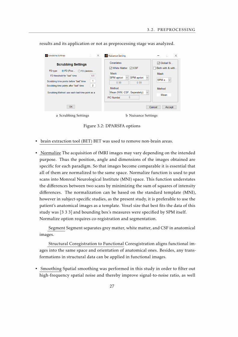
• Nuisance Covariates Regression Nuisance signals are those originating from non-
neural sources and can cause spurious activations.
Nuisance regressors Respiration and the cardiac signal are among the sources
of those artifactual signals. As these physiological sources are not recorded along
with the fMRI scan, it is possible to remove them based upon their frequency. For
this purpose nuisance covariates may include global mean signal (respiratory and
cardiac cycle), cerebrospinal fluid (CSF) and white matter (WM) signal, figure 3.2.
In this study all the covariates mentioned above were regressed out by GLM.
Head Motion Model In addition to physiological signal regressors, motion
regressors were added to GLM model. Those motion regressors included the 6
head motion parameters estimated in the realigment option, plus 6 head motion
parameters one time point before, and the 12 corresponding squared items, that
are all comprised in Friston 24-parameter model, (Friston et al., 1996 [34]).
Head motion scrubbing regressors As a final step, head motion scrubbing
regressors were generated to be further included in the model. The scrubbing
method identifies motion-induced spikes and rejects them based upon a defined
FD threshold. Of note that FD were previously estimated on voxel-specific head
motion option. In this study, the FD threshold for "bad" time point was 0.5 mm, i.e.
all the time points that were displaced 0.5 mm from the first time point considered
corrupted. According to the guidelines of Power et al. (2012b), the bad time points
as well as 1 before and 2 after neighbours were also excluded from data, figure 3.2.
DPARSFA produces one regressor for each time point excluded.
In conclusion, nuisance covariates removes physiological, non-neuronal noises
from data, and produces a matrix of regressors (or covariates) where each line
characterizes one time-point, and each column represents 24 motion parameters,
plus WM, CSF and global mean signal, and an undefined number of scrubbing
regressors.
Nuisance Covariates Regression is mentioned in the literature as being an ideal
method for pre-processing rest data [55]. Its contribution was tested in the final
26
3.2. PREPROCESSING
results and its application or not as preprocessing stage was analyzed.
a Scrubbing Settings b Nuisance Settings
Figure 3.2: DPARSFA options
• brain extraction tool (BET) BET was used to remove non-brain areas.
• Normalize The acquisition of fMRI images may vary depending on the intended
purpose. Thus the position, angle and dimensions of the images obtained are
specific for each paradigm. So that images become comparable it is essential that
all of them are normalized to the same space. Normalize function is used to put
scans into Monreal Neurological Institute (MNI) space. This function understates
the differences between two scans by minimizing the sum of squares of intensity
differences. The normalization can be based on the standard template (MNI),
however in subject-specific studies, as the present study, it is preferable to use the
patient’s anatomical images as a template. Voxel size that best fits the data of this
study was [3 3 3] and bounding box’s measures were specified by SPM itself.
Normalize option requires co-registration and segmentation.
Segment Segment separates grey matter, white matter, and CSF in anatomical
images.
Structural Coregistration to Functional Coresgistration aligns functional im-
ages into the same space and orientation of anatomical ones. Besides, any trans-
formations in structural data can be applied in functional images.
• Smoothing Spatial smoothing was performed in this study in order to filter out
high-frequency spatial noise and thereby improve signal-to-noise ratio, as well
27

CHAPTER 3. MATERIALS AND METHODS
as make the data more complying with the specifications of the underlying sta-
tistical theory (Gaussian Random Fields). This was accomplished by convolving
the images with a Gaussian kernel. In order to achieve the best pre-processing
pipeline, several kernel sizes were tested. From the matched filter theorem, the
best kernel size is about the same size as data activation. As it wasn’t known, at
the pre-processing stage, the precise size of activations, although it was known
that they wouldn’t be much significant, the size of the Gaussian that best suited
the study’s interest was a small one with full width at half maximum (FWHM) of 6
mm, which is in concordance with previous studies and follows a well-established
rule of thumb that suggests that the kernel width should be about 2 to 3 times
voxel size.
• Filter Temporal filtering was performed by a 0.01- 0.1 Hz bandpass filter, remov-
ing low-frequency drifts and physiological high-frequency respiratory and cardiac
signals.
• Detrend Several studies demonstrated the importance of removing linear trends
in voxel time courses in individual subjects. The origin of these trends is not com-
pletely understood, but they occur due to long-term physiological shifts. DPARSFA
relies on REST to estimate the linear trends with a least-square fitting of a straight
line, which is removed from the data. Subsequently, the original mean value of
each time course is added back.
• Scrubbing To save computational time, scrubbing option was not performed in
pre-processing stage, since it was previously included as a regressor on nuisance
matrix.
3.3 Processing
Task data was processed whith SPM, while rest data was processed with Group ICA of
fMRI toolbox (GIFT).
3.3.1 Task data - Statistical Analysis
In order to reliably detect voxels activated by task paradigms, statistical data analysis
was performed by GLM in SPM, consult subsection 2.2.4.3.
28
3.3. PROCESSING
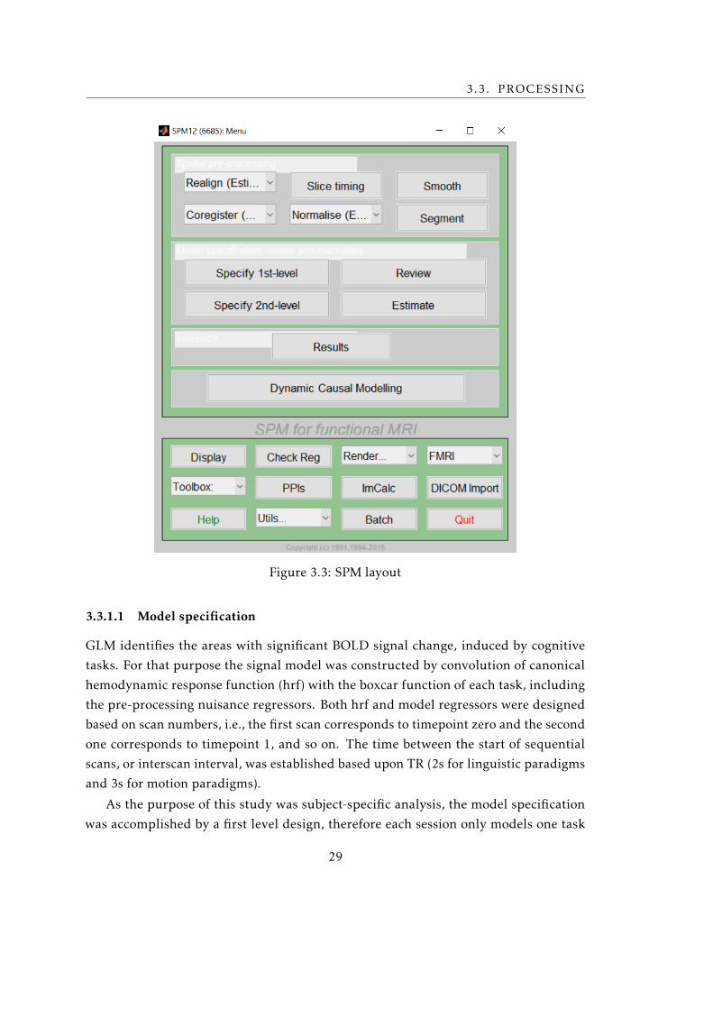
Figure 3.3: SPM layout
3.3.1.1 Model specification
GLM identifies the areas with significant BOLD signal change, induced by cognitive
tasks. For that purpose the signal model was constructed by convolution of canonical
hemodynamic response function (hrf) with the boxcar function of each task, including
the pre-processing nuisance regressors. Both hrf and model regressors were designed
based on scan numbers, i.e., the first scan corresponds to timepoint zero and the second
one corresponds to timepoint 1, and so on. The time between the start of sequential
scans, or interscan interval, was established based upon TR (2s for linguistic paradigms
and 3s for motion paradigms).
As the purpose of this study was subject-specific analysis, the model specification
was accomplished by a first level design, therefore each session only models one task
29

CHAPTER 3. MATERIALS AND METHODS
Figure 3.4: fMRI model specification
paradigm for one subject. In the context of feet, hands, mouth and verb generation
paradigms, only one boxcar condition was defined per session, since those cases re-
flected on-off stimulation paradigms. On the other hand, 4 conditions were setted for
each semantic and syntactic task. As regards to semantic decision, the 4 conditions
describe the 3 frequencies of the stimuli (low, medium, high) and the free-stimulus
condition at the beginning and end of the task. Relatively to syntactic decision, the 4
conditions were gender concordance, temporal conjugation an correct use of pronouns,
including the free-stimulus condition at the beginning and end of the task. The onset
times and the period of the stimulation were specified in the SPM framework.
As regards to other predictors to be implemented, two distinct processes were fol-
lowed depending on whether pre-processing included nuisance covariates regression
30

3.3. PROCESSING
or not. In the first case, a multiple regression was performed resorting to nuisance
covariates matrix created in the pre-processing stage. On the other hand, head motion
regressors were included in the model through realignment parameters’ text file and
an additional regressor in cases where the subject performed to much movement. The
latter array was created using MATLAB® functions and attempted to reproduce head
motion scrubbing regressor. For this purpose, the construction of the array resorted on
the framewise displacement of each volume. If the displacement was higher than 0.5
mm then that volume, such as the one before and the two after adjacent volumes were
excluded, ie were represent by an ‘0’ in the vector. The remaining volumes acquire the
value ‘1’.
Masking data aims to only estimate voxels that seem to have significant signal in
them. As for the default SPM sets masking threshold threshold to 0.8, which means that
the model is estimated based on voxels whose mean value is at 80% of the global signal.
However if nuisance covariates regression formed an integral part of the pre-processing,
this threshold has to be setted to -inf. As the significance of the activation voxels is low,
mask that include all brain, and not a specific portion, was applied.
3.3.1.2 β estimation and contrast
After the model be established, GLM estimated β values using an autoregressive model
during restricted maximum likelihood (ReML) parameter estimation, which assumes
that each voxel has the same error correlation structure.
Once β were estimated, we tested if the most significant β were assigned to the most
important regressors of the model, in other words, if the most important regressor was
greater than 0. Within the context of this experiment, the most important regressors
were the ones that describe the defined conditions. To test that, we relied on GLM
T-contrasts to define the hypothesis and t-test to assess it.
In GLM, a contrast specifies linear combinations of β. In motion paradigms context,
as only one on-off condition was defined for each motion, a simple contrast was applied.
[1 0 0 · · · 0n
]Where n is the number of regressors.
In the case of semantic and syntactic paradigms, a weighted contrast between the
different conditions, plus a -1 weighted, to ensure that the sum of weights was zero, was
established, like the following array.
31
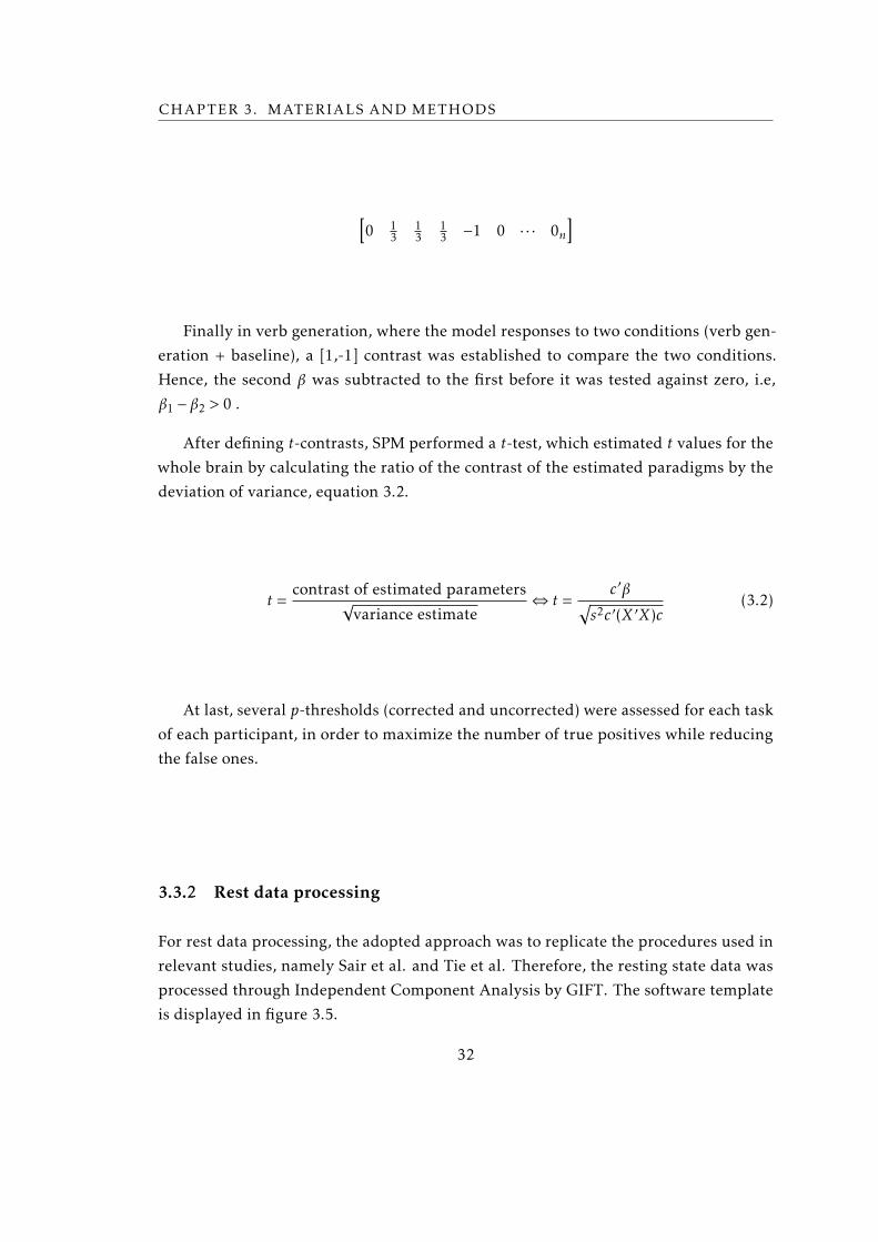
CHAPTER 3. MATERIALS AND METHODS
[0 1
313
13 −1 0 · · · 0n
]
Finally in verb generation, where the model responses to two conditions (verb gen-
eration + baseline), a [1,-1] contrast was established to compare the two conditions.
Hence, the second β was subtracted to the first before it was tested against zero, i.e,
β1 − β2 > 0 .
After defining t-contrasts, SPM performed a t-test, which estimated t values for the
whole brain by calculating the ratio of the contrast of the estimated paradigms by the
deviation of variance, equation 3.2.
t =contrast of estimated parameters
√variance estimate
⇔ t =c′β√
s2c′(X ′X)c(3.2)
At last, several p-thresholds (corrected and uncorrected) were assessed for each task
of each participant, in order to maximize the number of true positives while reducing
the false ones.
3.3.2 Rest data processing
For rest data processing, the adopted approach was to replicate the procedures used in
relevant studies, namely Sair et al. and Tie et al. Therefore, the resting state data was
processed through Independent Component Analysis by GIFT. The software template
is displayed in figure 3.5.
32

3.4. COMPARISON OF TASK NETWORKS AND RESTING STATE NETWORKS
Figure 3.5: GIFT layout
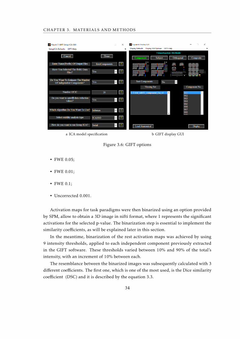
Just like the studies mentioned above, components were estimated for each subject
using the minimum description length (MDL) criteria. ICA maps were generated for
20 and 50 independent components using Infomax algorithm. In order to determine
the reliance and stability of the previously selected ICA algorithm, ICASSO toolbox was
applied. ICA algorithm ran 5 times, and each run started with a different initial value
(RandInit), figure 3.6.
The extracted independent components were then visually assessed using the soft-
ware display option, figure 3.6
.
3.4 Comparison of Task Networks and Resting State Networks
In order to evaluate how rest activation maps are related to task activation maps, differ-
ent similarity coefficients were employed. The precedent procedures that characterize
this analysis are described below.
For each task of each participant, 4 different activation maps were created in SPM.
Each map resulted from the application of the following different significance levels:
33
CHAPTER 3. MATERIALS AND METHODS
a ICA model specification b GIFT display GUI
Figure 3.6: GIFT options
• FWE 0.05;
• FWE 0.01;
• FWE 0.1;
• Uncorrected 0.001.
Activation maps for task paradigms were then binarized using an option provided
by SPM, allow to obtain a 3D image in nifti format, where 1 represents the significant
activations for the selected p-value. The binarization step is essential to implement the
similarity coefficients, as will be explained later in this section.
In the meantime, binarization of the rest activation maps was achieved by using
9 intensity thresholds, applied to each independent component previously extracted
in the GIFT software. These thresholds varied between 10% and 90% of the total’s
intensity, with an increment of 10% between each.
The resemblance between the binarized images was subsequently calculated with 3
different coefficients. The first one, which is one of the most used, is the Dice similarity
coefficient (DSC) and it is described by the equation 3.3.
34

3.4. COMPARISON OF TASK NETWORKS AND RESTING STATE NETWORKS
DSC = 2|R∩ T ||R|+ |T |
(3.3)
The numerator is the overlap between the activations of rest (R) and task (T ) bina-
rized maps, and the denominator is the sum of both.
This coefficient takes values between 0 and 1, wherein 1 is the perfect overlap,
whereas 0 describes the opposite event. A low value of the DSC can represent one of
two situations: the intersection of rest and task activations is low or the union between
the two activations is high. As the reason why Dice coefficient might be low can not be
directly measured by this index it became necessary to create two more indexes.
One of them, equation 3.4, is a measure of the overlap of rest activation maps on task
activation maps, ie, if the index has the value 1, means that all task activations match rest
activations, however does not directly imply that all the rest activations coincide with
task activations. This coefficient, will be henceforth designated by Similarity Coefficient
1 (or SC1).
SC1 =|R∩ T ||T |
(3.4)
Lastly, equation 3.5 attempts to find the contribution of rest activations in the over-
lap of the two maps. This coefficient, will be hereinafter designated by Similarity Coef-
ficient 2 (or SC2). If this index is close to 1 it means that there are no coincidences on
where the rest and task activations take place.
SC2 =
∣∣∣R∩ T ∣∣∣|R|
(3.5)
The next scheme aims to lay out some of the most important steps in pre-processing,
processing, and data analysis.
35
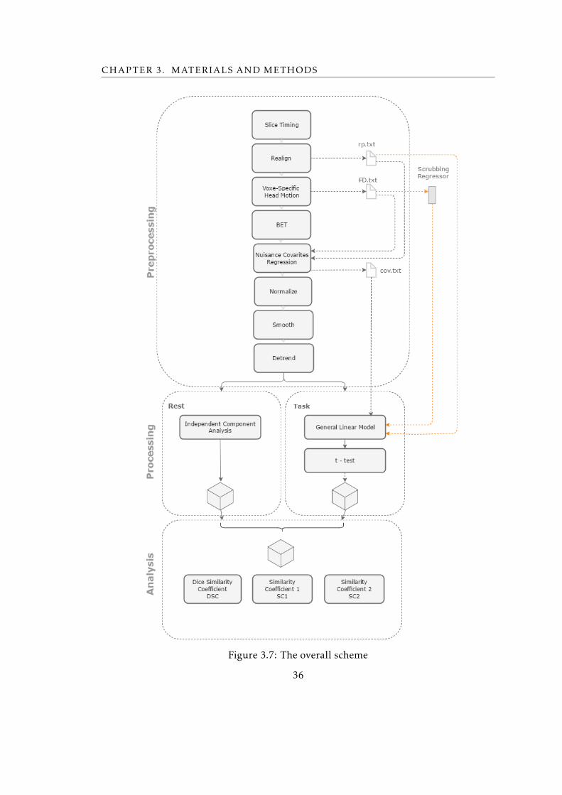
CHAPTER 3. MATERIALS AND METHODS
Figure 3.7: The overall scheme
36
Chapter
4Results
This chapter is intended to report the most relevant results obtained in pre-processing
and processing stages, followed by the presentation of statistical and similarity analysis
results. Due to the large volume of data, results from the latter will be presented in
two different approaches. One intends to present the outcomes of all tasks for a single
participant, and the other approach aims to present the results of one single task for all
subjects. The selection criterion of the subject and task to present in this section is the
minimum number of volume removed by the scrubbing procedure.
4.1 Important results from preprocessing
As the design of a preprocessing protocol was a key part of this research, herein are the
results of some of the parameters which arouse more questions.
4.1.1 Scrubbing
The amount of volumes removed by scrubbing method is presented in the table 4.1. It is
important to emphasize that the volumes presented in the chart comprise the ones that
have a framewise displacement greater than the value stipulated by Power et al. [56] as
well as the preceding volume and the following two. They were regressed out from a
total of 80 volumes in motor paradigms, 160 in semantic and syntactic decision, 112 in
verb generation and finally 150 in rest.
37

CHAPTER 4. RESULTS
From the information presented in the table, it is possible to affirm that subject
003 is the one with fewer volumes removed, alongside with Sub006. For the first one,
only hands motor paradigm led to a framewise displacement greater than the value
stipulated by Power et al., while in the second one volumes were withdrawn only in the
syntactic decision. Subject 005 is the one with the largest number of volumes removed,
since in all tasks, and rest included, several volumes had to be regressed out. Another
finding worth mentioning is the major impact of scrubbing on language paradigms for
subject 001 and 002, since only 10 time points remain in each paradigm.
Regarding to tasks, the feet paradigms are noted for producing the largest number
of removals between the motor tasks, while the semantic decision stands out among the
linguistics. In rest, few or none volumes were removed, excepting for Sub005.
Table 4.1: Scrubbing Results
SubjectID
Motor Paradigms Linguistic ParadigmsRest
Mouth Hands FeetSemanticDecision
SyntacticDecision
VerbGeneration
Sub001 0 10 0 150 150 150 0Sub002 4 0 34 150 150 150 4Sub003 0 4 0 0 0 0 0Sub004 14 0 0 0 0 0 0Sub005 55 51 62 150 85 30 56Sub006 0 0 0 0 13 0 4Sub007 0 0 12 0 4 0 4Sub008 0 4 0 36 9 27 4
4.1.2 Normalization
As mentioned in section 3.2, the image acquisition is different for motor tasks and for
rest and language tasks. This difference is more evident in the images dimensions.
The dimensions of motor tasks images are 128x128x38 while rest and language tasks
images have a dimension of 128x128x34, which results in an inconsistent comparison
and in the impracticability of similarity analysis between the motor tasks data and rest.
To illustrate this difference, the figure 4.1 contains a representation of mouth task
image and semantic decision of Sub003 immediately before and after normalization to
Montreal Neurological Institute (MNI) space.
38
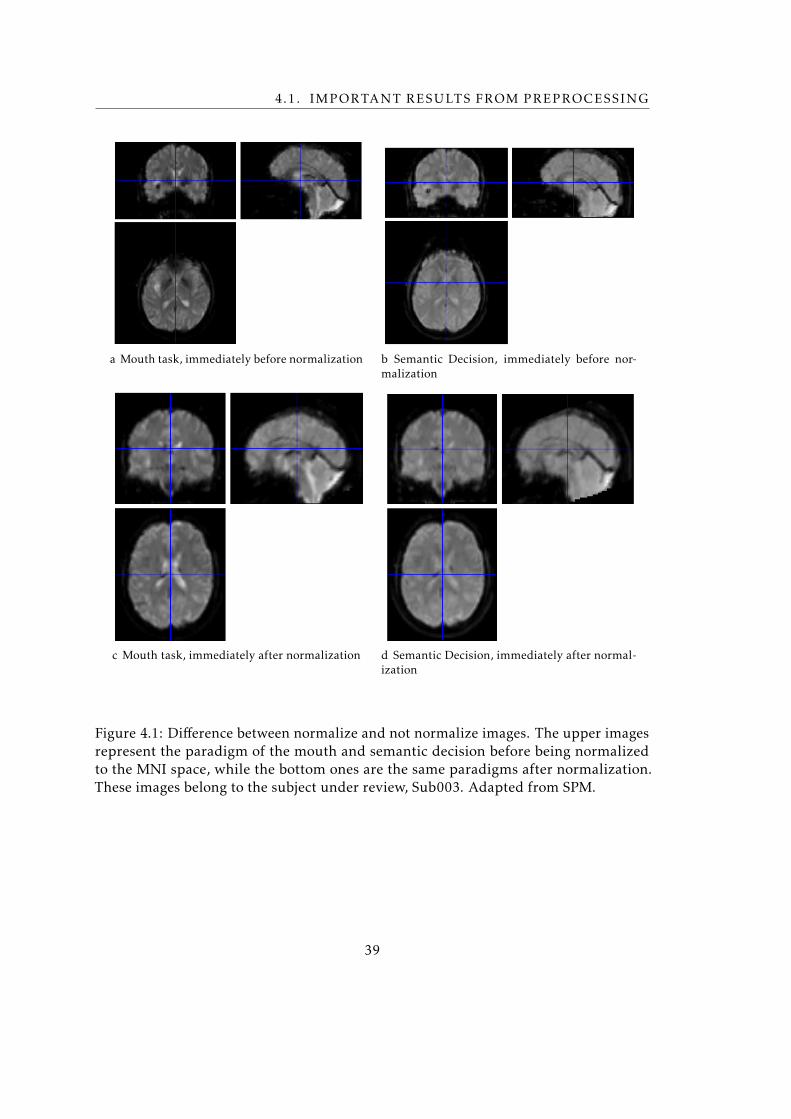
4.1. IMPORTANT RESULTS FROM PREPROCESSING
a Mouth task, immediately before normalization b Semantic Decision, immediately before nor-malization
c Mouth task, immediately after normalization d Semantic Decision, immediately after normal-ization
Figure 4.1: Difference between normalize and not normalize images. The upper imagesrepresent the paradigm of the mouth and semantic decision before being normalizedto the MNI space, while the bottom ones are the same paradigms after normalization.These images belong to the subject under review, Sub003. Adapted from SPM.
39

CHAPTER 4. RESULTS
4.1.3 Removal of nuisance signals
The removal of the nuisance signals includes removing all non-neuronal signals and pro-
duces the visual effect illustrated in fig 4.2. The sub figure related to the performance
of this procedure is much more blurred than one that not contemplates it.
Despite the removal of nuisance signals produce an overly blur effect it is not auto-
matically indicative of a worse activations extraction. Thus, to test the efficiency of this
procedure two analysis were carried out in parallel, one using this procedure and the
other not. The results of these two analysis are available in section 4.2.1.1.
a Mouth task, immediately before removing nui-sance signal
b Mouth task, immediately after removing nui-sance signal
Figure 4.2: Effect of nuisance signals removal. These images belong to the subject underreview, Sub003. Adapted from SPM.
40

4.2. INTRA-SUBJECT ANALYSIS
4.2 Intra-Subject Analysis
This section aims to present the results in an intra-subject perspective. Thus, the results
of activations mapping of all task paradigms and at rest will be presented for subject
003. The choice of this subject, as mentioned earlier in this chapter, is related to the
small number of volumes removed by scrubbing (consult table 4.1).
4.2.1 Motor Paradigms
4.2.1.1 Mouth paradigms
As described in section 3.4, similarity tests were conducted by resorting to 4 distinct
maps coming from Statistical Parametric Mapping SPM. Each map results from a differ-
ent significance level. The visual effect of selecting different p-values can be found in
figure 4.3.
41

CHAPTER 4. RESULTS
a FWE p < 0.01 b FWE p < 0.05
c FWE p < 0.1 d UNC p < 0.001
Figure 4.3: SPM activations map resulting from mouth paradigm of Sub003. Each maprepresents the activation using a distinct p-value. Mouth activation with a) p-valueinferior to 0.01 FWE; b) p-value inferior to 0.05 FWE c) p-value inferior to 0.1 FWE; d)p-value inferior to 0.001 uncorrected;
The first three images are listed in ascending order of p-values with familywise error
FWE correction (FWE), whereas the image at the bottom right has an uncorrected p-
value of 0.001. For more conservative levels of significance the number of activations is
smaller than in the case where no corrections were performed along with the statistical
tests.
SPM displays images in neurological convention, which means that the left side of
42

4.2. INTRA-SUBJECT ANALYSIS
the image corresponds to the left side of the brain. In this specific case, functional im-
ages were superposed with structural images specific to the subject, in order to improve
the perception of regions where activations take place.
From the figures it is clear that there is bilateral activation in the ventral portion of
the precentral gyrus, immediately above the Sylvian fissure. Additionally, in the bottom
right image it is possible to distinguish an activation below the Sylvian fissure. SPM
enables the visualization of the activations, as well as presents the designed model and
a table with the relevant statistical values, figure 4.4. Among other information, the
table presents the statistical significance of voxel intensity (“peak level”), which was
the approach used in this study, but also presents the statistical values related to cluster
extent (“cluster level”) and a global p-value related to the whole map which combines
intensity and extent information and reflects the likelihood of getting the activation
pattern by chance (“set level”). Uncorrected p-values are shown alongside p-values
corrected using FWE and False Discovery Rate (a less strict method).
From the 50 independent components extracted by the Group ICA of fMRI toolbox,
GIFT software, the 5 wich most resemble task activations were selected. Thereunto, one
correlation map between the binarized activation maps of all independent components
and task activation maps was used to infer the most relevant components for the study.
This procedure was repeated for each p-value activation map for each similarity test,
accounting for a total of 12 colormaps for each task.
Taking the example highlighted in this section, and considering only the correlation
map in the case of a p-value < 0.05 (FWE) and the Dice similarity coefficient (DSC)
test, the most significant independent components for mouth motion paradigm were IC
number 33, 21, 50, 19 and 3, as shown in figure 4.5.
In order to ensure a proper analysis of the data, the maps of the most important
independent component (IC) were visually evaluated, figure 4.6. The image was directly
extracted from the GIFT environment, whereat it not reflects the intensity threshold
that was applied to it.
The figure consists of several transverse planes of the brain ordered from superior
planes to inferior ones. In the superior planes, activations are located over the coronal
plane. As the planes become more inferior, activations emerge in the sagittal plane and
for planes even further inferior activations become bilateral. Along planes it is possible
to evidence the existence of residual activations scattered throughout the brain.
43

CHAPTER 4. RESULTS
Figure 4.4: SPM environment. In the upper left corner, there is the map of activations.In the upper right corner is displayed the designed model matrix.And in the bottom ofthe image is presented the statistical table
44

4.2. INTRA-SUBJECT ANALYSIS
Figure 4.5: Correlation map of IC extracted from rest data with different intensitythresholds, for mouth activation map of Sub003, with a p-value < 0.05 FWE. The y-axisrepresents each of independent components and the x-axis is the intensity threshold,with 1 corresponding to 10% and 9 corresponding to 90% of maximum intensity. Themost significant IC are 3, 21, 50, 19 and 3.
The results of the similarity tests between resting-state and task activation maps
are displayed in table 4.2. Due to the high amount of data, the results presented in
the table expound the 5 best outcomes. Dice Similarity Coefficient(DSC) has the lowest
correlation values among the 3 similarity coefficients, whereas the Similarity Coefficient
2 has the highest outcomes. In a general overview, the similarity values of DSC increase
for p-values less conservative, while SC1 and SC2values decrease. The increase in DSC
values means that the performance of too restrictive statistical thresholds leads to the
removal of activated task regions that are coincident with the activated regions in resting
state. The decline in the latter coefficients derives from the increased activated mouth
regions as result of application of a low restrictive statistical threshold.
45

CHAPTER 4. RESULTS
Figure 4.6: Independent Component of Sub003 rest network obtained in GIFT software.The figure consists of several transverse planes of the brain ordered from superior planesto inferiors.
46

4.2. INTRA-SUBJECT ANALYSIS
Table 4.2: Similarity results for rest activation maps and mouth paradigm activationmaps for Sub003.
ICIntensity
ThresholdDSC
(max)IC
IntensityThreshold
SC1(max)
ICIntensity
ThresholdSC2
(min)
FWE0.01
33 0.1 0.0032 33 0.1 0.8387 33 0.1 0.998450 0.1 0.0025 50 0.1 0.7742 50 0.1 0.998721 0.1 0.0023 3 0.1 0.6774 21 0.1 0.99893 0.2 0.0018 35 0.1 0.5484 3 0.2 0.99913 0.3 0.0017 3 0.2 0.5161 3 0.3 0.9992
FWE0.05
33 0.1 0.0058 33 0.1 0.7619 33 0.1 0.997121 0.1 0.0048 50 0.1 0.6508 21 0.1 0.997650 0.1 0.0043 3 0.1 0.6191 19 0.4 0.997819 0.4 0.0039 35 0.1 0.5714 50 0.1 0.99783 0.2 0.0032 3 0.2 0.4762 19 0.2 0.9983
FWE0.1
19 0.3 0.0076 33 0.1 0.7342 19 0.4 0.995633 0.1 0.0070 50 0.1 0.670.9 33 0.1 0.996519 0.4 0.0061 35 0.1 0.5696 19 0.3 0.996719 0.2 0.0060 3 0.1 0.5443 19 0.2 0.996950 0.1 0.0056 3 0.2 0.4177 50 0.1 0.9972
UNC0.001
19 0.3 0.0357 35 0.1 0.5318 33 0.7 0.970619 0.4 0.0301 33 0.1 0.5202 19 0.4 0.973419 0.2 0.0249 50 0.1 0.4884 33 0.5 0.973635 0.4 0.0226 3 0.1 0.4711 33 0.6 0.976221 0.1 0.0221 21 0.1 0.3150 19 0.3 0.9771
• Similarity test without nuisance signals
All procedures described above were repeated for the data from the nuisance
signal removal. The overall result of the similarity tests are shown in table 4.3.
For the most restrictive threshold of p-value, no value of DSC was greater than
0. This outcome stems from a null intersection of task and rest activations maps,
which may mean not only that activations do not overlap as at least one of the
maps does not include any activation. As regards to the SC1, all the results were
an indeterminate form 00 , which means that the applied statistical threshold was
too severe, and no activation remained in the task map. Finally, no SC2 was
different from 1 thus ensuring the existence of activations at rest.
As for the others p-values, the results express the same pattern verified in data
with nuisance signals, namely the very low values of DSC and very high values of
SC2. The maximum value observed in some cases of SC1, results from the absolute
overlap of the rare regions activated in the task with rest areas.
47

CHAPTER 4. RESULTS
As the results obtained with the extraction of nuisance signals proved to be worse
than the ones which arises from images within nuisance signals, study was con-
ducted using only the latter.
Table 4.3: Similarity results for rest activation maps and mouth paradigm activationmaps for Sub003, with nuisance signals removal.
ICIntensity
ThresholdDSC
(max)IC
IntensityThreshold
SC1(max)
ICIntensity
ThresholdSC2
(min)
FWE0.01
0 - 1
FWE0.05
42 0.1 0.0003 18 0.1 1.0000 42 0.1 0.999818 0.1 0.0002 28 0.1 1.0000 18 0.1 0.999943 0.1 0.0002 42 0.1 1.0000 43 0.1 0.999928 0.1 0.0001 43 0.1 1.0000 28 0.1 0.9999- - - - - - - - -
FWE0.1
18 0.3 0.0015 18 0.1 1.0000 18 0.3 0.999218 0.2 0.0012 6 0.1 0.8000 18 0.2 0.999418 0.1 0.0009 45 0.1 0.6000 18 0.1 0.999536 0.1 0.0006 18 0.2 0.4000 36 0.1 0.99976 0.1 0.0006 28 0.1 0.4000 6 0.1 0.9997
UNC0.001
18 0.2 0.0116 18 0.1 0.3072 18 0.2 0.993918 0.1 0.0093 19 0.1 0.1867 18 0.1 0.995318 0.3 0.0080 6 0.1 0.1687 18 0.3 0.995536 0.1 0.0078 25 0.1 0.1687 22 0.3 0.995940 0.1 0.0071 45 0.1 0.1687 40 0.3 0.9959
The procedure performed to test similarity between resting-state networks and
mouth paradigm networks was reproduced for the remaining 5 tasks.
48

4.2. INTRA-SUBJECT ANALYSIS
4.2.1.2 Hand
The results of applying different statistical thresholds to the paradigm hand data is
represented in the figure 4.7.
As in mouth activation maps, for more restrictive p-values and its correction, the
number of activations is smaller than in the case where no corrections were performed
along with the statistical tests. The activation is bilateral, with a clear dominance of the
right hemisphere since its expression is evident for less restrictive statistical corrections.
The activation area emerged in the upper regions of precentral and postcentral gyrus.
a FWE p < 0.01 b FWE p < 0.05
c FWE p < 0.1 d uncorrected p < 0.01
Figure 4.7: The 4 images at the top represent mouth activation with distinct p-values a)p-value inferior to 0.01 FWE; b) p-value inferior to 0.05 FWE; c) p-value inferior to 0.1FWE; d) p-value inferior to 0.001 uncorrected.
The independent component that best overlaps the hand activation map is repre-
sented in figure 4.8. It is possible to recognize a strong activation in higher regions of
the cortex, which disperse as the plane includes lower portions of the brain.
49

CHAPTER 4. RESULTS
Figure 4.8: Independent Component of Sub003 rest network obtained in GIFT software.The figure consists of several transverse planes of the brain ordered from superior planesto inferiors.
The results of the similarity tests between resting-state and hands activation maps
are displayed in table 4.2. The observed pattern repeats the tendency explained in the
previous section, 4.2.1.1 .
50
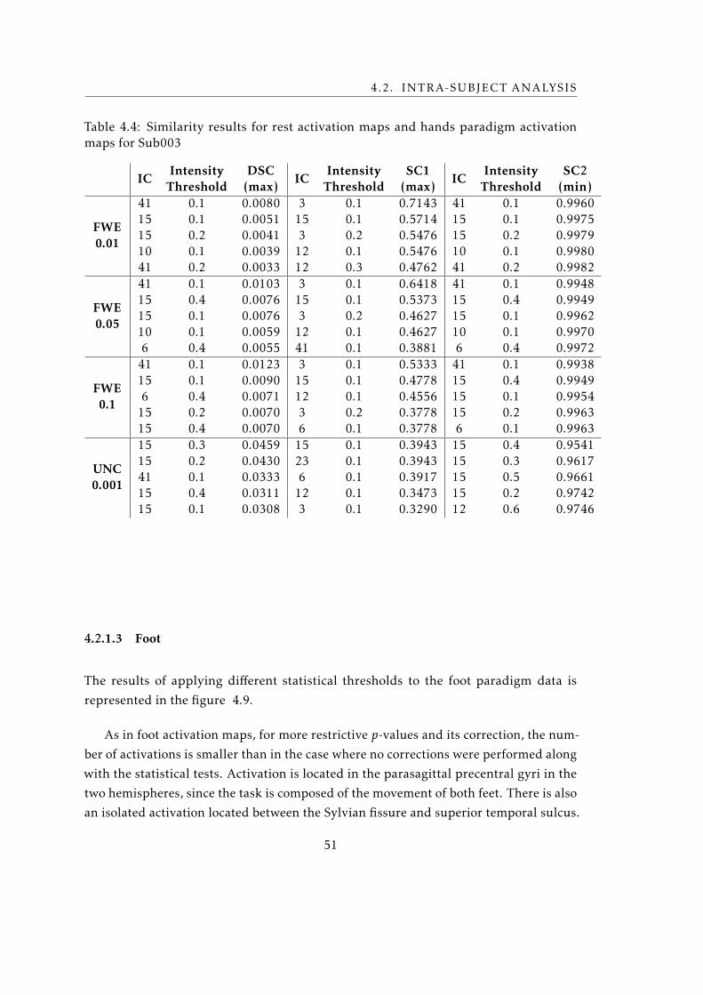
4.2. INTRA-SUBJECT ANALYSIS
Table 4.4: Similarity results for rest activation maps and hands paradigm activationmaps for Sub003
ICIntensity
ThresholdDSC
(max)IC
IntensityThreshold
SC1(max)
ICIntensity
ThresholdSC2
(min)
FWE0.01
41 0.1 0.0080 3 0.1 0.7143 41 0.1 0.996015 0.1 0.0051 15 0.1 0.5714 15 0.1 0.997515 0.2 0.0041 3 0.2 0.5476 15 0.2 0.997910 0.1 0.0039 12 0.1 0.5476 10 0.1 0.998041 0.2 0.0033 12 0.3 0.4762 41 0.2 0.9982
FWE0.05
41 0.1 0.0103 3 0.1 0.6418 41 0.1 0.994815 0.4 0.0076 15 0.1 0.5373 15 0.4 0.994915 0.1 0.0076 3 0.2 0.4627 15 0.1 0.996210 0.1 0.0059 12 0.1 0.4627 10 0.1 0.99706 0.4 0.0055 41 0.1 0.3881 6 0.4 0.9972
FWE0.1
41 0.1 0.0123 3 0.1 0.5333 41 0.1 0.993815 0.1 0.0090 15 0.1 0.4778 15 0.4 0.99496 0.4 0.0071 12 0.1 0.4556 15 0.1 0.9954
15 0.2 0.0070 3 0.2 0.3778 15 0.2 0.996315 0.4 0.0070 6 0.1 0.3778 6 0.1 0.9963
UNC0.001
15 0.3 0.0459 15 0.1 0.3943 15 0.4 0.954115 0.2 0.0430 23 0.1 0.3943 15 0.3 0.961741 0.1 0.0333 6 0.1 0.3917 15 0.5 0.966115 0.4 0.0311 12 0.1 0.3473 15 0.2 0.974215 0.1 0.0308 3 0.1 0.3290 12 0.6 0.9746
4.2.1.3 Foot
The results of applying different statistical thresholds to the foot paradigm data is
represented in the figure 4.9.
As in foot activation maps, for more restrictive p-values and its correction, the num-
ber of activations is smaller than in the case where no corrections were performed along
with the statistical tests. Activation is located in the parasagittal precentral gyri in the
two hemispheres, since the task is composed of the movement of both feet. There is also
an isolated activation located between the Sylvian fissure and superior temporal sulcus.
51
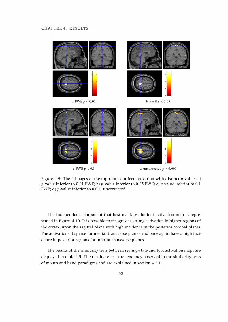
CHAPTER 4. RESULTS
a FWE p < 0.01 b FWE p < 0.05
c FWE p < 0.1 d uncorrected p < 0.001
Figure 4.9: The 4 images at the top represent feet activation with distinct p-values a)p-value inferior to 0.01 FWE; b) p-value inferior to 0.05 FWE; c) p-value inferior to 0.1FWE; d) p-value inferior to 0.001 uncorrected.
The independent component that best overlaps the foot activation map is repre-
sented in figure 4.10. It is possible to recognize a strong activation in higher regions of
the cortex, upon the sagittal plane with high incidence in the posterior coronal planes.
The activations disperse for medial transverse planes and once again have a high inci-
dence in posterior regions for inferior transverse planes.
The results of the similarity tests between resting-state and foot activation maps are
displayed in table 4.5. The results repeat the tendency observed in the similarity tests
of mouth and hand paradigms and are explained in section 4.2.1.1
52

4.2. INTRA-SUBJECT ANALYSIS
Figure 4.10: Independent Component of Sub003 rest network obtained in GIFT software.The figure consists of several transverse planes of the brain ordered from superior planesto inferiors.
53

CHAPTER 4. RESULTS
Table 4.5: Similarity results for rest activation maps and feet paradigm activation mapsfor Sub003
ICIntensity
ThresholdDSC
(max)IC
IntensityThreshold
SC1(max)
ICIntensity
ThresholdSC2
(min)
FWE0.01
2 0.2 0.0208 2 0.1 1 2 0.2 0.98952 0.3 0.0118 6 0.1 0.9546 2 0.3 0.99402 0.1 0.0109 7 0.1 0.8182 2 0.1 0.99452 0.4 0.0089 2 0.2 0.7727 2 0.4 0.99537 0.3 0.0086 6 0.2 0.7273 7 0.3 0.9956
FWE0.05
2 0.2 0.0384 2 0.1 0.8600 2 0.2 0.98022 0.3 0.0319 6 0.1 0.8600 2 0.3 0.98312 0.4 0.0294 7 0.1 0.7200 2 0.4 0.98362 0.5 0.0222 6 0.2 0.6600 2 0.5 0.98642 0.1 0.0211 2 0.2 0.6400 2 0.1 0.9893
FWE0.1
2 0.2 0.05 2 0.1 0.8594 2 0.2 0.97402 0.3 0.0426 6 0.1 0.8594 2 0.4 0.97652 0.4 0.0408 7 0.1 0.7031 2 0.3 0.97702 0.1 0.0269 6 0.2 0.6719 2 0.1 0.98647 0.3 0.0232 2 0.2 0.6563 2 0.5 0.9864
UNC0.001
2 0.3 0.1079 6 0.1 0.5497 2 0.4 0.92492 0.2 0.1053 2 0.1 0.4596 2 0.3 0.92502 0.4 0.0856 49 0.1 0.4317 2 0.2 0.93692 0.1 0.0680 7 0.1 0.3975 2 0.5 0.94097 0.3 0.0505 6 0.2 0.3882 15 0.4 0.9592
4.2.1.4 Multi-motor task
Since there is no resting state network that resembles with only one motor tasks de-
scribed above, a map resulting of overlapping mouth, hand and foot activated regions
was created. The results of that test are displayed in table 4.6. The displayed pattern
repeats the individual tendency of each task, which is, Dice Similarity Coefficient (DSC)
has the lowest correlation values among the 3 similarity coefficients, whereas the Simi-
larity Coefficient 2 has the highest outcomes. The similarity values of DSC increase for
p-values less conservative, while SC1 and SC2values decrease.
The great difference that exists is the loss of sensitivity, i.e., the SC1 is lower in the
overlapping than in each task individually.
54

4.2. INTRA-SUBJECT ANALYSIS
Table 4.6: Similarity test results for rest activation maps and with the result of thesuperposition of the 3 motor tasks for Sub003
ICIntensity
ThresholdDSC
(max)IC
IntensityThreshold
SC1(max)
ICIntensity
ThresholdSC2
(min)
FWE0.01
2 0.2 0.0199 3 0.1 0.5368 2 0.2 0.98952 0.3 0.0108 33 0.1 0.4737 2 0.3 0.99402 0.1 0.0107 12 0.1 0.4211 2 0.1 0.9945
15 0.2 0.0100 3 0.2 0.4105 15 0.2 0.994741 0.1 0.0087 35 0.1 0.3895 2 0.4 0.9953
FWE0.05
2 0.2 0.0356 3 0.1 0.4778 2 0.2 0.98022 0.3 0.0278 33 0.1 0.4389 2 0.3 0.98312 0.4 0.0231 35 0.1 0.4000 2 0.4 0.98362 0.1 0.0204 6 0.1 0.3889 2 0.5 0.9864
15 0.2 0.0183 3 0.2 0.3611 2 0.1 0.9893
FWE0.1
2 0.2 0.0454 33 0.1 0.4249 2 0.2 0.97402 0.3 0.0358 3 0.1 0.4163 2 0.4 0.97652 0.4 0.0303 6 0.1 0.4034 2 0.3 0.97702 0.1 0.0263 35 0.1 0.3863 2 0.1 0.9861
15 0.2 0.0244 15 0.1 0.3476 15 0.2 0.9863
UNC0.001
2 0.2 0.0859 33 0.1 0.3983 15 0.4 0.91842 0.3 0.0719 6 0.1 0.3655 2 0.3 0.91902 0.1 0.0703 3 0.1 0.3539 2 0.4 0.9249
15 0.2 0.0675 35 0.1 0.3250 15 0.3 0.925215 0.3 0.0533 50 0.1 0.2970 2 0.2 0.9295
55

CHAPTER 4. RESULTS
4.2.2 Language
4.2.2.1 Semantic Decisions
The semantic decisions of this subject produced no significant activations, so the assess-
ment of the similarity between task activated maps and rest maps is meaningless.
4.2.2.2 Syntactic Decisions
The results of applying different statistical thresholds to the syntactic paradigm data is
represented in the figure 4.11.
For more restrictive p-values and its correction, the number of activated regions is
smaller than in the case where no corrections were performed along with the statistical
tests.
The activation produced by syntactical decision is robust. For lower axial planes,
is evident a bilateral activation located in the middle temporal gyrus, illustrated in
subfigures a, b, c (figure 4.11). For superior axial planes there is a great activation near
the Broca’s area in the right hemisphere and a small activation close to the Wernicke’s
area in the contralateral hemisphere. It is also important to mention that the cerebellum
is another area with prominent activation.
56
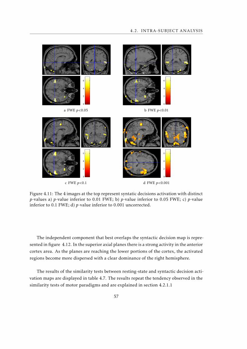
4.2. INTRA-SUBJECT ANALYSIS
a FWE p<0.05 b FWE p<0.01
c FWE p<0.1 d FWE p<0.001
Figure 4.11: The 4 images at the top represent syntatic decisions activation with distinctp-values a) p-value inferior to 0.01 FWE; b) p-value inferior to 0.05 FWE; c) p-valueinferior to 0.1 FWE; d) p-value inferior to 0.001 uncorrected.
The independent component that best overlaps the syntactic decision map is repre-
sented in figure 4.12. In the superior axial planes there is a strong activity in the anterior
cortex area. As the planes are reaching the lower portions of the cortex, the activated
regions become more dispersed with a clear dominance of the right hemisphere.
The results of the similarity tests between resting-state and syntactic decision acti-
vation maps are displayed in table 4.7. The results repeat the tendency observed in the
similarity tests of motor paradigms and are explained in section 4.2.1.1
57
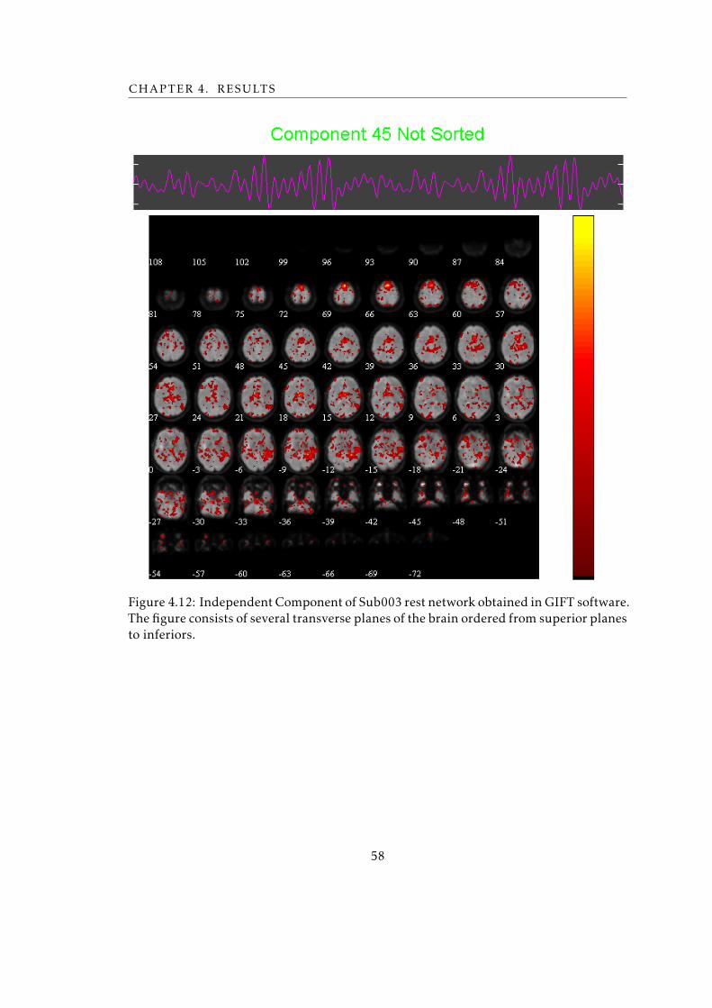
CHAPTER 4. RESULTS
Figure 4.12: Independent Component of Sub003 rest network obtained in GIFT software.The figure consists of several transverse planes of the brain ordered from superior planesto inferiors.
58

4.2. INTRA-SUBJECT ANALYSIS
Table 4.7: Similarity results for rest activation maps and syntactic decision paradigmactivation maps for Sub003
ICIntensity
ThresholdDSC
(max)IC
IntensityThreshold
SC1(max)
ICIntensity
ThresholdSC2
(min)
FWE0.01
6 0.7 0.0347 45 0.1 0.4847 6 0.8 0.86676 0.8 0.0297 36 0.1 0.3593 6 0.7 0.94386 0.6 0.0294 16 0.1 0.3566 6 0.6 0.9737
45 0.2 0.0197 7 0.1 0.2813 26 0.5 0.986345 0.3 0.0190 45 0.2 0.2786 6 0.5 0.9888
FWE0.05
45 0.2 0.0360 45 0.1 0.4219 6 0.8 0.800045 0.3 0.0348 36 0.1 0.3326 6 0.7 0.925039 0.1 0.0287 16 0.1 0.3187 26 0.5 0.958945 0.1 0.0282 45 0.2 0.2452 26 0.6 0.961516 0.2 0.0280 35 0.1 0.2323 6 0.6 0.9650
FWE0.1
45 0.2 0.0439 45 0.1 0.3998 6 0.8 0.80045 0.3 0.0410 16 0.1 0.3057 6 0.7 0.925016 0.3 0.0384 36 0.1 0.2917 6 0.6 0.958416 0.2 0.0368 35 0.1 0.2283 26 0.5 0.958445 0.1 0.0365 45 0.2 0.2218 26 0.6 0.9615
UNC0.001
45 0.1 0.1327 45 0.1 0.3216 23 0.9 0.500045 0.2 0.1219 36 0.1 0.2693 26 0.8 0.500016 0.1 0.1199 16 0.1 0.2595 26 0.9 0.500019 0.1 0.1179 23 0.1 0.2595 27 0.9 0.500036 0.1 0.1170 3 0.1 0.2586 23 0.8 0.5676
59

CHAPTER 4. RESULTS
4.2.2.3 Verb Generation
The results of applying different statistical thresholds to the verb generation data is
represented in the figure 4.13.
From the image is possible to find a robust activation upon sagittal plane immedi-
ately above the corpus callosum. For less restrictive p-values, the superior temporal
gyrus appears activated immediately beneath the Sylvian fissure in both hemispheres.
a FWE p<0.01 b FWE p<0.05
c p<0.1 d p<0.001
Figure 4.13: Independent Component of Sub003 rest network obtained in GIFT software.The figure consists of several transverse planes of the brain ordered from superior planesto inferiors.
The independent component that best overlaps the verb generation map is repre-
sented in figure 4.14. It is possible to verify a large laterality of activations for the left
hemisphere along all planes.
60
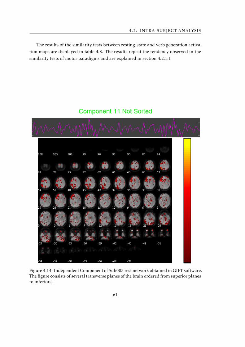
4.2. INTRA-SUBJECT ANALYSIS
The results of the similarity tests between resting-state and verb generation activa-
tion maps are displayed in table 4.8. The results repeat the tendency observed in the
similarity tests of motor paradigms and are explained in section 4.2.1.1
Figure 4.14: Independent Component of Sub003 rest network obtained in GIFT software.The figure consists of several transverse planes of the brain ordered from superior planesto inferiors.
61

CHAPTER 4. RESULTS
Table 4.8: Similarity test results for rest activation maps and verb generation paradigmactivation maps for Sub003
ICIntensity
ThresholdDSC
(max)IC
IntensityThreshold
SC1(max)
ICIntensity
ThresholdSC2
(min)
FWE0.01
11 0.3 0.0451 11 0.1 0.5787 11 0.3 0.972011 0.2 0.0451 6 0.1 0.4676 11 0.2 0.975411 0.4 0.0340 45 0.1 0.4074 6 0.8 0.977811 0.1 0.0253 33 0.1 0.3796 11 0.4 0.973233 0.3 0.0226 35 0.1 0.3796 11 0.5 0.9803
FWE0.05
11 0.2 0.0658 11 0.1 0.5247 6 0.8 0.933311 0.3 0.0573 6 0.1 0.4231 11 0.3 0.959711 0.4 0.0407 45 0.1 0.4121 11 0.4 0.959811 0.1 0.0380 33 0.1 0.3709 11 0.2 0.96218 0.2 0.0357 16 0.1 0.3681 11 0.5 0.9137
FWE0.1
11 0.2 0.0747 11 0.1 0.5126 6 0.8 0.911111 0.3 0.0663 6 0.1 0.4345 11 0.3 0.950711 0.1 0.0441 45 0.1 0.4207 11 0.4 0.95448 0.2 0.0423 35 0.1 0.3701 11 0.2 0.9559
11 0.4 0.0421 16 0.1 0.3655 11 0.5 0.9671
UNC0.001
11 0.2 0.1359 11 0.1 0.4086 6 0.8 0.666711 0.1 0.1086 45 0.1 0.3837 6 0.9 0.714311 0.3 0.0909 6 0.1 0.3830 6 0.7 0.850039 0.1 0.0768 35 0.1 0.3439 11 0.4 0.87408 0.2 0.0720 16 0.1 0.3419 11 0.3 0.8791
4.2.2.4 Multi-language task
Similarly to motor tasks, an overlay map of the three linguistic tasks was created and
compared with the resting state map. The results of that test are displayed in table
4.9. The displayed pattern repeats the individual tendency of each task, which is, Dice
Similarity Coefficient (DSC) has the lowest correlation values among the 3 similarity
coefficients, whereas the Similarity Coefficient 2 has the highest outcomes. The simi-
larity values of DSC increase for p-values less conservative, while SC1 and SC2values
decrease.
62

4.2. INTRA-SUBJECT ANALYSIS
Table 4.9: Similarity test results for rest activation maps and with the result of thesuperposition of the 3 motor tasks for Sub003
ICIntensity
ThresholdDSC
(max)IC
IntensityThreshold
SC1(max)
ICIntensity
ThresholdSC2
(min)
FWE0.01
11 0.2 0.0405 45 0.1 0.4520 6 0.8 0.866711 0.3 0.0344 16 0.1 0.3594 6 0.7 0.943811 0.1 0.0301 36 0.1 0.3025 11 0.3 0.972039 0.1 0.0298 35 0.1 0.2900 11 0.4 0.973245 0.2 0.0263 6 0.1 0.2829 6 0.6 0.9737
FWE0.05
11 0.2 0.0542 45 0.1 0.4114 8 0.9 0.000039 0.1 0.0459 16 0.1 0.3351 8 0.8 0.666745 0.2 0.0456 36 0.1 0.2870 8 0.7 0.727311 0.1 0.0453 35 0.1 0.2752 6 0.8 0.800045 0.3 0.0419 6 0.1 0.2407 8 0.6 0.9000
FWE0.1
11 0.2 0.0574 45 0.1 0.4008 8 0.9 0.000045 0.2 0.0554 16 0.1 0.3194 8 0.7 0.545511 0.1 0.0546 36 0.1 0.2695 8 0.8 0.666739 0.1 0.0519 35 0.1 0.2688 8 0.6 0.800045 0.3 0.0508 6 0.1 0.2421 6 0.8 0.8000
UNC0.001
45 0.1 0.1552 45 0.1 0.3275 8 0.8 0.000016 0.1 0.1408 16 0.1 0.2756 8 0.9 0.000045 0.2 0.1360 35 0.1 0.2695 8 0.7 0.090937 0.1 0.1328 36 0.1 0.2639 8 0.6 0.400011 0.1 0.1325 3 0.1 0.2620 26 0.9 0.5000
63
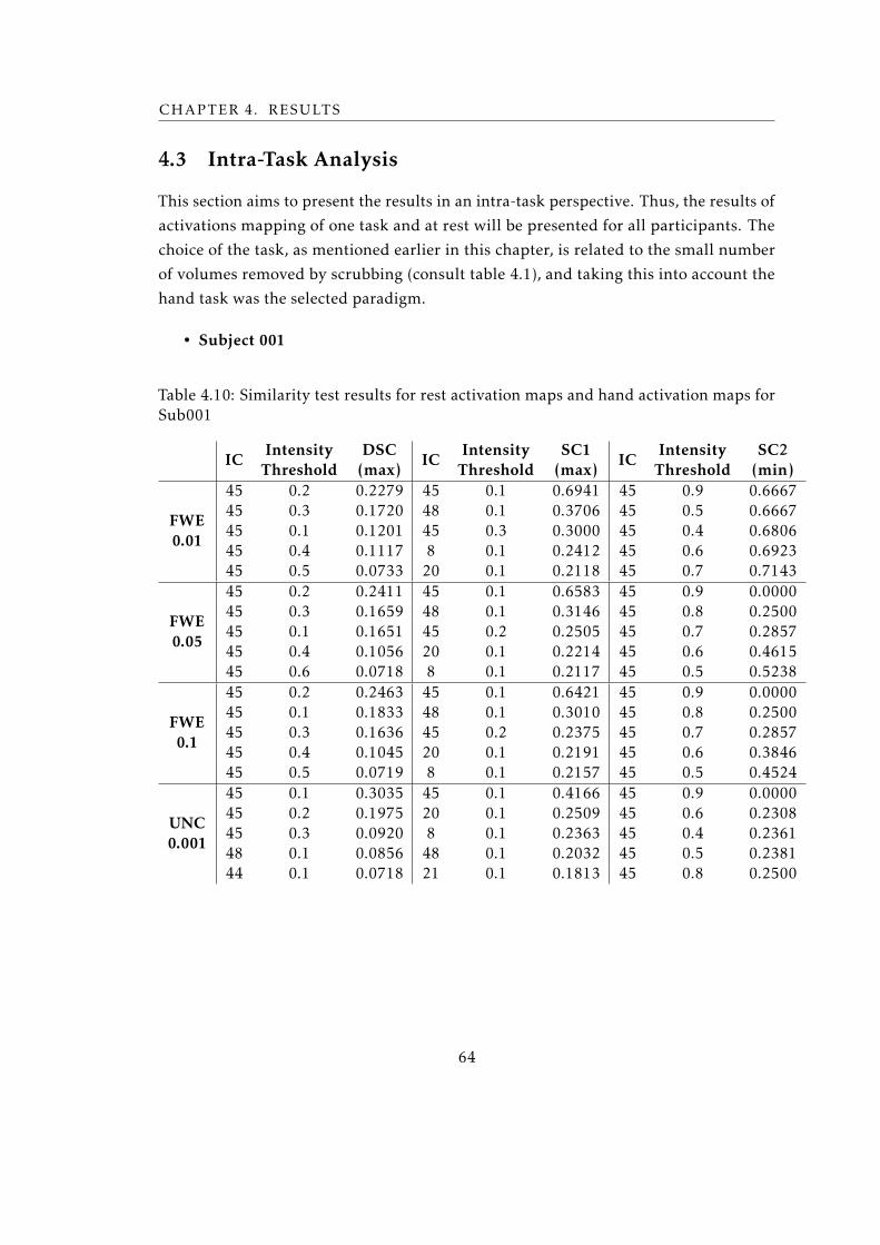
CHAPTER 4. RESULTS
4.3 Intra-Task Analysis
This section aims to present the results in an intra-task perspective. Thus, the results of
activations mapping of one task and at rest will be presented for all participants. The
choice of the task, as mentioned earlier in this chapter, is related to the small number
of volumes removed by scrubbing (consult table 4.1), and taking this into account the
hand task was the selected paradigm.
• Subject 001
Table 4.10: Similarity test results for rest activation maps and hand activation maps forSub001
ICIntensity
ThresholdDSC
(max)IC
IntensityThreshold
SC1(max)
ICIntensity
ThresholdSC2
(min)
FWE0.01
45 0.2 0.2279 45 0.1 0.6941 45 0.9 0.666745 0.3 0.1720 48 0.1 0.3706 45 0.5 0.666745 0.1 0.1201 45 0.3 0.3000 45 0.4 0.680645 0.4 0.1117 8 0.1 0.2412 45 0.6 0.692345 0.5 0.0733 20 0.1 0.2118 45 0.7 0.7143
FWE0.05
45 0.2 0.2411 45 0.1 0.6583 45 0.9 0.000045 0.3 0.1659 48 0.1 0.3146 45 0.8 0.250045 0.1 0.1651 45 0.2 0.2505 45 0.7 0.285745 0.4 0.1056 20 0.1 0.2214 45 0.6 0.461545 0.6 0.0718 8 0.1 0.2117 45 0.5 0.5238
FWE0.1
45 0.2 0.2463 45 0.1 0.6421 45 0.9 0.000045 0.1 0.1833 48 0.1 0.3010 45 0.8 0.250045 0.3 0.1636 45 0.2 0.2375 45 0.7 0.285745 0.4 0.1045 20 0.1 0.2191 45 0.6 0.384645 0.5 0.0719 8 0.1 0.2157 45 0.5 0.4524
UNC0.001
45 0.1 0.3035 45 0.1 0.4166 45 0.9 0.000045 0.2 0.1975 20 0.1 0.2509 45 0.6 0.230845 0.3 0.0920 8 0.1 0.2363 45 0.4 0.236148 0.1 0.0856 48 0.1 0.2032 45 0.5 0.238144 0.1 0.0718 21 0.1 0.1813 45 0.8 0.2500
64
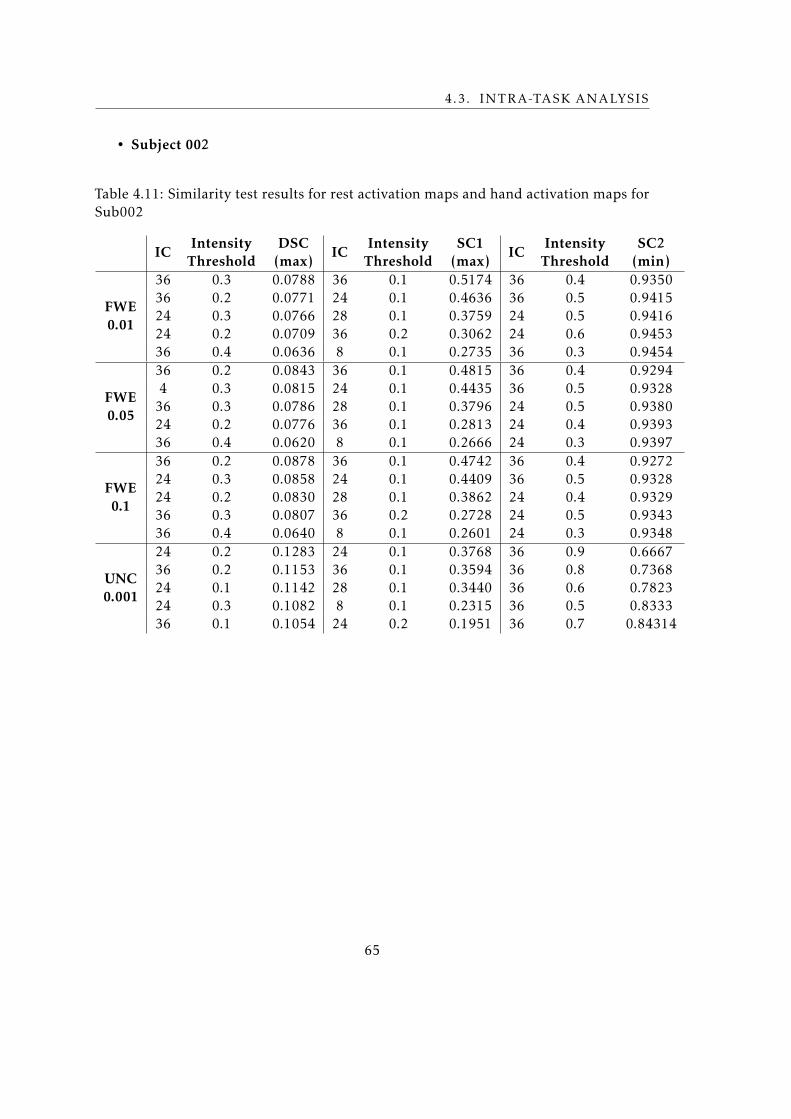
4.3. INTRA-TASK ANALYSIS
• Subject 002
Table 4.11: Similarity test results for rest activation maps and hand activation maps forSub002
ICIntensity
ThresholdDSC
(max)IC
IntensityThreshold
SC1(max)
ICIntensity
ThresholdSC2
(min)
FWE0.01
36 0.3 0.0788 36 0.1 0.5174 36 0.4 0.935036 0.2 0.0771 24 0.1 0.4636 36 0.5 0.941524 0.3 0.0766 28 0.1 0.3759 24 0.5 0.941624 0.2 0.0709 36 0.2 0.3062 24 0.6 0.945336 0.4 0.0636 8 0.1 0.2735 36 0.3 0.9454
FWE0.05
36 0.2 0.0843 36 0.1 0.4815 36 0.4 0.92944 0.3 0.0815 24 0.1 0.4435 36 0.5 0.9328
36 0.3 0.0786 28 0.1 0.3796 24 0.5 0.938024 0.2 0.0776 36 0.1 0.2813 24 0.4 0.939336 0.4 0.0620 8 0.1 0.2666 24 0.3 0.9397
FWE0.1
36 0.2 0.0878 36 0.1 0.4742 36 0.4 0.927224 0.3 0.0858 24 0.1 0.4409 36 0.5 0.932824 0.2 0.0830 28 0.1 0.3862 24 0.4 0.932936 0.3 0.0807 36 0.2 0.2728 24 0.5 0.934336 0.4 0.0640 8 0.1 0.2601 24 0.3 0.9348
UNC0.001
24 0.2 0.1283 24 0.1 0.3768 36 0.9 0.666736 0.2 0.1153 36 0.1 0.3594 36 0.8 0.736824 0.1 0.1142 28 0.1 0.3440 36 0.6 0.782324 0.3 0.1082 8 0.1 0.2315 36 0.5 0.833336 0.1 0.1054 24 0.2 0.1951 36 0.7 0.84314
65
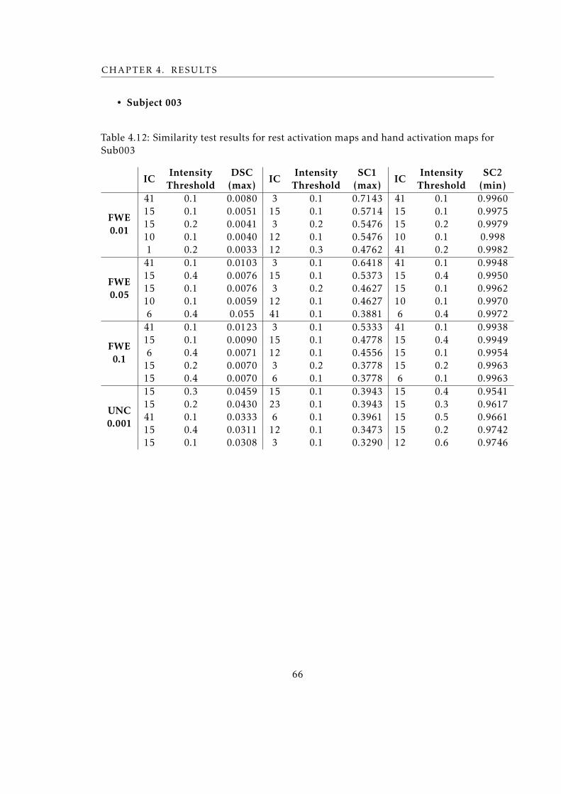
CHAPTER 4. RESULTS
• Subject 003
Table 4.12: Similarity test results for rest activation maps and hand activation maps forSub003
ICIntensity
ThresholdDSC
(max)IC
IntensityThreshold
SC1(max)
ICIntensity
ThresholdSC2
(min)
FWE0.01
41 0.1 0.0080 3 0.1 0.7143 41 0.1 0.996015 0.1 0.0051 15 0.1 0.5714 15 0.1 0.997515 0.2 0.0041 3 0.2 0.5476 15 0.2 0.997910 0.1 0.0040 12 0.1 0.5476 10 0.1 0.9981 0.2 0.0033 12 0.3 0.4762 41 0.2 0.9982
FWE0.05
41 0.1 0.0103 3 0.1 0.6418 41 0.1 0.994815 0.4 0.0076 15 0.1 0.5373 15 0.4 0.995015 0.1 0.0076 3 0.2 0.4627 15 0.1 0.996210 0.1 0.0059 12 0.1 0.4627 10 0.1 0.99706 0.4 0.055 41 0.1 0.3881 6 0.4 0.9972
FWE0.1
41 0.1 0.0123 3 0.1 0.5333 41 0.1 0.993815 0.1 0.0090 15 0.1 0.4778 15 0.4 0.99496 0.4 0.0071 12 0.1 0.4556 15 0.1 0.9954
15 0.2 0.0070 3 0.2 0.3778 15 0.2 0.996315 0.4 0.0070 6 0.1 0.3778 6 0.1 0.9963
UNC0.001
15 0.3 0.0459 15 0.1 0.3943 15 0.4 0.954115 0.2 0.0430 23 0.1 0.3943 15 0.3 0.961741 0.1 0.0333 6 0.1 0.3961 15 0.5 0.966115 0.4 0.0311 12 0.1 0.3473 15 0.2 0.974215 0.1 0.0308 3 0.1 0.3290 12 0.6 0.9746
66

4.3. INTRA-TASK ANALYSIS
• Subject 004
Table 4.13: Similarity test results for rest activation maps and hand activation maps forSub004
ICIntensity
ThresholdDSC
(max)IC
IntensityThreshold
SC1(max)
ICIntensity
ThresholdSC2
(max)
FWE0.01
46 0.1 0.0370 2 0.1 0.2712 46 0.1 0.979727 0.1 0.0340 50 0.1 0.2522 50 0.3 0.980550 0.2 0.0311 40 0.1 0.2366 50 0.4 0.981115 0.1 0.0305 46 0.1 0.2106 27 0.1 0.981350 0.1 0.0297 27 0.1 0.1932 50 0.2 0.9819
FWE0.05
46 0.1 0.0426 50 0.1 0.2732 50 0.4 0.968950 0.2 0.0426 2 0.1 0.2496 50 0.5 0.969527 0.1 0.0406 40 0.1 0.2382 50 0.3 0.970050 0.3 0.0403 46 0.1 0.2039 50 0.2 0.974650 0.1 0.0385 44 0.1 0.1946 50 0.6 0.9748
FWE0.1
50 0.2 0.0487 50 0.1 0.2846 50 0.4 0.963946 0.1 0.0479 40 0.1 0.2421 50 0.5 0.965950 0.1 0.0441 2 0.1 0.2389 50 0.6 0.966450 0.3 0.0430 46 0.1 0.2086 50 0.3 0.966927 0.1 0.0428 44 0.1 0.2022 40 0.5 0.9674
UNC0.001
50 0.2 0.0939 50 0.1 0.3121 50 0.5 0.906650 0.1 0.0920 40 0.1 0.2303 50 0.4 0.911546 0.1 0.0825 44 0.1 0.2122 50 0.6 0.911850 0.3 0.0739 46 0.1 0.1962 50 0.3 0.922044 0.1 0.0682 2 0.1 0.1811 40 0.6 0.9316
67
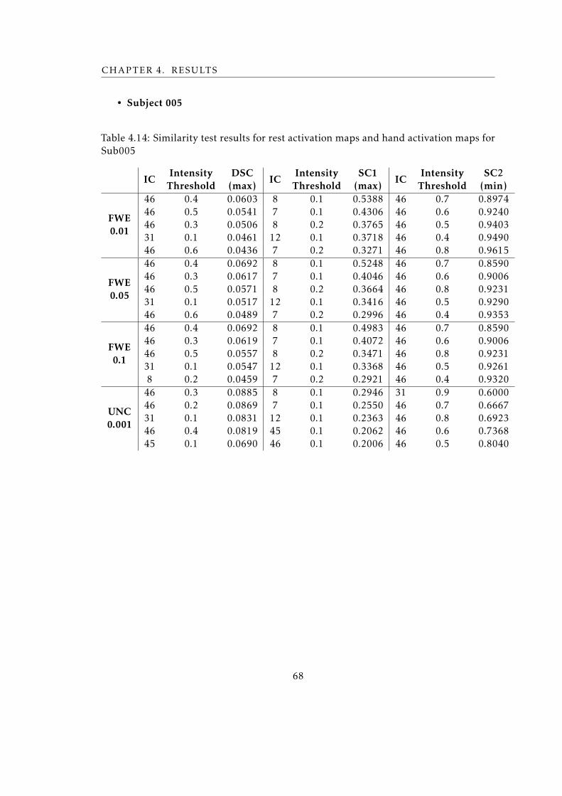
CHAPTER 4. RESULTS
• Subject 005
Table 4.14: Similarity test results for rest activation maps and hand activation maps forSub005
ICIntensity
ThresholdDSC
(max)IC
IntensityThreshold
SC1(max)
ICIntensity
ThresholdSC2
(min)
FWE0.01
46 0.4 0.0603 8 0.1 0.5388 46 0.7 0.897446 0.5 0.0541 7 0.1 0.4306 46 0.6 0.924046 0.3 0.0506 8 0.2 0.3765 46 0.5 0.940331 0.1 0.0461 12 0.1 0.3718 46 0.4 0.949046 0.6 0.0436 7 0.2 0.3271 46 0.8 0.9615
FWE0.05
46 0.4 0.0692 8 0.1 0.5248 46 0.7 0.859046 0.3 0.0617 7 0.1 0.4046 46 0.6 0.900646 0.5 0.0571 8 0.2 0.3664 46 0.8 0.923131 0.1 0.0517 12 0.1 0.3416 46 0.5 0.929046 0.6 0.0489 7 0.2 0.2996 46 0.4 0.9353
FWE0.1
46 0.4 0.0692 8 0.1 0.4983 46 0.7 0.859046 0.3 0.0619 7 0.1 0.4072 46 0.6 0.900646 0.5 0.0557 8 0.2 0.3471 46 0.8 0.923131 0.1 0.0547 12 0.1 0.3368 46 0.5 0.92618 0.2 0.0459 7 0.2 0.2921 46 0.4 0.9320
UNC0.001
46 0.3 0.0885 8 0.1 0.2946 31 0.9 0.600046 0.2 0.0869 7 0.1 0.2550 46 0.7 0.666731 0.1 0.0831 12 0.1 0.2363 46 0.8 0.692346 0.4 0.0819 45 0.1 0.2062 46 0.6 0.736845 0.1 0.0690 46 0.1 0.2006 46 0.5 0.8040
68

4.3. INTRA-TASK ANALYSIS
• Subject 006
Table 4.15: Similarity test results for rest activation maps and hand activation maps forSub006
ICIntensity
ThresholdDSC
(max)IC
IntensityThreshold
SC1(max)
ICIntensity
ThresholdSC2
(max)
FWE0.01
44 0.1 0.0076 6 0.1 0.3684 14 0.5 0.995440 0.3 0.0071 44 0.1 0.3211 44 0.1 0.996240 0.2 0.0069 40 0.1 0.2737 40 0.3 0.996240 0.1 0.0059 6 0.2 0.2105 40 0.2 0.996514 0.5 0.0049 30 0.1 0.2053 40 0.1 0.9970
FWE0.05
44 0.1 0.0117 6 0.1 0.3709 44 0.1 0.994040 0.1 0.0095 44 0.1 0.3146 14 0.4 0.994840 0.2 0.0091 40 0.1 0.2781 40 0.1 0.995230 0.1 0.0078 30 0.1 0.2351 40 0.2 0.995340 0.3 0.0075 6 0.1 0.2318 14 0.5 0.9954
FWE0.1
44 0.1 0.0138 6 0.1 0.3714 14 0.4 0.992240 0.1 0.0111 44 0.1 0.3200 44 0.1 0.993040 0.2 0.0108 40 0.1 0.2829 44 0.4 0.993440 0.3 0.0092 6 0.2 0.2257 14 0.3 0.993714 0.3 0.0087 30 0.1 0.2171 40 0.1 0.9943
UNC0.001
40 0.3 0.0426 6 0.1 0.3529 41 0.8 0.888940 0.2 0.0426 40 0.1 0.3417 41 0.6 0.888940 0.1 0.0397 44 0.1 0.2998 43 0.7 0.909144 0.1 0.0379 6 0.2 0.2142 41 0.7 0.913040 0.4 0.0317 30 0.1 0.1993 5 0.6 0.9167
69
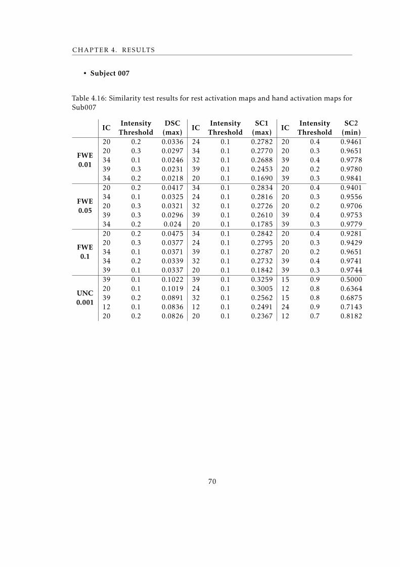
CHAPTER 4. RESULTS
• Subject 007
Table 4.16: Similarity test results for rest activation maps and hand activation maps forSub007
ICIntensity
ThresholdDSC
(max)IC
IntensityThreshold
SC1(max)
ICIntensity
ThresholdSC2
(min)
FWE0.01
20 0.2 0.0336 24 0.1 0.2782 20 0.4 0.946120 0.3 0.0297 34 0.1 0.2770 20 0.3 0.965134 0.1 0.0246 32 0.1 0.2688 39 0.4 0.977839 0.3 0.0231 39 0.1 0.2453 20 0.2 0.978034 0.2 0.0218 20 0.1 0.1690 39 0.3 0.9841
FWE0.05
20 0.2 0.0417 34 0.1 0.2834 20 0.4 0.940134 0.1 0.0325 24 0.1 0.2816 20 0.3 0.955620 0.3 0.0321 32 0.1 0.2726 20 0.2 0.970639 0.3 0.0296 39 0.1 0.2610 39 0.4 0.975334 0.2 0.024 20 0.1 0.1785 39 0.3 0.9779
FWE0.1
20 0.2 0.0475 34 0.1 0.2842 20 0.4 0.928120 0.3 0.0377 24 0.1 0.2795 20 0.3 0.942934 0.1 0.0371 39 0.1 0.2787 20 0.2 0.965134 0.2 0.0339 32 0.1 0.2732 39 0.4 0.974139 0.1 0.0337 20 0.1 0.1842 39 0.3 0.9744
UNC0.001
39 0.1 0.1022 39 0.1 0.3259 15 0.9 0.500020 0.1 0.1019 24 0.1 0.3005 12 0.8 0.636439 0.2 0.0891 32 0.1 0.2562 15 0.8 0.687512 0.1 0.0836 12 0.1 0.2491 24 0.9 0.714320 0.2 0.0826 20 0.1 0.2367 12 0.7 0.8182
70

4.3. INTRA-TASK ANALYSIS
• Subject 008
Table 4.17: Similarity test results for rest activation maps and hand activation maps forSub008
ICIntensity
ThresholdDSC
(max)IC
IntensityThreshold
SC1(max)
ICIntensity
ThresholdSC2
(min)
FWE0.01
19 0.1 0.1204 19 0.1 0.4092 19 0.9 0.000019 0.2 0.1151 31 0.1 0.3598 19 0.8 0.444419 0.3 0.1053 2 0.1 0.3233 19 0.7 0.655219 0.4 0.0773 9 0.1 0.2412 19 0.6 0.69329 0.1 0.0732 45 0.1 0.1850 19 0.5 0.7317
FWE0.05
19 0.1 0.1633 19 0.1 0.4021 19 0.9 0.000019 0.2 0.1445 31 0.1 0.3306 19 0.8 0.444419 0.3 0.1176 2 0.1 0.2935 19 0.7 0.51729 0.1 0.1000 9 0.1 0.2393 19 0.6 0.60239 0.2 0.0929 45 0.1 0.1855 19 0.5 0.6146
FWE0.1
19 0.1 0.1840 19 0.1 0.3934 19 0.9 0.000019 0.2 0.1545 31 0.1 0.3215 19 0.8 0.111119 0.3 0.1197 2 0.1 0.2835 19 0.7 0.37939 0.1 0.1141 9 0.1 0.2373 19 0.6 0.5114
31 0.1 0.1010 21 0.1 0.1924 19 0.5 0.5561
UNC0.001
19 0.1 0.3220 19 0.1 0.3097 19 0.9 0.000031 0.1 0.2348 31 0.1 0.2949 19 0.7 0.06909 0.1 0.2310 2 0.1 0.2355 19 0.8 0.11116 0.1 0.2146 6 0.1 0.2311 10 0.7 0.1304
45 0.1 0.2097 9 0.1 0.2184 19 0.6 0.1364
The task under analysis has a low similarity to rest data of the respective subject.
The maximum DSC was approximately 30.35% for the subject001 and the maximum
value of SC1 was 71.43% for the subject 003.The subject with the most satisfactory
coefficients is the Sub008, with DSC = 12%, SC1 = 40.92%, and finally a SC2 = 0%. On
the other hand, the subject with less satisfactory coefficients was the subject 006 with
DSC = 0.76%, SC1= 36.84% and SC2 = 99.54%.
71
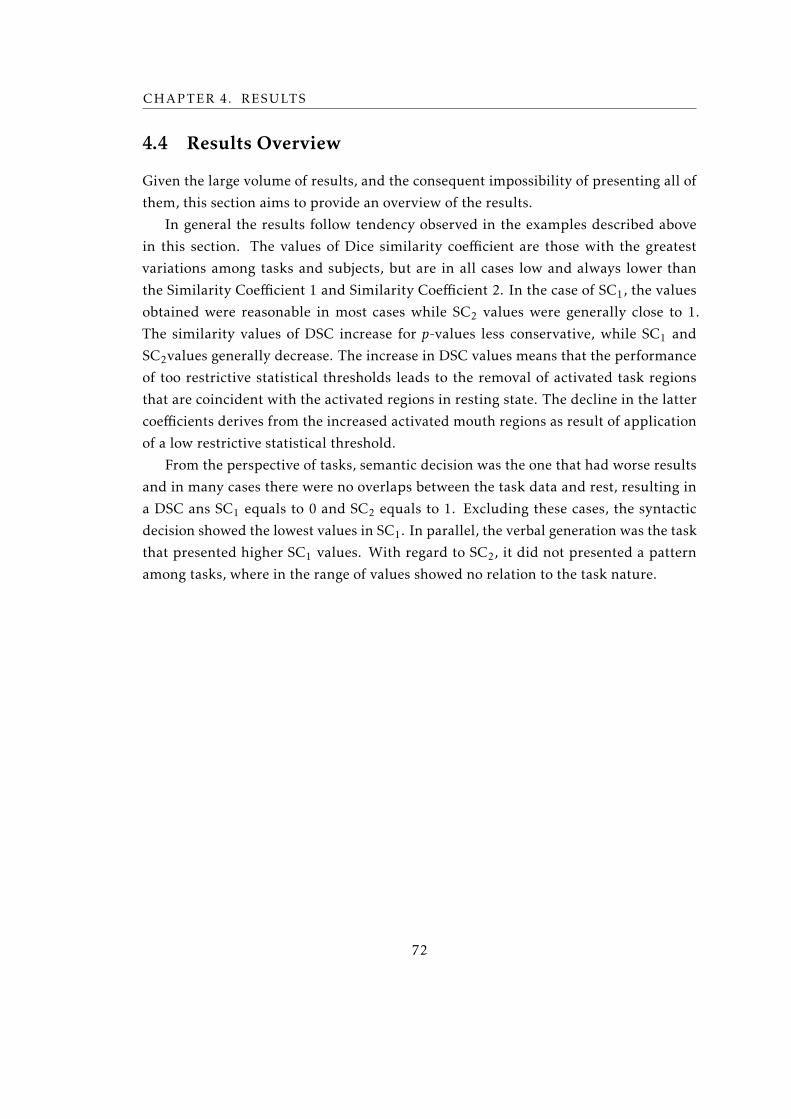
CHAPTER 4. RESULTS
4.4 Results Overview
Given the large volume of results, and the consequent impossibility of presenting all of
them, this section aims to provide an overview of the results.
In general the results follow tendency observed in the examples described above
in this section. The values of Dice similarity coefficient are those with the greatest
variations among tasks and subjects, but are in all cases low and always lower than
the Similarity Coefficient 1 and Similarity Coefficient 2. In the case of SC1, the values
obtained were reasonable in most cases while SC2 values were generally close to 1.
The similarity values of DSC increase for p-values less conservative, while SC1 and
SC2values generally decrease. The increase in DSC values means that the performance
of too restrictive statistical thresholds leads to the removal of activated task regions
that are coincident with the activated regions in resting state. The decline in the latter
coefficients derives from the increased activated mouth regions as result of application
of a low restrictive statistical threshold.
From the perspective of tasks, semantic decision was the one that had worse results
and in many cases there were no overlaps between the task data and rest, resulting in
a DSC ans SC1 equals to 0 and SC2 equals to 1. Excluding these cases, the syntactic
decision showed the lowest values in SC1. In parallel, the verbal generation was the task
that presented higher SC1 values. With regard to SC2, it did not presented a pattern
among tasks, where in the range of values showed no relation to the task nature.
72

Chapter
5Discussion
The task-free nature of rs-fMRI has propelled many studies of brain connectivity. Efforts
are being made to translate these studies into clinical practice. In this study, we explored
the feasibility of resting-state fMRI as a complement to task-based fMRI for presurgical
planning.
In order to accomplish the goal of this study, we first explored all preprocessing
parameters and conceived the most efficient protocol.
To correct the effects of head movement in the BOLD signal in task-based fMRI
we refer to scrubbing and 6 realignment parameters regression. We noticed a greater
impact of scrubbing on linguistic tasks. The origin of this trend may be related to two
factors coming from the architecture of these paradigms. The first is the high frequency
of the stimulus occurrence, and the second is the response requirements. The demand
for a quick response can lead to unintentional micro-movements. Semantic decision was
the task that had a higher number of scrubbed volumes, and hence the one that involved
a greater head movement. Among motor tasks, feet movement was the one that induced
the greatest amount of volumes scrubbed, followed by mouth and hand movement. In
the first case the translation in the z-axis and rotation in the y-axis implied by foot
motion induces movement over the whole body, thereby causing head displacements.
As regards to the mouth task, it entails the movement of the jaw causing undesired
head movements. Finally, hand paradigms was the task that causes less displacements
because of the limited motor exigency of the task.
73
CHAPTER 5. DISCUSSION
In resting-state fMRI we established two approaches, the first was to repeat the
procedure used in task and the second was to additionally remove intrinsic signals to
the brain - nuisance covariates removal. We followed the protocol used by Yan et al.
(2013) [55], which regressed out WM and CSF, however adding further global signal
regressor, an approach taken by Satterthwaite et al. (2013) [57]. However, countering
to these studies, we realized that this latter led to results that were visually worse and
had a more pronounced effect in the extraction of independent components, resulting
in poorer outcomes in the analysis of similarity with task data. The source of these
worse results can arise from the processing protocol chosen by us. A possible reintro-
duction of artefacts into the RS-fcMRI time series could be avoided by the simultaneous
performance of nuisance signals regression and filtering, as proposed by Hallquist et
al. (2013) [58]. Notwithstanding, the performance of any two processes simultaneously
was unattainable due to the particularities of the used software (DPARSFA).
In this study we have also found a strong relationship between the age of participants
and the number of volumes removed by scrubbing. In our sample, the younger subjects
were those who performed the largest number of displacements per task. These results
are consistent with previous studies (Power et al.(2012), Satterthwaite et al., (2012) and
Yan et al. [56] [57] [55]). The study carried out by Power demonstrated how scrubbing
may change fundamental conclusions about patterns of functional connectivity. This
can be particularly critical in rest data, since the efficiency of resting-state networks
extraction is result of a good separation of independent components. In our study, a
large decrease of volumes has not meant a visually different spatial distribution of the
regions activated. Although, the application of a less strict framewise displacement
threshold, such as FD > 0.7 mm, could improve the similarity analysis results.
Another preprocessing step that can be the source of introducing artifacts is nor-
malization. Brain normalization is important for individual subjects, and not only for
inter-subject data, since it allows to establish relations between regions activated from
the rest and task maps maps when the fields of view of rest and task acquisitions do
not match. Despite the need of its application, there is no guarantee that there were no
misaligned structures between different paradigms, which consequently may result in
false negative and positive activations.
As regards to task data processing, most of the results are visually concordant with
the expectations from the literature and clinical practice. A subset of the data was
assessed by an experienced neurologist who confirmed the consistency of the results.
74

However, the observed variations may be due not only to the spikes in BOLD signal
from the micro-movements of the head, but also to a natural adjustment of the brain.
The plasticity of the brain is an important variable to take into account in the study
of functional and resting state networks, especially in pre-surgical planning. In these
cases, it is especially crucial to choose a good set of statistical thresholds. In this study
we explore the influence of the application of 4 distinct p-values (0.01 FWE; 0.05 FWE;
0.1 FWE and 0.001 UNC). For more stringent thresholds, important activated regions
were no longer visible, or the extent of activation was not fully covered. In contrast,
when p-values were more lenient, false positive activations emerged. It is therefore
impossible to draw any conclusion about what the best threshold is.Rather, information
stemming from several , p-values should be taken into consideration during the process
and will result in an informed analysis about the location and extent of the areas to be
avoided in surgical resection. This assumption has a direct impact on the calculation
of the similarity between the task and rest data. Low statistical thresholds authenticate
the specificity of the overlap, yet imply low sensitivity. On the other hand, sensitivity
increases for higher p-values, thereby not guaranteeing specific results.
To process the resting-state data, our approach was to replicate the procedures per-
formed in several previous studies involving the same software (GIFT). Therefore, we
generated ICA maps for 20 and 50 independent components, following a rough ap-
proach of Sair et al. (2015) [42]. As they reported, the similarity analysis improved
with increasing the number of extracted components. Accordingly, we performed inde-
pendent component analysis resorting to 50 IC in order to obtain the best concordance
with task maps. Even so, there was no evident observable similarity between the inde-
pendent components extracted for each participant with the well-known default mode
networks. Despite the impossibility of choosing an ideal number of independent com-
ponents highlighted by Hui et al. (2011), the number of components to be extracted
is crucial, since for a low number of IC, different brain networks may merge, while for
higher numbers there is a risk of splitting a relevant network into several ICs. Another
reason for the discrepancy between the areas activated at rest and the expected default
mode networks can result from the choice of the algorithm that tests the stability and
reliability of independent components, such as its amount of runs. Because of the scarce
information found in the literature, the chosen algorithm was the one that was used in
similar studies (ICASSO). As regards to the number of times that the algorithm runs,
we opted for a relatively low number (compared with the number mentioned in Tie et
al.(2014) [44]) because of the high computation time that the procedure requires. The
application of another algorithm and a greater number of runs could potentially lead
75
CHAPTER 5. DISCUSSION
to extracting resting state networks more resembling to task networks.
Finally, we performed three analysis of similarity between the rest maps and the
map of each of the six tasks for every subject.
The first coefficient, Dice Similarity Coefficient, was previously used in several other
studies, including Sair et al. (2015) [42] and Branco et al. (2016) [43]. In the scope of
this study, this index can be referred as an appraiser of the specificity of the overlay
map. The results obtained are found to be unsatisfactory and in the case of language
tasks the outcomes are much lower than those obtained in the studies aforementioned.
To investigate why these values were low, we conducted two additional tests, which we
call SC1 and SC2. The former is a sensitivity test while the second intended to find the
contribution of rest activations in the overlap of the two maps. As the results obtained in
SC1 were quite higher than in DSC we can say that the number of undetected activations
is restricted. This conclusion is highly relevant in the context of brain portions resection,
since the removal of eloquent areas must be minimized: sensitivity more important than
specificity in this context, because a false negative means that a relevant activated area
went undetected and may end up removed by resection. Therefore we may conclude
that the poor results of the DSC come from an excessive number of activated regions
in resting-state, which if confirmed by the high levels of SC2. This result confirms the
need to extract independent components more fragmented (i.e. increase the number of
IC), in order to improve the specificity of the results.
76

Chapter
6Conclusion
The present study was carried out in the context of the current interest in understanding
the usefulness of resting state networks in the clinical environment. This study aimed
to assess the feasibility of using the resting state networks as a complementary approach
to the classical procedure that resorts to task-based mapping of brain regions whose
resection should be avoided in brain tumor surgery. The selected approach was to mea-
sure the similarity between the activation maps at rest of a subject with the activation
maps of each task to the same subject.
With this goal in mind, a pre-processing protocol was devised and tested in order
to obtain images which provide an optimal extraction of activation networks. The
resulting images were then processed. The approaches conducted for processing rest
and task images were different and were adapted from those already reported in the
literature. The resemblance of these maps was subsequently evaluated using several
similarity coefficients.
The obtained results allowed to conclude that the selected methodology is remark-
ably sensitive to activated regions detection and its extension. However a reduced
specificity is found which results from an inefficient detection of common activations
at rest and task. Nonetheless, even though low specificity restricts the application of rs-
fMRI as a exclusive method of mapping important regions of the brain, high sensitivity
shows that resting state fMRI could become a complementary method to the task-based
classic approach in the future.
77

CHAPTER 6. CONCLUSION
In order for rs-fMRI to be widely used as a complement to task-based fMRI, further
studies will be required to improve these results. Some pre-processing and processing
procedures may be reevaluated, namely those that contradict what is described in the
literature. A refinement of the procedure for rest network detection, including opti-
mization for single-subject analysis as opposed to groups, is also contemplated in order
to improve the specificity of the method. Another interesting approach would also be to
reproduce this study to other clinical cases referred for surgical resection of portions of
the brain, such as epilepsy, in order to understand how the different disorders may affect
communication in the brain at rest and consequently assess how is that hypothetical
change could lead to a greater resemblance to the regions activated by task.
It should be stressed that this thesis was carried out as part of an ongoing project
that involves collaboration with clinical partners. Several refinements, including the
ones mentioned above, are expected to be implemented in this context, and thereby to
bring about an improved performance of the protocols that are currently in place in a
clinical setting
78

Bibliography
[1] M. K. Sidhu, J. Stretton, G. P. Winston, A. W. McEvoy, M. Symms, P. J. Thompson,
M. J. Koepp, and J. S. Duncan, “Memory network plasticity after temporal lobe
resection : a longitudinal functional imaging study”, Brain, vol. 139, no. Pt 2,
pp. 1–16, 2016.
[2] F. Pittau, P. Mégevand, L. Sheybani, E. Abela, F. Grouiller, L. Spinelli, C. M.
Michel, M. Seeck, and S. Vulliemoz, “Mapping epileptic activity : sources or
networks for the clinicians ?”, Frontiers in Neurology, vol. 5, no. 1, pp. 1–21, 2014.
[3] D. Zhang, J. M. Johnston, M. D. Fox, C Eric, R. L. Grubb, M. R. Chicoine, M. D.
Smyth, A. Z. Snyder, M. E. Raichle, and J. S. Shimony, “Preoperative Sensorimotor
Mapping in Brain Tumor Patients using Spontaneous Fluctuations in Neuronal
Activity Imaged with fMRI: Initial Experience”, Neurosurgery, vol. 65, no. 314,
pp. 226–236, 2010.
[4] G. Spena, A. Nava, F. Cassini, A. Pepoli, M. Bruno, F. D’Agata, F. Cauda, K. Sacco, S.
Duca, L. Barletta, and P. Versari, “Preoperative and intraoperative brain mapping
for the resection of eloquent-area tumors. A prospective analysis of methodology,
correlation, and usefulness based on clinical outcomes”, Acta Neurochirurgica, vol.
152, no. 11, pp. 1835–1845, 2010.
[5] K. E. Weaver, W. A. Chaovalitwongse, E. J. Novotny, A Poliakov, T. G. Grabowski,
and J. G. Ojemann, “Local functional connectivity as a pre-surgical tool for seizure
focus identification in non-lesion, focal epilepsy”, Frontiers in Neurology, vol. 4,
no. 43, pp. 1–14, 2013.
[6] C. Rosazza, D. Aquino, L. D’Incerti, R. Cordella, A. Andronache, D. Zacà, M. G.
Bruzzone, G. Tringali, and L. Minati, “Preoperative mapping of the sensorimotor
cortex: Comparative assessment of task-based and resting-state fMRI”, PLoS ONE,
vol. 9, no. 6, pp. 1–19, 2014.
79
BIBLIOGRAPHY
[7] M. P. van den Heuvel and H. E. Hulshoff Pol, “Exploring the brain network: A
review on resting-state fMRI functional connectivity”, European Neuropsychophar-macology, vol. 20, no. 8, pp. 519–534, 2010.
[8] M. D. Fox and M Greicius, “Clinical applications of resting state functional con-
nectivity”, Frontiers in systems neuroscience, vol. 4, no. June, pp. 1–137, 2010.
[9] M. F. Bear, B. W. Connors, and M. A. Paradiso, “The Structure of the Nervous Sys-
tem”, in Neuroscience - Exploring the brain, E. Lupash, Ed., 3rd Edition, Baltimore:
Lippincott Williams & Wilkins, 2006, ch. Chapter 7, pp. 168 –204.
[10] V. Stark-Vance and M. L. Dubay, “The basics”, in 100 Questions & answers aboutbrain tumors, Sudbury, Massachusetts: Jones & Bartlett Learning, 2010, ch. 1st
Chapte, pp. 1–4, isbn: 1449630995.
[11] R. T. Merrell, “Brain Tumors”, Disease-a-Month, vol. 58, no. 12, pp. 678–689,
2012.
[12] H. Marsh, “Brain tumours”, Surgery (Oxford), vol. 27, no. 3, pp. 135–138, 2009.
[13] What You Need To Know About Brain Tumors. 2009, pp. 1–51.
[14] D. Glass-Macenka, “Understanding brain tumors.”, in Frankly Speaking aboutcancer, T. J. Hopkins, Ed., 2008, pp. 5–14.
[15] D. A. Hardesty and P. Nakaji, “The Current and Future Treatment of Brain Metas-
tases”, Frontiers in Surgery, vol. 3, no. May, pp. 1–7, 2016.
[16] J. M. González, “Management of Brain Tumors in Eloquent Areas”, in DiagnosticTechniques and Surgical Management Of Brain Tumors, A. L. Abujamra, Ed., 3rd
Edition, Rijeka, Croatia: InTech, 2011, ch. 25, pp. 168 –204.
[17] M. G. Allen, A. Z. Snyder, C. D. Hacker, T. J. Mitchell, E. C. Leuthardt, and
J. S. Shimony, “Task-Based Presurgical Functional MRI in Patients with Brain
Tumors”, in Clinical Functional MRI: Presurgical Functional Neuroimaging, A. B. B.
Leuven, M. K. Göttingen, and K. S. Heidelberg, Eds., Berlin: Springer, 2007, ch. 4,
pp. 143–158.
[18] M. Ragnehed, “Clinical application of functional MRI.”, in Functional magneticresonance imaging for clinical diagnosis- exploring and improving the examinationchain, 1121, vol. 34, Linköping: Elsevier, 2009, ch. 4, pp. 267–277.
[19] S. Borchers, M. Himmelbach, N. Logothetis, and H.-O. Karnath, “Direct electrical
stimulation of human cortex - the gold standard for mapping brain functions?”,
Nature reviews. Neuroscience, vol. 13, no. 1, pp. 63–70, 2012.
80

BIBLIOGRAPHY
[20] M. J. Hamberger and J. Cole, “Language organization and reorganization in
epilepsy”, Neuropsychology Review, vol. 21, no. 3, pp. 240–251, 2011.
[21] M. F. Hartshorne, “Positron emission tomography”, in Functional Brain Imaging,
vol. 187, St. Louis: Elsevier Health Sciences, 1995, ch. 5, pp. 187–212.
[22] J. Brito, “Dynamic Functional Connectivity of BOLD fMRI signal during both rest
and task execution states Dynamic Functional Connectivity of BOLD fMRI signal
during both rest and task execution states”, Master’s thesis, 2014, pp. 1–2.
[23] E. W. Pang and O. C. Snead III, “From Structure to Circuits: The Contribution
of MEG Connectivity Studies to Functional Neurosurgery”, Frontiers in Neu-roanatomy, vol. 10, no. June, pp. 1–14, 2016.
[24] C. G. Roth, “Introduction to Body MRI”, in Fundamentals of Body MRI, 3, vol. 264,
Elsevier Health Sciences, 2012, ch. 1, pp. 1–34.
[25] K. Uludag, D. J. Dubowitz, and R. B. Buxton, “Clinical magnetic resonance imag-
ing”, in Clinical MRI. Elsevier, San Diego, R. R. Edelman, J. Hesselink, and M.
Zlatkin, Eds., 3rd Editio, Philadelphia: Saunders Elsevier, 2006, ch. 9, pp. 249–
287.
[26] M. Ragnehed, “Funtcitonal MRI”, in Functional Magnetic Resonance imaging forclinical diagnosis - exploring and improving the examination chain, 1121, Sweden:
LiU-tryck, 2009, ch. 3.
[27] J. C. Gore, “Principles and practice of functional MRI of the human brain”, Journalof Clinical Investigation, vol. 112, no. 1, pp. 4–9, 2003.
[28] H Mao and G. S. Berns, “MRI in the study of brain functions : clinical perspec-
tives”, MedicaMundi, vol. 46, no. 1, pp. 28–38, 2002.
[29] S. Yorkwilliams and K. L. Poston, “What light have resting state fMRI studies shed
on cognition and mood in Parkinson ’ s disease ?”, Journal of Clinical MovementDisorders, vol. 1, no. 1, pp. 1–12, 2014.
[30] S. Li, A. Eloyan, S. Joel, S. Mostofsky, J. Pekar, S. S. Bassett, and B. Caffo, “Analysis
of Group ICA-Based Connectivity Measures from fMRI: Application to Alzheimer’s
Disease”, PLoS ONE, vol. 7, no. 11, pp. 1–10, 2012.
[31] A. Z. Snyder and M. E. Raichle, “A Brief History of the Resting State: the Wash-
ington University Perspective”, NeuroImage, vol. 62, no. 2, pp. 902–910, 2012.
81
BIBLIOGRAPHY
[32] S. S. Kety and C. F. Schmidt, “The nitrous oxide method for the quantative deter-
mination of cerebral blood flow in man: theory, procedure and normal values”,
The Journal of clinical investigation, vol. 27, no. 4, pp. 476–483, 1948.
[33] P. L. Purdon and R. M. Weisskoff, “Effect of temporal autocorrelation due to
physiological noise and stimulus paradigm on voxel-level false-positive rates in
fMRI”, Human Brain Mapping, vol. 6, no. 4, pp. 239–249, 1998.
[34] K. J. Friston, S Williams, R Howard, R. S. Frackowiak, and R Turner, “Movement-
related effects in fMRI time-series”, Magnetic resonance in medicine, vol. 35, no. 3,
pp. 346–355, 1996.
[35] B. B. Biswal, “Resting state fMRI: A personal history”, in NeuroImage, 2, vol. 62,
Elsevier Inc., 2012, pp. 938–944.
[36] D. Cordes, V. M. Haughton, K. Arfanakis, G. J. Wendt, P. A. Turski, C. H. Moritz,
M. A. Quigley, and M. E. Meyerand, “Mapping functionally related regionsof
brain with functional connectivity MR imaging”, American Society of Neuroradiol-ogy, vol. 21, no. 9, pp. 1636–1644, 2000.
[37] R. L. Buckner, J. R. Andrews-Hanna, and D. L. Schacter, “The Brain’s Default
Network”, Annals of the New York Academy of Sciences, vol. 1124, no. 1, pp. 1–38,
2008.
[38] L. Heine, A. Soddu, F. Gómez, A. Vanhaudenhuyse, L. Tshibanda, M. Thonnard,
V. Charland-Verville, M. Kirsch, S. Laureys, and A. Demertzi, “Resting state net-
works and consciousness Alterations of multiple resting state network connec-
tivity in physiological, pharmacological, and pathological consciousness states”,
Frontiers in Psychology, vol. 3, no. August, pp. 1–12, 2012.
[39] J. C. Tamraz and Y. G. Comair, “Central Region and Motor Cortex”, in Atlas ofRegional Anatomy of the Brain Using MRI, 2005, ch. 4, pp. 51–116.
[40] M. H. Lee, C. D. Smyser, and J. S. Shimony, “Resting state fMRI: A review of
methods and clinical applications”, American Journal of Neuroradiology, vol. 34,
no. 10, pp. 1866–1872, 2013.
[41] Radiology Key. [Online]. Available: http://radiologykey.com/magnetic-
resonance-imaging-2/ (visited on 08/01/2016).
82

BIBLIOGRAPHY
[42] H. I. Sair, N. Yahyavi-Firouz-Abadi, V. D. Calhoun, R. D. Airan, S. Agarwal, J.
Intrapiromkul, A. S. Choe, S. K. Gujar, B. Caffo, M. A. Lindquist, and J. J. Pillai,
“Presurgical brain mapping of the language network in patients with brain tumors
using resting-state fMRI: Comparison with task fMRI”, Human Brain Mapping,
vol. 37, no. 3, pp. 913–923, 2016.
[43] P. Branco, D. Seixas, S. Deprez, S. Kovacs, R. Peeters, S. L. Castro, and S. Sunaert,
“Resting-State Functional Magnetic Resonance Imaging for Language Preopera-
tive Planning”, Frontiers in human neuroscience, vol. 10, no. February, pp. 1–14,
2016.
[44] Y. Tie, L. Rigolo, I. H. Norton, R. Y. Huang, W. Wu, D. Orringer, S. Mukundan,
and A. J. Golby, “Defining language networks from resting-state fMRI for surgical
planning- A feasibility study”, Human Brain Mapping, vol. 35, no. 3, pp. 1018–
1030, 2014.
[45] C. M. Bennett, G. L. Wolford, and M. B. Miller, “The principled control of false
positives in neuroimaging”, Social Cognitive and Affective Neuroscience, vol. 4, no.
4, pp. 417–422, 2009.
[46] J. R. Andrews-Hanna, A. Z. Snyder, J. L. Vincent, C. Lustig, D. Head, M. E. Raichle,
and R. L. Buckner, “Disruption of large-scale brain systems in advanced aging”,
Neuron, vol. 56, no. 5, pp. 924–935, 2007.
[47] M. D. Iglesia-vaya, J. Molina-mateo, M. J. Escarti-fabra, A. S. Kanaan, and L. Martí-
bonmatí, “Brain Connections – Resting State fMRI Functional Connectivity”, in
Novel Frontiers of Advanced Neuroimaging, K. N. Fountas, Ed., 2013, ch. 3, pp. 51–
66.
[48] Y. Golland, P. Golland, S. Bentin, and R. Malach, “Data-driven clustering reveals
a fundamental subdivision of the human cortex into two global systems”, Neu-ropsychologia, vol. 46, no. 2, pp. 540–553, 2008.
[49] M. H. Lee, C. D. Hacker, A. Z. Snyder, M. Corbetta, D. Zhang, E. C. Leuthardt,
and J. S. Shimony, “Clustering of resting state networks”, PLoS ONE, vol. 7, no.
7, pp. 1–12, 2012.
[50] S. M. H. N. Suma, “Principal Component Analysis for Analysis and Classification
of fMRI Activation Maps”, Journal of Computer Science and network security, vol. 7,
no. 11, pp. 235–242, 2007.
83

BIBLIOGRAPHY
[51] K. Friston, C. Frith, P. Liddle, and R. Frackowiak, “Functional Connectivity : The
Principal-Component Analysis of Large ( PET ) Data Sets”, Journal of CerebralBlood Flow & Metabolism, vol. 13, no. 1, pp. 5–14, 1993.
[52] J. Damoiseaux, S. Rombouts, F Barkhof, P Scheltens, C. Stam, S. M. Smith, and
C. Beckmann, “Consistent resting-state networks across healthy subjects”, Pro-ceedings of the national academy of sciences, vol. 103, no. 37, pp. 13 848–13 853,
2006.
[53] V. Kiviniemi, J.-H. Kantola, J. Jauhiainen, A. Hyvärinen, and O. Tervonen, “Inde-
pendent component analysis of nondeterministic fMRI signal sources”, vol. 19,
no. 2, pp. 253–260, 2003.
[54] C. F. Beckmann, M. Deluca, J. T. Devlin, S. M. Smith, J. R. Hospital, and O. Ox,
“Investigations into resting-state connectivity using independent component anal-
ysis”, no. May, pp. 1001–1013, 2005.
[55] C. G. Yan, B Cheung, C Kelly, S Colcombe, R. C. Craddock, A Di Martino, Q Li,
X. N. Zuo, F. X. Castellanos, and M. P. Milham, “A comprehensive assessment of
regional variation in the impact of micromovement head motion on functional
connectomics”, Neuroimage, vol. 76, pp. 183–201, 2013.
[56] J. D. Power, K. A. Barnes, A. Z. Snyder, B. L. Schlaggar, and S. E. Petersen, “Spu-
rious but systematic correlations in functional connectivity MRI networks arise
from subject motion”, NeuroImage, vol. 59, no. 3, pp. 2142–2154, 2012.
[57] T. D. Satterthwaite, D. H. Wolf, J. Loughead, K. Ruparel, M. A. Elliott, H. Hakonar-
son, R. C. Gur, and R. E. Gur, “Impact of in-scanner head motion on multiple
measures of functional connectivity: Relevance for studies of neurodevelopment
in youth”, NeuroImage, vol. 60, no. 1, pp. 623–632, 2012.
[58] M. N. Hallquist, K. Hwang, and B. Luna, “The nuisance of nuisance regression:
Spectral misspecification in a common approach to resting-state fmri preprocess-
ing reintroduces noise and obscures functional connectivity”, Neuroimage, vol. 82,
pp. 208–225, 2013.
84