Embed Size (px)
Citation preview

http://dx.doi.org/10.1590/0104-1428.1621
SSSSSSSSSSSSSSSSSSSS
Polímeros, 25(3), 277-288, 2015 277
Analysis of equations of state for polymersErlí José Padilha Júnior1, Rafael de Pelegrini Soares1 and Nilo Sérgio Medeiros Cardozo1*
1Departamento de Engenharia Química – DEQUI, Universidade do Rio Grande do Sul – UFRGS, Porto Alegre, RS, Brazil
Sbstract
In the literature there are several studies comparing the accuracy of various models in describing the PvT behavior of polymers. However, most of these studies do not provide information about the quality of the estimated parameters or the sensitivity of the prediction of thermodynamic properties to the parameters of the equations. Furthermore, there are few studies exploring the prediction of thermal expansion and compression coefficients. Based on these observations, the objective of this study is to deepen the analysis of Tait, HH (Hartmann-Haque), MCM (modified cell model) and SHT (simplified hole theory) equations of state in predicting the PvT behavior of polymers, for both molten and solid states. The results showed that all equations of state provide an adequate description of the PvT behavior in the molten state, with low standard deviations in the estimation of parameters, adequate sensitivity of their parameters and plausible prediction of specific volume, thermal expansion and isothermal compression coefficients. In the solid state the Tait equation exhibited similar performance to the molten state, while HH showed satisfactory results for amorphous polymers and difficulty in adjusting the PvT curve for semicrystalline polymers.
Keywords: equation of state, PvT behavior, polymer.
1. Introduction
The study of the thermodynamic behavior of polymers is essential to analyze the physical transformations that occur during processing, e.g. injection molding or extrusion, and to predict the properties of the final products. Polymers in melt state or in solution can be represented correctly by an equation of state (EoS) because these can be considered equilibrium states for polymers. Conversely, the solid state is at least one quasi-equilibrium state, because the properties depend on the conditions of solidification, as the cooling rate and pressure, which difficults their description by means of EoS[1].
Numerous equations of state have been developed to describe the PvT (pressure-volume-temperature) behavior of polymers. In literature, there are several studies comparing the fitting accuracy of various models for PvT data of polymers[1-7]. These studies are focused mainly in the analysis of the fitting accuracy of the specific volume in the molten state, employing usually the method of least squares[2,3,6,8-20] for the parameter estimation step. They showed that the theoretical equations based on cell-and-hole models and the Tait and the Hartmann-Haque (HH) empirical equations are those which provide more accurate fitting of the experimental data.
On the other hand, little information is available in the literature on at least two important aspects that are essential for the use of the referred equations in process simulation: quality of the estimated parameters as a function of the model employed and fitting accuracy of the models for thermal expansion and isothermal compression coefficients.
The isobaric thermal expansion coefficient ( β ) and isothermal compressibility ( κ ) are defined by:
1 PT
∂ν β= ν ∂ (1)
1 TP
∂ν κ=− ν ∂ (2)
where the negative sign indicates the volume decrease with pressure increase[21].
These coefficients are important for the simulation of polymer processing operations, because they are present in the governing equation of energy conservation. However, to the best of our knowledge, the only studies on their prediction from EoS are those of Utracki[22,23], in which the prediction of thermal expansivity and compressibility by hole models is analyzed.
Based on these observations, the objective of this study is to deepen the analysis of Tait, HH, MCM (modified cell model) and SHT (simplified hole theory) equations of state in prediction of PvT behavior of polymers, in both molten and solid physical states. The EoS were analyzed with respect to: (i) quality in the estimation of its parameters by the method of least squares, (ii) sensitivity of their predictions to each of its parameters, (iii) quality of the prediction of the specific volume, and (iv) quality of the prediction of isobaric thermal expansion coefficient and isothermal compressibility.
2. Equations of State Analyzed
2.1 Tait equation of state
This equation is purely empirical, and was originally proposed for water. Presently, through various modifications, it is applied to a wide variety of substances, being possibly one of the equations of state most used to model the PvT behavior of polymers[3]. For some authors, it is not a true equation of state, but an isothermal compressibility model

Padilha, E. J., Jr., Soares, R. P., & Cardozo, N. S. M.
Polímeros , 25(3), 277-288, 2015278
(i.e., a volume-pressure relationship). Tait equation can be written as[3]:
( ) ( ) ( ) ( ), 1 1 ,o tPv T P v T Cln v T P
B T
= − + +
(3)
where for polymers in the molten state, i.e., above the liquid-solid transition temperature:
( )1 2 5 o m mv b b T b= + − (4a)
( ) ( )3 4 5expm mB T b b T b = − − (4b)
( ), 0t T Pν = (4c)
and for polymers in solid state, i.e., below the liquid-solid transition temperature
( )1 2 5 o s sv b b T b= + − (5a)
( ) ( )3 4 5exps sB T b b T b = − − (5b)
( ) ( ) ( ){ }7 8 5 9,t T P b exp b T b b P ν = − − (5c)
The liquid-solid transition temperature, which is the glass transition temperature for amorphous polymers and the melting or crystallization temperature for semicrystalline polymers, can be calculated by
( ) 5 6tT P b b P= + (6)
In these equations, v is the specific volume of the polymeric material; the coefficient C is a constant equal to 0.0894; ov is the specific volume at zero pressure; tν is the specific volume corresponding to crystalline phase; B is the sensitivity to pressure of material; 1b at 9b are parameters of model, obtained by fitting of PvT diagram. The parameters 1mb to 4mb and 1sb to 4sb describe the dependence on pressure and temperature in the molten and the solid state, respectively; 5b and 6b are parameters that describe the change of transition temperature with pressure;
7b to 9 b are particular parameters of semicrystalline polymers that describe the form of the state transition[24].
2.2 HH equation of state
Hartmann and Haque[10] developed an empirical equation of state combining the thermal pressure function of Pastine and Warfield, the zero-pressure isobar presented by Somcynsky and Simha, and the empirical dependence of volume with the thermal pressure. HH EoS describes the PvT behavior of polymers in the molten and solid states. It is given by:
5 3/2Pv T lnv= −
(7)
where the dimensionless variables P , v and T for molten polymers are defined as:
0 0 0 ; ;
m m m
P v TP v TB v T
= = =
(8)
and for solid polymers as:
0 0 0 ; ;
s s s
P v TP v TB v T
= = =
(9)
where 0B , 0v and 0T are the characteristic parameters. 0T and 0v are defined as temperature and specific volume,
respectively, extrapolated to zero pressure, while 0B is identified as the isothermal bulk modulus extrapolated to zero temperature and pressure.
2.3 MCM equation of state
The modified cell model equation of state was developed by Dee and Walsh[2], starting from the formalism presented by Prigogine et al.[25]. In the cell model, the compressibility and thermal expansion of the structure are explained only by changes in the cell volume. Dee and Walsh[2] introduced a numerical factor that scales the hard-core cell volume in the free volume term, disconnecting the theory from the specific geometry. This factor, q , was found to be constant for numerous polymers and equal to about 1.07. MCM EoS can be written as:
1/3
1/3 2 42 1.2045 1.011 –
– 0.8909Pv vT Tv q v v
= −
(10)
The reduced parameters P , v and T are defined as:
* * * ; ; P v TP v TP v T
= = = (11)
where *P , *v and *T are characteristic parameters.
2.4 SHT equation of state
The hole theory introduces empty cells in the cell model[26], based on the concept that the thermal expansion of liquid is mainly due to holes ( h ), i.e., the empty cells, while volume changes of the cells are also allowed. Zhong et al.[27] simplified the hole theory through the use of an exponential function to the fraction of occupied cells. SHT EoS is derived as:
( )( ) ( ) ( )
1/3
1/3 2 22 1.1394 –1 .5317
– 0.9165
yvPv yT yv y T yv yv
= +
(12)
where P , v and T are reduced parameters defined by Equation 11, y is the fraction of occupied cells, being defined by:
0.52/1 Ty e−= − (13)
3. Methodology
The experimental PvT data used in this work were taken from the literature[7,21,28-32] as shown in Table 1. For each polymer, the available data were subdivided in two sets: one used for parameter estimation (DATA1) and other for validation (DATA2). The construction of these subsets was based on random selection of points.
Differently from specific volume data, the isobaric thermal expansion and isothermal compression coefficients are hard to obtain experimentally. Thus, the EoS were only qualitatively analyzed with relation to the prediction of these

Analysis of equations of state for polymers
Polímeros, 25(3), 277-288, 2015 279
Tabl
e 1.
Rel
evan
t inf
orm
atio
n ab
out t
he e
xper
imen
tal P
vT d
ata
used
a .
Poly
mer
Am
orph
ous
Sem
icry
stal
line
PSPC
PMM
APC
HM
APn
BMA
PoM
SiP
PLP
EPE
OPA
6PL
APB
S-B
Ref
eren
ce28
2930
3030
3129
327
2132
32
Pres
sure
rang
e (M
Pa)
0.1-
200
0.1-
200
0.1-
180
0.1-
180
0.1-
180
0.1-
180
0.1-
200
0.1-
200
0.1-
200
0.1-
190
0.1-
200
0.1-
200
Tem
pera
ture
rang
e (K
)28
0-46
831
3-60
335
3-42
335
7-45
328
5-35
530
2-47
031
3-57
331
3-49
331
3-49
336
4-58
631
3-49
331
3-49
3
Initi
al te
mpe
ratu
re o
f an
alys
is (K
)46
831
335
335
728
530
231
331
331
336
431
331
3
Initi
al p
ress
ure
of
anal
ysis
(MPa
)0.
10.
10.
10.
10.
10.
10.
10.
10.
10.
10.
10.
1
Num
ber o
f exp
erim
enta
l po
ints
in so
lid st
ate
used
fo
r par
amet
er e
stim
atio
n
3326
3630
2925
2841
2735
5616
Num
ber o
f exp
erim
enta
l po
ints
in m
olte
n st
ate
used
for p
aram
eter
es
timat
ion
2830
2026
2226
2529
4317
2120
Num
ber o
f exp
erim
enta
l po
ints
in so
lid st
ate
used
fo
r the
ana
lysis
of t
he
pred
ictio
n ac
cura
cy
3324
-30
--
28-
-35
-15
Num
ber o
f exp
erim
enta
l po
ints
in m
olte
n st
ate
used
for t
he a
naly
sis o
f th
e pr
edic
tion
accu
racy
2832
-26
--
24-
-17
-19
Expe
rimen
tal d
ata
varia
nce
(2 ex
pσ
)
0.00
030.
001
0.00
040.
0004
0.00
040.
0004
0.00
10.
002
0.00
20.
0003
0.00
20.
002
a Dat
a ob
tain
ed b
y th
e m
etho
d of
con
finin
g flu
id in
isot
herm
al m
ode,
exc
ept f
or p
olys
tyre
ne, f
or w
hich
the
expe
rimen
ts w
ere
cond
ucte
d in
isob
aric
mod
.

Padilha, E. J., Jr., Soares, R. P., & Cardozo, N. S. M.
Polímeros , 25(3), 277-288, 2015280
coefficients, taking as basis of comparison their theoretically expected behavior. The estimation of parameters was conducted by the least squares method, using the lsqnonlin function already implemented in MatLab software, with the following objective function ( FObj ):
( )21
ˆn
i ii
FObj v v=
= −∑ (14)
where ( )i iv v− is the residual between predicted ( iv ) and experimental ( iv ) values and n is the number of points considered.
The parameters of the equations of state were estimated simultaneously, as suggested by Hartmann and Haque[10]. For the Tait EoS, firstly, 5b and 6b were estimated from data of transition temperature at different pressures. The melt parameters ( 1mb , 2mb , 3mb and 4mb ) and solid parameters ( 1sb , 2sb , 3sb , 4sb , 7b , 8b and 9b ) were estimated separately from data corresponding to the respective states[33]. Likewise, for HH EoS, the experimental data were divided into two states: molten and solid state. The parameters of the MCM and SHT EoS were estimated only with molten state data.
The quality of the estimated parameters for each model was analyzed in terms of their covariance matrix ( Vα ), evaluated using a routine developed in MatLab, according the following expression[34]:
( )1 2 1 TTyV H G G H− −
α α α α α= σ (15)
where 2yσ is the experimental data variance, Hα is the
Hessian matrix of FObj , and Gα is the matrix that represents the derivative of the gradient of FObj with relation to the experimental values iv .
The normalized parameter sensitivity matrix was used to evaluate the sensitivity of the predictions of the considered EoS to parameter variations. The coefficients of this matrix are given by:
* ˆˆ
jiij
j i
avSa v
∂= ∂
(16)
where ja is the parameter of the equation analyzed. These coefficients were calculated using a MatLab function, according to the following central-difference approximation:
( ) ( )*2
i j i j jij
i
v h v hS
h v
α + − α − α =
(17)
with h equal to 10-4. In this way, the parameter sensitivity of the specific volume predictions was analyzed in a wide temperature range, at different pressures, for polycarbonate and linear polyethylene.
To appraise the fit and prediction quality of each model, the mean relative deviation (MRD) and the regression coefficient ( 2R ) were calculated:
1
0 ˆ1 0 n i i
i i
v vMRD
n v=
−= ∑ (18)
( )( )
212
2 1
ˆ1
ni ii
ni ii
v vR
v v=
=
−∑= −
−∑ (19)
where iv is the arithmetic mean of experimental specific volumes.
Additionally, F-tests were performed to assess the suitability of the considered models. The value of 0F used in the comparison with the critical value of F ( cF = F distribution value corresponding to 95% confidence) was defined as the ratio between the model ( 2
eosσ ) and the experimental ( 2
expσ ) variances, according to the following expression:
( )22
0 2 2
ˆni ii
eos
exp exp
v vn npF
−∑σ −= =σ σ
(20)
where np is the number of estimated parameters. The experimental variances are shown in Table 1.
4. Results and Discussion
4.1 Fitting and prediction of specific volume
As mentioned previously, the comparison of the EoS under analysis with relation to the fitting of specific volume data has already been extensively studied by other authors[2,3,6,8-20]. Therefore, in the present work, the analysis corresponding to the fitting stage will be focused only in the quality of the estimated parameters, aspect for which there is little information available in the literature.
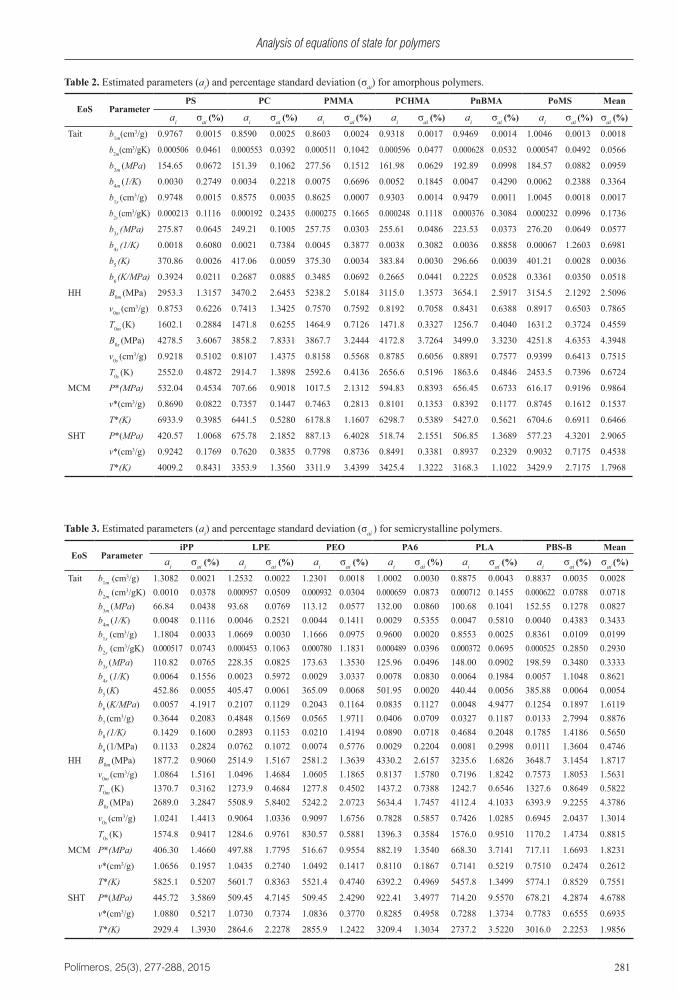
The values of parameters estimated from data set DATA1 and their respective standard deviations are presented in Tables 2 and 3, for the amorphous and semicrystalline polymers, respectively. The low values of the standard deviations indicate that the fitting were adequate. The parameters of equations of state showed a higher standard deviation for semicrystalline polymers, in both physical states. The fitting of Tait and HH EoS were better in molten state, both to amorphous and semicrystalline polymers. In general, Tait equation exhibited the lowest values of standard deviations (below 2%) except for the parameter 6b in the cases of the polymers iPP and PLA, for which the linear dependence between transition temperature and pressure described by Equation 6 is not obeyed. For all equations of state, the greatest deviations were found for the parameters related to pressure, what can be explained by the wide range of pressure analyzed.
For the evaluation of the prediction capability of the studied models, calculations of specific volume for the conditions corresponding to each experimental data of data set DATA2 were performed using the values of parameters estimated with data set DATA1 (Tables 2 and 3). The values of 0F , MRD and 2R obtained are presented in Table 4, together with the respective values of cF used in the F-test to 95% confidence. As can be seen in Table 4, all the four EoS provided predictions not significantly different from the experimental data ( 0F < cF ), showing their adequacy in the prediction of the PvT behavior of the considered polymers. It is observed that Tait equation exhibited the lowest relative deviation module mean and the highest regression coefficient in most cases. However, the other equations of state studied also presented satisfactory results, with values close to those obtained with Tait EoS. The only exception was in the prediction of specific volume of semicrystalline
Analysis of equations of state for polymers
Polímeros, 25(3), 277-288, 2015 281
Table 2. Estimated parameters (ai) and percentage standard deviation (σai) for amorphous polymers.
EoS ParameterPS PC PMMA PCHMA PnBMA PoMS Mean
ai σai (%) ai σai (%) ai σai (%) ai σai (%) ai σai (%) ai σai (%) σai (%)
Tait b1m(cm3/g) 0.9767 0.0015 0.8590 0.0025 0.8603 0.0024 0.9318 0.0017 0.9469 0.0014 1.0046 0.0013 0.0018
b2m(cm3/gK) 0.000506 0.0461 0.000553 0.0392 0.000511 0.1042 0.000596 0.0477 0.000628 0.0532 0.000547 0.0492 0.0566
b3m (MPa) 154.65 0.0672 151.39 0.1062 277.56 0.1512 161.98 0.0629 192.89 0.0998 184.57 0.0882 0.0959
b4m (1/K) 0.0030 0.2749 0.0034 0.2218 0.0075 0.6696 0.0052 0.1845 0.0047 0.4290 0.0062 0.2388 0.3364
b1s (cm3/g) 0.9748 0.0015 0.8575 0.0035 0.8625 0.0007 0.9303 0.0014 0.9479 0.0011 1.0045 0.0018 0.0017
b2s (cm3/gK) 0.000213 0.1116 0.000192 0.2435 0.000275 0.1665 0.000248 0.1118 0.000376 0.3084 0.000232 0.0996 0.1736
b3s (MPa) 275.87 0.0645 249.21 0.1005 257.75 0.0303 255.61 0.0486 223.53 0.0373 276.20 0.0649 0.0577
b4s (1/K) 0.0018 0.6080 0.0021 0.7384 0.0045 0.3877 0.0038 0.3082 0.0036 0.8858 0.00067 1.2603 0.6981
b5 (K) 370.86 0.0026 417.06 0.0059 375.30 0.0034 383.84 0.0030 296.66 0.0039 401.21 0.0028 0.0036
b6 (K/MPa) 0.3924 0.0211 0.2687 0.0885 0.3485 0.0692 0.2665 0.0441 0.2225 0.0528 0.3361 0.0350 0.0518
HH B0m (MPa) 2953.3 1.3157 3470.2 2.6453 5238.2 5.0184 3115.0 1.3573 3654.1 2.5917 3154.5 2.1292 2.5096
v0m (cm3/g) 0.8753 0.6226 0.7413 1.3425 0.7570 0.7592 0.8192 0.7058 0.8431 0.6388 0.8917 0.6503 0.7865
T0m (K) 1602.1 0.2884 1471.8 0.6255 1464.9 0.7126 1471.8 0.3327 1256.7 0.4040 1631.2 0.3724 0.4559
B0s (MPa) 4278.5 3.6067 3858.2 7.8331 3867.7 3.2444 4172.8 3.7264 3499.0 3.3230 4251.8 4.6353 4.3948
v0s (cm3/g) 0.9218 0.5102 0.8107 1.4375 0.8158 0.5568 0.8785 0.6056 0.8891 0.7577 0.9399 0.6413 0.7515
T0s (K) 2552.0 0.4872 2914.7 1.3898 2592.6 0.4136 2656.6 0.5196 1863.6 0.4846 2453.5 0.7396 0.6724
MCM P*(MPa) 532.04 0.4534 707.66 0.9018 1017.5 2.1312 594.83 0.8393 656.45 0.6733 616.17 0.9196 0.9864
v*(cm3/g) 0.8690 0.0822 0.7357 0.1447 0.7463 0.2813 0.8101 0.1353 0.8392 0.1177 0.8745 0.1612 0.1537
T*(K) 6933.9 0.3985 6441.5 0.5280 6178.8 1.1607 6298.7 0.5389 5427.0 0.5621 6704.6 0.6911 0.6466
SHT P*(MPa) 420.57 1.0068 675.78 2.1852 887.13 6.4028 518.74 2.1551 506.85 1.3689 577.23 4.3201 2.9065
v*(cm3/g) 0.9242 0.1769 0.7620 0.3835 0.7798 0.8736 0.8491 0.3381 0.8937 0.2329 0.9032 0.7175 0.4538
T*(K) 4009.2 0.8431 3353.9 1.3560 3311.9 3.4399 3425.4 1.3222 3168.3 1.1022 3429.9 2.7175 1.7968
Table 3. Estimated parameters (ai) and percentage standard deviation (σai ) for semicrystalline polymers.
EoS ParameteriPP LPE PEO PA6 PLA PBS-B Mean
ai σai (%) ai σai (%) ai σai (%) ai σai (%) ai σai (%) ai σai (%) σai (%)
Tait b1m (cm3/g) 1.3082 0.0021 1.2532 0.0022 1.2301 0.0018 1.0002 0.0030 0.8875 0.0043 0.8837 0.0035 0.0028b2m (cm3/gK) 0.0010 0.0378 0.000957 0.0509 0.000932 0.0304 0.000659 0.0873 0.000712 0.1455 0.000622 0.0788 0.0718b3m (MPa) 66.84 0.0438 93.68 0.0769 113.12 0.0577 132.00 0.0860 100.68 0.1041 152.55 0.1278 0.0827b4m (1/K) 0.0048 0.1116 0.0046 0.2521 0.0044 0.1411 0.0029 0.5355 0.0047 0.5810 0.0040 0.4383 0.3433b1s (cm3/g) 1.1804 0.0033 1.0669 0.0030 1.1666 0.0975 0.9600 0.0020 0.8553 0.0025 0.8361 0.0109 0.0199b2s (cm3/gK) 0.000517 0.0743 0.000453 0.1063 0.000780 1.1831 0.000489 0.0396 0.000372 0.0695 0.000525 0.2850 0.2930b3s (MPa) 110.82 0.0765 228.35 0.0825 173.63 1.3530 125.96 0.0496 148.00 0.0902 198.59 0.3480 0.3333b4s (1/K) 0.0064 0.1556 0.0023 0.5972 0.0029 3.0337 0.0078 0.0830 0.0064 0.1984 0.0057 1.1048 0.8621b5 (K) 452.86 0.0055 405.47 0.0061 365.09 0.0068 501.95 0.0020 440.44 0.0056 385.88 0.0064 0.0054b6 (K/MPa) 0.0057 4.1917 0.2107 0.1129 0.2043 0.1164 0.0835 0.1127 0.0048 4.9477 0.1254 0.1897 1.6119b7 (cm3/g) 0.3644 0.2083 0.4848 0.1569 0.0565 1.9711 0.0406 0.0709 0.0327 0.1187 0.0133 2.7994 0.8876b8 (1/K) 0.1429 0.1600 0.2893 0.1153 0.0210 1.4194 0.0890 0.0718 0.4684 0.2048 0.1785 1.4186 0.5650b9 (1/MPa) 0.1133 0.2824 0.0762 0.1072 0.0074 0.5776 0.0029 0.2204 0.0081 0.2998 0.0111 1.3604 0.4746
HH B0m (MPa) 1877.2 0.9060 2514.9 1.5167 2581.2 1.3639 4330.2 2.6157 3235.6 1.6826 3648.7 3.1454 1.8717v0m (cm3/g) 1.0864 1.5161 1.0496 1.4684 1.0605 1.1865 0.8137 1.5780 0.7196 1.8242 0.7573 1.8053 1.5631T0m (K) 1370.7 0.3162 1273.9 0.4684 1277.8 0.4502 1437.2 0.7388 1242.7 0.6546 1327.6 0.8649 0.5822B0s (MPa) 2689.0 3.2847 5508.9 5.8402 5242.2 2.0723 5634.4 1.7457 4112.4 4.1033 6393.9 9.2255 4.3786
v0s (cm3/g) 1.0241 1.4413 0.9064 1.0336 0.9097 1.6756 0.7828 0.5857 0.7426 1.0285 0.6945 2.0437 1.3014
T0s (K) 1574.8 0.9417 1284.6 0.9761 830.57 0.5881 1396.3 0.3584 1576.0 0.9510 1170.2 1.4734 0.8815
MCM P*(MPa) 406.30 1.4660 497.88 1.7795 516.67 0.9554 882.19 1.3540 668.30 3.7141 717.11 1.6693 1.8231
v*(cm3/g) 1.0656 0.1957 1.0435 0.2740 1.0492 0.1417 0.8110 0.1867 0.7141 0.5219 0.7510 0.2474 0.2612
T*(K) 5825.1 0.5207 5601.7 0.8363 5521.4 0.4740 6392.2 0.4969 5457.8 1.3499 5774.1 0.8529 0.7551
SHT P*(MPa) 445.72 3.5869 509.45 4.7145 509.45 2.4290 922.41 3.4977 714.20 9.5570 678.21 4.2874 4.6788
v*(cm3/g) 1.0880 0.5217 1.0730 0.7374 1.0836 0.3770 0.8285 0.4958 0.7288 1.3734 0.7783 0.6555 0.6935
T*(K) 2929.4 1.3930 2864.6 2.2278 2855.9 1.2422 3209.4 1.3034 2737.2 3.5220 3016.0 2.2253 1.9856

Padilha, E. J., Jr., Soares, R. P., & Cardozo, N. S. M.
Polímeros , 25(3), 277-288, 2015282
Tabl
e 4.
Sta
tistic
al re
sults
in sp
ecifi
c vo
lum
e pr
edic
tion
by E
oS.
Poly
mer
Mol
ten
Solid
EoS
F ca
EoS
F cbTa
itH
HM
CM
SHT
Tait
HH
MR
D
(%)
R2F 0
MR
D
(%)
R2F 0
MR
D
(%)
R2F 0
MR
D
(%)
R2
F0
MR
D
(%)
R2F
0M
RD
(%
)R2
F0
PS0.
0394
0.99
978.
38×1
0–40.
0581
0.99
921.
81×1
0–90.
0323
0.99
976.
38×1
0–40.
0520
0.99
950.
0013
1.47
920.
0201
0.99
981.
78×1
0–40.
0294
0.99
944.
22×1
0–41.
4393
PC0.
0723
0.99
944.
84×1
0–40.
1077
0.99
907.
27×1
0–40.
1333
0.99
760.
0018
0.11
410.
9988
9.08
×10–4
1.44
650.
0557
0.99
821.
97×1
0–40.
1395
0.98
770.
0012
1.52
00PC
HM
A0.
0364
0.99
986.
11×1
0–40.
1136
0.99
844.
03×1
0–90.
0808
0.99
920.
0020
0.06
120.
9995
0.00
141.
4984
0.06
390.
9976
0.00
200.
1085
0.99
370.
0049
1.46
20IP
P0.
1028
0.99
960.
0017
0.16
000.
9988
0.00
430.
1320
0.99
910.
0031
0.14
780.
9990
0.00
351.
5200
0.43
000.
9249
0.09
330.
9429
0.86
590.
1532
1.47
92PA
60.
1070
0.99
780.
0129
0.10
100.
9980
0.01
010.
0804
0.99
920.
0040
0.10
590.
9987
0.00
671.
6253
0.19
640.
9920
0.02
970.
6487
0.93
160.
2388
1.42
59PB
S-B
0.04
440.
9998
1.66
×10–4
0.05
830.
9996
2.48
×10–4
0.06
120.
9995
2.75
×10–4
0.07
330.
9994
3.40
×10–4
1.58
910.
0890
0.99
785.
40×1
0–40.
1741
0.98
990.
0021
1.66
89A
mor
phou
s Mea
n-
--
--
--
--
--
--
0.04
660.
9985
-0.
0925
0.99
36-
-Se
mic
ryst
alli
ne
Mea
n-
--
--
--
--
--
--
0.23
850.
9716
-0.
5886
0.92
91-
-
Mea
n0.
0671
0.99
94-
0.09
980.
9988
-0.
0867
0.99
91-
0.09
240.
9992
--
--
--
--
-a D
egre
es o
f fre
edom
use
d: 2
8, 3
2, 2
6, 2
4, 1
7 an
d 19
for P
S, P
C, P
CH
MA
, iPP
, PA
6 an
d PB
S-B
, res
pect
ivel
y; b D
egre
es o
f fre
edom
use
d: 3
3, 2
4, 3
0, 2
8, 3
5 an
d 15
for P
S, P
C, P
CH
MA
, iPP
, PA
6 an
d PB
S-B
, res
pect
ivel
y.

Analysis of equations of state for polymers
Polímeros, 25(3), 277-288, 2015 283
polymers in solid state, where a higher difference between Tait and HH equations occurred.
Figure 1 shows the residual plots for each equation of state. It is possible to observed that the predominately random nature of the errors distributions for both molten and solid state data, with the predictions of the HH EoS
for molten iPP as only relevant exception. These results support the statement of good suitability of the EoS tested.
As example of the general behavior described in the previous paragraph, Figure 2 shows the variation of MRD with the temperature for an amorphous polymer, PC, and with the pressure and temperature for a semicrystalline one, iPP. It can be seen that the HH EoS presented a high relative
Figure 1. Residual plots of specific volume predictions for all EoS tested: (a) Molten and (b) Solid state polymers.

Padilha, E. J., Jr., Soares, R. P., & Cardozo, N. S. M.
Polímeros , 25(3), 277-288, 2015284
deviation in solid state, especially at low pressures near the transition temperature (Figures 2c and 2d).
4.2 Sensitivity analysis
The sensitivity of the prediction of specific volume with relation to each parameter of HH, MCM and SHT EoS is shown in Figure 3. The sensitivity of parameters showed similar behavior for all these EoS, both to amorphous and semicrystalline polymers. Besides the highest sensitivity corresponds to the volume related parameters, the sensitivity to each parameter was nearly constant in the whole ranges of pressure and temperature analyzed.
For the Tait EoS, the behavior of the sensitivity to the parameters was somewhat different, as shown in Figure 4. The sensitivity to the parameters 1b and 2b varied continuous and complementarily with the increase of the temperature (Figures 4b and 4c), with increase of the sensitivity to
1b and decrease of the sensitivity to 2b . Moreover, it is perceived that there was an abrupt change in the sensitivity of the parameters of Tait EoS near the transition temperature of linear polyethylene in the solid state. The sensitivities of parameters 1sb and of term tv ( 7b , 8b and 9b ) of Tait equation were modified near the transition region. It is
found that there is a correlation between the sensitivities to the parameters 1sb and 7b , both related to the specific volume. All parameters of the tv term ( 7b , 8b and 9b ) reveal sensitivity close to the transition regions, stating that they are within linked in modeling this region. Thus, this transition region has fundamental importance for the estimation of the parameters of the Tait EoS.
4.3 Isobaric thermal expansion and isothermal compression coefficients prediction analysis
Figure 5 shows the isobaric thermal expansivity calculated from the PC, PoMS, iPP and PLA by equations of state. It is observed that all the EoS predict similar values of this coefficient and are in qualitative agreement with the theory in the sense that the thermal expansion coefficient of a polymer melt is always greater than that of the corresponding amorphous and semicrystalline solid[35,36]. However, Tait EoS, unlike the other equations, predicts a reduction of this coefficient with the increase of the temperature, contrarily to theoretical expectations[35], revealing a limitation of the model. Moreover, in the case of semicrystalline polymers, Tait equation of state presented an abrupt increase in thermal expansion coefficient in the
Figure 2. MRD (%) in specific volume prediction: (a) PC in 10 MPa, (b) PC in 200 MPa, (c) iPP in 443.8 K and (d) iPP in 20 MPa.

Analysis of equations of state for polymers
Polímeros, 25(3), 277-288, 2015 285
Figure 3. Normalized sensitivity of specific volume relative to the parameters of: (a) HH EoS to PC in 0.1 MPa, (b) HH EoS to LPE in 200 MPa, (c) MCM EoS to PC in 0.1 MPa, (d) MCM EoS to LPE in 200 MPa, (e) SHT EoS to PC in 200 MPa and (f) SHT EoS to LPE in 0.1 MPa.
crystalline transition region. This occurs because Tait EoS describes satisfactorily sudden change in specific volume due to destruction/growth of crystallites, which does not happen with the HH equation. The theoretical equations of state, MCM and SHT displayed the same curve shape.
Figure 6 shows the isothermal compressibility predicted from the PC, PoMS, iPP and PLA by equations of state.
It appears that the equations predict values near. The curves exposed by EoS are consistent with the theory[35,36], coefficient gradually increases with temperature and decreases with pressure. Again, as in the case of predicting thermal expansivity, Tait equation of state exhibited an abrupt reduction of isothermal compressibility in the crystalline transition region.

Padilha, E. J., Jr., Soares, R. P., & Cardozo, N. S. M.
Polímeros , 25(3), 277-288, 2015286
Figure 4. Normalized sensitivity of specific volume of polymers relative to parameters of Tait equation of state: (a) PC in 0.1 MPa, (b) LPE in 0.1 MPa, (c) LPE in 200 MPa and (d) LPE in 405.9 K.
Figure 5. Isobaric thermal expansion coefficient predicted by EoS: (a) PC, (b) PoMS, (c) iPP and (d) PLA.

Analysis of equations of state for polymers
Polímeros, 25(3), 277-288, 2015 287
Figure 6. Isothermal compressibility predicted by EoS: (a) PC, (b) PoMS, (c) iPP and (d) PLA.
5. Conclusions
The Tait, HH, MCM and SHT equations of state were evaluated in prediction the PvT behavior of polymers, for both molten and solid physical states.
In the analysis of the PvT behavior of melt polymers, all equations of state studied showed adequate fitting of specific volume data, with light advantage of the Tait equation. No significant differences among them were observed in terms of quality of the estimated parameters, sensitivity of the predictions to the parameters, and of prediction of the thermal expansion and compression coefficients. Then, all EoS studied are appropriate in modeling the molten state.
In the analysis of the PvT behavior of solid polymers, Tait and HH equations exhibited differences in sensitivity analysis and specific volume prediction, justified mainly because HH EoS does not describe correctly the crystalline transition. The parameter estimation in both equations was adequate, with low values of standard deviations. Thus, the Tait equation of state is the most appropriate for modeling solid polymers, except for the prediction of the isobaric thermal expansion coefficient, property for which the values predicted with this equation are not in qualitative agreement with theoretical expectations.
Based on these results, the Tait equation of state can be indicated as the most appropriate for modeling the PvT behavior during processing of polymers.
6. References
1. Zoller, P. (1989). PVT relationships and equations of state of polymers. In J. Brandrup & E. H. Immergut (Eds.), Polymer handbook (pp. 475-483). New York: John Wiley & Sons.
2. Dee, G. T., & Walsh, D. J. (1988). A modified cell model equation of state for polymer liquids. Macromolecules, 21(3), 815-817. http://dx.doi.org/10.1021/ma00181a044.
3. Rodgers, P. A. (1993). Pressure–volume–temperature relationships for polymeric liquids: A review of equations of state and their characteristic parameters for 56 polymers. Journal of Applied Polymer Science, 48(6), 1061-1080. http://dx.doi.org/10.1002/app.1993.070480613.
4. Sy-Siong-Kiao, R. (1995). Models for the prediction of the pressure-volume-temperature relationship and the diffusion coefficient in polymer melts (Doctoral thesis). Purdue University, West Lafayette.
5. Wang, W., Liu, X., Zhong, C., Twu, C. H., & Coon, J. E. (1997). Simplified hole theory equation of state for liquid polymers and solvents and their solutions. Industrial & Engineering Chemistry Research, 36(6), 2390-2398. http://dx.doi.org/10.1021/ie9604132.
6. Chiew, Y. C., Ting, S. K. H., & Leong, K. K. (2000). A perturbed Lennard–Jones chain equation of state for polymer liquids. Fluid Phase Equilibria, 168(1), 19-29. http://dx.doi.org/10.1016/S0378-3812(99)00329-5.
7. Sato, Y., Hashiguchi, H., Inohara, K., Takishima, S., & Masuoka, H. (2007). PVT properties of polyethylene copolymer melts. Fluid Phase Equilibria, 257(2), 124-130. http://dx.doi.org/10.1016/j.fluid.2007.01.013.

Padilha, E. J., Jr., Soares, R. P., & Cardozo, N. S. M.
Polímeros , 25(3), 277-288, 2015288
8. Sanchez, I. C., & Lacombe, R. H. (1976). An elementary molecular theory of classical fluids. Pure fluids. Journal of Physical Chemistry, 80(21), 2352-2362. http://dx.doi.org/10.1021/j100562a008.
9. Sanchez, I. C., & Lacombe, R. H. (1978). Statistical thermodynamics of polymer solutions. Macromolecules, 11(6), 1145-1156. http://dx.doi.org/10.1021/ma60066a017.
10. Hartmann, B., & Haque, M. A. (1985). Equation of state for polymer solids. Journal of Applied Physics, 58(8), 2831-2836. http://dx.doi.org/10.1063/1.335881.
11. Ougizawa, T., Dee, G. T., & Walsh, D. J. (1989). PVT properties and equations of state of polystyrene: molecular weight dependence of the characteristic parameters in equation-of-state theories. Polymer, 30(9), 1675-1679. http://dx.doi.org/10.1016/0032-3861(89)90329-7.
12. Huang, S. H., & Radosz, M. (1990). Equation of state for small, large, polydisperse, and associating molecules. Industrial & Engineering Chemistry Research, 29(11), 2284-2294. http://dx.doi.org/10.1021/ie00107a014.
13. Ougizawa, T., Dee, G. T., & Walsh, D. J. (1991). Pressure-volume-temperature properties and equations of state in polymer blends: characteristic parameters in polystyrene/poly(vinyl methyl ether) mixtures. Macromolecules, 24(13), 3834-3837. http://dx.doi.org/10.1021/ma00013a015.
14. Song, Y., Lambert, S. M., & Prausnitz, J. M. (1994). A perturbed hard-sphere-chain equation of state for normal fluids and polymers. Industrial & Engineering Chemistry Research, 33(4), 1047-1057. http://dx.doi.org/10.1021/ie00028a037.
15. Sanchez, I. C., & Cho, J. (1995). A universal equation of state for polymer liquids. Polymer, 36(15), 2929-2939. http://dx.doi.org/10.1016/0032-3861(95)94342-Q.
16. Jeon, K. S., Char, K., Walsh, D. J., & Kim, E. (2000). Thermodynamics of mixing estimated by equation-of-state parameters in miscible blends of polystyrene and tetramethylbisphenol-A polycarbonate. Polymer, 41(8), 2839-2845. http://dx.doi.org/10.1016/S0032-3861(99)00350-X.
17. Gross, J., & Sadowski, G. (2001). Perturbed-chain SAFT: an equation of state based on a perturbation theory for chain molecules. Industrial & Engineering Chemistry Research, 40(4), 1244-1260. http://dx.doi.org/10.1021/ie0003887.
18. Broza, G., Castaño, V. M., Martinez-Barrera, G., Menard, K. P., & Simões, K. P. (2005). P–V–T properties of a polymer liquid crystal subjected to pre-drawing at several temperatures. Physica B: Condensed Matter, 357(3–4), 500-506. http://dx.doi.org/10.1016/j.physb.2004.12.018.
19. Wang, M., Takishima, S., Sato, Y., & Masuoka, H. (2006). Modification of Simha–Somcynsky equation of state for small and large molecules. Fluid Phase Equilibria, 242(1), 10-18. http://dx.doi.org/10.1016/j.fluid.2006.01.003.
20. Simha, R., & Utracki, L. A. (2010). PVT properties of linear and dendritic polymers. Journal of Polymer Science: Part B, Polymer Physics, 48(3), 322-332. http://dx.doi.org/10.1002/polb.21893.
21. Winterbone, D. E. (1997). Advanced thermodynamics for engineers. London: Arnold.
22. Utracki, L. A. (2009). Compressibility and thermal expansion coefficients of nanocomposites with amorphous and crystalline polymer matrix. European Polymer Journal, 45(7), 1891-1903. http://dx.doi.org/10.1016/j.eurpolymj.2009.04.009.
23. Utracki, L. A. (2010). PVT of amorphous and crystalline polymers and their nanocomposites. Polymer Degradation & Stability, 95(3), 411-421. http://dx.doi.org/10.1016/j.polymdegradstab.2009.07.020.
24. Chang, R. Y., Chen, C. H., & Su, K. S. (1996). Modifying the tait equation with cooling-rate effects to predict the pressure–volume–temperature behaviors of amorphous polymers: modeling and experiments. Polymer Engineering and Science, 36(13), 1789-1795. http://dx.doi.org/10.1002/pen.10574.
25. Prigogine, I., Trappeniers, N., & Mathot, V. (1953). Statistical thermodynamics of r-MERS and r-MER solutions. Discussions of the Faraday Society, 15, 93-107. http://dx.doi.org/10.1039/df9531500093.
26. Simha, R., & Somcynsky, T. (1969). On the statistical thermodynamics of spherical and chain molecule fluids. Macromolecules, 2(4), 342-350. http://dx.doi.org/10.1021/ma60010a005.
27. Zhong, C., Wang, W., & Lu, H. (1993). Simplified hole theory equation of state for polymer liquids. Fluid Phase Equilibria, 86(1), 137-146. http://dx.doi.org/10.1016/0378-3812(93)87172-W.
28. Utracki, L. A. (2007). Pressure–volume–temperature of molten and glassy polymers. Journal of Polymer Science: Part B, Polymer Physics, 45(3), 270-285. http://dx.doi.org/10.1002/polb.21031.
29. Sato, Y., Yoshiteru, Y., Takishima, S., & Masuoka, H. (1997). Precise measurement of the PVT of polypropylene and polycarbonate up to 330°C and 200 MPa. Journal of Applied Polymer Science, 66(1), 141-150. http://dx.doi.org/10.1002/(SICI)1097-4628(19971003)66:1<141::AID-APP17>3.0.CO;2-4.
30. Olabisi, O., & Simha, R. (1975). Pressure-volume-temperature studies of amorphous and crystallizable polymers. I. Experimental. Macromolecules, 8(2), 206-210. http://dx.doi.org/10.1021/ma60044a022.
31. Quach, A., & Simha, R. (1971). Pressure-volume-temperature properties and transitions of amorphous polymers; polystyrene and poly (orthomethylstyrene). Journal of Applied Physics, 42(12), 4592-4606. http://dx.doi.org/10.1063/1.1659828.
32. Sato, Y., Inohara, K., Takishima, S., Masuoka, H., Imaizumi, M., Yamamoto, H., & Takasugi, M. (2000). Pressure-volume-temperature behavior of polylactide, poly(butylene succinate), and poly(butylene succinate-co-adipate). Polymer Engineering and Science, 40(12), 2602-2609. http://dx.doi.org/10.1002/pen.11390.
33. Wang, J., Xie, P., Yang, W., & Ding, Y. (2010). Online pressure–volume–temperature measurements of polypropylene using a testing mold to simulate the injection-molding process. Journal of Applied Polymer Science, 118(1), 200-208. http://dx.doi.org/10.1002/app.32070.
34. Himmelblau, D. M. (1970). Process analysis by statistical. New York: John Wiley & Sons.
35. van Krevelen, D. W., & te Nijenhuis, K. (2009). Properties of polymers. Amsterdam: Elsevier Science.
36. van der Vegt, A. K. (2002). From polymers to plastics. Delft: DUP Blue Print.
Received: Feb. 01, 2014 Revised: Oct. 22, 2014
Accepted: Dec. 04, 2014