Embed Size (px)
Citation preview

University of Texas at El PasoDigitalCommons@UTEP
Open Access Theses & Dissertations
2012-01-01
Analysis of Differential Item Functioning onSelected Items Assessing Conceptual Knowledge ofDescriptive Statistics for Spanish-Speaking ELLand non-ELL College StudentsAngelica Amy Monarrez RodriguezUniversity of Texas at El Paso, [email protected]
Follow this and additional works at: https://digitalcommons.utep.edu/open_etdPart of the Statistics and Probability Commons
This is brought to you for free and open access by DigitalCommons@UTEP. It has been accepted for inclusion in Open Access Theses & Dissertationsby an authorized administrator of DigitalCommons@UTEP. For more information, please contact [email protected].
Recommended CitationMonarrez Rodriguez, Angelica Amy, "Analysis of Differential Item Functioning on Selected Items Assessing Conceptual Knowledge ofDescriptive Statistics for Spanish-Speaking ELL and non-ELL College Students" (2012). Open Access Theses & Dissertations. 2141.https://digitalcommons.utep.edu/open_etd/2141
ANALYSIS OF DIFFERENTIAL ITEM FUNCTIONING ON SELECTED
ITEMS ASSESSING CONCEPTUAL KNOWLEDGE OF DESCRIPTIVE
STATISTICS FOR SPANISH-SPEAKING ELL
AND NON-ELL COLLEGE STUDENTS
ANGELICA MONARREZ
Department of Mathematical Sciences
APPROVED:
Amy Wagler, Chair, Ph.D.
Lawrence M. Lesser, Ph.D.
Penelope Espinoza, Ph.D.
Benjamin C. Flores, Ph.D.Interim Dean of the Graduate School

c©Copyright
by
Angelica Monarrez
2012

to my
MOTHER and FATHER
with love
ANALYSIS OF DIFFERENTIAL ITEM FUNCTIONING ON SELECTED
ITEMS ASSESSING CONCEPTUAL KNOWLEDGE OF DESCRIPTIVE
STATISTICS FOR SPANISH-SPEAKING ELL
AND NON-ELL COLLEGE STUDENTS
by
ANGELICA MONARREZ, B.S.
THESIS
Presented to the Faculty of the Graduate School of
The University of Texas at El Paso
in Partial Fulfillment
of the Requirements
for the Degree of
MASTER OF SCIENCE
Department of Mathematical Sciences
THE UNIVERSITY OF TEXAS AT EL PASO
August 2012
Acknowledgements
I would like to express my most sincere gratitude to Dr. Amy Wagler of the Mathematical
Sciences Department at The University of Texas at El Paso for her advice and constant
support throughout the past year. When it was time to choose my thesis topic and advisor
I made an appointment with her and she kindly talked to me about her research even
thought I had never met her before. I remember that as soon as she mentioned the topic I
was engaged and I quickly decided to work with her. I believe that it was the best choice
I had made since she is truly a great professor and mentor.
I also want to thank the other members of my committee. Dr. Lawrence Lesser of the
Mathematical Sciences Department whose enthusiasm in education and research has led
me lean towards a path in education. Dr. Penelope Espinoza of the Education Department
at UTEP was very kind to accept me as my outside committee member. She’s been very
kind to me by giving me good advice and comments about my project as well as my future
plans. I was fortunate to have such good professors on my committee I will always thank
them for their guidance during this time.
I would also like to thank the professors and staff of the Mathematical Sciences Depart-
ment. They have all been very helpful during my bachelors and now during my master’s
studies. Their hard work and dedication certainly made my life more pleasant. First I
want to thank Dr. Joan Staniswalis, for convincing me to enter the statistics program
and supporting me with good advice. Also, to Dr. Emil Schwab, Dr. Helmut Knaust,
Dr. Nancy Marcus, they all believed in me and offered me jobs that helped me grow as a
professional.
To my friends and classmates, whom all became like family to me when we spend
long days studying and working together. I would have never made it without such good
friends like Berenice: thank you for staying by my side even at the worst times, Persis: you
have been like another big sister to me, as well as Blanca, Jennifer, Melissa, Jessica, Luis,
v

Maduranga, Guillermo, Saul, and Pavel, I thank you guys.
Finally I want to thank my family; they are the most important people in my life. To
my older brother Rodolfo and his family: I wish we could be together more often. To my
sister Adriana and her family: thank you for the support all this time. To my brother
Edgar and his wife Lizeth: thank you for the support and the encouragement you have
given me to keep going even when is hard. Your example has shown me that everything
can be done with hard work I hope someday to make you very proud. Last but not least, I
am dedicating all my work to my dad and mom, Rodolfo and Ana: I owe everything I have
to you I would never be here if it wasn’t for them I feel very lucky to have the greatest
parents I could ever ask for. Their unconditional love and support have taken me to where
I am today. I wish someday to become the kind of person that they are. Gracias.
vi
Abstract
Recently, there has been growing interest in promoting conceptual understanding of statis-
tical concepts in the classroom. The Assessment Resource Tools for Improving Statistical
Thinking (ARTIST) project is a resource for maintaining and developing scales useful
for measuring statistical conceptual knowledge. The focus of this study is to investigate
whether items assessing conceptual knowledge of measures of center and variation from the
(ARTIST) database show evidence of differential item functioning when administered to
English Language Learners (ELLs). This is pertinent topic since the population of English
Language Learners (ELL) in the United States has been growing rapidly in the past few
years.
There is a large body of research about assessment of ELLs in mathematics. However,
there is none that focuses just on statistics. Yet, statistics is an important application of
mathematics and it requires an expanded vocabulary. In statistics we are not only dealing
with numerical answers but also with written responses. For the purpose of this research,
we studied assessments for ELL students in statistics focusing on the largest population
of ELLs, native Spanish speakers. The items studied focus on measures of center and
variability. This is an appropriate focus since all students encounter these concepts and
these items are among those that utilize vocabulary that may be difficult for ELLs.
The survey was given to students taking an introductory statistics class at a large urban
binational research university located in the Southwest and a large community college
system in a large Southwestern urban environment both located by the Mexican border.
There was some evidence of Differential Item Functioning (DIF) on some items taken from
the ARTIST database on measures of center and variation. For some ability levels, ELLs
had a lower probability of answering the item correctly and for other levels of ability that
probability was higher for ELLs depending on the type of question. Overall the questions
that showed DIF were about mean, median, interquartile range, spread, and average which
vii

are common terms that students are expected to understand by the end of an introductory
statistics course. Often, these terms are hard to understand even for non-ELLs, but may
be even more difficult for ELLs. Students seemed to have issues when moving from the
everyday register to the academic register of the word. In addition, ELLs may have a
different everyday register of a word than non-ELLs which led them to answer differently.
viii
Table of Contents
Page
Acknowledgements . . . . . . . . . . . . . . . . . . . . . . . . . . . . . . . . . . . . v
Abstract . . . . . . . . . . . . . . . . . . . . . . . . . . . . . . . . . . . . . . . . . . vii
Table of Contents . . . . . . . . . . . . . . . . . . . . . . . . . . . . . . . . . . . . . ix
List of Tables . . . . . . . . . . . . . . . . . . . . . . . . . . . . . . . . . . . . . . . xii
List of Figures . . . . . . . . . . . . . . . . . . . . . . . . . . . . . . . . . . . . . . xiii
Chapter
1 Introduction . . . . . . . . . . . . . . . . . . . . . . . . . . . . . . . . . . . . . . 1
1.1 Importance of Assessment of Conceptual Knowledge . . . . . . . . . . . . . 1
1.2 Tests or Scales . . . . . . . . . . . . . . . . . . . . . . . . . . . . . . . . . . 2
1.2.1 Example . . . . . . . . . . . . . . . . . . . . . . . . . . . . . . . . . 2
1.2.2 Validation . . . . . . . . . . . . . . . . . . . . . . . . . . . . . . . . 3
1.2.3 Reliability Analysis . . . . . . . . . . . . . . . . . . . . . . . . . . . 4
1.3 Research Question . . . . . . . . . . . . . . . . . . . . . . . . . . . . . . . 4
2 ELLs in the Mathematical Sciences . . . . . . . . . . . . . . . . . . . . . . . . . 5
3 IRT and DIF . . . . . . . . . . . . . . . . . . . . . . . . . . . . . . . . . . . . . 11
3.1 Item Response Theory . . . . . . . . . . . . . . . . . . . . . . . . . . . . . 11
3.2 Dichotomous models . . . . . . . . . . . . . . . . . . . . . . . . . . . . . . 13
3.2.1 Rasch Model: . . . . . . . . . . . . . . . . . . . . . . . . . . . . . . 13
3.2.2 One Parameter Logistic Model (1PL): . . . . . . . . . . . . . . . . . 13
3.2.3 Two Parameter Logistic Model (2PL): . . . . . . . . . . . . . . . . 14
3.2.4 Three Parameter Logistic Model (3PL): . . . . . . . . . . . . . . . . 14
3.3 Item Characteristic Curve . . . . . . . . . . . . . . . . . . . . . . . . . . . 15
3.4 Estimation Method: Joint Maximum Likelihood . . . . . . . . . . . . . . . 15
3.5 Differential Item Functioning . . . . . . . . . . . . . . . . . . . . . . . . . . 16
ix
3.6 Methods for Detecting DIF . . . . . . . . . . . . . . . . . . . . . . . . . . . 18
3.6.1 SIBTEST: Simultaneous Item Bias Test . . . . . . . . . . . . . . . 18
3.6.2 IRTLR: Item Response Theory Likelihood Ratio Test . . . . . . . . 18
3.6.3 Mantel-Haenszel . . . . . . . . . . . . . . . . . . . . . . . . . . . . 19
3.6.4 Logistic Regression . . . . . . . . . . . . . . . . . . . . . . . . . . . 20
3.6.5 Raju method . . . . . . . . . . . . . . . . . . . . . . . . . . . . . . 20
4 Analysis . . . . . . . . . . . . . . . . . . . . . . . . . . . . . . . . . . . . . . . . 23
4.1 Population . . . . . . . . . . . . . . . . . . . . . . . . . . . . . . . . . . . . 23
4.2 Results . . . . . . . . . . . . . . . . . . . . . . . . . . . . . . . . . . . . . . 27
4.3 Individual Item Analysis First Classification
(native language) . . . . . . . . . . . . . . . . . . . . . . . . . . . . . . . . 28
4.3.1 Item 7 (Income Average) . . . . . . . . . . . . . . . . . . . . . . . . 29
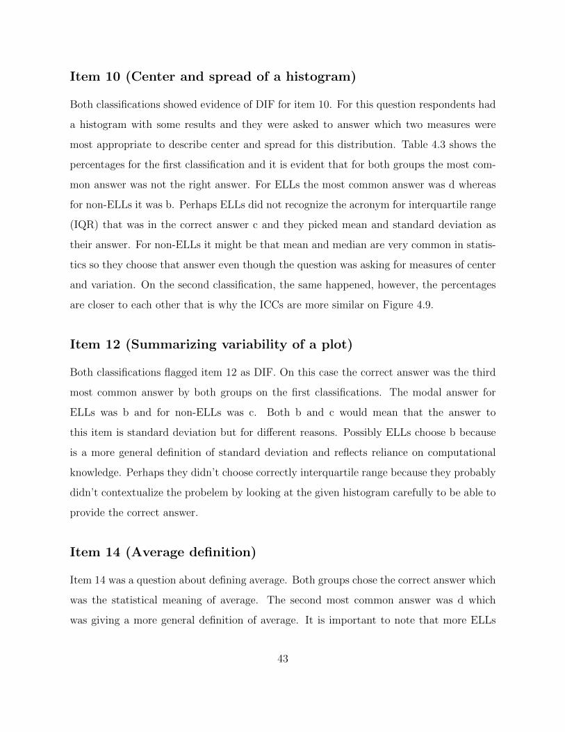
4.3.2 Item 10 (Center and spread of a histogram) . . . . . . . . . . . . . 29
4.3.3 Item 12 (Summarizing variability of a plot) . . . . . . . . . . . . . . 30
4.3.4 Item 14 (Average definition) . . . . . . . . . . . . . . . . . . . . . . 31
4.4 Individual Item Analysis Second Classification
(English proficiency) . . . . . . . . . . . . . . . . . . . . . . . . . . . . . . 32
4.4.1 Item 6 (Average family size) . . . . . . . . . . . . . . . . . . . . . . 32
4.4.2 Item 7 (Income average) . . . . . . . . . . . . . . . . . . . . . . . . 33
4.4.3 Item 8 (Finding median after adding 5 to the top scores) . . . . . . 34
4.4.4 Item 10 (Center and spread of a histogram) . . . . . . . . . . . . . 35
4.4.5 Item 12 (Summarizing variability of a plot) . . . . . . . . . . . . . . 36
4.4.6 Item 14 (Average definition) . . . . . . . . . . . . . . . . . . . . . . 37
4.4.7 Item 15 (Spread definition) . . . . . . . . . . . . . . . . . . . . . . . 38
4.5 Analysis of the last 3 items . . . . . . . . . . . . . . . . . . . . . . . . . . . 40
5 Discussion . . . . . . . . . . . . . . . . . . . . . . . . . . . . . . . . . . . . . . . 41
5.1 Individual Item Discussion . . . . . . . . . . . . . . . . . . . . . . . . . . . 41
5.2 Limitations . . . . . . . . . . . . . . . . . . . . . . . . . . . . . . . . . . . 44
x
5.3 Conclusions and Recommendations for Teaching . . . . . . . . . . . . . . . 45
References . . . . . . . . . . . . . . . . . . . . . . . . . . . . . . . . . . . . . . . . . 47
Appendix
A Survey . . . . . . . . . . . . . . . . . . . . . . . . . . . . . . . . . . . . . . . . . 50
B R-Code . . . . . . . . . . . . . . . . . . . . . . . . . . . . . . . . . . . . . . . . 59
Curriculum Vitae . . . . . . . . . . . . . . . . . . . . . . . . . . . . . . . . . . . . . 65
xi
List of Tables
3.1 Optional caption for list of figures . . . . . . . . . . . . . . . . . . . . . . . 12
3.2 Interpretation of ICC Properties for Knowledge measures . . . . . . . . . . 15
4.1 Classification of students’ year in school . . . . . . . . . . . . . . . . . . . 24
4.2 Students that were rated as ELLs and non-ELLs according to their answer
on Question 3 and 5. . . . . . . . . . . . . . . . . . . . . . . . . . . . . . . 25
4.3 *Note: Boldfaced type signifies the correct answer. Students’ answers in
percentages (%) by answer choice by native language. . . . . . . . . . . . 26
4.4 *Note: Boldfaced type signifies the correct answer. Students’ answers in
percentages (%) by answer choice by their English proficiency. . . . . . . . 26
4.5 Overall uniform and non-uniform DIF analysis for first ELL classification
(native language) . . . . . . . . . . . . . . . . . . . . . . . . . . . . . . . . 27
4.6 Overall uniform and non-uniform DIF analysis for second ELL classification
(English proficiency) . . . . . . . . . . . . . . . . . . . . . . . . . . . . . . 28
4.7 *Note: (1) refers to native language and (2) refers to English proficiency
classifications. Results. . . . . . . . . . . . . . . . . . . . . . . . . . . . . 39
5.1 Recommendations for teaching . . . . . . . . . . . . . . . . . . . . . . . . . 46
xii
List of Figures
2.1 Interaction between English and Spanish academic and everyday languages 6
2.2 Answer in Spanish shows that the student knew the concept . . . . . . . . 8
3.1 Source: Zumbo, 1999 p. 17-21 . . . . . . . . . . . . . . . . . . . . . . . . . 17
3.2 Methods for Detection DIF . . . . . . . . . . . . . . . . . . . . . . . . . . . 22
4.1 Histogram of Students’ Ages . . . . . . . . . . . . . . . . . . . . . . . . . . 24
4.2 Non-uniform DIF: ICC for focal and reference groups on Question 7 . . . . 29
4.3 Uniform DIF: ICC for focal and reference groups on Question 10 . . . . . . 30
4.4 Uniform DIF: ICC for focal and reference groups on Question 12 . . . . . . 31
4.5 Uniform DIF: ICC for focal and reference groups on Question 14 . . . . . . 32
4.6 Uniform DIF: ICC for focal and reference groups on Question 6 . . . . . . 33
4.7 Uniform DIF: ICC for focal and reference groups on Question 7 . . . . . . 34
4.8 ICC for focal and reference groups on Question 8 . . . . . . . . . . . . . . 35
4.9 ICC for focal and reference groups on Question 10 . . . . . . . . . . . . . . 36
4.10 ICC for focal and reference groups on Question 12 . . . . . . . . . . . . . . 37
4.11 ICC for focal and reference groups on Question 14 . . . . . . . . . . . . . . 38
4.12 ICC for focal and reference groups on Question 15 . . . . . . . . . . . . . . 39
xiii
Chapter 1
Introduction
1.1 Importance of Assessment of Conceptual Knowl-
edge
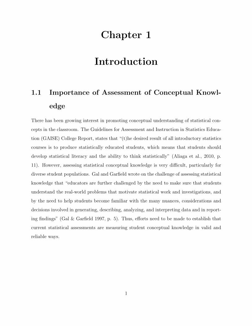
There has been growing interest in promoting conceptual understanding of statistical con-
cepts in the classroom. The Guidelines for Assessment and Instruction in Statistics Educa-
tion (GAISE) College Report, states that “(t)he desired result of all introductory statistics
courses is to produce statistically educated students, which means that students should
develop statistical literacy and the ability to think statistically” (Aliaga et al., 2010, p.
11). However, assessing statistical conceptual knowledge is very difficult, particularly for
diverse student populations. Gal and Garfield wrote on the challenge of assessing statistical
knowledge that “educators are further challenged by the need to make sure that students
understand the real-world problems that motivate statistical work and investigations, and
by the need to help students become familiar with the many nuances, considerations and
decisions involved in generating, describing, analyzing, and interpreting data and in report-
ing findings” (Gal & Garfield 1997, p. 5). Thus, efforts need to be made to establish that
current statistical assessments are measuring student conceptual knowledge in valid and
reliable ways.
1
1.2 Tests or Scales
A test is an instrument used to measure conceptual knowledge. De Ayala (2009) defines
measurement as “the process by which an attempt is made to understand the nature of a
variable (cf. Bridgman 1928)” (p. 1). For the purpose of this study, we are considering
variables that cannot be observed directly. These are latent variables or constructs. For
example, if we want to measure statistical conceptual knowledge, we cannot directly observe
the depth of knowledge. Rather, test items serve as an imperfect measure of knowledge.
There are some important points that need to be addressed before utilizing a test
measuring conceptual knowledge. First, we have to look at the reliability of the test.
Internal consistency, a component of scale reliability is used to assess the consistency of
results across items within a test. If it is consistent across time, then it is said to have high
reliability, otherwise it has low reliability. Second, we look at the validity of the test, or
whether the test actually measures what it is supposed to measure. We want to accurately
explain the latent variable by the measure. A test with good measurement properties
will have high reliability as well as high validity. The third issue is the invariance of the
test. Invariance is the property of independence between the measuring instrument and
the subjects. Finally, we need a baseline for measuring the responses, for example, on a
test we have nominal data because answers are right/wrong.
1.2.1 Example
Let us now consider an example in depth. Throughout this research we are going to be
working with the Assessment Resource Tools for Improving Statistical Thinking (ARTIST)
project (https://app.gen.umn.edu/artist/tests/index.html). This project was funded by
the NSF to create an assessment instrument that would cover the wide array of students
taking an introductory statistics course. Garfield and Gal wrote: “there is an increasing
need to develop reliable, valid, practical, and accessible assessment items and instruments”
(Garfield and Gal, 1999, p. 4). From the ARTIST project, an overall Comprehensive As-
2
sessment of Outcomes in Statistics (CAOS) was created (delMas et al, 2006). The purpose
was to find different items measuring concepts that students are expected to understand
at the end of an introductory statistics course.
1.2.2 Validation
The CAOS project was a three year research project conducted by an experienced team
of experts in education, statistics education and measurement. The ARTIST project had
an advisory board created to help with the necessary content validity for the CAOS test
as well as selection of test items. According to the advisory group feedback they created
four versions of the CAOS test: CAOS, CAOS 2, CAOS 3, and CAOS 4. Each one is
an improved version of the previous one. “An online prototype of CAOS was developed
during summer 2004, and the advisors engaged in another round of validation and feedback
in early August, 2004. The feedback was then used to produce the first version of CAOS,
which consisted of 34 multiple-choice items” (delMas et al, 2006, p. 6). On the second
round of evaluation the second version CAOS 2 was given as a pretest and post-test to
students. After the results they made changes and created the CAOS 3.
According to delMas (2006) “the third version of CAOS was given to a group of 30
statistics instructors who were faculty graders of the Advanced Placement Statistics exam
in June, 2005, for another round of validity ratings” (p. 7). With this feedback they cre-
ated the CAOS 4 version with 40 multiple choice questions. There was a final analysis
with a group of 18 members of the advisory and editorial boards of the Consortium for
the Advancement of Undergraduate Statistics Education (CAUSE). They are well known
statistics teachers at the college level as well as renowned experts in the statistics educa-
tion community. The CAOS 4 version was given to this group of experts who unanimously
agreed that the CAOS 4 measures important basic learning outcomes, and 94% agreement
that it measures important learning outcomes (delMas et al, 2006). The validation pop-
ulation included females (57.3%) and males (40.5%). The ethnicity was White (74.3%),
Black (5.1%), Asian (8.5%), and Chicano (3.6%) (Percentages do not add to 100% due to
3
missing data) (delMas et al, 2006).
1.2.3 Reliability Analysis
Out of 1028 students that took the CAOS test as a pretest and post-test 817 met the
criteria used to select students for the reliability analysis of internal consistency. Students
were required to answer all 40 questions on the test either in class using a paper test or
take an online version lasting no more than 60 minutes. The internal consistency estimate
was α = .77 (Cronbach’s alpha). This implies that the CAOS test items have satisfactory
internal consistency for the population of students taking an introductory statistics course
(delMas, 2006).
1.3 Research Question
When tests are given to new populations, some issues arise regarding validity and reliability.
When the scale is created for a certain population it might function differently when given
to another population. People with a distinct age, education level, race, or language back-
ground might be in disadvantage when the scale was only tested for one kind of population.
Our research question is to examine whether items from the ARTIST database on meth-
ods of center and variation function differently when administered to English Language
Learners (ELLs).
4
Chapter 2
ELLs in the Mathematical Sciences
The population of English Language Learners (ELL) in the United States has been growing
rapidly in the past few years. According to Goldenberg (2008), the population of ELLs in
K-12 public schools grew from 1 out of 20 in 1990 to 1 out of 9 only fifteen years later.
With this fast growth, he argues that 1 out of 4 K-12 students in the United States will
be an English Language learner in 20 years. Even though not all of this population would
attend college, there is a still a high population of ELLs in college. Just in Texas, which
has the second highest population of ELLs (832 000 ELL students compared to California
with 1.1 million ELL students): 46% of Asian ELLs, 26% of Black ELLs and 15% of
Hispanic ELLs enroll in a 4-year public college (Flores, Batalova, and Fix, 2012, p. 17).
Academic language is widely used in college courses. If an ELL is more familiar with the
everyday usage of English its very likely that he/she would struggle understanding the
higher academic language used in college.
According to Cummins (1992), there are two proficiencies acquired when someone learns
a new language: Basic Interpersonal Communicative Skills (BICS) and Cognitive Academic
Language Proficiency (CALP). BICS are required for everyday communication such as
reading, writing and listening, whereas CALP skills are necessary for an academic context.
The later the person tries to learn a new language the harder would be to acquire the
necessary CALP skills to succeed in school since the academic registers are already built in
their own language. Lesser and Winsor (2009) state that “the challenge ELLs face is that
the academic meaning of a term may be the same as the everyday meaning, different from
everyday meaning, or not have an everyday counterpart at all” (p. 8). For the purpose of
this research we would make the argument for a need of assessment for ELL students in
5
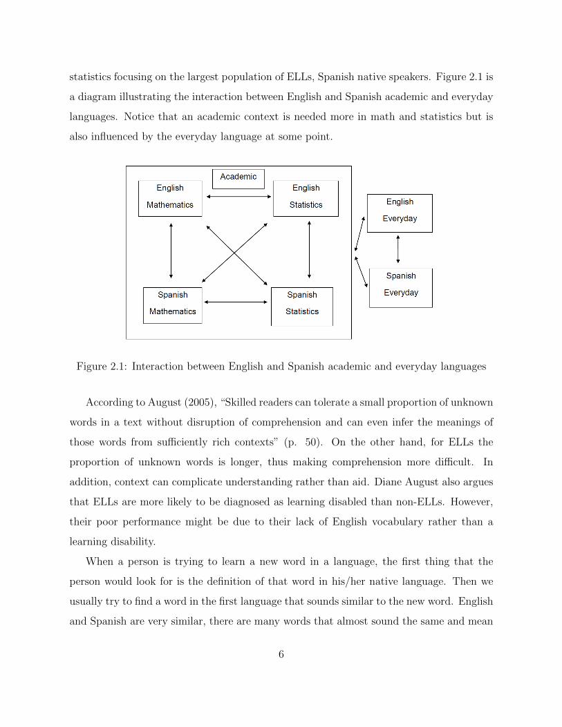
statistics focusing on the largest population of ELLs, Spanish native speakers. Figure 2.1 is
a diagram illustrating the interaction between English and Spanish academic and everyday
languages. Notice that an academic context is needed more in math and statistics but is
also influenced by the everyday language at some point.
Figure 2.1: Interaction between English and Spanish academic and everyday languages
According to August (2005), “Skilled readers can tolerate a small proportion of unknown
words in a text without disruption of comprehension and can even infer the meanings of
those words from sufficiently rich contexts” (p. 50). On the other hand, for ELLs the
proportion of unknown words is longer, thus making comprehension more difficult. In
addition, context can complicate understanding rather than aid. Diane August also argues
that ELLs are more likely to be diagnosed as learning disabled than non-ELLs. However,
their poor performance might be due to their lack of English vocabulary rather than a
learning disability.
When a person is trying to learn a new word in a language, the first thing that the
person would look for is the definition of that word in his/her native language. Then we
usually try to find a word in the first language that sounds similar to the new word. English
and Spanish are very similar, there are many words that almost sound the same and mean
6
the same thing in English and Spanish. These words are called cognates. Words such
as different/diferente or division/division might be easy to identify to a Spanish speaker
learning English. However, there are false cognates as well that might be confusing for
some such as embarrassed/embarazada sound the same but they have completely different
meanings.
Many mathematics and statistics teachers may think that their job is to teach math-
ematics not language. However, mathematics is a new language that students need to
master, a task possibly difficult for non-ELLs. Students usually need some time to adapt
to mathematics language. Yet, at the end of a course students are expected to read, under-
stand, and discuss mathematical ideas (Thompson, 2000). Thompson says that “teachers
forget that the words and phrases that are familiar to us are foreign to our students” (p.
568).
In fact, there are many reasons why a non-ELL or ELL might get confused when learning
mathematics vocabulary. One of the problems identified by Thompson (2000) is that “some
words are shared by mathematics and everyday English, but they have distinct meanings”,
for example in algebra: radical, origin, function or in statistics: mode, event, combination
(p. 569). Therefore, if an ELL has just the BICS skills he/she would struggle to find
the distinction between the mathematical meaning and the everyday meaning. Garrison
(1999) states that when dealing with a linguistically diverse classroom, teachers must first
consider the language needed as well as the language proficiency of the students in order
to provide instruction.
Another issue pointed out by Thompson (2000) was, “a single English word may trans-
late into Spanish or another language in two different ways” such as round (redondear), as
in round off, or round (redondo), as in circular (p. 569). Hence, we have another reason
to make the argument that understanding English is an important factor for ELLs in a
mathematics classroom. Garrison (1999) states the importance of adding language in the
mathematics classroom:
“As English-language learners make the transition from primary language into
7
English instruction, the English equivalents for the mathematical terms they
learned in their primary language might not be covered in the upcoming lessons,
creating gaps in their English vocabulary that are irregular and unpredictable.
Therefore, mathematics teachers should review or preview all essential vocab-
ulary at the beginning of a lesson or unit, especially when English-language
learners are in the class. New mathematical vocabulary in the second language,
however, is most effectively introduced after students have established the con-
cepts the vocabulary words represent so that they learn the new ‘label’ for the
known concept” (p. 49).
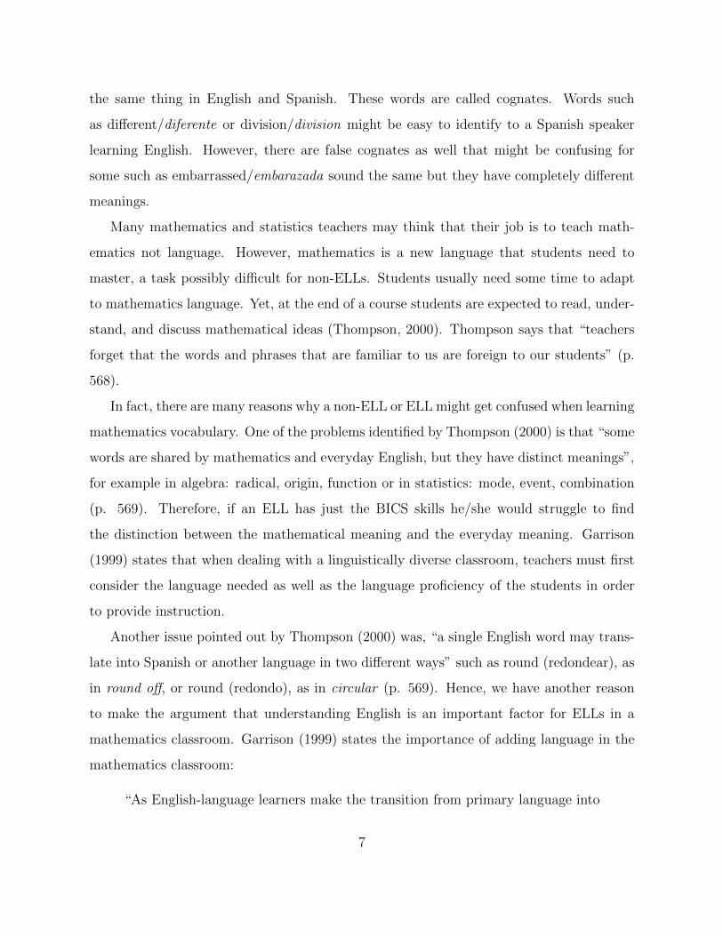
Previously, we have mentioned that poor achievement by ELLs might be confused with
a learning disability. The following example, illustrating this point, is adapted from Garri-
son’s article (Garrison & Mora, 2008 pp. 43-44). The example is work done by a student
that was a recent immigrant. When she was asked to explain the area of a triangle, her
answer in English was very limited as we can see in Figure a. However, when she was
asked to answer in Spanish her answer was considerably better (Figure b). This example
illustrates that ELLs often have the right idea; they just don’t know how to express that
idea in English.
(a) Response in English (b) Response in Spanish
Figure 2.2: Answer in Spanish shows that the student knew the concept
8
There is some research done on the language factor importance on assessing students in
mathematics. Abedi & Lord (2001) found that ELLs were at disadvantaged when solving
word problems and that modifiying the linguistic structure of the problem resulted on a
better performance for ELLs. There is another study that investigated math achievement
differences between ELLs and non-ELLs students on a literacy-based performance assess-
ment (LBPA) (Brown, 2005). Young et al (2011) also found some differences between ELLs,
former ELLs and non-ELLs on a content based assessment in math. Mahoney (2008) states
the need for large sample of students at different levels of English proficiency to create a
good assessment for ELLs in mathematics. On the statistics area, there are some discussions
about assessing students in statistics courses (Onwuegbuzie & Leech, 2003). There is also
the CAOS assessment test mentioned above (Delmas et al, 2006). Yet, these assessments
on statistics do not focus on ELLs.
There is a large body of research about assessment of ELLs in mathematics as mentioned
in the previous paragraphs. However, there is none that focuses on statistics. Nevertheless,
statistics is an important branch of mathematics and it requires an expanded vocabulary.
In statistics we are not only dealing with numerical answers but also with written responses.
Jennifer Kaplan et al (2009, 2011, 2012) have studied issues with vocabulary in statistics.
However, it is important to point out that this and related studies did not include English
Language Learners.
As we have seen, language is an important factor in mathematics and statistics achieve-
ment. There is a need to see statistics as a different subject on its own, especially for ELLs.
According to Lesser and Winsor, the distinctiveness of statistics is relevant because one or
more of the ways in which statistics is different from mathematics could plausibly affect
how ELL issues play out in a concrete way (2009). We can summarize Lesser’s findings as
follows (Lesser & Winsor, 2009 pp. 18-20):
• Students move among registers: confusion between the everyday usages of the word
with academic usages of the word (in statistics or even mathematics).
9
• Context plays an important role when explaining statistics: the way the teacher is
presenting the material is not familiar for the Spanish speaking audience.
• There may be an overlap between the previous two: confusion between mathematics
and statistics registers.
For the purpose of this research we would make the argument for a need of assessment
for ELL students in statistics focusing on the largest population of ELLs; that is native
Spanish speakers. We build upon Lesser and Winsor’s research with Spanish speakers in
an introductory statistics class concentrating on measures of center and variation.
Appendix A contains the survey items selected for this study. These items focus on mea-
sures of center and variability. This is an appropriate focus since all students encounter
these concepts in all courses early in the semester. In addition, these items utilize vocabu-
lary that may be difficult for ELLs. The Communication, Language and Statistics Survey
(CLASS) identified that ELLs experience some difficulty differentiating between the words
mean, median, and mode (Lesser, Wagler, Esquinca, & Valenzuela).
10
Chapter 3
IRT and DIF
3.1 Item Response Theory
Item Response models show the association between the correct response of an item and
the ability to answer it measured by an instrument. The instrument in most cases is
a survey or a test and the items are the questions in the instrument. IRT models can
be either dichotomous (two categories) such as correct/incorrect questions or polytomous
(more than two categories) such as poor, fair, good, excellent.
In order to predict a set of ability parameters for each person Θ, there are a set of
parameters from an IRT model called difficulty, discrimination, and guessing. First, we
consider the parameter item difficulty which is the location parameter. The location pa-
rameter, under certain conditions is the likelihood of correct response β in reference to the
ability at which 50% of the examinees will answer correctly. In more general conditions
it is the inflection point. Next, the discrimination parameter α is the difference between
examinees and their latent trait. Large discrimination parameters can easily differentiate
between examinees with high and low ability. Finally a lower asymptote or guessing pa-
rameter χ is also included in the IRT model. This parameter computes the probability that
a person with the lowest ability answers the item correctly. The IRT model can include a
lower or left asymptote and an upper or right asymptote. These are the parameters that
an IRT model may include even though these may not always be freely estimated.
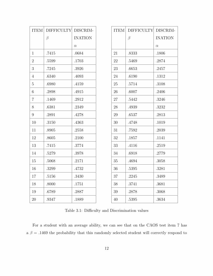
IRT models are often utilized for education scales that assess student knowledge, for
example, the CAOS test. Validation studies for educational scales estimate the difficulty
and discrimination parameters for each item as we can see in Table 3.1.
11
ITEM DIFFICULTY DISCRIM-
β INATION
α
1 .7415 .0684
2 .5599 .1703
3 .7245 .3926
4 .6340 .4093
5 .6980 .4159
6 .2898 .4915
7 .1469 .2912
8 .6381 .2349
9 .2891 .4278
10 .3150 .4363
11 .8905 .2558
12 .8605 .2100
13 .7415 .3774
14 .5279 .3978
15 .5068 .2171
16 .3299 .4732
17 .5156 .3430
18 .8000 .1751
19 .6789 .2887
20 .9347 .1889
ITEM DIFFICULTY DISCRIM-
β INATION
α
21 .8333 .1806
22 .5469 .2874
23 .6653 .2457
24 .6190 .1312
25 .5714 .3108
26 .6007 .2406
27 .5442 .3246
28 .4939 .3232
29 .6537 .2813
30 .4748 .1019
31 .7592 .2039
32 .1857 .1141
33 .4116 .2519
34 .6918 .2779
35 .4694 .3058
36 .5395 .3281
37 .2245 .3489
38 .3741 .3681
39 .2878 .3068
40 .5395 .3634
Table 3.1: Difficulty and Discrimination values
For a student with an average ability, we can see that on the CAOS test item 7 has
a β = .1469 the probability that this randomly selected student will correctly respond to
12
this item is only .1469, whereas on item 11 the probability of answering the item correctly
will be .8905. In addition, item 1 has a low discrimination value with α = .0684 thus item
1 does not differentiate well among respondents. On the other hand, item 6 has a higher
discrimination value with α = .4915, so this item differentiates well among respondents.
3.2 Dichotomous models
Dichotomous models yield the probability of a score of 1 for a correct response or 0 for
incorrect responses. The difference relies on the parameters that are being studied. In this
section, different models and their respective parameters are discussed.
3.2.1 Rasch Model:
The dichotomous Rasch Model (RM) assumes that there is a real-valued latent trait Θj for
each examinee j and a real-valued difficulty parameter βi, for each item i,
P (Yij = 1) =e(Θj−βi)
1 + e(Θj−βi)(3.1)
for all examinees j = 1, ..., N and all items i = 1, ..., I, and where N= number of students
and I= number of items.
With this definition of RM, we have that the probability of responding correctly in-
creases strictly with an increase in the parameter Θi.
3.2.2 One Parameter Logistic Model (1PL):
For the 1PL, the discrimination parameter α is the same among all examinees. The only
parameter changing for each item is the difficulty parameter β and Θ, the latent trait varies
for each examinee. The 1PL model is:
P (Yij = 1) =eα(Θj−βi)
1 + eα(Θj−βi)(3.2)
13
for all examinees j = 1, ..., N and all items i = 1, ..., I, where N = number of students and
I = number of items. The difference between the 1PL and the RM model is that the RM
model holds α = 1 whereas in the 1PL model α is freely estimated.
3.2.3 Two Parameter Logistic Model (2PL):
By allowing the discrimination parameter and difficulty parameter to vary the 2PL model
is formulated. The 2PL model is given by,
P (Yij = 1) =eαi(Θj−βi)
1 + eαi(Θj−βi)(3.3)
for all examinees j = 1, ..., N and all items i = 1, ..., I and where N = number of students
and I = number of items.
On this model Θj is the latent trait, αi is the location (discrimination) parameter
and βi is the difficulty parameter. With the 2PL model, an item provides the maximum
probability of a correct response at βi. In contrast to the 1PL, in the two parameter model
the maximum amount of information or reliability can vary from item to item as αi varies
across items (DeAyala 2009, p. 119).
3.2.4 Three Parameter Logistic Model (3PL):
The 3PL model adds a lower asymptote parameter, called the guessing parameter. To
better explain this parameter, we can look at an examinee that is taking a test in a com-
pletely different language than the one he/she speaks. The examinee does not understand
this language so there is a probability of answering correct just by guessing. In this case
the guessing parameter would be χi and most of the time this parameter is higher than
chance. We also add the difficulty and discrimination parameters as in in the 2PL model.
The equation is:
P (Yij = 1) = χi + (1− χi)eαi(Θj−βi)
1 + eαi(Θj−βi)(3.4)
for all examinees j = 1, ..., N and all items i = 1, ..., I, and where N= number of students
and I= number of items.
14
3.3 Item Characteristic Curve
The item characteristic curve (ICC) is the relationship between examinees’ item perfor-
mance and the underlying variable of interest. We use a logistic function and the X-axis is
the latent variable or ability and the Y-axis is the probability of getting the item correct.
It is very common that the X-axis goes from −3 to +3.
The following table explains the ICC properties related to the IRT models:
ICC Property Knowledge
Position along the X-axis Item difficulty
(β parameter) Amount of aptitude to get an item right
Slope Item discrimination
(α parameter) Flat ICC does not
differentiate among
test takers
Y-intercept Guessing
(χ parameter)
Table 3.2: Interpretation of ICC Properties for Knowledge measures
3.4 Estimation Method: Joint Maximum Likelihood
For the 3PL model, we will be using joint maximum likelihood to estimate the parameters.
This estimation procedure consists of finding the set of item and person parameters that
would maximize the likelihood of the observed item responses. The likelihood equation is
as follows:
L(θ, a, b, c; y) =I∏j=1
n∏i=1
Pi(θj; ai, bi, ci)yij [1− Pi(θj; ai, bi, ci)]1−yij (3.5)
Where yij is the response to item i by person j.
15
We maximized the logarithm of the likelihood mentioned above and this is the set of
estimation equations:
∂
∂θj=
I∑i=1
[cia1D + ai(1− ci)E − aiF ] = 0
∂
∂ai=
N∑j=1
[ci(θj − bi)D + (1− ci)(θj − bi)E − (θj − bi)F ] = 0
∂
∂bi=
N∑j=1
[−cia1D − ai(1− ci)E + aiF ] = 0 (3.6)
∂
∂ci=
N∑j=1
[D − ai(θj − bi)E] = 0
Where:
D =yijexp{ai(θj − bi)}1 + ciexp{(θj − bi)}
E = (1− yij) (3.7)
F =exp{ai(θj − bi)}
1 + exp{ai(θj − bi)}
We can find the solutions of these equations by starting with an initial value of the
ability parameters and solving for the item parameters, then holding the item parameters
fixed, and solving for an improved estimate of the ability parameter values, and so on. This
technique was done by Birnbaum and it’s called the joint maximum likelihood (JML) (van
der Linden & Hambleton, 1997 p. 15).
3.5 Differential Item Functioning
Differential Item Functioning (DIF) or measurement bias refers to “differences in the way a
test item functions across demographic groups that are matched on the attribute measured
by the test or the test item” (Osterlind 2009, p.8). For a more formal definition, we can
have any of the previous models where Y = 1 is the response to a particular question on a
16
test or survey. We also have the ability or latent trait denoted by Θ. So we would express
the conditional probability of Y given Θ as f(Y |Θ). On the DIF case we want to compare
the answers of the conditional probability within two groups which we would called “focal”
and “reference” groups. Even though there is no difference between which group will be
the reference or the focal, it is common to name the group for which we think the test or
survey will favor as the reference group. Thus, that group in disadvantage will be the focal
group. If there is no DIF and the measurement errors distribution are the same for both
group we have the following:
f(Y |Θ, G = R) = f(Y |Θ, G = F ) (3.8)
Where G is the grouping variable, R is the reference group, and F is the focal group.
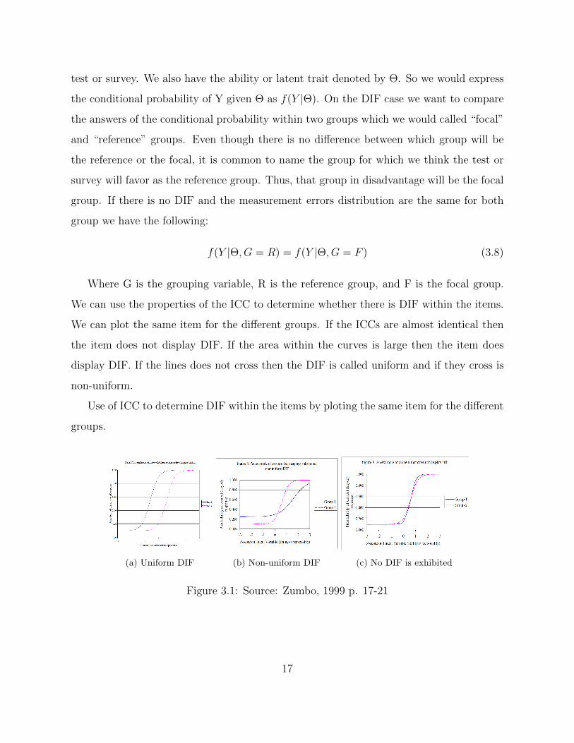
We can use the properties of the ICC to determine whether there is DIF within the items.
We can plot the same item for the different groups. If the ICCs are almost identical then
the item does not display DIF. If the area within the curves is large then the item does
display DIF. If the lines does not cross then the DIF is called uniform and if they cross is
non-uniform.
Use of ICC to determine DIF within the items by ploting the same item for the different
groups.
(a) Uniform DIF (b) Non-uniform DIF (c) No DIF is exhibited
Figure 3.1: Source: Zumbo, 1999 p. 17-21
17
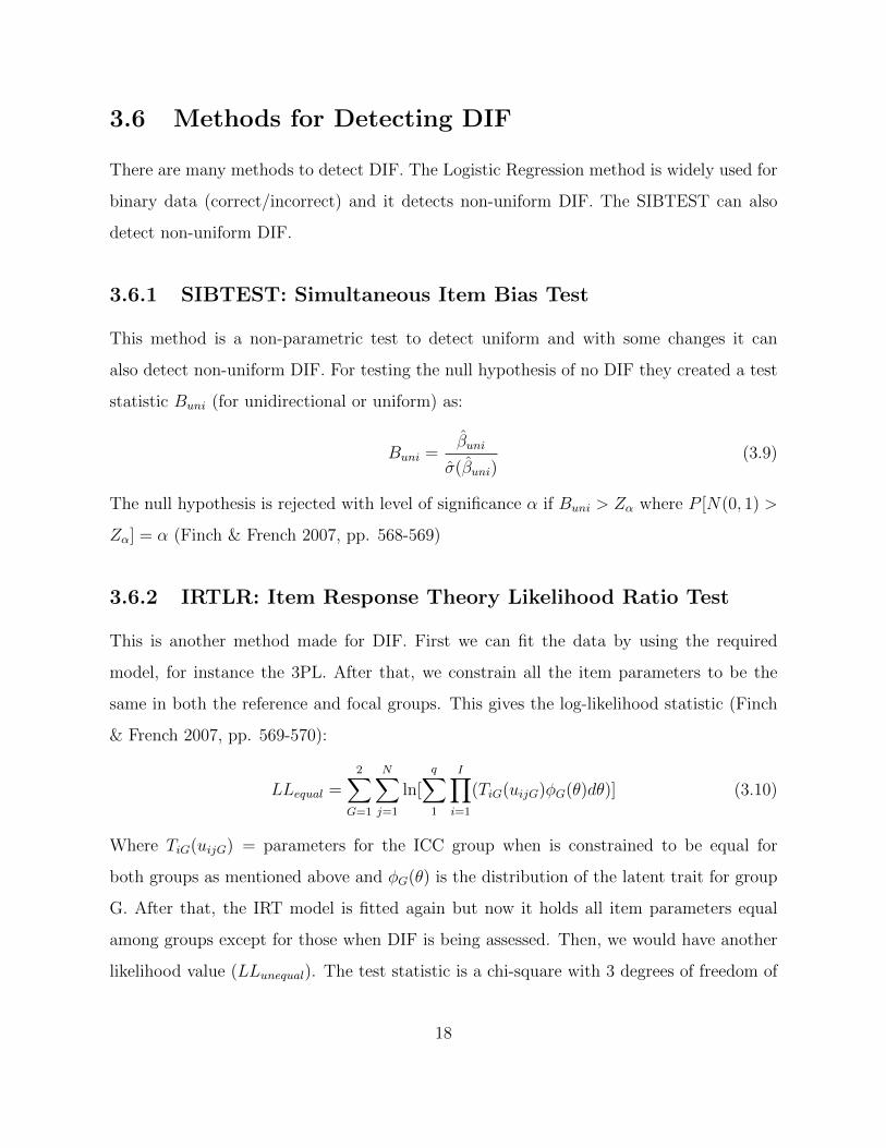
3.6 Methods for Detecting DIF
There are many methods to detect DIF. The Logistic Regression method is widely used for
binary data (correct/incorrect) and it detects non-uniform DIF. The SIBTEST can also
detect non-uniform DIF.
3.6.1 SIBTEST: Simultaneous Item Bias Test
This method is a non-parametric test to detect uniform and with some changes it can
also detect non-uniform DIF. For testing the null hypothesis of no DIF they created a test
statistic Buni (for unidirectional or uniform) as:
Buni =β̂uni
σ̂(β̂uni)(3.9)
The null hypothesis is rejected with level of significance α if Buni > Zα where P [N(0, 1) >
Zα] = α (Finch & French 2007, pp. 568-569)
3.6.2 IRTLR: Item Response Theory Likelihood Ratio Test
This is another method made for DIF. First we can fit the data by using the required
model, for instance the 3PL. After that, we constrain all the item parameters to be the
same in both the reference and focal groups. This gives the log-likelihood statistic (Finch
& French 2007, pp. 569-570):
LLequal =2∑
G=1
N∑j=1
ln[
q∑1
I∏i=1
(TiG(uijG)φG(θ)dθ)] (3.10)
Where TiG(uijG) = parameters for the ICC group when is constrained to be equal for
both groups as mentioned above and φG(θ) is the distribution of the latent trait for group
G. After that, the IRT model is fitted again but now it holds all item parameters equal
among groups except for those when DIF is being assessed. Then, we would have another
likelihood value (LLunequal). The test statistic is a chi-square with 3 degrees of freedom of
18
the difference between the two values computed before G2 = −2(LLequal − LLunequal). If
the test is significant then there is DIF, we can also test each parameter individually by a
chi-square with 1 degree of freedom.
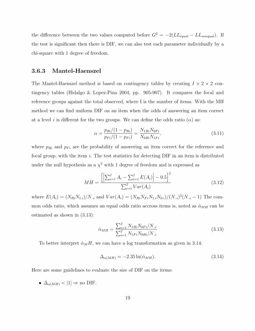
3.6.3 Mantel-Haenszel
The Mantel-Haenszel method is based on contingency tables by creating I × 2 × 2 con-
tingency tables (Hidalgo & Lopez-Pina 2004, pp. 905-907). It compares the focal and
reference groups against the total observed, where I is the number of items. With the MH
method we can find uniform DIF on an item when the odds of answering an item correct
at a level i is different for the two groups. We can define the odds ratio (α) as:
α =pRi/(1− pRi)pFi/(1− pFi)
=N1RiN0Fi
N0RiN1Fi
, (3.11)
where pRi and pFi are the probability of answering an item correct for the reference and
focal group, with the item i. The test statistics for detecting DIF in an item is distributed
under the null hypothesis as a χ2 with 1 degree of freedom and is expressed as
MH =
[∣∣∣∑Ii=1Ai −
∑Ii=1 E(Ai)
∣∣∣− 0.5]2
∑Ii=1 V ar(Ai)
(3.12)
where E(Ai) = (NRiN1.i)/N..i and V ar(Ai) = (NRiNFiN1.iN0.i)/(N..i)2(N..i − 1) The com-
mon odds ratio, which assumes an equal odds ratio accross items is, noted as α̂MH can be
estimated as shown in (3.13):
α̂MH =
∑Ii=1N1RiN0Fi/N..i∑Ii=1N1FiN0Ri/N..i
(3.13)
To better interpret α̂MH, we can have a log transformation as given in 3.14:
∆α(MH) = −2.35 ln(α̂MH). (3.14)
Here are some guidelines to evaluate the size of DIF on the items:
• ∆α(MH) < |1| ⇒ no DIF.
19
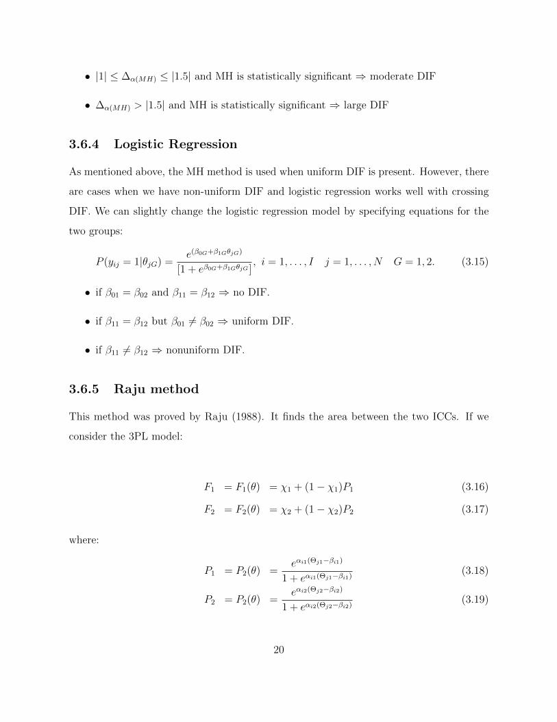
• |1| ≤ ∆α(MH) ≤ |1.5| and MH is statistically significant ⇒ moderate DIF
• ∆α(MH) > |1.5| and MH is statistically significant ⇒ large DIF
3.6.4 Logistic Regression
As mentioned above, the MH method is used when uniform DIF is present. However, there
are cases when we have non-uniform DIF and logistic regression works well with crossing
DIF. We can slightly change the logistic regression model by specifying equations for the
two groups:
P (yij = 1|θjG) =e(β0G+β1GθjG)
[1 + eβ0G+β1GθjG ], i = 1, . . . , I j = 1, . . . , N G = 1, 2. (3.15)
• if β01 = β02 and β11 = β12 ⇒ no DIF.
• if β11 = β12 but β01 6= β02 ⇒ uniform DIF.
• if β11 6= β12 ⇒ nonuniform DIF.
3.6.5 Raju method
This method was proved by Raju (1988). It finds the area between the two ICCs. If we
consider the 3PL model:
F1 = F1(θ) = χ1 + (1− χ1)P1 (3.16)
F2 = F2(θ) = χ2 + (1− χ2)P2 (3.17)
where:
P1 = P2(θ) =eαi1(Θj1−βi1)
1 + eαi1(Θj1−βi1)(3.18)
P2 = P2(θ) =eαi2(Θj2−βi2)
1 + eαi2(Θj2−βi2)(3.19)
20
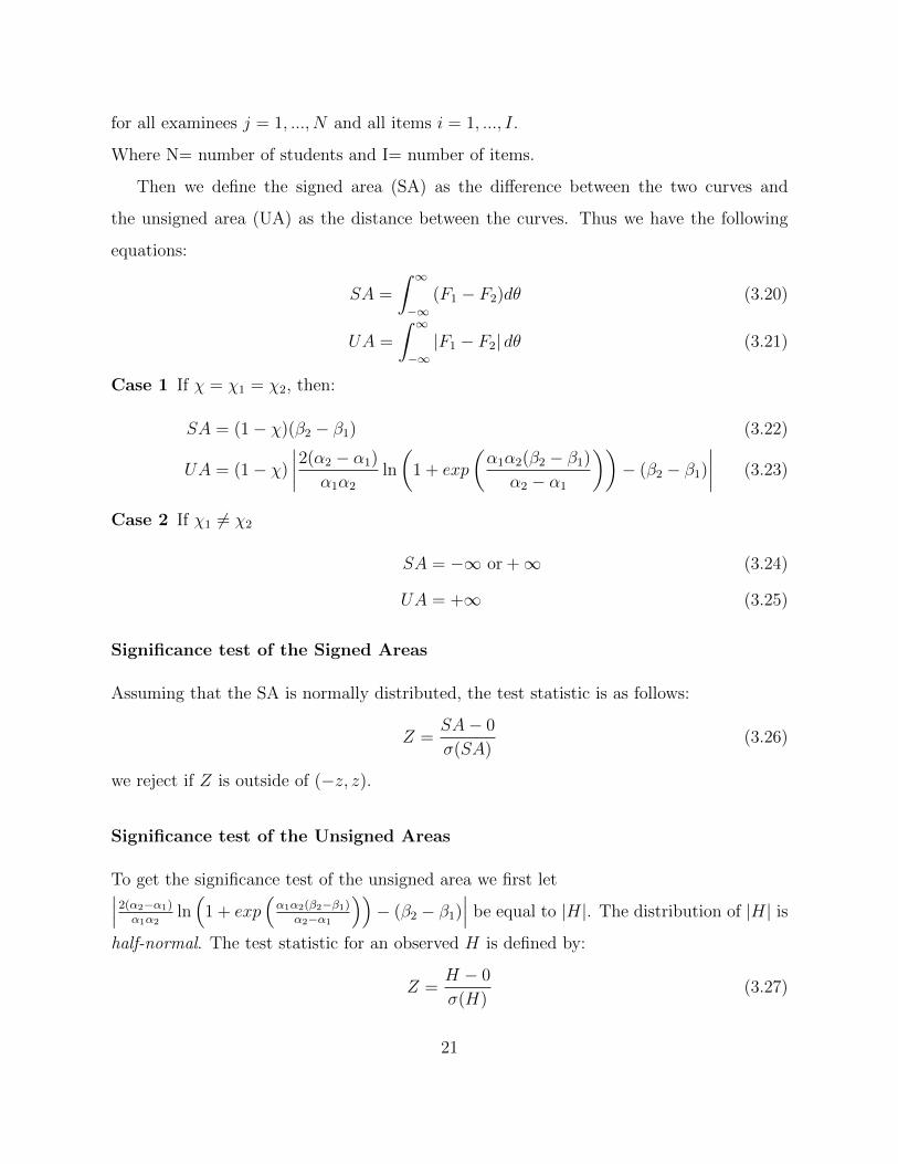
for all examinees j = 1, ..., N and all items i = 1, ..., I.
Where N= number of students and I= number of items.
Then we define the signed area (SA) as the difference between the two curves and
the unsigned area (UA) as the distance between the curves. Thus we have the following
equations:
SA =
∫ ∞−∞
(F1 − F2)dθ (3.20)
UA =
∫ ∞−∞|F1 − F2| dθ (3.21)
Case 1 If χ = χ1 = χ2, then:
SA = (1− χ)(β2 − β1) (3.22)
UA = (1− χ)
∣∣∣∣2(α2 − α1)
α1α2
ln
(1 + exp
(α1α2(β2 − β1)
α2 − α1
))− (β2 − β1)
∣∣∣∣ (3.23)
Case 2 If χ1 6= χ2
SA = −∞ or +∞ (3.24)
UA = +∞ (3.25)
Significance test of the Signed Areas
Assuming that the SA is normally distributed, the test statistic is as follows:
Z =SA− 0
σ(SA)(3.26)
we reject if Z is outside of (−z, z).
Significance test of the Unsigned Areas
To get the significance test of the unsigned area we first let∣∣∣2(α2−α1)α1α2
ln(
1 + exp(α1α2(β2−β1)
α2−α1
))− (β2 − β1)
∣∣∣ be equal to |H|. The distribution of |H| is
half-normal. The test statistic for an observed H is defined by:
Z =H − 0
σ(H)(3.27)
21
where we also reject if H lies outside the limits of (−z, z).
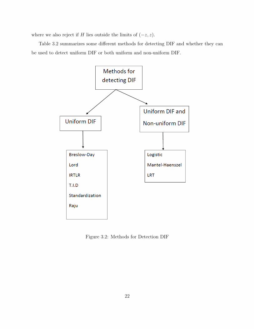
Table 3.2 summarizes some different methods for detecting DIF and whether they can
be used to detect uniform DIF or both uniform and non-uniform DIF.
Figure 3.2: Methods for Detection DIF
22
Chapter 4
Analysis
4.1 Population
The survey was given to students taking an introductory statistics class at a large urban bi-
national research university located in the Southwest and a large community college system
in a large Southwestern urban environment both located by the Mexican border. Approx-
imately 76% of the student population at this university as well as the city population is
Hispanic and a percentage of the student population are Mexican nationals. This popula-
tion is a good target for this type of research due to the extensive proportion of Spanish
speakers. The survey was administered during the Fall 2011 and Spring 2012 semesters.
There was an option to take the survey as a paper based survey or an online version. Both
versions took no more than 10 minutes to administer. The survey was not mandatory
and they had the option to withdraw. The survey was administered around 2/3 of the
Fall semester and in the middle of the Spring to assure that the teacher had covered the
material needed for the survey.
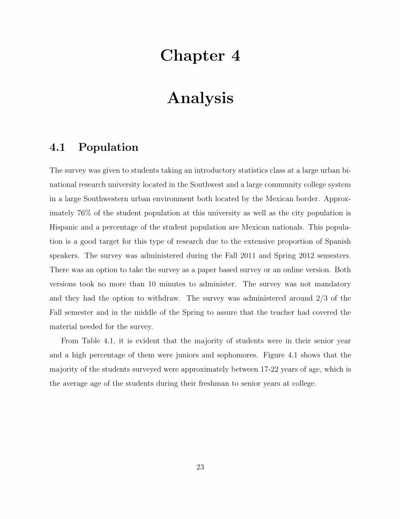
From Table 4.1, it is evident that the majority of students were in their senior year
and a high percentage of them were juniors and sophomores. Figure 4.1 shows that the
majority of the students surveyed were approximately between 17-22 years of age, which is
the average age of the students during their freshman to senior years at college.
23
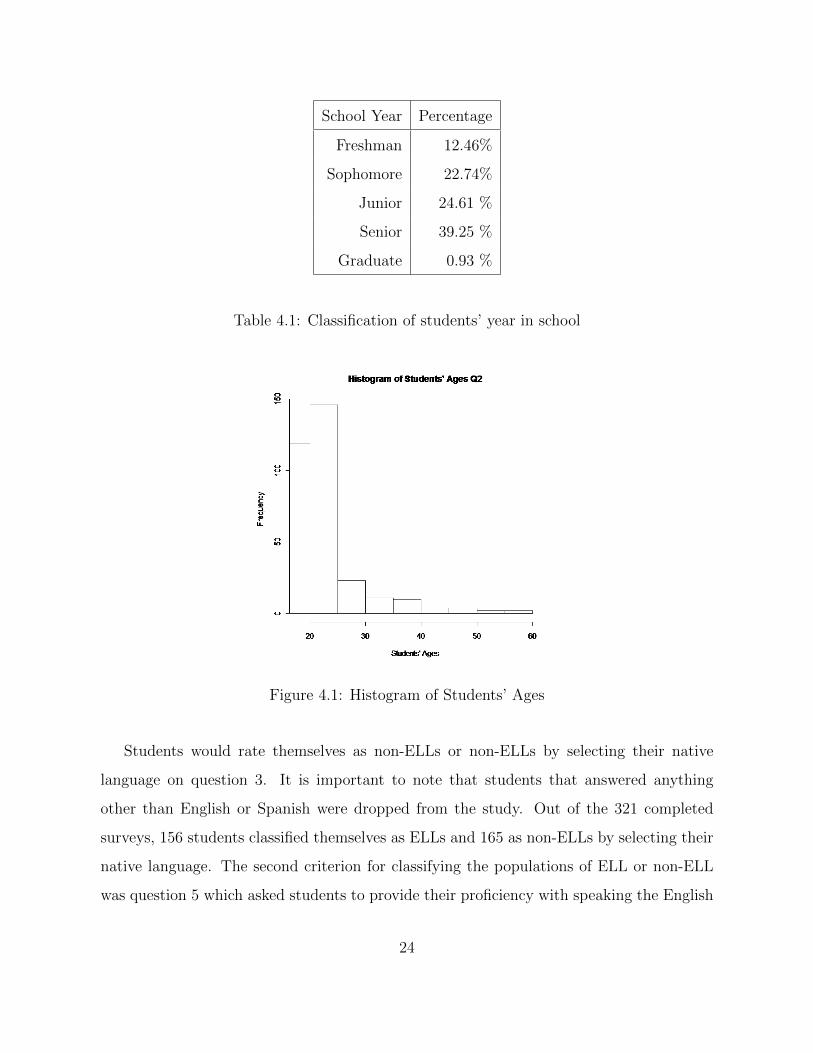
School Year Percentage
Freshman 12.46%
Sophomore 22.74%
Junior 24.61 %
Senior 39.25 %
Graduate 0.93 %
Table 4.1: Classification of students’ year in school
Figure 4.1: Histogram of Students’ Ages
Students would rate themselves as non-ELLs or non-ELLs by selecting their native
language on question 3. It is important to note that students that answered anything
other than English or Spanish were dropped from the study. Out of the 321 completed
surveys, 156 students classified themselves as ELLs and 165 as non-ELLs by selecting their
native language. The second criterion for classifying the populations of ELL or non-ELL
was question 5 which asked students to provide their proficiency with speaking the English
24
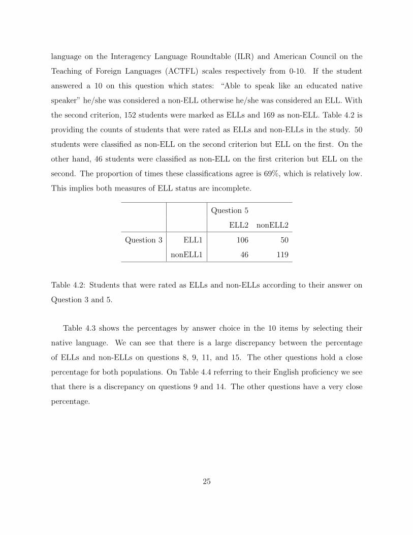
language on the Interagency Language Roundtable (ILR) and American Council on the
Teaching of Foreign Languages (ACTFL) scales respectively from 0-10. If the student
answered a 10 on this question which states: “Able to speak like an educated native
speaker” he/she was considered a non-ELL otherwise he/she was considered an ELL. With
the second criterion, 152 students were marked as ELLs and 169 as non-ELL. Table 4.2 is
providing the counts of students that were rated as ELLs and non-ELLs in the study. 50
students were classified as non-ELL on the second criterion but ELL on the first. On the
other hand, 46 students were classified as non-ELL on the first criterion but ELL on the
second. The proportion of times these classifications agree is 69%, which is relatively low.
This implies both measures of ELL status are incomplete.
Question 5
ELL2 nonELL2
Question 3 ELL1 106 50
nonELL1 46 119
Table 4.2: Students that were rated as ELLs and non-ELLs according to their answer on
Question 3 and 5.
Table 4.3 shows the percentages by answer choice in the 10 items by selecting their
native language. We can see that there is a large discrepancy between the percentage
of ELLs and non-ELLs on questions 8, 9, 11, and 15. The other questions hold a close
percentage for both populations. On Table 4.4 referring to their English proficiency we see
that there is a discrepancy on questions 9 and 14. The other questions have a very close
percentage.
25
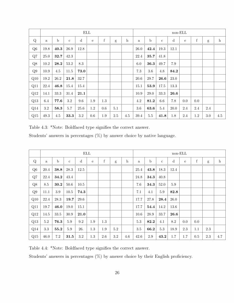
ELL non-ELL
Q a b c d e f g h a b c d e f g h
Q6 19.8 40.3 26.9 12.8 26.0 42.4 19.3 12.1
Q7 25.0 32.7 42.3 22.4 35.7 41.8
Q8 10.2 28.2 53.2 8.3 6.0 36.3 49.7 7.9
Q9 10.9 4.5 11.5 73.0 7.3 3.6 4.8 84.2
Q10 19.2 26.2 21.8 32.7 20.6 29.7 26.6 23.0
Q11 22.4 46.8 15.4 15.4 15.1 53.9 17.5 13.3
Q12 14.1 33.3 31.4 21.1 10.9 29.0 33.3 26.6
Q13 6.4 77.6 3.2 9.6 1.9 1.3 4.2 81.2 6.6 7.8 0.0 0.0
Q14 3.2 58.3 5.7 25.6 1.2 0.6 5.1 3.6 63.6 5.4 20.0 2.4 2.4 2.4
Q15 49.3 4.5 33.3 3.2 0.6 1.9 2.5 4.5 39.4 5.5 41.8 1.8 2.4 1.2 3.0 4.5
Table 4.3: *Note: Boldfaced type signifies the correct answer.
Students’ answers in percentages (%) by answer choice by native language.
ELL non-ELL
Q a b c d e f g h a b c d e f g h
Q6 20.4 38.8 28.3 12.5 25.4 43.8 18.3 12.4
Q7 22.4 34.2 43.4 24.8 34.3 40.8
Q8 8.5 30.2 50.6 10.5 7.6 34.3 52.0 5.9
Q9 11.1 3.9 10.5 74.3 7.1 4.1 5.9 82.8
Q10 22.4 28.3 19.7 29.6 17.7 27.8 28.4 26.0
Q11 19.7 46.0 19.0 15.1 17.7 54.4 14.2 13.6
Q12 14.5 33.5 30.9 21.0 10.6 28.9 33.7 26.6
Q13 5.2 76.3 5.9 9.2 1.9 1.3 5.3 82.2 4.1 8.2 0.0 0.0
Q14 3.3 55.2 5.9 26. 1.3 1.9 5.2 3.5 66.2 5.3 18.9 2.3 1.1 2.3
Q15 46.0 7.2 31.5 3.2 1.3 2.6 3.2 4.6 42.6 2.9 43.2 1.7 1.7 0.5 2.3 4.7
Table 4.4: *Note: Boldfaced type signifies the correct answer.
Students’ answers in percentages (%) by answer choice by their English proficiency.
26
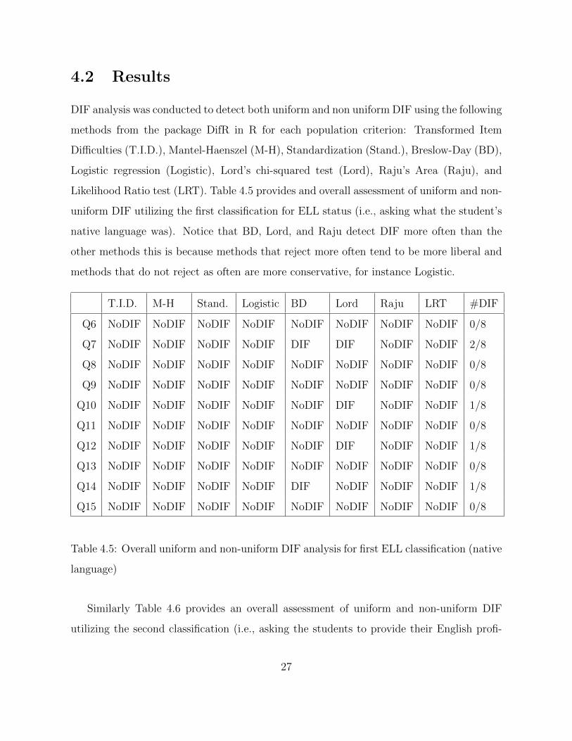
4.2 Results
DIF analysis was conducted to detect both uniform and non uniform DIF using the following
methods from the package DifR in R for each population criterion: Transformed Item
Difficulties (T.I.D.), Mantel-Haenszel (M-H), Standardization (Stand.), Breslow-Day (BD),
Logistic regression (Logistic), Lord’s chi-squared test (Lord), Raju’s Area (Raju), and
Likelihood Ratio test (LRT). Table 4.5 provides and overall assessment of uniform and non-
uniform DIF utilizing the first classification for ELL status (i.e., asking what the student’s
native language was). Notice that BD, Lord, and Raju detect DIF more often than the
other methods this is because methods that reject more often tend to be more liberal and
methods that do not reject as often are more conservative, for instance Logistic.
T.I.D. M-H Stand. Logistic BD Lord Raju LRT #DIF
Q6 NoDIF NoDIF NoDIF NoDIF NoDIF NoDIF NoDIF NoDIF 0/8
Q7 NoDIF NoDIF NoDIF NoDIF DIF DIF NoDIF NoDIF 2/8
Q8 NoDIF NoDIF NoDIF NoDIF NoDIF NoDIF NoDIF NoDIF 0/8
Q9 NoDIF NoDIF NoDIF NoDIF NoDIF NoDIF NoDIF NoDIF 0/8
Q10 NoDIF NoDIF NoDIF NoDIF NoDIF DIF NoDIF NoDIF 1/8
Q11 NoDIF NoDIF NoDIF NoDIF NoDIF NoDIF NoDIF NoDIF 0/8
Q12 NoDIF NoDIF NoDIF NoDIF NoDIF DIF NoDIF NoDIF 1/8
Q13 NoDIF NoDIF NoDIF NoDIF NoDIF NoDIF NoDIF NoDIF 0/8
Q14 NoDIF NoDIF NoDIF NoDIF DIF NoDIF NoDIF NoDIF 1/8
Q15 NoDIF NoDIF NoDIF NoDIF NoDIF NoDIF NoDIF NoDIF 0/8
Table 4.5: Overall uniform and non-uniform DIF analysis for first ELL classification (native
language)
Similarly Table 4.6 provides an overall assessment of uniform and non-uniform DIF
utilizing the second classification (i.e., asking the students to provide their English profi-
27
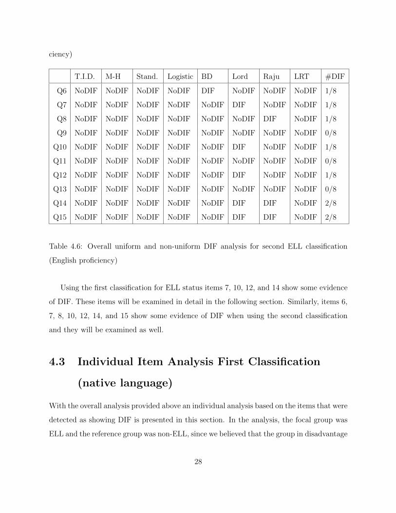
ciency)
T.I.D. M-H Stand. Logistic BD Lord Raju LRT #DIF
Q6 NoDIF NoDIF NoDIF NoDIF DIF NoDIF NoDIF NoDIF 1/8
Q7 NoDIF NoDIF NoDIF NoDIF NoDIF DIF NoDIF NoDIF 1/8
Q8 NoDIF NoDIF NoDIF NoDIF NoDIF NoDIF DIF NoDIF 1/8
Q9 NoDIF NoDIF NoDIF NoDIF NoDIF NoDIF NoDIF NoDIF 0/8
Q10 NoDIF NoDIF NoDIF NoDIF NoDIF DIF NoDIF NoDIF 1/8
Q11 NoDIF NoDIF NoDIF NoDIF NoDIF NoDIF NoDIF NoDIF 0/8
Q12 NoDIF NoDIF NoDIF NoDIF NoDIF DIF NoDIF NoDIF 1/8
Q13 NoDIF NoDIF NoDIF NoDIF NoDIF NoDIF NoDIF NoDIF 0/8
Q14 NoDIF NoDIF NoDIF NoDIF NoDIF DIF DIF NoDIF 2/8
Q15 NoDIF NoDIF NoDIF NoDIF NoDIF DIF DIF NoDIF 2/8
Table 4.6: Overall uniform and non-uniform DIF analysis for second ELL classification
(English proficiency)
Using the first classification for ELL status items 7, 10, 12, and 14 show some evidence
of DIF. These items will be examined in detail in the following section. Similarly, items 6,
7, 8, 10, 12, 14, and 15 show some evidence of DIF when using the second classification
and they will be examined as well.
4.3 Individual Item Analysis First Classification
(native language)
With the overall analysis provided above an individual analysis based on the items that were
detected as showing DIF is presented in this section. In the analysis, the focal group was
ELL and the reference group was non-ELL, since we believed that the group in disadvantage
28
is ELLs (i.e. ELLs were not expected to do as well as non-ELLs).
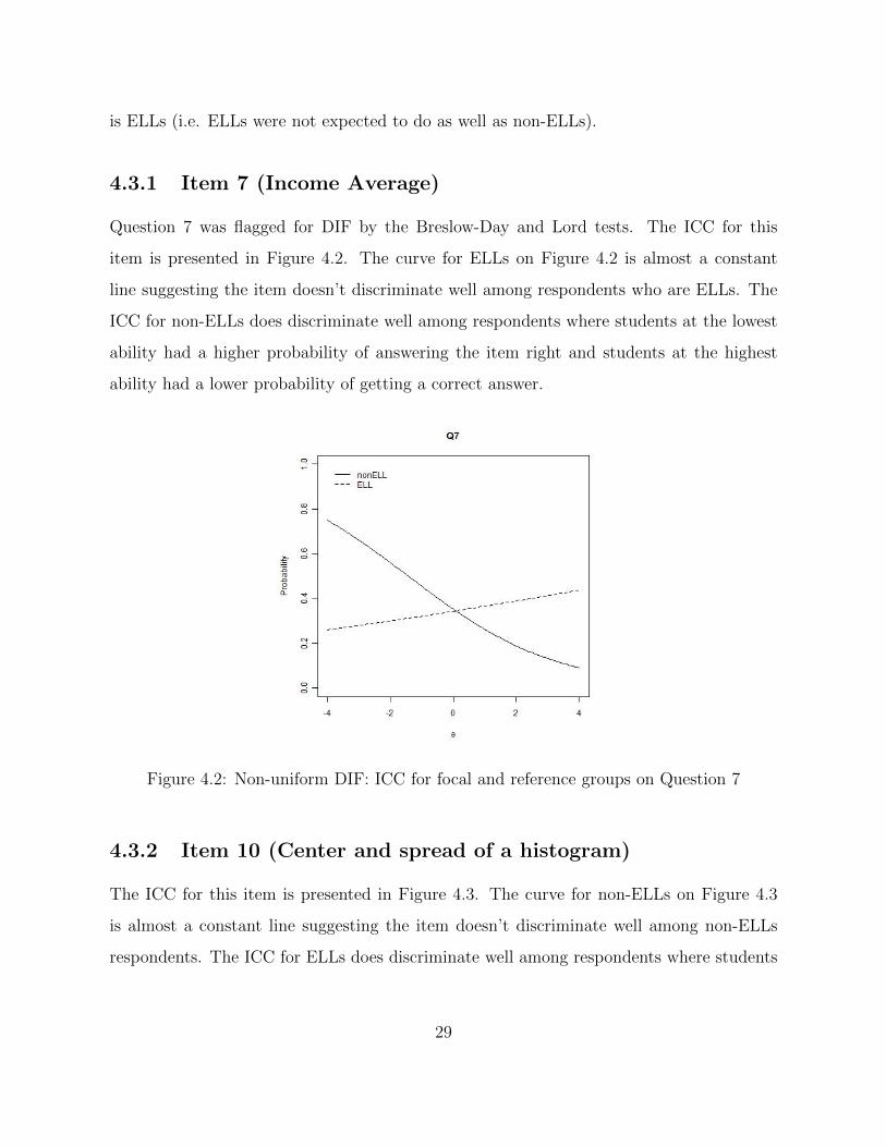
4.3.1 Item 7 (Income Average)
Question 7 was flagged for DIF by the Breslow-Day and Lord tests. The ICC for this
item is presented in Figure 4.2. The curve for ELLs on Figure 4.2 is almost a constant
line suggesting the item doesn’t discriminate well among respondents who are ELLs. The
ICC for non-ELLs does discriminate well among respondents where students at the lowest
ability had a higher probability of answering the item right and students at the highest
ability had a lower probability of getting a correct answer.
Figure 4.2: Non-uniform DIF: ICC for focal and reference groups on Question 7
4.3.2 Item 10 (Center and spread of a histogram)
The ICC for this item is presented in Figure 4.3. The curve for non-ELLs on Figure 4.3
is almost a constant line suggesting the item doesn’t discriminate well among non-ELLs
respondents. The ICC for ELLs does discriminate well among respondents where students
29
at the lowest ability had a lower probability of answering the item right and students at
the highest ability had a higher probability of getting a correct answer.
Figure 4.3: Uniform DIF: ICC for focal and reference groups on Question 10
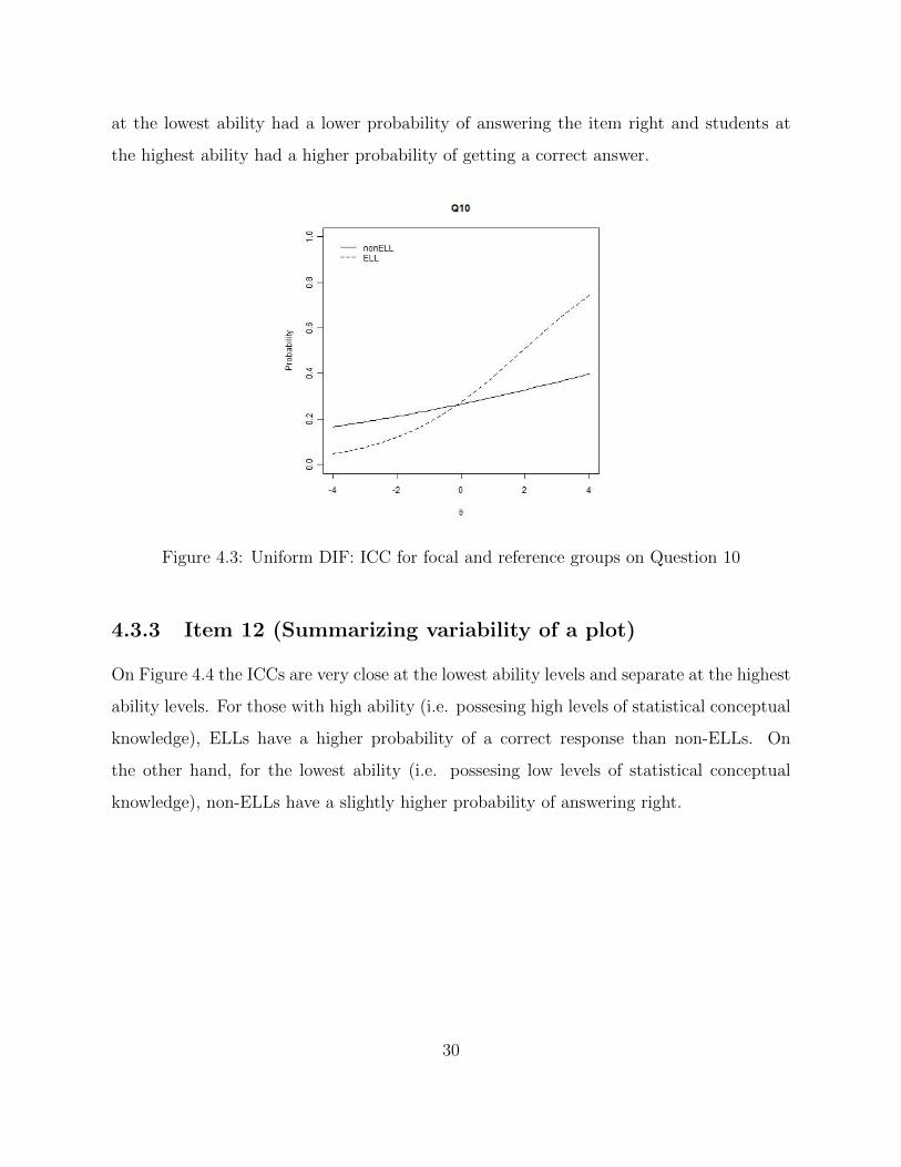
4.3.3 Item 12 (Summarizing variability of a plot)
On Figure 4.4 the ICCs are very close at the lowest ability levels and separate at the highest
ability levels. For those with high ability (i.e. possesing high levels of statistical conceptual
knowledge), ELLs have a higher probability of a correct response than non-ELLs. On
the other hand, for the lowest ability (i.e. possesing low levels of statistical conceptual
knowledge), non-ELLs have a slightly higher probability of answering right.
30
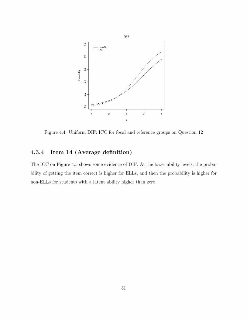
Figure 4.4: Uniform DIF: ICC for focal and reference groups on Question 12
4.3.4 Item 14 (Average definition)
The ICC on Figure 4.5 shows some evidence of DIF. At the lower ability levels, the proba-
bility of getting the item correct is higher for ELLs, and then the probability is higher for
non-ELLs for students with a latent ability higher than zero.
31
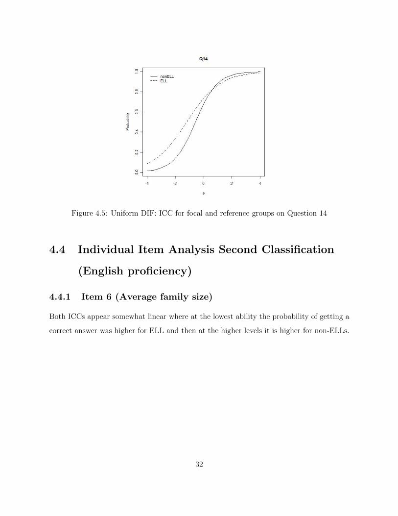
Figure 4.5: Uniform DIF: ICC for focal and reference groups on Question 14
4.4 Individual Item Analysis Second Classification
(English proficiency)
4.4.1 Item 6 (Average family size)
Both ICCs appear somewhat linear where at the lowest ability the probability of getting a
correct answer was higher for ELL and then at the higher levels it is higher for non-ELLs.
32
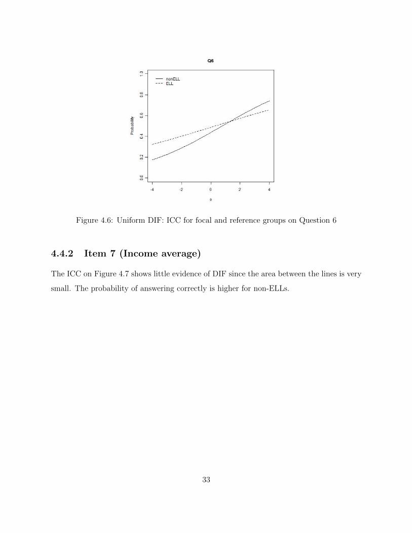
Figure 4.6: Uniform DIF: ICC for focal and reference groups on Question 6
4.4.2 Item 7 (Income average)
The ICC on Figure 4.7 shows little evidence of DIF since the area between the lines is very
small. The probability of answering correctly is higher for non-ELLs.
33

Figure 4.7: Uniform DIF: ICC for focal and reference groups on Question 7
4.4.3 Item 8 (Finding median after adding 5 to the top scores)
Figure 4.8 displays the ICC for the second classification on item 8. The ICC for ELLs
is more linear with a positive slope, whereas the ICC plot for non-ELL follows a logistic
curve. Also, at the lowest levels of ability the probability of getting a correct answer was
higher for ELLs and the opposite for the higher levels.
34
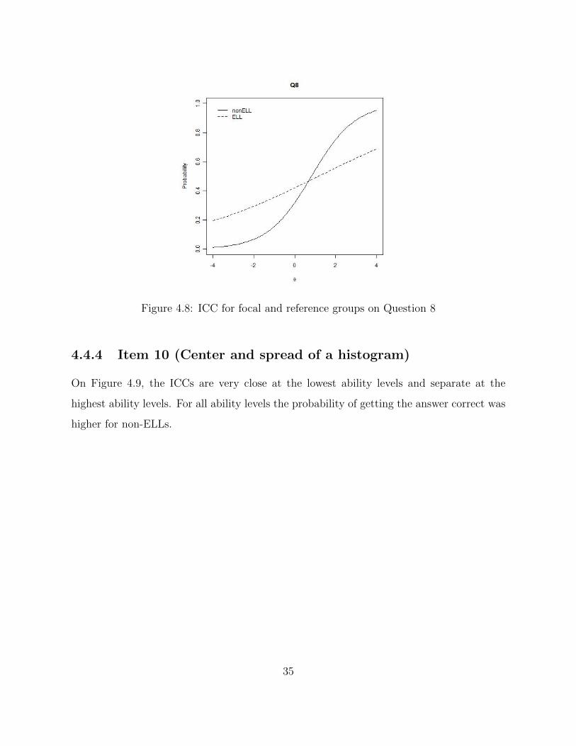
Figure 4.8: ICC for focal and reference groups on Question 8
4.4.4 Item 10 (Center and spread of a histogram)
On Figure 4.9, the ICCs are very close at the lowest ability levels and separate at the
highest ability levels. For all ability levels the probability of getting the answer correct was
higher for non-ELLs.
35
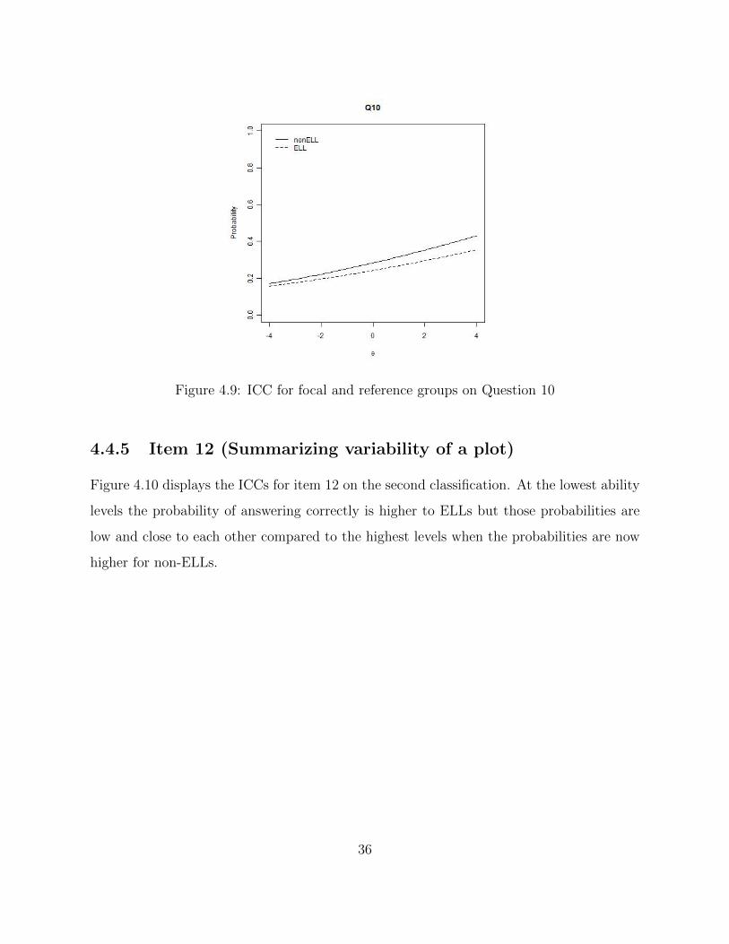
Figure 4.9: ICC for focal and reference groups on Question 10
4.4.5 Item 12 (Summarizing variability of a plot)
Figure 4.10 displays the ICCs for item 12 on the second classification. At the lowest ability
levels the probability of answering correctly is higher to ELLs but those probabilities are
low and close to each other compared to the highest levels when the probabilities are now
higher for non-ELLs.
36
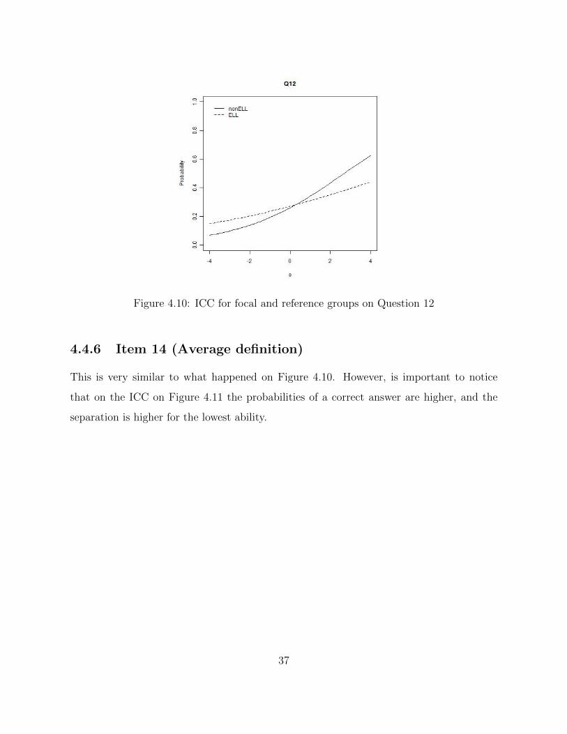
Figure 4.10: ICC for focal and reference groups on Question 12
4.4.6 Item 14 (Average definition)
This is very similar to what happened on Figure 4.10. However, is important to notice
that on the ICC on Figure 4.11 the probabilities of a correct answer are higher, and the
separation is higher for the lowest ability.
37
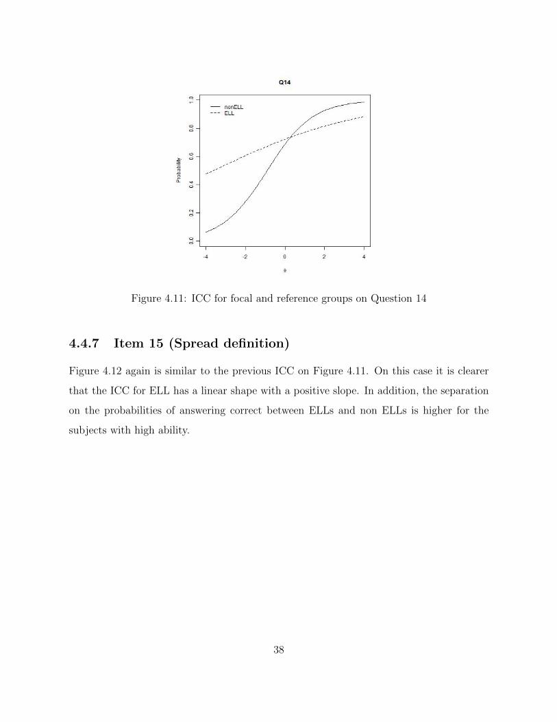
Figure 4.11: ICC for focal and reference groups on Question 14
4.4.7 Item 15 (Spread definition)
Figure 4.12 again is similar to the previous ICC on Figure 4.11. On this case it is clearer
that the ICC for ELL has a linear shape with a positive slope. In addition, the separation
on the probabilities of answering correct between ELLs and non ELLs is higher for the
subjects with high ability.
38
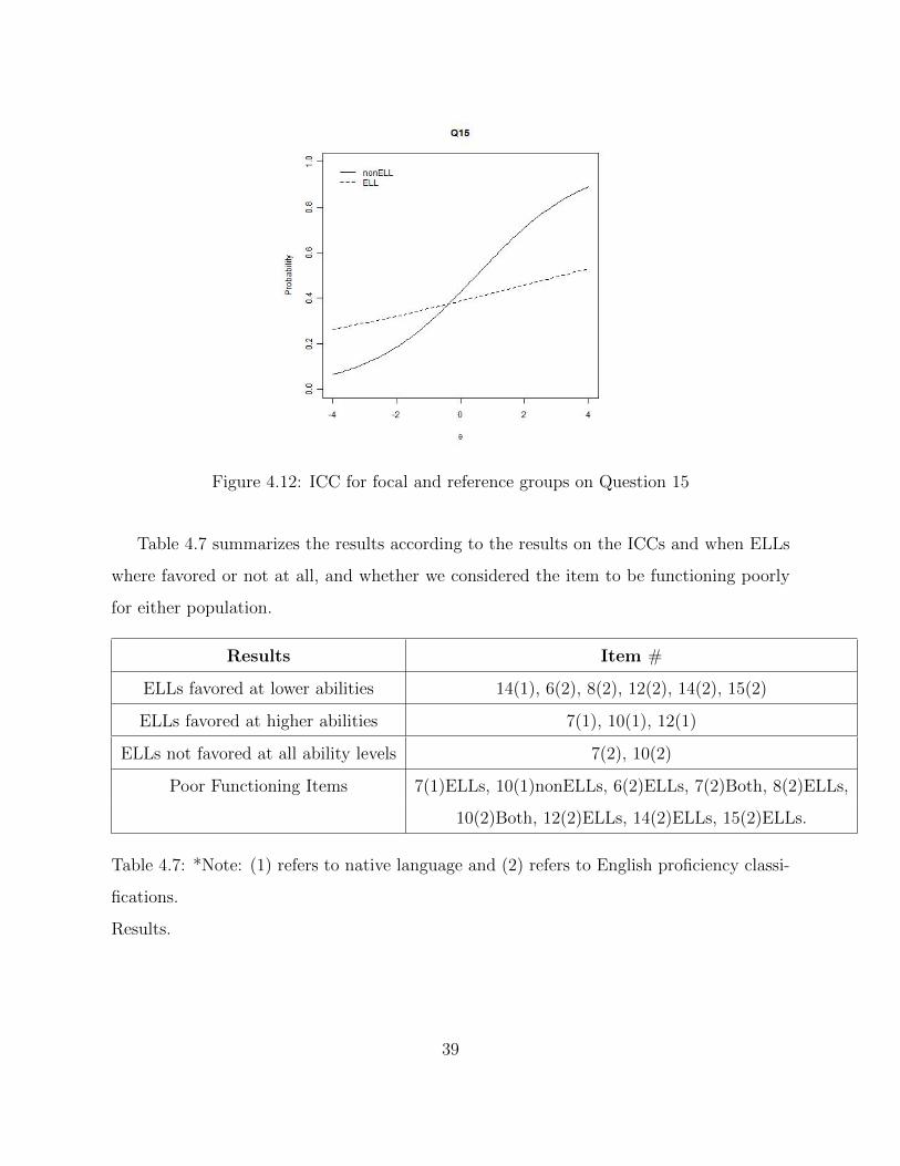
Figure 4.12: ICC for focal and reference groups on Question 15
Table 4.7 summarizes the results according to the results on the ICCs and when ELLs
where favored or not at all, and whether we considered the item to be functioning poorly
for either population.
Results Item #
ELLs favored at lower abilities 14(1), 6(2), 8(2), 12(2), 14(2), 15(2)
ELLs favored at higher abilities 7(1), 10(1), 12(1)
ELLs not favored at all ability levels 7(2), 10(2)
Poor Functioning Items 7(1)ELLs, 10(1)nonELLs, 6(2)ELLs, 7(2)Both, 8(2)ELLs,
10(2)Both, 12(2)ELLs, 14(2)ELLs, 15(2)ELLs.
Table 4.7: *Note: (1) refers to native language and (2) refers to English proficiency classi-
fications.
Results.
39
4.5 Analysis of the last 3 items
The last three items on the survey were not taken from the ARTIST items. We created
them to check whether there is a difference on the understanding of the context of the words
range, average, and spread among ELLs and nonELLs. If we recall Tables 4.3 and 4.4 show
the proportions of answers among ELLs and nonELLs for both classiffications respectively.
For item 13 we had a p-value of .1385 and .2605 for each classification respectively. For
item 14 we had a p-value of .5042 and .3677. For item 15 the p-value was .5301 and .2354.
As we can see the p-values are big on all items so at a significance level α = .05 we do not
reject the null hypothesis that the answer is independent of whether the respondant was
an ELL or nonELL for both classifications.
40
Chapter 5
Discussion
5.1 Individual Item Discussion
In the following, individual items are analyzed for DIF utilizing the ICCs. Only items
flagged for DIF are considered.
Item 6 (Average family size)
Item 6 was flagged as DIF on the second classification. They were given the total number
of households in a town and the average number of children per household and they were
asked to choose a true statement. If we recall from Table 4.4 for both ELLs and non-
ELLs the majority chose the correct answer b, with a higher percentage for non-ELLs
(43.8% compared to 38.8% for ELLs). The second modal answer for ELLs was c (The most
common number of children in a household is 2.2) with 28.3% and for non-ELLs the second
most common answer was a (Half the households in the town have more than 2 children).
This is perhaps due to a different understanding of the meaning of average for ELLs and
non-ELLs, where ELLs may be assuming the everyday meaning of average is common.
Additionally, ELLs also seem to be decontextualizing the answer from the context. That
is, it is reasonable to obtain a numerical mean of 2.2, but, in context, this does not imply
that the are 2.2 children on average on a household.
41
Item 7 (Income average)
For both classifications, Item 7 showed evidence of DIF. This item had skewed, mean,
median in the wording of the problem. For the first classification, the most common
answer was c for ELLs and non-ELLs when the correct answer was b. The percentages
for the correct answer are higher for non-ELLs on Table 4.3. It is likely that both groups
chose answer c (Not enough information to tell which is which) most often because they
didn’t understand the question and decided that the question couldn’t be answered with
the information given. For the second classification Table 4.4 shows that the percentages
are very close for both groups and the correct answer was chosen as many times by ELLs
than by non-ELLs.
Item 8 (Finding median after adding 5 to the top scores)
There was evidence of DIF on item 8 for the second classification only. The question
was about what would happen to the median if out of 100 students the 10 students with
the highest percentages were given a 5 point bonus. The majority of the subjects picked
incorrectly answer c which was that the median would be higher than the original. A
slightly higher percentage of non-ELsL chose the correct answer b compared to ELLs. This
is perhaps because both groups only have a computational understanding of the median so
since they were adding 5 points to the top 10% they thought that the median was going to
be higher. Perhaps ELLs yield the oncorrect answer more oftern thatn non-ELLs because
ELLs rely more on computational knowledge rather than contextual knowledge. If we recall
from the ICC plot on Figure 4.8 the ICC has a positive slope for ELLs meaning that the
better understanding they had of the concept of median the more likely they were going to
answer the item right.
42
Item 10 (Center and spread of a histogram)
Both classifications showed evidence of DIF for item 10. For this question respondents had
a histogram with some results and they were asked to answer which two measures were
most appropriate to describe center and spread for this distribution. Table 4.3 shows the
percentages for the first classification and it is evident that for both groups the most com-
mon answer was not the right answer. For ELLs the most common answer was d whereas
for non-ELLs it was b. Perhaps ELLs did not recognize the acronym for interquartile range
(IQR) that was in the correct answer c and they picked mean and standard deviation as
their answer. For non-ELLs it might be that mean and median are very common in statis-
tics so they choose that answer even though the question was asking for measures of center
and variation. On the second classification, the same happened, however, the percentages
are closer to each other that is why the ICCs are more similar on Figure 4.9.
Item 12 (Summarizing variability of a plot)
Both classifications flagged item 12 as DIF. On this case the correct answer was the third
most common answer by both groups on the first classifications. The modal answer for
ELLs was b and for non-ELLs was c. Both b and c would mean that the answer to
this item is standard deviation but for different reasons. Possibly ELLs choose b because
is a more general definition of standard deviation and reflects reliance on computational
knowledge. Perhaps they didn’t choose correctly interquartile range because they probably
didn’t contextualize the probelem by looking at the given histogram carefully to be able to
provide the correct answer.
Item 14 (Average definition)
Item 14 was a question about defining average. Both groups chose the correct answer which
was the statistical meaning of average. The second most common answer was d which
was giving a more general definition of average. It is important to note that more ELLs
43
answered d than non-ELLs. This is perhaps because ELLs might have less understanding
of the definition of average so the statistical meaning of average is harder for them. On the
second classification it is more evident the difference with a 26% for ELL against 18.9% for
non-ELLs answering d.
Item 15 (Spread definition)
This is a similar question to item 14 only with the definition of spread. Table 4.3 shows that
a higher percentage of ELLs chose answer a instead of the correct answer c. One reason
might be that most subjects were not familiar with the statistical meaning of spread, and
even more ELLs were unfamiliar with that definition. For the second classification, both
groups chose the incorrect answer a more than the correct answer c. Notice that the
percentage is higher between a and c for ELLs than for non-ELLs.
5.2 Limitations
The following describe the limitations associated with this study:
• Sample was smaller than anticipated. The target was to have at least 400 subjects
and we had 321 subjects. The reason might be due to time and resource constraints.
For one institution, we were only able to send email invitations to contact students,
which led to low response from students since students do not check their emails
regularly or the email might have been flagged as spam.
• For the last three questions, we were not specific in asking that we wanted the sta-
tistical meaning of the words.
• Item 12 had an acronym instead of the whole name, which might have confused the
subjects.
44
• Limited to Spanish speaking ELLs. Speakers of other languages were dropped from
the study since there were only 4; 1 German, 1 Korean, and 2 Hindi.
5.3 Conclusions and Recommendations for Teaching
There was some evidence of DIF on some items taken from the ARTIST database on
measures of center and variation. For some ability levels, ELLs had a lower probability
of answering the item correctly and for other levels of ability that probability was higher
for ELLs, depending on the type of question. Some items function poorly for one or both
populations. DIF items include those with a high level of technical vocabulary and those
where mistakes may easily be made if relying on computational knowledge rather than
contextualized interpretations. Overall, the questions that showed DIF were about mean,
median, interquartile range, spread, and average which are common terms that students
are expected to understand by the end of an introductory statistics course. Often, these
terms are hard to understand even for non-ELLs, but may be even more difficult for ELLs.
Students seemed to have issues when moving from the everyday language to the academic
language of the word. In addition, ELLs may have a different everyday register of a
word than non-ELLs which led them to answer differently. Table 5.1 provides teaching
recommendation supported by the findings of this study.
45
Recommendation Items Evidence
Use vocabulary activities 6, 8, 10, 14, 15 There is evidence of confusion between
(Lesser & Winsor, 2009) academic terms (mean and median) and also
between the everyday and academic use of words.
Emphasize context of 12 The explicit reference to the graphic
problem when teaching confused both populations and perhaps
(Lesser & Winsor, 2009) ELLs more so.
Introduce new ideas 8,12 ELLs had a good working knowledge
conceptually first so that of formulas without knowing how to
ELLs do not focus on properly apply them
procedural knowledge.
Make acronyms explicit 10 Many students may have been unable
to identify what the IQR was.
Emphasize difference 6, 14, 15 Students seemed to be confusing
between everyday and everyday meaning of average and spread
academic meaning of words with the academic meaning.
Emphasize meaning 10, 12 ELLs may have less familiarity
and use of statistical with using graphics due
graphics to academic background.
Table 5.1: Recommendations for teaching
46
References
[1] J. Abedi and C. Lord, “The Language Factor in Mathematics Tests,” Applied Mea-
surement in Education , 2001, 14(3) pp. 219–234.
[2] M. Aliaga, G. Cobb, C. Cuff, J. Garfield, R. Gould, R. Lock, T. Moore, A. Ross-
man, B. Stephenson, J. Utts, P. Velleman & J. Witmer Guidelines for Assessment
and Instruction in Statistics Education (GAISE) College Report, American Statistical
Association Alexandria, VA, 2010.
[3] D. August, M. Carlo, C. Dressler and C. Snow, “The Critical Role of Vocabulary De-
velopment for English Language Learners,” Learning Disabilities Research & Practice,,
20(1), 50-57 2005.
[4] C. L. Brown, “Equity of Literacy-Based Math Performance Assessments for English
Language Learners,” Bilingual Research Journal, 29(2), 2005, pp. 337–363.
[5] J. Cummins, “Language Proficiency, bilingualism, and academic achievement. In
P. A Richard Amato & M. A. Snow (eds.), ” The multicultural Classroom: Readings
for content area teachers, 1992, pp. 16–26, Reading, MA: Addison Wesley.
[6] R. J. de Ayala, The Theory and Practice of Item Response Theory, The Gilford Press,
New York, NY 2009.
[7] R. delMas, J. Garfield, A. Ooms, B. Chance “Assessing Students’ Conceptual Under-
standing After a First Course in Statistics,” Statistics Education Research Journal,
2006, 6(2).
[8] W. H. Finch and B. F. French, “Detection of Crossing Differential Item Functioning.
A Comparison of Four Methods.” Educational and Psychological Measurement, 2007,
67(565) pp. 565–582.
47
[9] S. M. Flores, J. Batalova, and M. Fix “The Educational Trajectories of English Lan-
guage Learners in Texas” Migration Policy Institute, Washington, DC, 2012.
[10] I. Gal and J. Garfield, “The Assessment Challenge in Statistics Education” IOS Press
1997.
[11] J. Garfield and I. Gal, “Assessment and statistics education: Current challenges and
directions.” International Statistical Review, 1999, 67(1) pp. 1–12.
[12] L. Garrison and J. K. Mora, “Adapting Mathematics Instruction for English-Language
Learners: The Language-Concept Connection,” In L. Ortiz-Franco, N. G. Hernandez,
& Y. De La Cruz (Eds.) Changing the Faces of Mathematics: Perspectives on Latinos,
National Council of Teachers of Mathematics. Reston, VA, 1999, pp. 35–48.
[13] C. Goldenberg, “Teaching English Language Learners: What the research does– and
does not –say,” American Educator, 33(2), 2008, pp. 8–44.
[14] M. D. Hidalgo, J. A. Lopez-Pina “Differential Item Functioning Detection and Effect
Size: A Comparison between Logistic Regression and Mantel-Haenszel Procedures,”
Educational and Psychological Measurement, 2004, 64(903) pp. 903-915.
[15] J. J. Kaplan, N. T. Rogness, D. G. Fisher, “Lexical Ambiguity: Making a Case
Against Spread,” Teaching Statistics, 34(2), 56–60, 2012.
[16] L. M. Lesser, M. S. Winsor, “English language learners in introductory statistics:
Lessons learned from an exploratory case study of two pre-service teachers.,” Statistics
Education Research Journal, 8(2), 5-32, 2009 pp. 5–32.
[17] L. M. Lesser, A. Wagler, A. Esquinca, and G. Valenzuela “Survey of Native English
Speakers and Spanish-Speaking English Language Learners in Tertiary Introductory
Statistics”
48
[18] K. Mahoney, “Linguistic Influences on Differential Item Functioning for Second Lan-
guage Learners on the National Assessment of Educational Progress” International
Journal of Testing, 8(1), 1990, pp. 14–33.
[19] A. J. Onwuegbuzie and N. L. Leech “Assessment in Statistics Courses: More than
a tool for evaluation”, Assessment & Evaluation in Higher Education,, 28(2), 2003,
pp. 115–127,.
[20] S. J. Osterlind and H. T. Everson, Differential Item Functioning, SAGE Publications,
Inc., Los Angeles, CA, 2009.
[21] D. R. Thompson and R. N. Rubenstein, “Learning Mathematics Vocabulary: Potential
Pitfalls and Instructional Strategies,” Mathematics Teacher, The National Council of
Teachers of Mathematics 93(7), 2000 pp. 568–574.
[22] W. J. van der Linden, R. K. Hambleton, Handbook of Modern Item Response Theory,
Springer, New York, NY, 1997.
[23] J. W. Young, S. Holtzman, J. Steinberg, “Score Comparability for Language Minority
Students on the Content Assessments Used by Two States,” (Research Report ETS
RR–11–27) Educational Testing Service, Princeton, NJ, 2011.
[24] B. D. Zumbo, “A Handbook on the Theory and Methods of Differential Item Func-
tioning (DIF): Logistic Regression Modeling as a Unitary Framework for Binary and
Likert-Type (Ordinal) Item Scores,” Directorate of Human Resources Research and
Evaluation, Department of National Defense, Ottawa, ON, 1999.
49

50
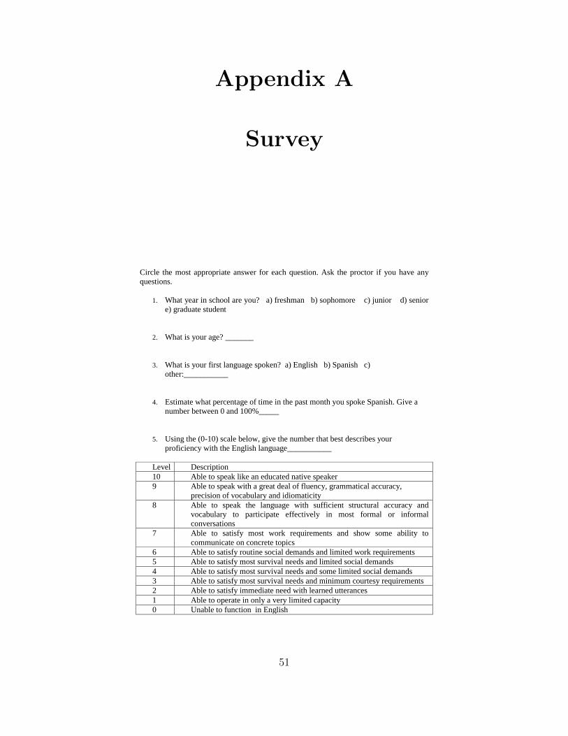
Appendix A
Survey
Circle the most appropriate answer for each question. Ask the proctor if you have any
questions.
1. What year in school are you? a) freshman b) sophomore c) junior d) senior
e) graduate student
2. What is your age? _______
3. What is your first language spoken? a) English b) Spanish c)
other:___________
4. Estimate what percentage of time in the past month you spoke Spanish. Give a
number between 0 and 100%_____
5. Using the (0-10) scale below, give the number that best describes your
proficiency with the English language___________
Level Description
10 Able to speak like an educated native speaker
9 Able to speak with a great deal of fluency, grammatical accuracy,
precision of vocabulary and idiomaticity
8 Able to speak the language with sufficient structural accuracy and
vocabulary to participate effectively in most formal or informal
conversations
7 Able to satisfy most work requirements and show some ability to
communicate on concrete topics
6 Able to satisfy routine social demands and limited work requirements
5 Able to satisfy most survival needs and limited social demands
4 Able to satisfy most survival needs and some limited social demands
3 Able to satisfy most survival needs and minimum courtesy requirements
2 Able to satisfy immediate need with learned utterances
1 Able to operate in only a very limited capacity
0 Unable to function in English
51
6. The school committee of a small town wanted to determine the average number of children
per household in their town. They divided the total number of children in the town by 50, the
total number of households. Which of the following statements must be true if the average
children per household are 2.2 children?
a. Half the households in the town have more than 2 children.
b. There are a total of 110 children in the town.
c. The most common number of children in a household is 2.2.
d. None of the above.
7. The distribution of the top 1% of individual incomes in the US is strongly skewed to the
right. In 1997, the two measures of center for the top 1% of individual incomes were
$330,000 and $675,000. Which number represents the mean income of the top1% and which
number represents the median income of the top 1%? Choose the best answer.
a. $330,000 is the mean and $675,000 is the median.
b. $330,000 is the median and $675,000 is the mean.
c. Not enough information to tell which is which.
8. You give a test to 100 students and determine the median score. After grading the test, you
realize that the 10 students with the highest scores did exceptionally well. You decide to
award these 10 students a bonus of 5 more points. The median of the new score distribution
will be ___________ that of the original score distribution.
a. lower than
b. equal to
c. higher than
d. depending on skewness, higher or lower than
9. Find the range of the following list: 32, 36, 48, 49, 50, 53, 54, 56, 60, 62
a. 62
b. 5
c. 10
d. 30
52
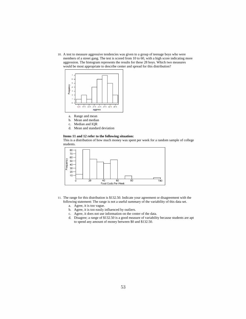
10. A test to measure aggressive tendencies was given to a group of teenage boys who were
members of a street gang. The test is scored from 10 to 60, with a high score indicating more
aggression. The histogram represents the results for these 28 boys. Which two measures
would be most appropriate to describe center and spread for this distribution?
a. Range and mean
b. Mean and median
c. Median and IQR
d. Mean and standard deviation
Items 11 and 12 refer to the following situation:
This is a distribution of how much money was spent per week for a random sample of college
students.
11. The range for this distribution is $132.50. Indicate your agreement or disagreement with the
following statement: The range is not a useful summary of the variability of this data set.
a. Agree, it is too vague.
b. Agree, it is too easily influenced by outliers.
c. Agree, it does not use information on the center of the data.
d. Disagree; a range of $132.50 is a good measure of variability because students are apt
to spend any amount of money between $0 and $132.50.
53

12. What is the best measure to use to summarize the variability of this data set?
a. Range, because it tells you the overall spread of the data.
b. Standard deviation, because it is based on all the information in the data set.
c. Standard deviation, because it is the most commonly used measure of variability.
d. Interquartile range, because it is resistant to outliers.
13. Range is defined as:
a. The set of all output values produced by a function.
b. The difference between the highest and the lowest values in a set.
c. The numbered place in the list of ordered values.
d. The size of a data set.
e. The distance a charged particle travels before stopping
f. The set of notes a musical instrument can play, or that are used in a piece of music
14. Average is defined as:
a. Ordinary, Normal, typical, mediocre, not extraordinary, common, neither outstanding
nor poor, standard
b. Mean
c. Median or in the middle
d. Overall summary on something, general value that represents most of the data,
overall outcome
e. Mode, most common number
f. Majority
g. A value we can use to compare one person’s performance to the group
15. Spread is defined as:
a. To scatter distribute, disperse; to go apart or separate; to extend over a larger space
b. To distribute in a thin layer, smear or cover evenly
c. Range or difference between two numbers as in point spread
d. Extend, open out as in spread his wings
e. Butter, jam, dip
f. Spreadsheet
g. A large group
h. Graph
54
Page 1 of 3
University of Texas at El Paso (UTEP) Institutional Review Board Informed Consent Form for Research Involving Human Subjects
Protocol Title: Analysis of Differential Item Functioning on measures of center and variation for
ELL and non-ELL students.
Principal Investigator: Angelica Monarrez and Amy Wagler
UTEP: Mathematical Sciences Department
1. Introduction
You are being asked to participate in the research project described below. Before agreeing to
take part in this research study, it is important that you read the consent form that describes the
study. Please ask the study researcher or the study staff to explain any words or information
that you do not clearly understand.
2. Why is this study being done?
You have been asked to take part in a research study about how communication and language
affect learning statistics in an introductory statistic class. The main purpose of this study is to
understand better what strengths and difficulties students have with language and learning
measures of center and variation in an introductory statistics course. You are being asked to be
in the study because you were registered in an introductory statistics class this past semester. If
you decide to participate in this study, your involvement will last about approximately 5-8
minutes.
3. What is involved in the study?
If you agree to take part in this study, you will be asked to answer a short survey. The
responses are anonymous and cannot be traced to the participant.
4. What are the risks and discomforts of the study?
There are no known risks associated with this research.
Page 2 of 3
5. Are there benefits to taking part in this study?
There will be no direct benefits to you for taking part in this study. Participating in this study may
help you reflect upon or notice some details about your own process on learning in an online
statistics class. This research may help the researchers understand what difficulties students
face in a statistics class so that more effective teaching strategies can be developed for future
students.
6. What other options are there?
Participation in this study is optional. There will be no penalties involved if you choose not to
take part in this study. We hope, of course, that you will choose to participate because your
participation will make the study stronger.
7. Who is paying for this study?
This study does not receive funding from any association.
8. What are my costs?
There are no costs to you beyond the time you spend on the survey.
9. Will I be paid to participate in this study?
You will not be paid for taking part in this research study.
10. What if I want to withdraw, or am asked to withdraw from this study?
Taking part in this study is voluntary. You have the right to choose not to take part in this
study. If you do not take part in the study, there will be no penalty. If you choose to take
part, you have the right to stop at any time. If you do stop, we encourage you to talk to a
member of the research group so that they know why you are leaving the study.

Page 3 of 3
11. Who do I call if I have questions or problems?
You may ask any questions you have now. If you have questions later, you may contact Dr.
Amy Wagler (915-747-6847; [email protected]). If you have questions or concerns about
your participation as a research subject, you may contact the UTEP Institutional Review
Board (IRB) at (915-747-8841) or [email protected].
12. What about confidentiality?
1. Your part in this study is anonymous. You are not providing your name on the survey and
any results will be reported (at meetings or in publications) in a manner where no individual
can be identified.
2. Every effort will be made to keep your information confidential, unless disclosure is
required by law. Organizations that may inspect and/or copy your research records for
quality assurance and data analysis include, but are not necessarily limited to:
• The sponsor or an agent for the sponsor
• Department of Health and Human Services
• UTEP Institutional Review Board
13. Authorization Statement I have read each page of this paper about the study (or it was read to me). I know that being
in this study is voluntary and I choose to be in this study. I know I can stop being in this
study without penalty. I can get a copy of this consent form now and can get information on
results of the study later if I wish.
Participant Name: Date:
Participant Signature: Time:
Consent form explained/witnessed by:
Signature
Printed name:
Date: Time:
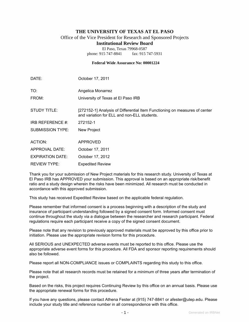
- 1 - Generated on IRBNet
THE UNIVERSITY OF TEXAS AT EL PASOOffice of the Vice President for Research and Sponsored Projects
Institutional Review BoardEl Paso, Texas 79968-0587
phone: 915 747-8841 fax: 915 747-5931
Federal Wide Assurance No: 00001224
DATE: October 17, 2011 TO: Angelica Monarrez
FROM: University of Texas at El Paso IRB STUDY TITLE: [272152-1] Analysis of Differential Item Functioning on measures of center
and variation for ELL and non-ELL students.
IRB REFERENCE #: 272152-1
SUBMISSION TYPE: New Project ACTION: APPROVED
APPROVAL DATE: October 17, 2011
EXPIRATION DATE: October 17, 2012
REVIEW TYPE: Expedited Review
Thank you for your submission of New Project materials for this research study. University of Texas atEl Paso IRB has APPROVED your submission. This approval is based on an appropriate risk/benefitratio and a study design wherein the risks have been minimized. All research must be conducted inaccordance with this approved submission.
This study has received Expedited Review based on the applicable federal regulation.
Please remember that informed consent is a process beginning with a description of the study andinsurance of participant understanding followed by a signed consent form. Informed consent mustcontinue throughout the study via a dialogue between the researcher and research participant. Federalregulations require each participant receive a copy of the signed consent document.
Please note that any revision to previously approved materials must be approved by this office prior toinitiation. Please use the appropriate revision forms for this procedure.
All SERIOUS and UNEXPECTED adverse events must be reported to this office. Please use theappropriate adverse event forms for this procedure. All FDA and sponsor reporting requirements shouldalso be followed.
Please report all NON-COMPLIANCE issues or COMPLAINTS regarding this study to this office.
Please note that all research records must be retained for a minimum of three years after termination ofthe project.
Based on the risks, this project requires Continuing Review by this office on an annual basis. Please usethe appropriate renewal forms for this procedure.
If you have any questions, please contact Athena Fester at (915) 747-8841 or [email protected]. Pleaseinclude your study title and reference number in all correspondence with this office.
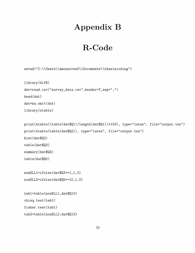
Appendix B
R-Code
setwd("C:\\Users\\amonarrez5\\Documents\\thesiscoding")
library(difR)
dat=read.csv("survey_data.csv",header=T,sep=",")
head(dat)
dat=na.omit(dat)
library(xtable)
print(xtable((table(dat$Q1)/length(dat$Q1))*100), type="latex", file="output.tex")
print(xtable(table(dat$Q2)), type="latex", file="output.tex")
hist(dat$Q2)
table(dat$Q3)
summary(dat$Q4)
table(dat$Q5)
nonELL1=ifelse(dat$Q3==1,1,0)
nonELL2=ifelse(dat$Q5==10,1,0)
tab1=table(nonELL1,dat$Q13)
chisq.test(tab1)
fisher.test(tab1)
tab2=table(nonELL2,dat$Q13)
59
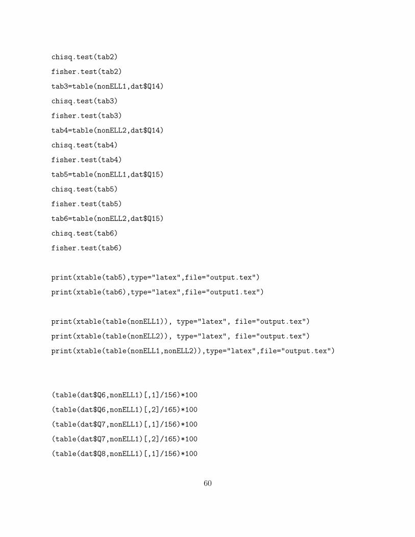
chisq.test(tab2)
fisher.test(tab2)
tab3=table(nonELL1,dat$Q14)
chisq.test(tab3)
fisher.test(tab3)
tab4=table(nonELL2,dat$Q14)
chisq.test(tab4)
fisher.test(tab4)
tab5=table(nonELL1,dat$Q15)
chisq.test(tab5)
fisher.test(tab5)
tab6=table(nonELL2,dat$Q15)
chisq.test(tab6)
fisher.test(tab6)
print(xtable(tab5),type="latex",file="output.tex")
print(xtable(tab6),type="latex",file="output1.tex")
print(xtable(table(nonELL1)), type="latex", file="output.tex")
print(xtable(table(nonELL2)), type="latex", file="output.tex")
print(xtable(table(nonELL1,nonELL2)),type="latex",file="output.tex")
(table(dat$Q6,nonELL1)[,1]/156)*100
(table(dat$Q6,nonELL1)[,2]/165)*100
(table(dat$Q7,nonELL1)[,1]/156)*100
(table(dat$Q7,nonELL1)[,2]/165)*100
(table(dat$Q8,nonELL1)[,1]/156)*100
60
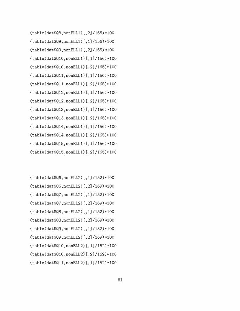
(table(dat$Q8,nonELL1)[,2]/165)*100
(table(dat$Q9,nonELL1)[,1]/156)*100
(table(dat$Q9,nonELL1)[,2]/165)*100
(table(dat$Q10,nonELL1)[,1]/156)*100
(table(dat$Q10,nonELL1)[,2]/165)*100
(table(dat$Q11,nonELL1)[,1]/156)*100
(table(dat$Q11,nonELL1)[,2]/165)*100
(table(dat$Q12,nonELL1)[,1]/156)*100
(table(dat$Q12,nonELL1)[,2]/165)*100
(table(dat$Q13,nonELL1)[,1]/156)*100
(table(dat$Q13,nonELL1)[,2]/165)*100
(table(dat$Q14,nonELL1)[,1]/156)*100
(table(dat$Q14,nonELL1)[,2]/165)*100
(table(dat$Q15,nonELL1)[,1]/156)*100
(table(dat$Q15,nonELL1)[,2]/165)*100
(table(dat$Q6,nonELL2)[,1]/152)*100
(table(dat$Q6,nonELL2)[,2]/169)*100
(table(dat$Q7,nonELL2)[,1]/152)*100
(table(dat$Q7,nonELL2)[,2]/169)*100
(table(dat$Q8,nonELL2)[,1]/152)*100
(table(dat$Q8,nonELL2)[,2]/169)*100
(table(dat$Q9,nonELL2)[,1]/152)*100
(table(dat$Q9,nonELL2)[,2]/169)*100
(table(dat$Q10,nonELL2)[,1]/152)*100
(table(dat$Q10,nonELL2)[,2]/169)*100
(table(dat$Q11,nonELL2)[,1]/152)*100
61
(table(dat$Q11,nonELL2)[,2]/169)*100
(table(dat$Q12,nonELL2)[,1]/152)*100
(table(dat$Q12,nonELL2)[,2]/169)*100
(table(dat$Q13,nonELL2)[,1]/152)*100
(table(dat$Q13,nonELL2)[,2]/169)*100
(table(dat$Q14,nonELL2)[,1]/152)*100
(table(dat$Q14,nonELL2)[,2]/169)*100
(table(dat$Q15,nonELL2)[,1]/152)*100
(table(dat$Q15,nonELL2)[,2]/169)*100
dat[,6]=ifelse(dat$Q6==2,1,0)
dat[,7]=ifelse(dat$Q7==2,1,0)
dat[,8]=ifelse(dat$Q8==2,1,0)
dat[,9]=ifelse(dat$Q9==4,1,0)
dat[,10]=ifelse(dat$Q10==3,1,0)
dat[,11]=ifelse(dat$Q11==2,1,0)
dat[,12]=ifelse(dat$Q12==4,1,0)
dat[,13]=ifelse(dat$Q13==2,1,0)
dat[,14]=ifelse(dat$Q14==2,1,0)
dat[,15]=ifelse(dat$Q15==3,1,0)
items=dat[,6:15]
items1=data.frame(items,nonELL1)
dicho.uDIF=dichoDif(items1,group="nonELL1",focal.name=0,
method=c("TID","MH","Std","Logistic","BD","Lord","Raju","LRT"),
save.output=T,output=c("out","default"),alpha=.1,type="udif")
62

dicho.nuDIF=dichoDif(items1,group="nonELL1",focal.name=0,
method=c("TID","MH","Std","Logistic","BD","Lord","Raju","LRT"),
save.output=T,output=c("out1","default"),alpha=.1,type="nudif")
(dif1.Lord=difLord(items1, group="nonELL1",model="2PL", focal.name=0,
save.output=T,output=c("out4","default"),alpha=.1))
items2=data.frame(items,nonELL2)
dif2.Lord=difLord(items2, group="nonELL2",model="2PL", focal.name=0,
save.output=T,output=c("out4","default"),alpha=.1)
dicho.uDIF2=dichoDif(items2,group="nonELL2",focal.name=0,
method=c("TID","MH","Std","Logistic","BD","Lord","Raju","LRT"),
save.output=T,output=c("out6","default"),alpha=.1,type="udif")
dicho.nuDIF2=dichoDif(items2,group="nonELL2",focal.name=0,
method=c("TID","MH","Std","Logistic","BD","Lord","Raju","LRT"),
save.output=T,output=c("out7","default"),alpha=.1,type="nudif")
print(xtable(dicho.uDIF2$DIF),type="latex",output="output2.tex")
print(xtable(dicho.nuDIF2$DIF),type="latex",output="output2.tex")
print(xtable(dicho.uDIF$DIF),type="latex",output="output2.tex")
print(xtable(dicho.nuDIF$DIF),type="latex",output="output2.tex")
plot(dif1.Lord,plot="itemCurve",item=2,save.plot=TRUE,
save.options=c("plot24","default","jpeg"),group.names=c("nonELL","ELL"))
plot(dif1.Lord,plot="itemCurve",item=5,save.plot=TRUE,
save.options=c("plot25","default","jpeg"),group.names=c("nonELL","ELL"))
plot(dif1.Lord,plot="itemCurve",item=7,save.plot=TRUE,
save.options=c("plot26","default","jpeg"),group.names=c("nonELL","ELL"))
63
plot(dif1.Lord,plot="itemCurve",item=9,save.plot=TRUE,
save.options=c("plot27","default","jpeg"),group.names=c("nonELL","ELL"))
plot(dif2.Lord,plot="itemCurve",item=1,save.plot=TRUE,
save.options=c("plot28","default","jpeg"),group.names=c("nonELL","ELL"))
plot(dif2.Lord,plot="itemCurve",item=2,save.plot=TRUE,
save.options=c("plot29","default","jpeg"),group.names=c("nonELL","ELL"))
plot(dif2.Lord,plot="itemCurve",item=3,save.plot=TRUE,
save.options=c("plot30","default","jpeg"),group.names=c("nonELL","ELL"))
plot(dif2.Lord,plot="itemCurve",item=5,save.plot=TRUE,
save.options=c("plot31","default","jpeg"),group.names=c("nonELL","ELL"))
plot(dif2.Lord,plot="itemCurve",item=7,save.plot=TRUE,
save.options=c("plot32","default","jpeg"),group.names=c("nonELL","ELL"))
plot(dif2.Lord,plot="itemCurve",item=9,save.plot=TRUE,
save.options=c("plot33","default","jpeg"),group.names=c("nonELL","ELL"))
plot(dif2.Lord,plot="itemCurve",item=10,save.plot=TRUE,
save.options=c("plot34","default","jpeg"),group.names=c("nonELL","ELL"))
64
Curriculum Vitae
Angelica Monarrez was born on December 9, 1985, in Juarez, Chihuahua, Mexico. She is
the last daughter of Rodolfo and Ana Monarrez, she graduated from Colegio de Bachilleres
High School in 2004. She then entered the Autonomous University of Ciudad Juarez in
hopes of pursuing a degree in Mathematics, she later transfer to The University of Texas
at El Paso in 2006. In 2010 she succeeded her goal and received a bachelors in science.
However, in the process of pursuing her degree she became interested in Statistics. It was
then that she decided to focus all of her attention to the study of Statistics. Soon after
graduation she was admitted in the Masters program in Statistics at The University of
Texas at El Paso.
During her time as an undergraduate she worked as a tutor in mathematics as well as
a peer leader for Pre-Calculus and Calculus courses. Later as a graduate student, she was
a research assistant on the implementation of supplemental instruction for Pre-Calculus at
El Paso Community College. She also worked as a teacher assistant on her last year as a
master student. Her jobs have helped her realize the strong passion she has for teaching
and research. After graduading Angelica plans to take her two passions and pursue her
doctoral studies in math education.
Permanent address: 200 North Mesa Hills Apt # 1007
El Paso, Texas 79912
65


![Running Head: DIFFERENTIAL ITEM FUNCTIONING OF THE SRQ …timo.gnambs.at/sites/default/files/gnambs+hanfstingl2013.pdf · DIF OF THE SRQ-A[G] 3 A Differential Item Functioning Analysis](https://img.pdfslide.us/doc/110x75/5b89a81a7f8b9a655f8cae19/running-head-differential-item-functioning-of-the-srq-timo-hanfstingl2013pdf.jpg)