A STEP-WISE METHOD FOR EVALUATION OF DIFFERENTIAL ITEM FUNCTIONING …issue-2/pdfs/3_khalid.pdf · A STEP-WISE METHOD FOR EVALUATION OF DIFFERENTIAL ITEM FUNCTIONING Muhammad Naveed

Quantitative Methods Inquires

25

A STEP-WISE METHOD FOR EVALUATION OF DIFFERENTIAL ITEM FUNCTIONING

Muhammad Naveed KHALID University of Cambridge ESOL Examinations, UK E-mail: [email protected]

Cees A. W. GLAS PhD, University Professor, Department of Research Methodology, Measurement and Data Analysis Faculty of Behavioral Science, University of Twente, Netherlands E-mail: [email protected]

Abstract: Item bias or differential item functioning (DIF) has an important impact on the fairness of psychological and educational testing. In this paper, DIF is seen as a lack of fit to an item response (IRT) model. Inferences about the presence and importance of DIF require a process of so-called test purification where items with DIF are identified using statistical tests and DIF is modeled using group-specific item parameters. In the present study, DIF is identified using item-oriented Lagrange multiplier statistics. The first problem addressed is that the dependence of these statistics might cause problems in the presence of a relatively large number DIF items. A stepwise procedure is proposed where DIF items are identified one or two at a time. Simulation studies are presented to illustrate the power and Type I error rate of the procedure. The second problem pertains to the importance of DIF, i.e., the effect size, and related problem of defining a stopping rule for the searching procedure for DIF. The estimate of the difference between the means and variances of the ability distributions of the studied groups of respondents is used as an effect size and the purification procedure is stopped when the change in this effect size becomes negligible. Key words: Differential Item Functioning; Effect Size; Item Response Theory; Model Fit; Polytomous Items

INTRODUCTION

Differential item functioning (DIF) occurs when respondents with the same ability but from different groups (say, gender or ethnicity groups) have a different response probabilities on an item of a test or questionnaire (Embretson & Reise, 2000). Several statistical DIF detection methods have emerged in the last three decades (Camilli, 1992; Dorans & Kulick 1986; Finch, 2005; Holland & Thayer, 1988; Kelderman & Macready, 1990; Lord, 1980; Muthén, 1988; Shealy & Stout, 1993; Swaminathan & Rogers, 1990; Thissen, Steinberg, & Wainer, 1988; Raju, 1988; Roussos & Stout, 1996). During this period many researchers have reviewed various DIF detection methods (e.g., Camilli & Shepard, 1994; Holland & Wainer, 1993; Millsap & Everson, 1993; Penfield & Camilli, 2007; Roussos &


26

Stout, 2004). Most of the techniques proposed for the detection of DIF have been based on the evaluation of differences in response probabilities between groups conditional on some measure of ability. We can classify these techniques under two general categories: the first category is where a manifest score, such as the number-correct score, is taken as a proxy for ability and the second is where a latent ability variable of an IRT model functions as an ability measure. The most common method used in the first category is the Mantel-Haenszel (MH) approach where DIF is evaluated by testing whether the response probability, given number-correct scores, differs between the groups. The MH test works quite well in practice under the Rasch model. Fischer (1993, 1995), however, argues that its application under other IRT models raises several theoretical limitations. For instance, sufficient statistics does not hold for the 2PL and 3PL models. Fischer’s view on sufficient statistics equally applies to the log-linear approach where sum scores are used as proxies for ability; this view is also shared by Meredith and Millsap (1992). The observed score is nonlinearly related to the latent ability metric (Embretson & Reise, 2000; Lord, 1980) and factors such as guessing may preclude an adequate representation of the probability of correct response conditional on ability. Having said that, in general the correlation between the number-correct scores and ability estimates is quite high, so this is not the most important reason for considering alternative methods. The main problem arises in situations where the number-correct score loses its value as a proxy for ability. For example, there are test situations with large amounts of missing data and in the case of computer adaptive testing, where every student is administered a virtually unique set of items. In all these situations the number-correct score may not be appropriate for a meaningful assessment.

In an IRT model, ability is represented by latent variable θ, and a possible solution to the number correct score problem is to apply the MH and log-linear approach using subgroups that are homogenous with respect to an estimate of θ. This, however, introduces a different problem that the estimate of θ is subject to estimation error, which is difficult to take into account when forming the subgroups. An alternative is to view DIF as a special case of misfit of an IRT model and to use the machinery for IRT model-fit evaluation to explore DIF. An overview of this approach was given by Thissen, Steinberg, and Wainer (1993). In that overview, evaluation of item parameter invariance over subgroups using Likelihood ratio and Wald statistics was presented as the main statistical tool for detection of DIF. Glas (1998, 1999) argues that the Likelihood ratio and Wald approach are not very efficient because they require estimation of the parameters of the IRT model under the alternative hypothesis of DIF for every single item. To address these shortcomings, Glas (1998, 1999) proposes using the Lagrange multiplier (LM) test by Aitchison and Silvey (1958), and the equivalent efficient-score test (Rao, 1948), which do not require estimation of the parameters of the alternative model. Further, this approach supports the evaluation of many more model assumptions such as the form of the response function, unidimensionality and local stochastic independence, both at the level of items (Glas & Falcón, 2003) and at the level of persons (Glas & Dagohoy, 2007).

All methods listed above are seriously affected by the presence of high proportions of DIF items in a test and by the inclusion of DIF items in matching variable. To address this issue, several scale purification procedures have been suggested for the DIF detection methods, such as the two-stage or iterative Mantel-Haenszel method (Holland & Thayer, 1988), the iterative Mantel method, the iterative generalized Mantel-Haenszel method


27

(Wang & Su, 2004a, 2004b), the iterative logistic regression method (French & Maller, 2007), and the iterative linking IRT-based method (Candell & Drasgow, 1988; Park & Lautenschlager, 1990).

Scale purification procedures are useful in maintaining Type I error rate and have high power when tests contain only a few DIF items. However, if tests have many DIF items, then DIF contamination cannot be completely eliminated by current scale purification procedures. Similar conclusions have been drawn when scale purification procedures were implemented on IRT-based DIF methods (Candell & Drasgow, 1988; Lautenschlager, Flaherty, & Park, 1994; Park & Lautenschlager, 1990) and non-IRT-based DIF methods (Clauser, Mazor, & Hambleton, 1993; French & Maller, 2007; Hidalgo-Montesinos & Gómez-Benito, 2003; Holland & Thayer, 1988; Miller & Oshima, 1992; Navas-Ara & Gómez-Benito, 2002; Wang & Su, 2004a, 2004b, 2010). In this paper we propose an alternative scale purification method using Lagrange multiplier tests to address DIF contamination.

The significance of DIF, the extent to which the inferences made using test results are biased by DIF, is yet another important issue that needs to be looked at. The effect size of DIF is important to consider to avoid complicating inferences by practically trivial but statistically significant results. An example of a method to quantify the effect size is the DIF classification system for use with the MH statistical method developed by the Educational Testing Service (Camilli & Shepard, 1994; Clauser & Mazor, 1998). In an IRT framework we propose to use an estimate of the difference between the means of the ability distributions of the studied groups of respondents as an effect size. This is motivated by the fact that ability distributions play an important role in most inferences made using IRT, such as in making pass/fail decisions, test equating, and the estimation of linear regression models on ability parameters as used in large scale education surveys such as NEAP, TIMSS and PISA.

In this paper we would first sketch a model of DIF and a concise framework of Lagrange multiplier test for the identification of DIF items. We would then present a number of simulation studies of the Type I error rate and power analysis. The difference between two versions of the LM test, one targeted at uniform DIF and one targeted at non-uniform DIF will be shown using a simulated example. This is followed by presenting an example using empirical data to show how the procedure works in practice. Finally, some conclusions are drawn, and suggestions for further research are provided.

DETECTION AND MODELING OF DIF

In IRT models, the influences of items and persons on the observed responses are modeled by different sets of parameters. Since DIF is defined as the occurrence of differences in expected scores conditional on ability, IRT modeling seems especially fit for dealing with this problem. In practice, more than one DIF item may be present and therefore a stepwise procedure will be proposed where DIF items are identified one or two at a time. Both the significance of the test statistics and the impact of DIF are taken into account. The following procedure will be used here for detection and modeling of DIF. First, marginal maximum likelihood (MML) estimates of the item parameters and the means and variance parameters of the different groups of respondents are made using all items. Then an item is identified with the largest significant value on a Lagrange multiplier (LM) test statistic targeted at DIF. To model the DIF in this item, the item is given group-specific item


28

parameters. That is, in the analysis, the item is split into two virtual items, one that is supposed to be given to the focal group and one that is supposed to be given to the reference group. Then, new MML estimates are made and the impact of DIF in terms of the change in the means and variances of the ability distributions is evaluated. If this change is considered substantial, the next item with DIF is searched for. The process is repeated until no more significant or relevant DIF is found. The assumptions of this procedure are that (1) the item which is mostly affected by DIF will have the largest value of the LM statistic regardless of the bias caused by the other items with DIF, and (2) the change in the means and variances of ability distributions will decrease when the items with the DIF are given group specific item parameters one or two at a time. IRT Models

In the present study, we both consider dichotomously and polytomously scored items. For dichotomously scored items, the one-parameter logistic model (1PLM) by Rasch (1960), the two-parameter logistic model (2PLM) and the three-parameter logistic model (3PLM) by Birnbaum (1968) will be used. For polytomously scored items, we use the generalized partial credit model (GPCM, Muraki, 1992). However, the methods proposed here also apply to other models for polytomously scored items, such as the PCM by Masters (1982) or the nominal response model by Bock (1972).

In the 3PLM, the item is characterized by a difficulty parameter i , a discrimination

parameter i and a guessing parameter i . Further, θn is the latent ability parameter of

respondent n. The probability of correctly answering an item (denoted by X 1ni ) is given

by

exp( ( ))

( X 1 | ) ( ) (1 ) .1 exp( ( ))ni n i i

i n ii n

i n i

P P

(1)

If the guessing parameter i is constrained to zero, the model reduces to the 2PLM

and if the discrimination parameter i is also constrained to one, the model reduces to the

1PLM. DIF pertains to different response probabilities in different groups. Here we consider

two groups labeled the reference group and the focal group. The generalization to more than two groups is straightforward. A background variable will be defined by

1 if person n belongs to the focal group,

0 if person n belongs to the reference group.ny

As a generalization of the model defined by equation 1 we consider

exp( ( ) ( ( )))

( ) (1 ) .1 exp( ( ) ( ( )))i i

i n i n i n ii n

i n i n i n i

yP

y

(2)

This model implies that the responses of the reference population are properly

described by the model given by equation 1, but that the responses of the focal population


29

need additional location parameters i , additional discrimination parameters i , or both as

given by equation 2. The first instance covers so-called uniform DIF, that is, a shift of the item response curve for the focal population, while the later two cases are often labeled non-uniform DIF, that is, the item response curve for the focal population is not only shifted, but it also intersects the item response curve of the reference population.

For polytomous items, the GPCM by Muraki (1992) will be used. The probability of a

student n scoring in category j on item i (denoted by X 1nij ) is given by

1

exp( )( X 1 | ) ( ) ,

1 exp( )i

i n ijnij n ij n M

i n ihh

jP P

h

(3)

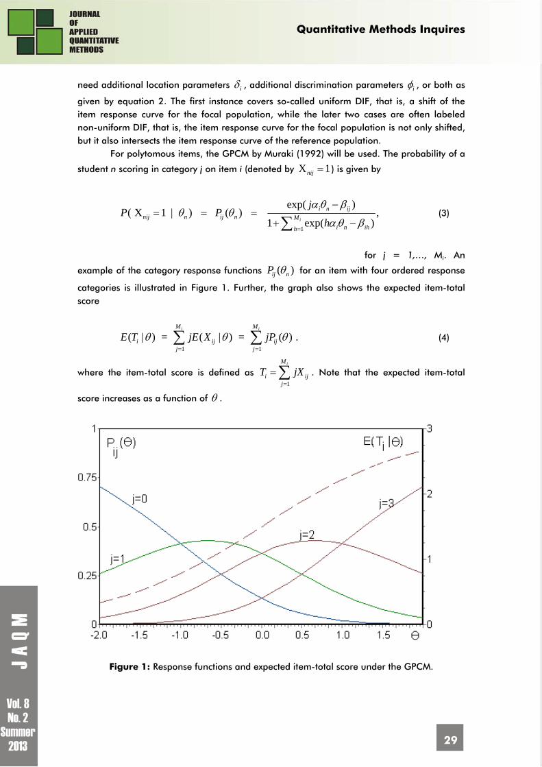
for j = 1,…, Mi. An

example of the category response functions ( ) ij nP for an item with four ordered response

categories is illustrated in Figure 1. Further, the graph also shows the expected item-total score

1 1

( | ) = ( | ) = ( ) .i iM M

i ij ijj j

E T jE X jP (4)

where the item-total score is defined as 1

iM

i ijj

T jX

. Note that the expected item-total

score increases as a function of .

Figure 1: Response functions and expected item-total score under the GPCM.


30

MML Estimation The LM test for DIF will be implemented in an MML estimation framework. To

describe the statistic, MML estimation will be outlined first. MML estimation was developed

by Bock and Aitkin (1981; see also Bock & Zimowski, 1997; Mislevy, 1984, 1986; Rigdon &

Tsutakawa, 1983). In the MML framework adopted here, it is assumed that the respondents

belong to groups, and that ability parameters of the respondents within a group have a

normal distribution indexed by a group specific-mean and variance parameter. Let

( )( ; )n y ng λ be the density of ability distribution of group y, with parameters ( )y nλ where

y(n) = yn, i.e., the index of the group to which respondent n belongs. To identify the model,

the mean and variance of one of the groups are usually set to zero and unity, respectively.

Further, let ξ be a vector that contains all the item parameters. Finally, η is the vector of all

item parameters ξ and the parameters λ of the ability distributions. The log likelihood

function of η can be written as

( )1

) log ( | , ) ( ; ) .log (N

n n y nn

n np g dL

η x ξ λ (5)

where ( | , )n np x ξ is the probability of response pattern xn of respondent n (n = 1,…, N).

The estimation equations that maximize the log-likelihood are found by setting the first-order derivatives of equation 5 with respect to η equal to zero. Glas (1999) shows that expressions for the first-order derivatives can be derived using Fischer’s identity (Efron, 1977; Louis, 1982):

log ( ) ( ) | ;n nn

L E

η η xη

(6)

with

( )( ) log ( | , ) ( ; )n n n y nnp g η x ξ

ηλ

The expectation in equation 6 is with respect to the posterior

distribution ( )( | ; , )n n y np x ξ . That is, the first order derivatives are equal to the posterior

expectations of the first order derivatives of a likelihood function where the ability parameters are treated as observations. This grossly simplifies the derivations of the

likelihood equations because ( )n η is very simple to derive. As an example we derive the

MML estimate for the mean of the ability distribution of the focal group, that is, the group of respondents where yn = 1. The distribution of the ability parameters is normal, so if the

values of n would be known, the estimation equation ( ) 0nn

η would be equivalent to

1

1

.

N

n nnN

nn

y

y


31

By Fisher’s identity as given in equation 6, the MML estimation equation becomes

1

1

| ; .

N

n n nnN

nn

y E

y

x (7)

This identity will prove very helpful in the interpretation of the LM test for DIF as

shown below. A lagrange multiplier test for dif

In IRT, test statistics with a known asymptotic distribution are very rare. The

advantage of having such a statistic available is that the test procedure can be easily

generalized to a broad class of IRT models. Therefore, in the present article, the testing

procedure will be based on the Lagrange multiplier test. In 1948, Rao introduced a testing

procedure based on the score function as an alternative to likelihood ratio and Wald tests.

Silvey (1959) rediscovered the score test as the Lagrange multiplier (LM) test. The LM test

(Aitchison & Silvey, 1958) is equivalent with the efficient-score test (Rao, 1948) and with the

modification index that is commonly used in structural equation modeling (Sörbom, 1989).

Applications of LM tests to the framework of IRT have been described by Glas (1998, 1999),

Glas and Falcón (2003), Jansen and Glas (2005) and Glas and Dagohoy (2007). The LM test

is based on the rationale that there exists a general model and a special case of it which is

derived by imposing one or more restrictions on the general model. The statistical hypothesis

to be tested is given by these restrictions.

To identify DIF as defined by the model given in equation 2, we test the null

hypothesis 0i and 0i using the statistic given by

-1LM = ,' h W h (8)

where h is a 2-dimensional vector with as elements the first order derivatives of the

likelihood function with respect to i and i , respectively. W is the 2 x 2 covariance matrix

of h. The statistic is evaluated in the point 0i and 0i using MML estimates under the

null model, that is, using the MML estimates of the 2PLM or 3PLM. The idea of the test is that

if the absolute values of these derivatives are large, the parameters fixed to zero will change

if they are set free. In that case, the test becomes significant and the IRT model under the

null hypothesis is rejected because of the presence of DIF. If the absolute values of these

derivatives are small, the fixed parameters will probably show little change should they be

set free. It means that the test is not significant and the IRT model under the null hypothesis

is adequate.

For the null hypothesis 0i and 0i , LM has an asymptotic chi-square

distribution with two degrees of freedom. Details about the computation of W can be found in Glas (1998). The advantage of using the LM test instead of the analogous likelihood ratio or Wald tests is that only the null model, that is the 2PLM or 3PLM, has to be estimated and


32

using these estimates, a whole range of model violations can be evaluated, including DIF, violations of local independence, multidimensionality and the form of the response functions (Glas, 1999).

As a special case, consider the alternative model given by equation 2, in the 2PLM

version, that is, with 0i , and with 0i . Then the probability of a correct response

becomes

exp( ( ) )

( ) .1 exp( ( ) )

i n i n ii n

i n i n i

yP

y

(9)

If we treat ,i i and n as known constants this is an exponential family model

with parameter i . It is well known that the first order derivative of an exponential family

likelihood is the difference between the sufficient statistic and its expectation (see, for

instance, Andersen, 1980). The parameter i in equation 9 is an item difficulty parameter

pertaining to the subgroup with yn = 1. The sufficient statistic for an item difficulty parameter

is the number-correct score. So conditional on n the first order derivative is

1 1

( ),N N

n ni nn n

i ny x y P

and using Fisher’s identity as given in equation 6 results in

1 1

[ ( ) | ; ].N N

n ni n nn n

i ny x y E P

x η

So the statistic is based on residuals, that is, on the difference between the number-

correct score in the focal group and its posterior expected value. A DIF statistic for polytomously scored items based on residuals can be constructed

analogously. To create a test based on the differences between item-total scores in subgroups and their expectations, a model is defined where the item-total score is a sufficient statistic, that is,

1

exp( )( ) .

1 exp( )i

i n ij n iij n M

i n ih n ih

j y jP

h y h

(10)

Note that 1

iM

i n ijj

T y jX

is a sufficient statistic for i . Therefore, an LM test for

the null hypothesis 0i will be based on the residuals

1 1 1 1

- ( | ; ) .i iM MN N

n ij n ij nn j n j

y jX y jE P x η (11)


33

An empirical example will be given in the last section of study.

METHOD Design of the Simulation Study

The simulation studies presented here concern the version of the stepwise procedure

using the LM test targeted at uniform DIF - the test for the null-hypothesis ( 0i ) and the

LM test targeted at non-uniform DIF - the test for the null hypothesis ( 0i and 0i ).

The simulations pertain to the 1PLM, 2PLM and 3PLM for dichotomous items. These models

were chosen as they are the most commonly used IRT models and their parameter

estimation procedures are well defined. Ability parameters were drawn from a standard

normal distribution. For the 3PLM studies, data were generated using guessing parameters

fixed at 0.2. The item discrimination parameters were drawn from a log-normal distribution

with a mean equal to 1.0 and a standard deviation equal to 0.5 and the item difficulty

parameters were drawn from standard normal distribution, except for the items with DIF. For

the latter items, the discrimination and difficulty parameters were fixed to one and zero,

respectively. This was done to prevent extreme parameter values when the effect size i was

added. The above distributions for parameters were chosen because they were implemented

in the standard IRT calibration software BILOG-MG. Effect sizes were 0i , 0.5i and

1.0i . Test length was varied as K = 10, K = 20, and K = 40. These test lengths are

common in cognitive, achievement and personality assessments. The earlier studies have

found that increase in number of items have an effect on power and Type I error rates (Glas

& Meijer, 2003; Finch, 2005; Glas & Dagohoy, 2007). The sample sizes were N = 100, N =

400, and N= 1000 per group. These sample sizes were chosen as they frequently occurred

in the educational and psychological measurement. Previous studies have found the effects

of sample size (Glas, 1999; Glas & Falcón, 2003). The number of DIF items was varied as

0%, 10%, 20%, 30% and 40%. 100 replications were made in each condition of the study. In

all studies a nominal significance level of 5 % was used. The Type I error rates were

evaluated by proportion of times in the course of 100 replications a DIF-free item was

mistakenly identified as exhibiting DIF. The power of test was determined by the proportion

of times in the course of 100 replications a DIF item was correctly identified. 100 replications

for each condition were used as they are frequently reported in the literature (Khalid, 2011;

Shih & Wang, 2009; Fox & Glas, 2005). In the present example, the stepwise procedure

consisted of four steps where two significant items (if present) were given group-specific item

parameters in each step, so the changes in the means and variances of ability distributions

were considered here as a stopping rule. The changes will be studied in the next section.

Type I Error Rates

Table 1 summarizes the performance of LM test as a function of sample size, test

length, effect size, and the number of misfit items. The columns labeled K, and N denote

test length, effect size and sample size, respectively. The values beneath 0% shows the Type I

error rate when no DIF items are present. The remaining columns give the proportion of


34

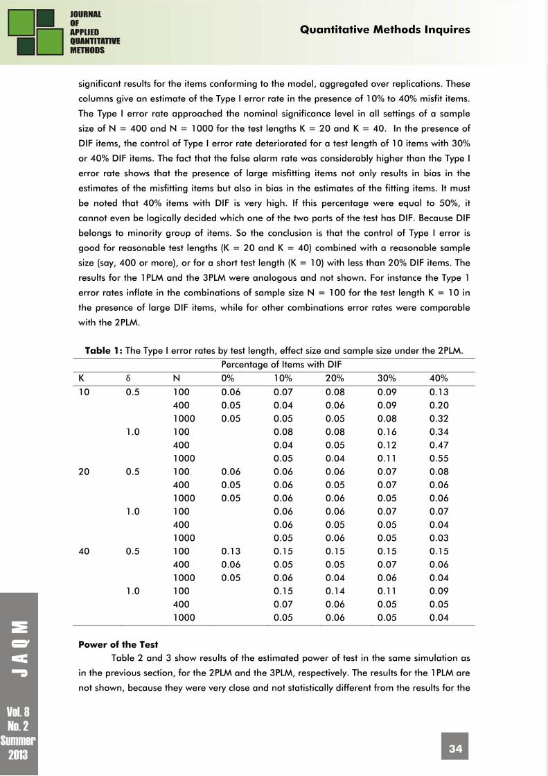
significant results for the items conforming to the model, aggregated over replications. These

columns give an estimate of the Type I error rate in the presence of 10% to 40% misfit items.

The Type I error rate approached the nominal significance level in all settings of a sample

size of N = 400 and N = 1000 for the test lengths K = 20 and K = 40. In the presence of

DIF items, the control of Type I error rate deteriorated for a test length of 10 items with 30%

or 40% DIF items. The fact that the false alarm rate was considerably higher than the Type I

error rate shows that the presence of large misfitting items not only results in bias in the

estimates of the misfitting items but also in bias in the estimates of the fitting items. It must

be noted that 40% items with DIF is very high. If this percentage were equal to 50%, it

cannot even be logically decided which one of the two parts of the test has DIF. Because DIF

belongs to minority group of items. So the conclusion is that the control of Type I error is

good for reasonable test lengths (K = 20 and K = 40) combined with a reasonable sample

size (say, 400 or more), or for a short test length (K = 10) with less than 20% DIF items. The

results for the 1PLM and the 3PLM were analogous and not shown. For instance the Type 1

error rates inflate in the combinations of sample size N = 100 for the test length K = 10 in

the presence of large DIF items, while for other combinations error rates were comparable

with the 2PLM.

Table 1: The Type I error rates by test length, effect size and sample size under the 2PLM.

Percentage of Items with DIF K δ N 0% 10% 20% 30% 40%

10 0.5 100 0.06 0.07 0.08 0.09 0.13 400 0.05 0.04 0.06 0.09 0.20 1000 0.05 0.05 0.05 0.08 0.32 1.0 100 0.08 0.08 0.16 0.34 400 0.04 0.05 0.12 0.47 1000 0.05 0.04 0.11 0.55 20 0.5 100 0.06 0.06 0.06 0.07 0.08 400 0.05 0.06 0.05 0.07 0.06 1000 0.05 0.06 0.06 0.05 0.06 1.0 100 0.06 0.06 0.07 0.07 400 0.06 0.05 0.05 0.04 1000 0.05 0.06 0.05 0.03 40 0.5 100 0.13 0.15 0.15 0.15 0.15 400 0.06 0.05 0.05 0.07 0.06 1000 0.05 0.06 0.04 0.06 0.04 1.0 100 0.15 0.14 0.11 0.09 400 0.07 0.06 0.05 0.05 1000 0.05 0.06 0.05 0.04 Power of the Test

Table 2 and 3 show results of the estimated power of test in the same simulation as

in the previous section, for the 2PLM and the 3PLM, respectively. The results for the 1PLM are

not shown, because they were very close and not statistically different from the results for the


35

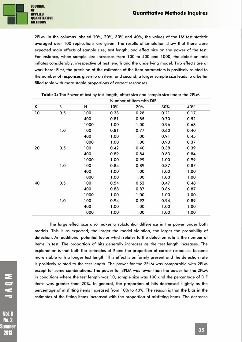
2PLM. In the columns labeled 10%, 20%, 30% and 40%, the values of the LM test statistic

averaged over 100 replications are given. The results of simulation show that there were

expected main effects of sample size, test length, and effect size on the power of the test.

For instance, when sample size increases from 100 to 400 and 1000, the detection rate

inflates considerably, irrespective of test length and the underlying model. Two effects are at

work here: First, the precision of the estimates of the item parameters is positively related to

the number of responses given to an item; and second, a larger sample size leads to a better

filled table with more stable proportions of correct responses.

The large effect size also makes a substantial difference in the power under both

models. This is as expected; the larger the model violation, the larger the probability of

detection. An additional potential factor which relates to the detection rate is the number of

items in test. The proportion of hits generally increases as the test length increases. The

explanation is that both the estimates of θ and the proportion of correct responses become

more stable with a longer test length. This effect is uniformly present and the detection rate

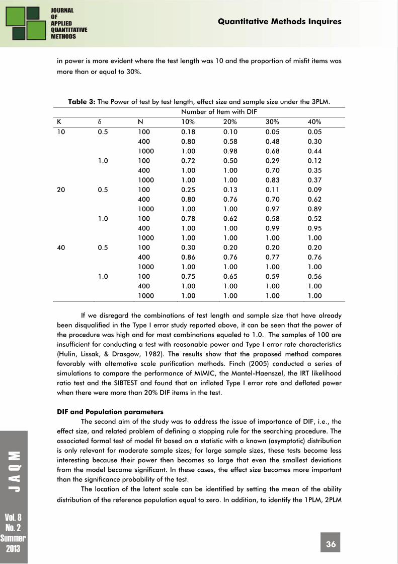
is positively related to the test length. The power for the 3PLM was comparable with 2PLM

except for some combinations. The power for 3PLM was lower than the power for the 2PLM

in conditions where the test length was 10, sample size was 100 and the percentage of DIF

items was greater than 20%. In general, the proportion of hits decreased slightly as the

percentage of misfitting items increased from 10% to 40%. The reason is that the bias in the

estimates of the fitting items increased with the proportion of misfitting items. The decrease

Table 2: The Power of test by test length, effect size and sample size under the 2PLM. Number of Item with DIF K δ N 10% 20% 30% 40%

10 0.5 100 0.33 0.28 0.21 0.17 400 0.81 0.85 0.70 0.52 1000 1.00 1.00 0.96 0.63 1.0 100 0.81 0.77 0.60 0.40 400 1.00 1.00 0.91 0.45 1000 1.00 1.00 0.93 0.37 20 0.5 100 0.42 0.40 0.38 0.39 400 0.89 0.84 0.83 0.84 1000 1.00 0.99 1.00 0.99 1.0 100 0.84 0.89 0.87 0.87 400 1.00 1.00 1.00 1.00 1000 1.00 1.00 1.00 1.00 40 0.5 100 0.54 0.52 0.47 0.48 400 0.88 0.87 0.86 0.87 1000 1.00 1.00 1.00 1.00 1.0 100 0.94 0.92 0.94 0.89 400 1.00 1.00 1.00 1.00 1000 1.00 1.00 1.00 1.00


36

in power is more evident where the test length was 10 and the proportion of misfit items was

more than or equal to 30%.

Table 3: The Power of test by test length, effect size and sample size under the 3PLM.

Number of Item with DIF K δ N 10% 20% 30% 40%

10 0.5 100 0.18 0.10 0.05 0.05 400 0.80 0.58 0.48 0.30 1000 1.00 0.98 0.68 0.44 1.0 100 0.72 0.50 0.29 0.12 400 1.00 1.00 0.70 0.35 1000 1.00 1.00 0.83 0.37 20 0.5 100 0.25 0.13 0.11 0.09 400 0.80 0.76 0.70 0.62 1000 1.00 1.00 0.97 0.89 1.0 100 0.78 0.62 0.58 0.52 400 1.00 1.00 0.99 0.95 1000 1.00 1.00 1.00 1.00 40 0.5 100 0.30 0.20 0.20 0.20 400 0.86 0.76 0.77 0.76 1000 1.00 1.00 1.00 1.00 1.0 100 0.75 0.65 0.59 0.56 400 1.00 1.00 1.00 1.00 1000 1.00 1.00 1.00 1.00

If we disregard the combinations of test length and sample size that have already been disqualified in the Type I error study reported above, it can be seen that the power of the procedure was high and for most combinations equaled to 1.0. The samples of 100 are insufficient for conducting a test with reasonable power and Type I error rate characteristics (Hulin, Lissak, & Drasgow, 1982). The results show that the proposed method compares favorably with alternative scale purification methods. Finch (2005) conducted a series of simulations to compare the performance of MIMIC, the Mantel-Haenszel, the IRT likelihood ratio test and the SIBTEST and found that an inflated Type I error rate and deflated power when there were more than 20% DIF items in the test. DIF and Population parameters

The second aim of the study was to address the issue of importance of DIF, i.e., the effect size, and related problem of defining a stopping rule for the searching procedure. The associated formal test of model fit based on a statistic with a known (asymptotic) distribution is only relevant for moderate sample sizes; for large sample sizes, these tests become less interesting because their power then becomes so large that even the smallest deviations from the model become significant. In these cases, the effect size becomes more important than the significance probability of the test.

The location of the latent scale can be identified by setting the mean of the ability

distribution of the reference population equal to zero. In addition, to identify the 1PLM, 2PLM


37

and 3PLM, the variance of the reference population can be set to 1.0. In the stepwise

procedure defined above an identified DIF item is given group specific item parameters and

new MML estimates of the item parameters and the parameters of the ability distribution are

made. In the present case, the relevant ability distribution parameters are those of the focal

population. It is assumed that the change in the estimates between steps gives an indication

of the importance of the identified DIF.

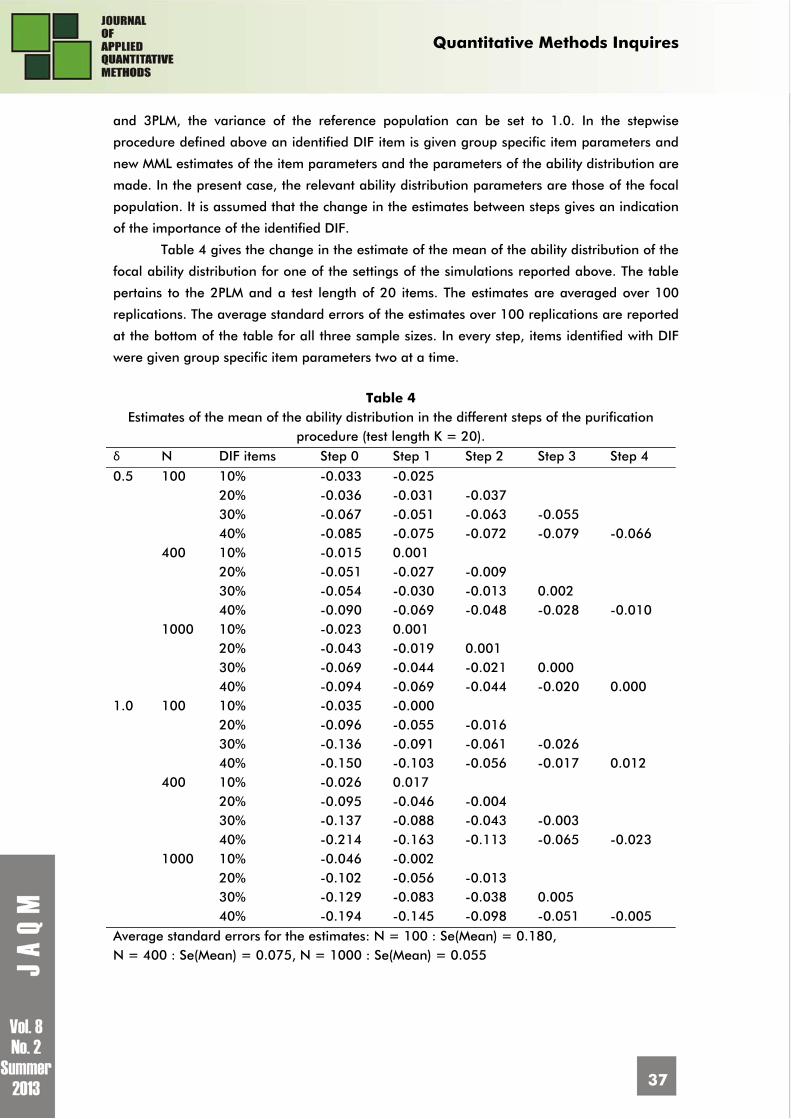
Table 4 gives the change in the estimate of the mean of the ability distribution of the

focal ability distribution for one of the settings of the simulations reported above. The table

pertains to the 2PLM and a test length of 20 items. The estimates are averaged over 100

replications. The average standard errors of the estimates over 100 replications are reported

at the bottom of the table for all three sample sizes. In every step, items identified with DIF

were given group specific item parameters two at a time.

Table 4

Estimates of the mean of the ability distribution in the different steps of the purification procedure (test length K = 20).

δ N DIF items Step 0 Step 1 Step 2 Step 3 Step 4

0.5 100 10% -0.033 -0.025 20% -0.036 -0.031 -0.037 30% -0.067 -0.051 -0.063 -0.055 40% -0.085 -0.075 -0.072 -0.079 -0.066 400 10% -0.015 0.001 20% -0.051 -0.027 -0.009 30% -0.054 -0.030 -0.013 0.002 40% -0.090 -0.069 -0.048 -0.028 -0.010 1000 10% -0.023 0.001 20% -0.043 -0.019 0.001 30% -0.069 -0.044 -0.021 0.000 40% -0.094 -0.069 -0.044 -0.020 0.000 1.0 100 10% -0.035 -0.000 20% -0.096 -0.055 -0.016 30% -0.136 -0.091 -0.061 -0.026 40% -0.150 -0.103 -0.056 -0.017 0.012 400 10% -0.026 0.017 20% -0.095 -0.046 -0.004 30% -0.137 -0.088 -0.043 -0.003 40% -0.214 -0.163 -0.113 -0.065 -0.023 1000 10% -0.046 -0.002 20% -0.102 -0.056 -0.013 30% -0.129 -0.083 -0.038 0.005 40% -0.194 -0.145 -0.098 -0.051 -0.005 Average standard errors for the estimates: N = 100 : Se(Mean) = 0.180, N = 400 : Se(Mean) = 0.075, N = 1000 : Se(Mean) = 0.055


38

The column labeled ‘Step 0’ gives the estimates of the means in the initial MML

analysis, where no items were treated yet. The true means were all equal to zero, so it can

be seen that there was a clear main-effect of the percentage of DIF items present. To some

extent, sample size has an effect on the precision of estimates which can be seen at the

bottom of the table. Further, it can be seen that in the final step of the procedure the

estimates approach the true value of zero. In practice, the true value is of course not known

and therefore the convergence of the procedure must be judged from the differences in the

estimates between steps. In the present example, only uniform DIF was generated and as a

consequence, there was no systematic trend in the estimates of the variances of the ability

distributions. All estimates were sufficiently close to the true value of 1.0. As will become

clear in the next section, this no longer holds when non-uniform DIF is present.

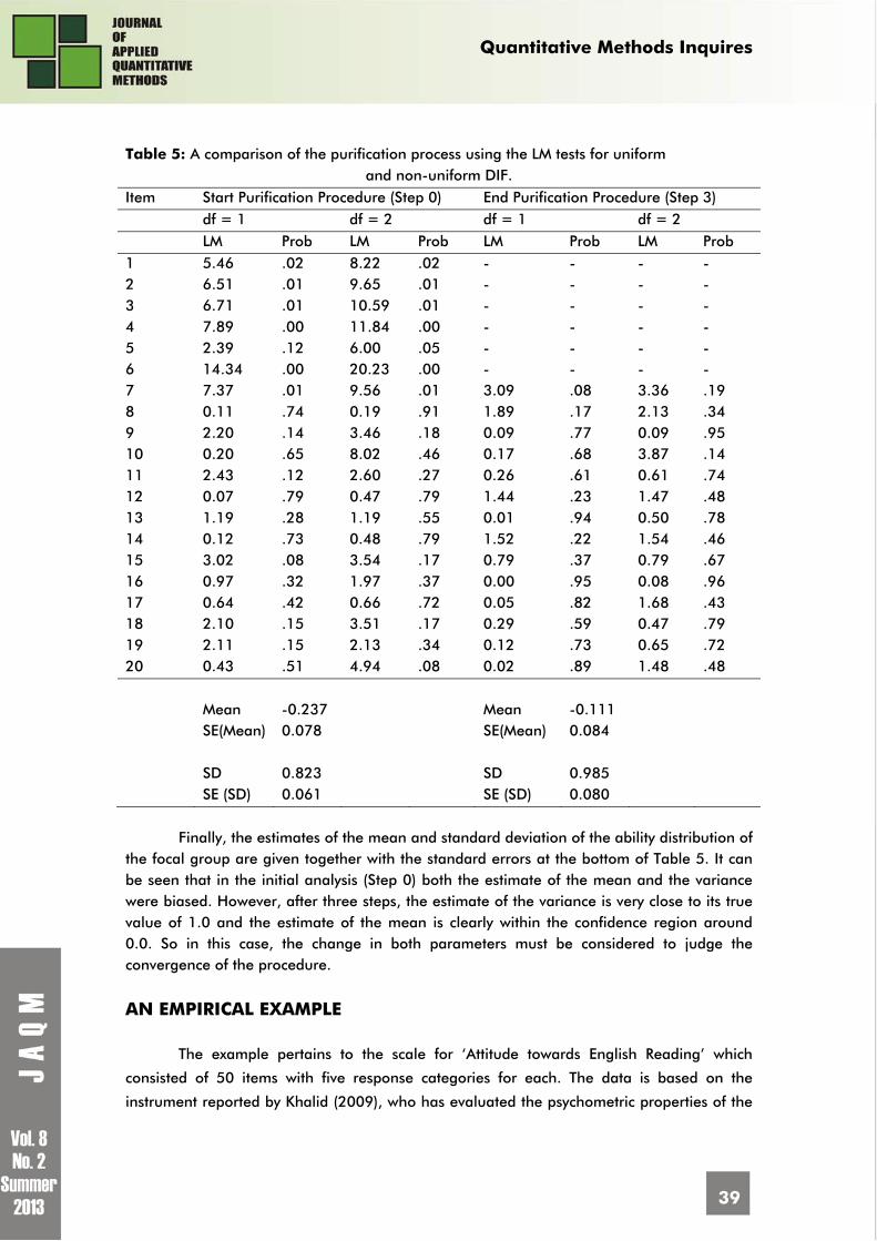
Non-uniform DIF

In the previous sections, the focus was on uniform DIF. In this part, a simulated

example of non-uniform DIF is presented. In non-uniform DIF, usually both the difficulty and

discrimination parameters differ between groups. Using the same setup as in the previous

simulations, a dataset of 20 items was simulated using the 2PLM. DIF was imposed on the

first 6 items of the test by choosing 0.50i and 0.50i . So in the focal group the

discrimination parameters of the DIF items were lowered from 1.0 to 0.5 and the item

difficulties rose from 0.0 to 0.5. This might reflect the situation where the respondents of the

focal group were less motivated to make an effort on these items, which resulted in a lower

probability of a correct response and an attenuated relation between the responses and the

latent ability dimension. One of the questions of interest was the relation between the test

targeted at uniform DIF (null-hypothesis 0i ) and test targeted at non-uniform DIF (null-

hypothesis 0i and 0i ). The results are shown in Table 6. The columns 3 to 5 pertain

to the first MML analysis where none of the items were given group-specific item parameters

yet, the columns 6 to 9 pertain to the situation after the third step when 6 items where

identified as DIF items. Note that all 6 items were correctly identified. The columns under the

label ‘df = 1’ concern the test for 0i , which has one degree of freedom; the columns

under the label ‘df = 2’ refer to the test for 0i and 0i , which has two degrees of

freedom. Note that the test with one degree of freedom seems to have a higher power: in

19 cases its significance probability is lower than the significance probability of the test with

two degrees of freedom. The latter test has the lowest significance probability in 8 cases. So

in practice, the test with two-degrees of freedom will not add much information over the test

with one degree of freedom. One may notice that Item 7 was significant before the start of

purification procedure (Step 0) under 1-df and 2-df test but it becomes non-significant at the

end of the purification procedure (Step 3).


39

Table 5: A comparison of the purification process using the LM tests for uniform

and non-uniform DIF. Item Start Purification Procedure (Step 0) End Purification Procedure (Step 3) df = 1 df = 2 df = 1 df = 2 LM Prob LM Prob LM Prob LM Prob 1 5.46 .02 8.22 .02 - - - - 2 6.51 .01 9.65 .01 - - - - 3 6.71 .01 10.59 .01 - - - - 4 7.89 .00 11.84 .00 - - - - 5 2.39 .12 6.00 .05 - - - - 6 14.34 .00 20.23 .00 - - - - 7 7.37 .01 9.56 .01 3.09 .08 3.36 .19 8 0.11 .74 0.19 .91 1.89 .17 2.13 .34 9 2.20 .14 3.46 .18 0.09 .77 0.09 .95 10 0.20 .65 8.02 .46 0.17 .68 3.87 .14 11 2.43 .12 2.60 .27 0.26 .61 0.61 .74 12 0.07 .79 0.47 .79 1.44 .23 1.47 .48 13 1.19 .28 1.19 .55 0.01 .94 0.50 .78 14 0.12 .73 0.48 .79 1.52 .22 1.54 .46 15 3.02 .08 3.54 .17 0.79 .37 0.79 .67 16 0.97 .32 1.97 .37 0.00 .95 0.08 .96 17 0.64 .42 0.66 .72 0.05 .82 1.68 .43 18 2.10 .15 3.51 .17 0.29 .59 0.47 .79 19 2.11 .15 2.13 .34 0.12 .73 0.65 .72 20 0.43 .51 4.94 .08 0.02 .89 1.48 .48 Mean -0.237 Mean -0.111 SE(Mean) 0.078 SE(Mean) 0.084 SD 0.823 SD 0.985 SE (SD) 0.061 SE (SD) 0.080

Finally, the estimates of the mean and standard deviation of the ability distribution of the focal group are given together with the standard errors at the bottom of Table 5. It can be seen that in the initial analysis (Step 0) both the estimate of the mean and the variance were biased. However, after three steps, the estimate of the variance is very close to its true value of 1.0 and the estimate of the mean is clearly within the confidence region around 0.0. So in this case, the change in both parameters must be considered to judge the convergence of the procedure.

AN EMPIRICAL EXAMPLE

The example pertains to the scale for ‘Attitude towards English Reading’ which

consisted of 50 items with five response categories for each. The data is based on the

instrument reported by Khalid (2009), who has evaluated the psychometric properties of the


40

scale and found it to be appropriate for similar studies. The scale was administered to 8th

grade students in a number of elementary schools in Pakistan. The respondents were divided

into two groups on the basis of gender. The sample consisted of 1080 boys and 1553 girls.

The item parameters were estimated by MML assuming standard normal distributions for the

θ-parameters of both groups.

Table 6 gives the results for the LM test of the hypothesis 0i . The table only

shows the first 14 items plus the 6 items with the most significant results in the remaining 36

items. We have not presented rest of items due to space limitation. The column labeled ‘LM’

gives the values of the LM-statistics and the column labeled ‘Prob’ shows the significance of

the probabilities. The statistics have one degree of freedom. Ten of the fifty LM-tests were

significant at a 5% significance level. The observed item-total scores (first term in equation

11) and expected item-total scores (second term in equation 11) averaged over the two

groups are shown under the headings ‘Obs’ and ‘Exp’, respectively. To get an impression of

the effect size of the misfit, the mean absolute difference between the observed and

expected item-total scores are given under the heading “Abs.Diff”. The observed and

expected values were quite close: the mean absolute difference was approximately .02 and

the largest absolute difference was .19. This analysis was the starting point for the iterative

procedure of identification and modeling of DIF. The item with the largest LM value, Item 37,

was split into two virtual items, one that was supposed to be given to the boys and one that

was supposed to be given to the girls. New MML estimates were made and the next item

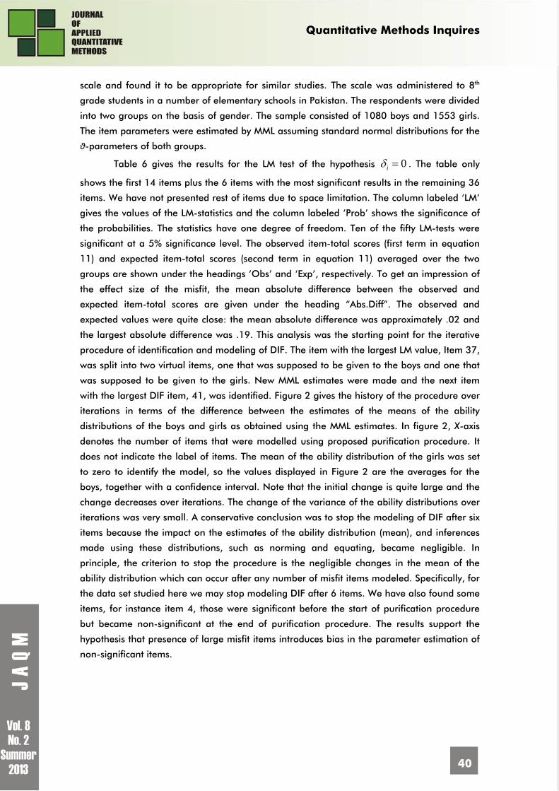
with the largest DIF item, 41, was identified. Figure 2 gives the history of the procedure over

iterations in terms of the difference between the estimates of the means of the ability

distributions of the boys and girls as obtained using the MML estimates. In figure 2, X-axis

denotes the number of items that were modelled using proposed purification procedure. It

does not indicate the label of items. The mean of the ability distribution of the girls was set

to zero to identify the model, so the values displayed in Figure 2 are the averages for the

boys, together with a confidence interval. Note that the initial change is quite large and the

change decreases over iterations. The change of the variance of the ability distributions over

iterations was very small. A conservative conclusion was to stop the modeling of DIF after six

items because the impact on the estimates of the ability distribution (mean), and inferences

made using these distributions, such as norming and equating, became negligible. In

principle, the criterion to stop the procedure is the negligible changes in the mean of the

ability distribution which can occur after any number of misfit items modeled. Specifically, for

the data set studied here we may stop modeling DIF after 6 items. We have also found some

items, for instance item 4, those were significant before the start of purification procedure

but became non-significant at the end of purification procedure. The results support the

hypothesis that presence of large misfit items introduces bias in the parameter estimation of

non-significant items.


41

0

0.05

0.1

0.15

0.2

0.25

0.3

0.35

0.4

0.45

0.5

0 1 2 3 4 5 6 7 8 9 10

Numbers of DIF items identified and modeled

Ch

ang

e Mean

Mean + SE

Mean - SE

Figure2: Change in the estimates of the means of the ability distribution over iterations.

Table 6 The results of LM test to evaluate fit of DIF.

Boys Girls

Item LM Prob Obs Exp Obs Exp Abs.Diff

1 1.09 0.30 2.75 2.70 2.49 2.52 0.04 2 0.95 0.33 3.28 3.25 3.05 3.07 0.03 3 2.70 0.10 3.23 3.18 2.94 2.98 0.04 4 6.20 0.01 3.26 3.19 2.91 2.96 0.06 5 2.45 0.12 2.70 2.76 2.65 2.60 0.05 6 3.40 0.07 3.27 3.21 2.97 3.01 0.05 7 1.02 0.31 3.13 3.16 2.97 2.95 0.02 8 2.88 0.09 2.93 2.98 2.76 2.72 0.05 9 0.40 0.53 3.11 3.13 2.91 2.89 0.02 10 0.03 0.86 2.99 2.98 2.79 2.79 0.01 11 0.20 0.65 2.67 2.65 2.44 2.46 0.02 12 0.68 0.41 3.05 3.08 2.91 2.90 0.02 13 3.28 0.07 3.32 3.27 3.00 3.03 0.04 14 2.81 0.09 2.78 2.84 2.71 2.67 0.05 25 8.50 0.00 3.02 3.11 2.95 2.88 0.08 30 8.26 0.00 3.32 3.23 2.96 3.02 0.07 33 4.51 0.03 3.14 3.08 2.81 2.85 0.06 37 20.18 0.00 1.87 2.09 2.01 1.86 0.19 41 14.21 0.00 2.30 2.48 2.41 2.28 0.15 50 5.13 0.02 3.44 3.38 3.15 3.20 0.06


42

DISCUSSION AND CONCLUSION

IRT is widely used in the field of educational and psychological testing for evaluation of the reliability and validity of tests, optimal item selection, computerized adaptive testing, developing and refining exams, maintaining item banks and equating the difficulty of successive versions of examinations. However, these applications assume that the IRT model used hold. The presence of misfitting items may potentially threaten the realization of the advantages of IRT models. The topic of model-fit has, over the course of the past few decades, become of increasing interest to test developers and measurement practitioners. It is widely known that DIF is one of the most important threats to IRT model fit. A method for the analysis of DIF has been proposed in this paper that addresses two issues. The first issue is that the presence of a large number of items with DIF has an impact on the detection of statistical search procedures for DIF. Several scale purification procedures have been developed to address this threat to DIF contamination, as we have argued, if test have many DIF items, then DIF contamination cannot be eliminated completely by scale purification procedures. A stepwise purification procedure has been proposed in this paper that consisted of alternating between identifying DIF using an LM test and modeling DIF using group-specific item parameters. The second issue is the importance of DIF and the related issue of when to stop searching for DIF and modeling DIF. Many applications of IRT entail inferences about the latent ability distribution. Such as of norming and standard setting, linking and equating, the estimation of group differences and linear regression models on ability parameters as used in large scale education surveys. We highlighted the importance of DIF and its relationship to ability distributions and demonstrated that in order to monitor the purification procedure, we need to use the change of the estimates of the parameters of the ability distributions over the steps of the procedure.

We provided evidence from simulation studies to assess the Type I error rate and power of the procedure. It was concluded that our proposed procedure worked well for sample sizes from 400 respondents and test lengths from 20 items. For a test length of ten items, the procedure only worked well when the proportion of DIF items was 10% and 20%. In all situations, the power slightly decreased with the increasing number of DIF items. The power for the 3PLM was less than the power for the 2PLM specifically in settings of test length K = 10 and percentage of DIF items greater than 20%. The proposed stepwise procedure performs quite well in terms of power and Type1 error rates. The performance of stepwise LM test was optimal over well documented statistical methods in the presence of 20% or more DIF item which are reported in Finch (2005). In the case of uniform DIF, it was shown that DIF biased the estimates of the means of the ability distributions, but this bias vanished in the course of the stepwise purification procedure when DIF was modeled by the introduction of group-specific item parameters. In the case of non-uniform DIF, both the mean and variance of the ability distributions were biased, we have shown that this bias could be removed with group-specific item parameters. Finally, the simulation studies illustrated that the LM test targeted at uniform DIF was sufficiently sensitive to a combination of uniform and non-uniform DIF and the inferences did not change when the LM test for non-uniform DIF was used.

One of the advantages of using LM tests for evaluation of item fit is that the asymptotic distribution of the statistics involved follows directly from asymptotic theory.


43

Therefore, the approach can easily be generalized to other model violations and other IRT models. Examples are the application of the approach to IRT models for polytomous items, evaluation of local independence, shape of item response function, assessment of dimensionality, test speededness and evaluation of person fit.

REFERENCES 1. Aitchison, J., & Silvey, S. D., Maximum likelihood estimation of parameters subject

to restraints. Annals of Mathematical Statistics, 29, 1958, 813-828.

2. Andersen, E.B, Discrete statistical models with social science applications. Amsterdam, North Holland, 1980.

3. Béguin, A. A., & Glas, C. A. W., MCMC estimation and some model-fit analysis of multidimensional IRT models. Psychometrika, 66, 2001, 541-561.

4. Birnbaum, A., Some latent trait models and their use in inferring an examinees ability. In F. M. Lord & M. R. Novick (Eds.), Statistical theories of mental test scores, 1968, (pp. 397-424). Reading MA: Addison-Wesley.

5. Bock, R. D. Estimating item parameters and latent ability when responses are scored in two or more nominal categories. Psychometrika, 37, 1972, 29-51.

6. Bock, R. D., & Aitkin, M., Marginal maximum likelihood estimation of item parameters: Application of an EM algorithm. Psychometrika, 46, 1981, 443–459.

7. Bock, R. D., & Zimowski, M. F., Multiple Group IRT. In W. J. van der Linden & R. K. Hambleton (Eds.), Handbook of Modern Item Response Theory. New York: Springer Verlag, 1997, 433-448.

8. Candell, G. L., & Drasgow, F., An iterative procedure for linking metrics and assessing item bias in item response theory. Applied Psychological Measurement, 12, 1988, 253-260.

9. Camilli, G. A conceptual analysis of differential item functioning in terms of a multidimensional item response model. Applied Psychological Measurement, 16, 1992, 129-147.

10. Camilli, G., & Shepard, L. A., Methods for identifying biased test items. Thousand Oaks, CA: Sage, 1994.

11. Clauser, B. E., Mazor, K. M., & Hambleton, R. K., The effects of purification of the matching criterion on the identification of DIF using the Mantel-Haenszel procedure. Applied Measurement in Education, 6, 1993, 269-279.

12. Clauser, B. E., & Mazor, K. M., Using statistical procedures to identify differential item functioning test items. Educational Measurement: Issues and Practice, 17, 1998, 31-44.


44

13. Dorans, N.J., & Kulick, E., Demonstrating the utility of the standardization approach to assessing unexpected differential item performance on the Scholastic Aptitude Test. Journal of Educational Measurement, 23, 1968, 355-368.

14. Efron, B., Discussion on maximum likelihood from incomplete data via the EM algorithm (by A. Dempster, N. Liard, and D. Rubin). Journal of the Royal Statistical Society, Series B, 39, 1977, 1-38.

15. Embretson, S.E., & Reise, S.P. Item Response Theory for Psychologists. Hillsdale, NJ: Lawrence Erlbaum Associates, 2000

16. Finch, H., The MIMIC model as a method for detecting DIF: Comparison with Mantel-Haenszel, SIBTEST, and the IRT likelihood ratio. Applied Psychological Measurement, 29, 2005, 278-295.

17. Fischer, G.H., Notes on the Mantel-Haenszel procedure and another chi-squared test for the assessment of DIF. Methodika, 7, 1993, 88-100.

18. Fischer, G.H., Some neglected problems in IRT. Psychometrika, 60, 1995, 449-487.

19. Fox, J.P., & Glas, C.A.W., Bayesian modification indices for IRT models. Statistica Neerlandica, 59, 2005, 95-106.

20. French, B. F., & Maller, S. J., Iterative purification and effect size use with logistic regression for differential item functioning detection. Educational and Psychological Measurement, 67, 2007, 373-393.

21. Glas, C. A. W. Detection of differential item functioning using Lagrange multiplier tests. Statistica Sinica, 8, 1998, 647-667.

22. Glas, C. A. W., Modification indices for the 2PLM and the nominal response model. Psychometrika, 64, 1999, 273-294.

23. Glas, C.A.W., & Dagohoy, A.V. T., A person fit test for IRT models for polytomous items. Psychometrika, 72, 2007, 159-180.

24. Glas, C. A. W., & Falcón, J. C. S. A comparison of item-fit statistics for the three-parameter logistic model. Applied Psychological Measurement. 27, 2003, 87-106.

25. Glas, C. A. W., & Meijer, R. R., A Bayesian approach to person fit analysis in item response theory models. Applied Psychological Measurement, 27, 2003, 217-233.

26. Hidalgo-Montesinos, M.D., & Gómez-Benito, J., Test purification and the evaluation of differential item functioning with multinomial logistic regression. European Journal of Psychological Assessment, 19, 2003, 1-11.

27. Holland, P. W., & Thayer, D. T., Differential item performance and the Mantel-Haenszel procedure. In H. Holland & H. I. Braun (Eds.), Test validity (pp. 129-145). Hillsdale, NJ: Lawrence Erlbaum, 1988.


45

28. Holland, P. W., & Wainer, H., Differential item functioning. Hillsdale, NJ: Lawrence Erlbaum, 1993.

29. Hulin, C. L., Lissak, R. I., & Drasgow, R., Recovery of two- and three-parameter logistic item characteristic curves: A monte carlo study. Applied Psychological Measurement, 6, 1982, 249-260.

30. Jansen, M. G. H., & Glas, C. A. W. (2001). Statistical tests for differential test functioning in Rasch’s model for speed tests. In A. Boomsma, M. A. J. van Duijn, & T. A. B. Snijders (Eds.), Essays on item response theory, 2001, pp. 149-162, New York: Springer.

31. Jansen, M., & Glas, C. A. W., Checking the Assumptions of Rasch's Model for Speed Tests. Psychometrika, 70, 2005, 671-684.

32. Kelderman, H., & Macready, G.B., The use of loglinear models for assessing differential item functioning across manifest and latent examinee groups. Journal of Educational Measurement, 27, 1990, 307-327.

33. Kalid, M. N., IRT model fit from different perspectives. Doctoral dissertation, University of Twente, The Netherlands, 2009.

34. Khalid, M. N., A Comparison of Top-down and Bottom-up approaches in the Identification of Differential Item Functioning using Confirmatory Factor Analysis. The International Journal of Educational and Psychological Assessment, 7, 2011, 1-18.

35. Lautenschlager, G. J., Flaherty, V. L., & Park, D. G., IRT differential item functioning: An examination of ability scale purifications. Educational and Psychological Measurement, 54, 1994, 21-31.

36. Lord, F.M., Applications of item response theory to practical testing problems. Hillsdale: Lawrence Erlbaum, 1980.

37. Lord, F. M., & Novick, M. R., Statistical theories of mental test scores. Reading M.A: Addison-Wesley, 1968.

38. Louis, T.A., Finding the observed information matrix when using the EM algorithm. Journal of the Royal Statistical Society, Series B, 44, 1982, 226–233.

39. Masters, G. N., A Rasch model for partial credit scoring. Psychometrika 47, 1982, 149-174.

40. Meredith, W., & Millsap, R.E., On the misuse of manifest variables in the detection of measurement bias. Psychometrika, 57, 1992, 289–311.

41. Miller, M. D., & Oshima, T. C., Effect of sample size, number of biased items, and magnitude of bias on a two-stage item bias estimation method. Applied Psychological Measurement, 16, 1992, 381-388.


46

42. Millsap, R. E., & Everson, H. T., Methodology review: Statistical approaches for assessing measurement bias. Applied Psychological Measurement, 17, 1993, 297-334.

43. Mislevy, R. J., Estimating latent distributions. Psychometrika, 49, 1984, 359–381.

44. Mislevy, R. J., Bayes modal estimation in item response models. Psychometrika, 51, 1986, 177–195.

45. Muraki, E., A generalized partial credit model: application of an EM algorithm. Applied Psychological Measurement, 16, 1992, 159-176.

46. Muthén, B. O., Some uses of structural equation modeling in validity studies: Extending IRT to external variables. In H. Wainer & H. Braun (Eds.), Test validity (pp. 213-238). Hillsdale, NJ: Lawrence Erlbaum, 1988.

47. Navas-Ara, M. J., & Gómez-Benito, J., Effects of ability scale purification on identification of DIF. European Journal of Psychological Assessment, 18, 2002, 9-15.

48. Park, D. G., & Lautenschlager, G. J. Improving IRT item bias detection with iterative linking and ability scale purification. Applied Psychological Measurement, 14, 1990, 163-173.

49. Penfield, R.D., & Camilli, G., Differential item functioning and item bias. In S. Sinharay & C.R. Rao (Eds.), Handbook of Statistics, Volume 26: Psychometrics (pp. 125-167). New York: Elsevier, 2007.

50. Raju, N. S., The area between two item characteristic curves. Psychometrika, 53, 1988, 495-502.

51. Rao, C. R., Large sample tests of statistical hypothesis concerning several parameters with applications to problems of estimation. Proceedings of Cambridge Philosophical Society 44, 1948, 50-57.

52. Rasch, G., Probabilistic Models for Some Intelligence and Attainment Tests. Copenhagen: Danish Institute for Educational Research, 1960.

Rigdon, S. E., & Tsutakawa, R. K., Estimation in latent trait models. Psychometrika, 48, 1983, 567-574.

53. Roussos, L. A., & Stout, W. F., Simulation studies of the effects of small sample size and studied item parameters on SIBTEST and Mantel-Haenszel type I error performance. Journal of Educational Measurement, 33, 1996, 215-230.

54. Roussos, L. A., & Stout, W. F., Differential item functioning analysis. In D. Kaplan (Ed.), The Sage handbook of quantitative methodology for the social sciences (pp. 107-116). Thousand Oaks, CA: Sage, 2004.

55. Shealy, R., & Stout, W. F., A model-based standardization approach that separates true bias/DIF from group differences and detects test bias/DIF as well as item bias/DIF. Psychometrika, 58, 1993, 159-194.


47

56. Shih, C.-L., & Wang, W.-C., Differential Item Functioning Detection Using the Multiple Indicators, Multiple Causes Method with a Pure Short Anchor. Applied Psychological Measurement, 33, 2009, 184-199.

57. Silvey, S. D., The Lagrangian multiplier test. Annals of Mathematical Statistics, 30, 1959, 389-407.

58. Sörbom, D., Model modification. Psychometrika, 54, 1989, 371-384.

59. Swaminathan, H., & Rogers, H.J., Detecting differential item functioning using logistic regression procedures. Journal of Educational Measurement, 27, 1990, 361-370.

60. Thissen, D., Steinberg, L., & Wainer, H., Use of item response theory in the study of group differences in trace lines. In H. Wainer & H. I. Braun (Eds.), Test validity (pp. 147-169). Hillsdale, NJ: Lawrence Erlbaum, 1988.

61. Thissen, D., Steinberg, L., & Wainer, H., Detection of differential item functioning using the parameters of item response models. In P.W. Holland & H. Wainer (Eds.), Differential item functioning. Hillsdale, NJ: Lawrence Erlbaum Associates, 67-113, 1993.

62. Wang, W.-C., & Su, Y.-H., Effects of average signed area between two item characteristic curves and test purification procedures on the DIF detection via the Mantel-Haenszel method. Applied Measurement in Education, 17, 2004, 113-144.

63. Wang,W.-C., & Su, Y.-H., Factors Influencing the Mantel and generalized Mantel-Haenszel methods for the assessment of differential item functioning in polytomous items. Applied Psychological Measurement, 28, 2004, 450-480.

64. Wang,W.-C., & Su, Y.-H., MIMIC Methods for Assessing Differential Item Functioning in Polytomous Items. Applied Psychological Measurement, 34, 2010, 166-180.

65. Zimowski, M.F., Muraki, E., Mislevy, R.J., & Bock, R.D., Bilog MG: Multiple-group IRT analysis and test maintenance for binary items. Chicago: Scientific Software International, Inc., 1996

Documents

A STEP-WISE METHOD FOR EVALUATION OF DIFFERENTIAL ITEM FUNCTIONING …issue-2/pdfs/3_khalid.pdf · A STEP-WISE METHOD FOR EVALUATION OF DIFFERENTIAL ITEM FUNCTIONING Muhammad Naveed