Analysis of Clocked Sequential Circuits Objectives The objectives of this lesson are as follows:

Analysis of clocked sequential circuits with an example

State Reduction with an example

State assignment

Design with unused states

Unused state hazards

Figure 1: Sequential Circuit Design Steps

The behavior of a sequential circuit is determined from the inputs, outputs and states of its flip-flops. Both the outputs and the next state are a function of the inputs and the present state. Recall from previous lesson that sequential circuit design involves the flow as shown.

1

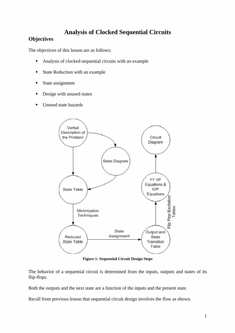
Analysis consists of obtaining a state-table or a state-diagram from a given sequential circuit implementation. In other words analysis closes the loop by forming state-table from a given circuit-implementation. We will show the analysis procedure by deriving the state table of the example circuit we considered in synthesis. The circuit is shown in Figure.

Figure 2: A Clocked sequential circuit

The circuit has

Clock input, CP. One input x One output y One clocked JK flip-flop One clocked D flip-flop (the machine can be in maximum of 4 states)

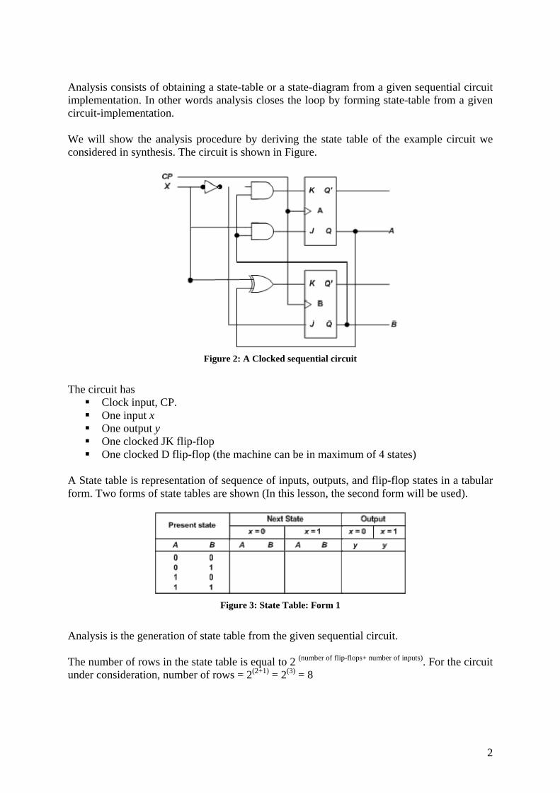
A State table is representation of sequence of inputs, outputs, and flip-flop states in a tabular form. Two forms of state tables are shown (In this lesson, the second form will be used).

Figure 3: State Table: Form 1

Analysis is the generation of state table from the given sequential circuit. The number of rows in the state table is equal to 2 (number of flip-flops+ number of inputs). For the circuit under consideration, number of rows = 2(2+1) = 2(3) = 8

2

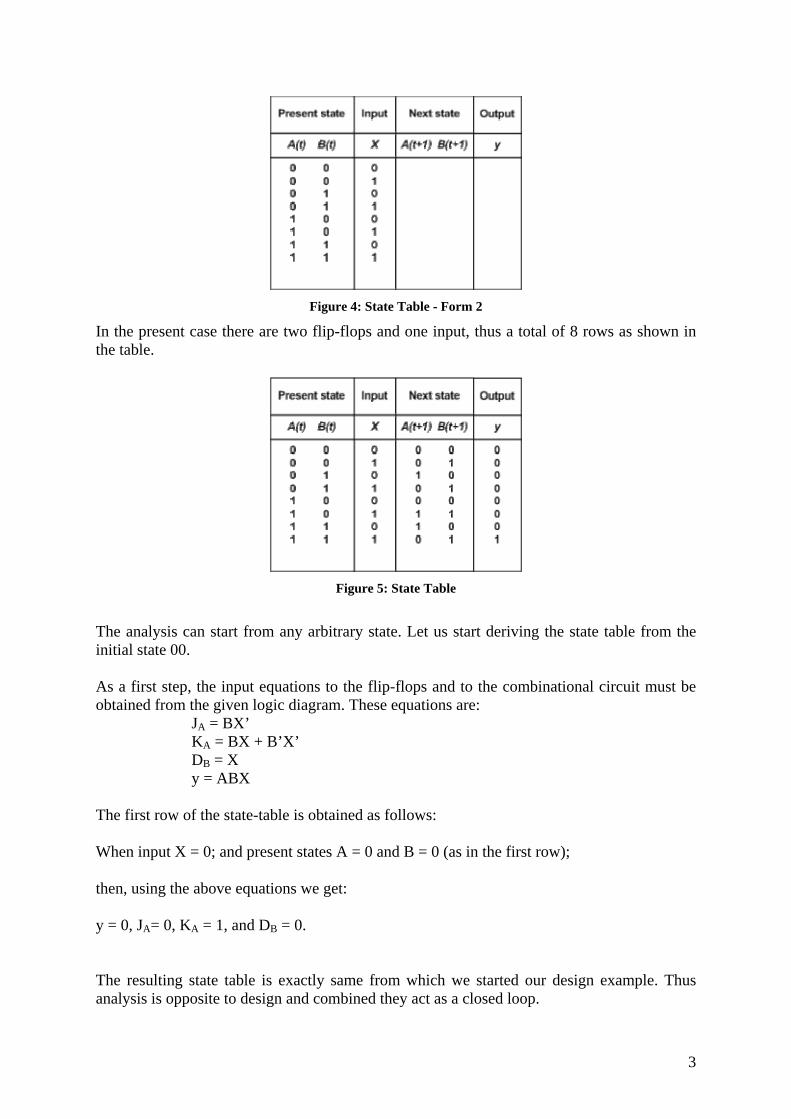
Figure 4: State Table - Form 2

In the present case there are two flip-flops and one input, thus a total of 8 rows as shown in the table.

Figure 5: State Table

The analysis can start from any arbitrary state. Let us start deriving the state table from the initial state 00. As a first step, the input equations to the flip-flops and to the combinational circuit must be obtained from the given logic diagram. These equations are:

JA = BX’ KA = BX + B’X’ DB = X y = ABX

The first row of the state-table is obtained as follows: When input X = 0; and present states A = 0 and B = 0 (as in the first row); then, using the above equations we get: y = 0, JA= 0, KA = 1, and DB = 0. The resulting state table is exactly same from which we started our design example. Thus analysis is opposite to design and combined they act as a closed loop.

3

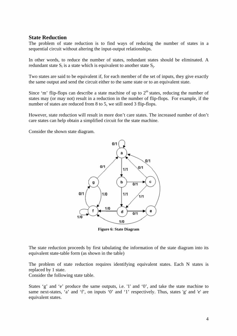
State Reduction The problem of state reduction is to find ways of reducing the number of states in a sequential circuit without altering the input-output relationships. In other words, to reduce the number of states, redundant states should be eliminated. A redundant state Si is a state which is equivalent to another state Sj. Two states are said to be equivalent if, for each member of the set of inputs, they give exactly the same output and send the circuit either to the same state or to an equivalent state. Since ‘m’ flip-flops can describe a state machine of up to 2m states, reducing the number of states may (or may not) result in a reduction in the number of flip-flops. For example, if the number of states are reduced from 8 to 5, we still need 3 flip-flops. However, state reduction will result in more don’t care states. The increased number of don’t care states can help obtain a simplified circuit for the state machine. Consider the shown state diagram.

Figure 6: State Diagram

The state reduction proceeds by first tabulating the information of the state diagram into its equivalent state-table form (as shown in the table) The problem of state reduction requires identifying equivalent states. Each N states is replaced by 1 state. Consider the following state table. States ‘g’ and ‘e’ produce the same outputs, i.e. '1' and ‘0’, and take the state machine to same next-states, ‘a’ and ‘f’, on inputs ‘0’ and ‘1’ respectively. Thus, states 'g' and 'e' are equivalent states.

4

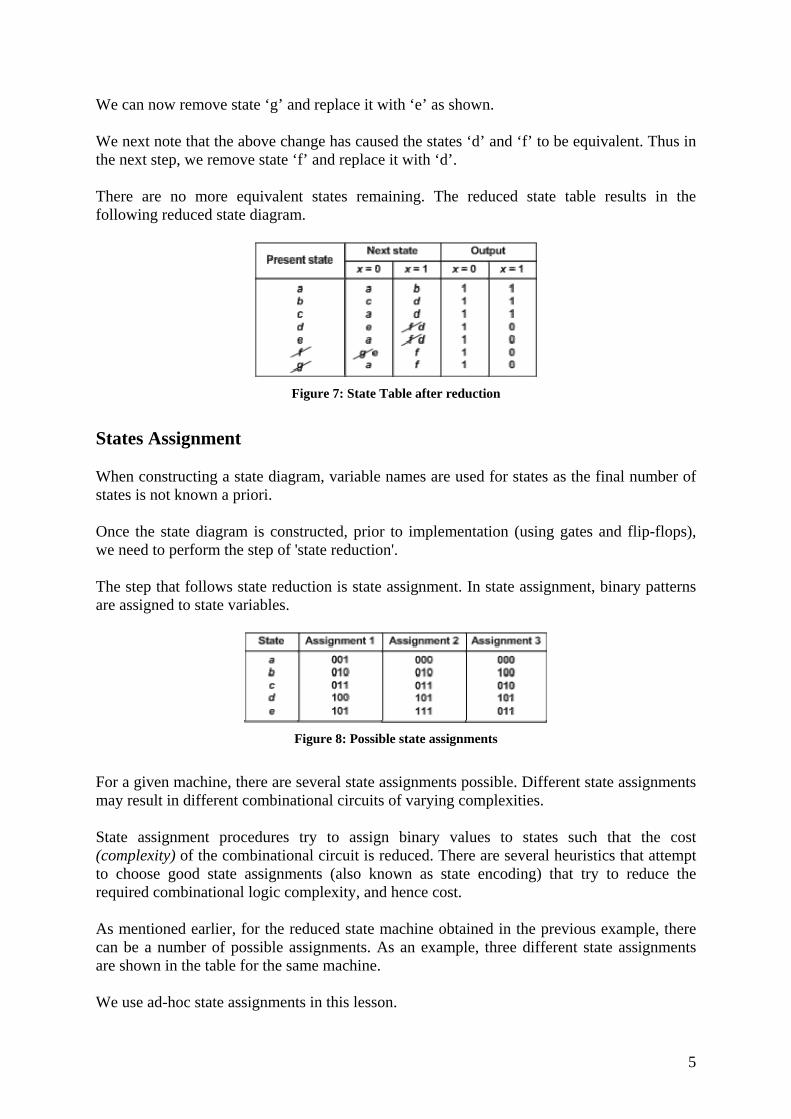
We can now remove state ‘g’ and replace it with ‘e’ as shown. We next note that the above change has caused the states ‘d’ and ‘f’ to be equivalent. Thus in the next step, we remove state ‘f’ and replace it with ‘d’. There are no more equivalent states remaining. The reduced state table results in the following reduced state diagram.

Figure 7: State Table after reduction

States Assignment When constructing a state diagram, variable names are used for states as the final number of states is not known a priori. Once the state diagram is constructed, prior to implementation (using gates and flip-flops), we need to perform the step of 'state reduction'. The step that follows state reduction is state assignment. In state assignment, binary patterns are assigned to state variables.

Figure 8: Possible state assignments

For a given machine, there are several state assignments possible. Different state assignments may result in different combinational circuits of varying complexities. State assignment procedures try to assign binary values to states such that the cost (complexity) of the combinational circuit is reduced. There are several heuristics that attempt to choose good state assignments (also known as state encoding) that try to reduce the required combinational logic complexity, and hence cost. As mentioned earlier, for the reduced state machine obtained in the previous example, there can be a number of possible assignments. As an example, three different state assignments are shown in the table for the same machine. We use ad-hoc state assignments in this lesson.

5

Design with unused states There are occasions when a sequential circuit, implemented using m flip-flops, may not utilize all the possible 2m states

Figure 9: Reduced table with binary assignments

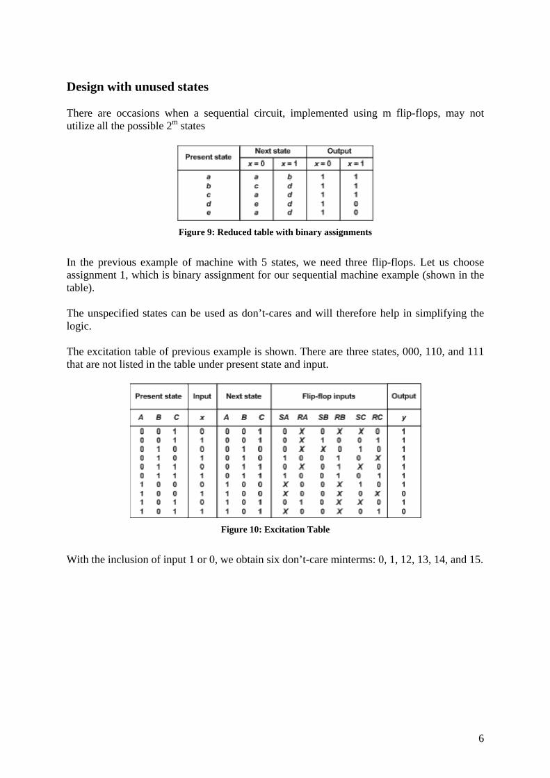
In the previous example of machine with 5 states, we need three flip-flops. Let us choose assignment 1, which is binary assignment for our sequential machine example (shown in the table). The unspecified states can be used as don’t-cares and will therefore help in simplifying the logic. The excitation table of previous example is shown. There are three states, 000, 110, and 111 that are not listed in the table under present state and input.

Figure 10: Excitation Table

With the inclusion of input 1 or 0, we obtain six don’t-care minterms: 0, 1, 12, 13, 14, and 15.

6

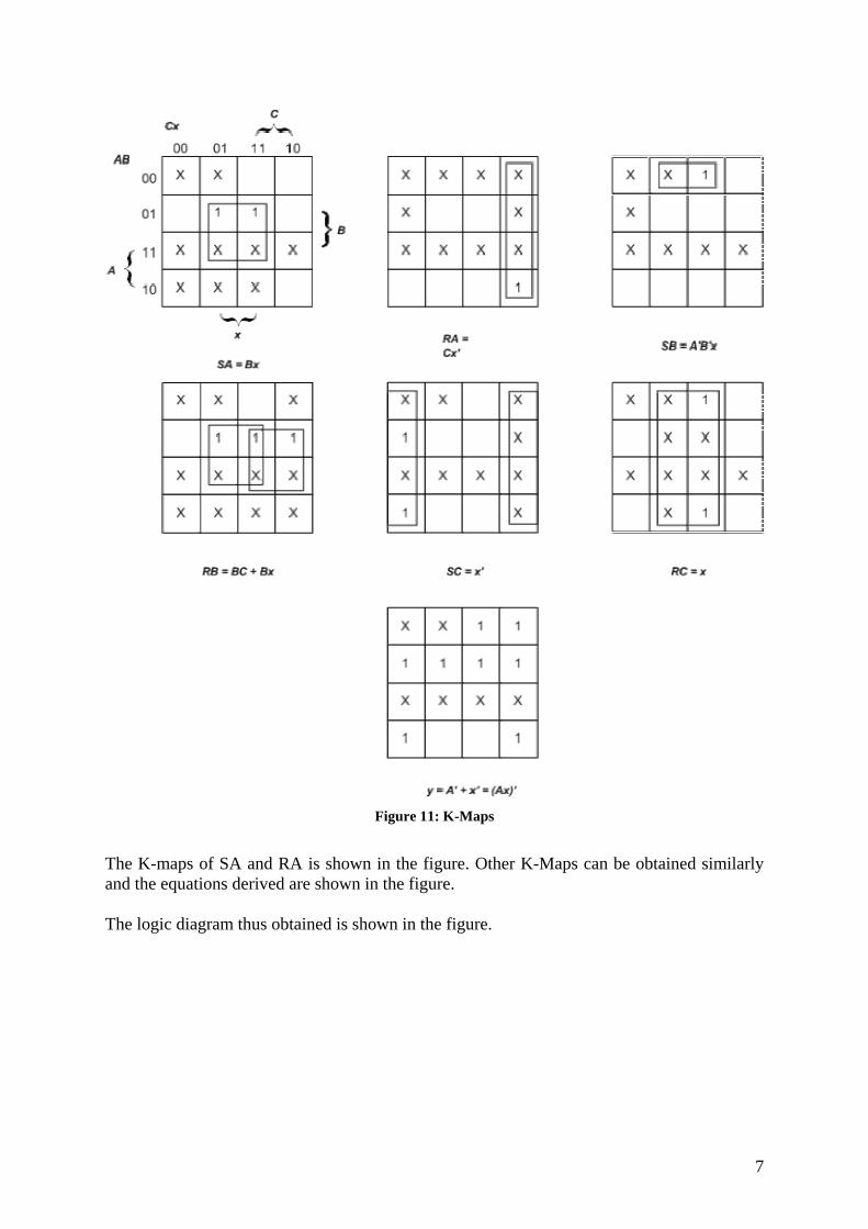
Figure 11: K-Maps

The K-maps of SA and RA is shown in the figure. Other K-Maps can be obtained similarly and the equations derived are shown in the figure. The logic diagram thus obtained is shown in the figure.

7

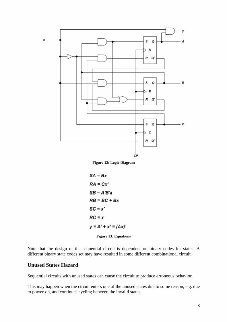
Figure 12: Logic Diagram

Figure 13: Equations

Note that the design of the sequential circuit is dependent on binary codes for states. A different binary state codes set may have resulted in some different combinational circuit. Unused States Hazard Sequential circuits with unused states can cause the circuit to produce erroneous behavior. This may happen when the circuit enters one of the unused states due to some reason, e.g. due to power-on, and continues cycling between the invalid states.

8

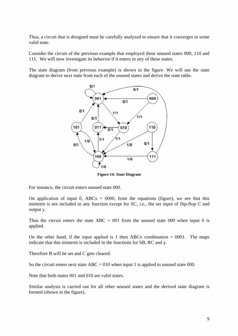
Thus, a circuit that is designed must be carefully analyzed to ensure that it converges to some valid state. Consider the circuit of the previous example that employed three unused states 000, 110 and 111. We will now investigate its behavior if it enters in any of these states. The state diagram (from previous example) is shown in the figure. We will use the state diagram to derive next state from each of the unused states and derive the state table.

Figure 14: State Diagram

For instance, the circuit enters unused state 000. On application of input 0, ABCx = 0000, from the equations (figure), we see that this minterm is not included in any function except for SC, i.e., the set input of flip-flop C and output y. Thus the circuit enters the state ABC = 001 from the unused state 000 when input 0 is applied. On the other hand, if the input applied is 1 then ABCx combination = 0001. The maps indicate that this minterm is included in the functions for SB, RC and y. Therefore B will be set and C gets cleared. So the circuit enters next state ABC = 010 when input 1 is applied to unused state 000. Note that both states 001 and 010 are valid states. Similar analysis is carried out for all other unused states and the derived state diagram is formed (shown in the figure).

9

We note that the circuit converges into one of the valid states if it ever finds itself in one of the invalid states 000, 110, and 111. Such a circuit is said to be self-correcting, free from hazards due to unused states.

10