Energy Conversion and Management 87 (2014) 754–764

Contents lists available at ScienceDirect

Energy Conversion and Management

journal homepage: www.elsevier .com/locate /enconman

Analysis and future outlook of natural gas consumption in the Italianresidential sector

http://dx.doi.org/10.1016/j.enconman.2014.07.0810196-8904/� 2014 Elsevier Ltd. All rights reserved.

⇑ Corresponding author. Tel.: +39 010 353 28 72.E-mail addresses: vincenzo.bianco@unige.it, vbianco@libero.it (V. Bianco).

Vincenzo Bianco ⇑, Federico Scarpa, Luca A. TagliaficoUniversity of Genoa – DIME/TEC, Division of Thermal Energy and Environmental Conditioning, Via All’Opera Pia 15/A, 16145 Genova, Italy

a r t i c l e i n f o

Article history:Received 30 May 2014Accepted 28 July 2014

Keywords:Energy consumptionNatural gasEnergy efficiencyForecasting

a b s t r a c t

The aim of the present paper is to evaluate the future consumption of natural gas in the Italian residentialsector. The historical pattern of the consumption is reported and analyzed in order to identify theconsumption drivers. It is found that natural gas consumption is influenced by gross domestic productper capita (GDP per capita), gas price and heating degree days (HDD); therefore an equation linking theseparameters is estimated by means of a linear regression analysis. The GDP per capita, gas price and HDDshort and long run elasticities of consumption have been estimated, showing that the larger influence isdue to HDD (i.e. climatic factor). On the basis of the evolution of the explaining variables, a ‘‘business asusual’’ (BAU) trend of consumption is estimated, showing that, in 2030, natural gas consumption in theresidential sector is expected to double that of 1990. Finally, the effect of energy saving measures in thesector of buildings heating is evaluated, showing that consumption might be reduced of �20% withrespect to BAU consumption, if the 15% of flats and 5% of single houses are properly insulated.

� 2014 Elsevier Ltd. All rights reserved.

1. Introduction

Italy is one of the main consumers of natural gas withinEuropean Union. With its total consumption of �69 bcm in 2012[1], it is the largest European consumer of natural gas after UKand Germany. Natural gas is widely utilized in Italy for differentpurposes such as industrial processes, offices heating, powergeneration and residential activities, in particular heating, cookingand sanitary water production.

Industrial and services, power generation and residentialsectors approximately present the same amount of consumption[2,3], therefore it is of paramount importance to study the evolu-tion of natural gas consumption in each of these three sectors, inorder to manage the future energy supply and the implementationof energy efficiency measures in a correct way.

The study of energy consumption models has attracted theinterest of many researchers, because primary energy demandhas been steadily growing for the last twenty years (+2.1% per yearfrom 1992 until 2012 [1]), but the resources to satisfy the demandare finite and an average increase of their price is regularlydetected (+6.5% per year for oil, +7.9% per year for natural gas,+4.5% per year for coal from 1992 until 2012 [1]). Anyway, it isto be mentioned that in the last years natural gas market has been

subjected to drastic changes, because a large oversupply isdetected on the European market due to the decrease of theinternal demand and to the utilization of shale gas in USA. In fact,USA was an importing country, but after the shale gas technicalbreakthrough they become an exporting countries and all theLNG which was supposed to be shipped to USA is now divertedtoward European and Asian markets, causing a strong oversupplywith a consequent decrease of prices.

Numerous researchers have analyzed various energy issues andfocused on developing appropriate energy demand models; but,while electricity demand has been the focus of the research com-munity, studies on natural gas demand modeling and forecastinghave not been reported in the scientific literature to the sameextent. In fact, quite recently different authors proposed interest-ing studies concerning the estimation of future natural gasconsumption in different countries, taking into account variouseconomic sectors and time horizons [3–10].

Sabo et al. [4] introduced an analytical model to predict naturalgas consumption in Croatia. Their analysis is referred to the shortterm prediction (i.e. hourly) of natural gas demand by introducingmodels with linear and nonlinear functions. These functions corre-late the expected future consumption to the past consumption andto the historical and forecasted temperature data. The model issuccessfully validated on historical data. Such a kind of model isuseful for the operation of gas distribution network (i.e. to imple-ment sophisticated control strategies) or to support energy traders

Nomenclature

A surface, m2

C natural gas consumption, bcmGDP gross domestic product, bn€HDD heating degree days, �Ci thermal dispersing element indexLE_GDPPC long run elasticity of consumption with respect to GDP

per capitaLE_HDD long run elasticity of consumption with respect to

HDDLE_Pres long run elasticity of consumption with respect to

pricek year indexm number of thermal dispersing elementsn number of yearsPres natural gas price for residential customer, €/GJ HHVPgas import price of natural gas, $/MbtuPoil oil price, $/bblQ heating demand, kWh m�2

U thermal conductance, W m�2 K�1

WAC weather adjusting coefficient

Greek Lettersa regression coefficientb1 short run elasticity of consumption with respect to

HDD

b2 short run elasticity of consumption with respect to Pres

b3 short run elasticity of consumption with respect toGDP per capita

b4–5 regression coefficientsc ratio between area of heat exchange toward external

environment of i-th elements and floor areav thermal dispersing surface ratiog global efficiency of heating system

Subscriptsavg averagee estimatedh heatingi refers to the i-th heat exchange surfacepc per-capitares residentialt refers to year ‘‘t’’

V. Bianco et al. / Energy Conversion and Management 87 (2014) 754–764 755

on real time markets. Similarly, Soldo et al. [5] studied the influ-ence of solar radiation on forecasting residential natural gas con-sumption. They proposed various forecasting models, linear andnon-linear, with one day ahead forecasting horizon, showing thatsolar radiation clearly influences natural gas consumption.

Tas�pinar et al. [6] presented a multilayer artificial neural net-work model with time series approach to forecast short-term nat-ural gas consumption in the Sakarya province in Turkey. By meansof this methodology, they were able to correlate natural gas con-sumption to meteorological parameters, which are identified asthe main driver of consumption in the short run.

Sánchez-Úbeda and Berzosa [7] proposed a model to forecastnatural gas consumption in the Spanish industrial sector. They con-sidered a longer forecasting horizon with respect to [3–6], in facttheir model is intended to forecast natural gas consumption inthe medium term (i.e. one-three years) with daily forecasting res-olution. Their approach is based on the decomposition methodol-ogy, according to which the historical series of consumption isbroken in a series of sub-series (i.e. the subseries of the Mondayvalues, the time subseries of the Tuesday values, and so forth)and each sub-series is modeled independently. In particular, eachsub-series is split into two parts: the irregular (i.e. random) anddeterministic components. The irregular component is assumedto be white noise, whereas the deterministic component is deter-mined as a function of weather and socio-economic variables, suchas HDD, wind speed, humidity, GDP, and population. The mainapplications of this model are in the field of market operations,in particular as a support tool for the forecasting of spot and futureprices, or in the area of network management, where it is funda-mental to study the future balance between demand and supply[7].

Forouzanfar et al. [8] studied natural gas consumption of theIranian commercial and residential sector by using a logistic basedapproach in combination with non-linear programming andgenetic algorithms. They used a historical series of ten years tobuild a model to predict the consumption three years ahead. This

model utilizes only the historical consumption of natural gas asinput, therefore it is not possible to study the effect that otherparameters, such as GDP, population, and climatic data, have onthe consumption. For this reason, it is suitable to forecast the con-sumption in the short or medium term, where it is assumed a lim-ited variation of the above mentioned factors.

Huntington [9], instead, further extend the horizon of the anal-ysis and proposed a statistical model based on regression analysisto forecast natural gas consumption in the USA industrial sectorover a period of twenty years. Natural gas consumption is esti-mated as a function of natural gas price, distillate oil price, heatingdegree days and natural gas consumption of the previous year. Themain purpose of this model is to help policy and corporate plan-ners to analyze important factors that could influence future trendsof consumption in the industrial sector.

Similarly, Li et al. [10] proposed a model to forecast long termconsumption of natural gas in China. They utilized a systemdynamics model to create a possible outlook and show that inthe future the consumption will increase and there will be a ‘‘coalto gas’’ substitution.

It can be noticed that the models presented in [3–10] refer todifferent forecasting horizon, therefore they utilize different mod-eling strategies.

Despite of the fundamental importance of energy supply in Italyand the central role of natural gas in the Italian energy mix, the sci-entific literature on these topics is rather scarce and only a fewpapers are available [3,11–13].

Bianco et al. [11,12] proposed two studies on the forecasting ofelectricity demand, whereas Gori and Takanen [13] introduced aneconometric model to forecast energy demand in Italy by takinginto account also inter-fuels substitution. These papers discussthe effect of some relevant variables, namely GDP, electricity priceand population, on the future consumption and provide ‘‘ready touse’’ models to estimate future outlooks.

Very recently, Bianco et al. [3] analyzed nonresidential gas con-sumption in Italy and suggested a scenarios approach to take into

756 V. Bianco et al. / Energy Conversion and Management 87 (2014) 754–764

account the impact of the variation of the considered consumptiondrivers, namely GDP per capita, natural gas price and minimumtemperature. With reference to the evolution of the consumptiondrivers, different scenarios are analyzed, in order to quantify thevariation of the consumption in the case of specific events (i.e. coldwinter, low oil price, high GDP growth and so on).

A comprehensive review of the literature on energy models fordemand forecasting can be found in Suganthi and Samuel [14] andSoldo [15]. In particular, reference [15] is devoted to the forecast-ing of natural gas consumption.

Forecasting of energy demand is gaining importance, becausesome countries (i.e. EU) have started to support the reduction ofprimary energy consumptions by promoting energy efficiency pol-icies, therefore it is necessary to set up appropriate saving mea-sures, in order to reach the proposed target and, to do this, anaccurate prediction of future consumption is mandatory.

In the last years, EU focused on the energy efficiency in build-ings; in fact, two important directives on this topic, namely2010/31/EU [16] and 2012/27/EU [17], were emanated.

Buildings are considered as a sector which offers considerablepossibilities for energy savings, in fact the Directive 2010/31/EUis specifically devoted to them. It establishes a series of specificminimum requirements in terms of consumption for various clas-ses of buildings and introduced a mechanism of certification inorder to assess their energy performance. Moreover, the directivealso imposes to the member states to develop the National Effi-ciency Action Plan, where it is explained how to reach the energyefficiency targets.

The Directive 2012/27/EU on energy efficiency [17] strengthensthe fact that there is a relevant potential to reduce primary energyconsumption in buildings and, therefore, the residential sector isconsidered one of the strategic areas to reach the EU target ofthe reduction of 20% of primary energy consumption in 2020. Tostimulate the implementation of energy efficiency measure inbuildings, the directive set a mandatory target on the buildingsowned and occupied by the central government. In fact, it is pre-scribed that each year the 3% of the surface of these buildings haveto meet, at least, the minimum energy performance requirementsin accordance with Article 4 of Directive 2010/31/EU.

Italy, in quality of EU member, is obliged to be compliant withthe above mentioned directives, therefore a National EfficiencyAction Plan (NEAP) is available [18], where it is reported the pro-posed strategy to achieve the efficiency target. As observed in[19], Italian NEAP [18] reports some information regarding thefinancial support on actions to enhance energy performance of res-idential buildings, but there is a lack on the long term strategy andexperts are comparatively critical toward the Italian policy pack-age, which is considered inconclusive (i.e. there is not an estima-tion of the absolute saving) and concerns are expressed regardingthe achievement of the national efficiency target [19].

It is authors’ opinion that in order to study the feasibility of anyefficiency target, it is necessary to estimate the future consumptionin a ‘‘business as usual’’ (BAU) scenario and then to analyze thepotential impact of possible efficiency measures.

The object of the present paper is to analyze residential naturalgas consumption in Italy, estimating the consumption equation bymeans of a linear regression model, in order to perform a forecast-ing of future consumption on the basis of significant explainingvariables. The second target is to analyze the impact of some effi-ciency measures on future consumption, in order to assess the pos-sibility to achieve a saving of about 20% with respect to the BAUconsumption level.

It is believed that the information contained in this paper is use-ful for energy managers and policy makers, in order to designappropriate supply/consumption strategies and energy policies.

For example the knowledge of price elasticities helps the dis-tributors to set up adequate pricing policies, whereas the projec-tions of consumption are important to pursue correct supplystrategies.

2. Description of data series

In order to develop the forecasting model, different data seriesare necessary. The data series considered in the present analysisare: population, gross domestic product (GDP), heating degreedays (HDD), natural gas consumption in the residential sectorand its price.

All the data range from 1990 up to 2012 and they are takenfrom official sources, freely available on line [2,20,21]. Table 1summarizes the data and all the respective sources.

2.1. Economic and climatic data

Fig. 1(a) shows the trend of GDP and GDP per capita (i.e. theratio between GDP and population) and it highlights that from1990 up to 2008, a nearly linear growth trend can be observed,whereas from 2008 up 2012 a fluctuating behavior is detected,mainly due to the economic downturn.

Fig. 1(b) displays the population profile, showing an interestingpattern, where there is practically no growth from 1990 up to 2000and then a linear growth trend is detected. The first part of the pro-file maybe explained with the fact that between 1990 and 2000there was an equilibrium between birth rate and death rate caus-ing the stability of population, whereas from 2000 onward thegrowth of the population is mainly explained with immigrationfrom other countries [11,12].

Fig. 1(c) shows the price of residential natural gas in Italy. Anirregular pattern is detected from the figure, which is mainlylinked to the fluctuations of the oil market, because natural gasprice and oil price are strictly connected as discussed in [3]. More-over, natural gas prices for final users incorporates different kindsof taxations imposed by the Italian authorities, therefore the priceis influenced also by tax policies, which varies in the time.

Fig. 1(d) reports the historical series of HDD, which are to beconsidered as a proxy of climatic conditions. They are of relevantimportance, because the level of usage of heating systems dependson HDD value, therefore they influence a large share of natural gasconsumption in the Italian residential sector.

2.2. Analysis and historical evolution of residential natural gasconsumption

Fig. 2(a) reports the historical trend, from 1990 up to 2012, ofnatural gas consumption in the residential sector. It can beobserved that many fluctuations are present in the consumptionpattern and they are largely due to the variation of the climaticconditions year by year.

In order to filter climatic effects, data have been ‘‘weatheradjusted’’ to highlight any possible trend not dependent from cli-matic conditions.

To adjust the consumption data, the methodology suggested in[22] is applied. It consists in the calculation of a coefficient on thebasis of the actual and historical average of the HDD:

WACt ¼ HDDavg=HDDt ð1Þ

HDDavg represents the average value of the heating degree daysof the considered period (i.e. 1990–2012, as reported in Fig. 1(d)),whereas HDDt represents the value of heating degree days in yeart. By applying Eq. (1), it is possible to obtain the weather adjustingcoefficient (WAC) for each year and, thus, by multiplying WACt for

Table 1Sources of historical data used in the analysis.

Variable Years Source

Natural gas consumption 1990–2011 European statistical office (Eurostat) [2]Natural gas consumption 2012 Italian ministry of economic development [20]Natural gas price 1990–2012 Eurostat [2]Gross domestic product (GDP) 1990–2012 Italian statistical office (ISTAT) [21]Population 1990–2012 ISTAT [21]Heating degree days 1990–2012 European statistical office (Eurostat) [2]

Fig. 1. Historical series of relevant variables for Italy: (a) gross domestic product, (b) population, (c) gas price for residential customers and (d) heating degrees days.

V. Bianco et al. / Energy Conversion and Management 87 (2014) 754–764 757

the consumption in year t, it is possible to get the weather adjustedconsumption. Data reported in Fig. 1(d) represent the official HDDsvalue for Italy, as given in [2]. Of course it can be noticed that theyare a country average, because Italy, due to its particular geograph-ical morphology, has very different climatic areas (i.e. from Alpineto Mediterranean climates), where huge differences in terms ofHDDs are detected (i.e. from �4000 HDDs in Trentino to �1000HDDs in Sicily).

Weather adjusted consumption of residential natural gas isshown in Fig. 2(a). It highlights a steady growth of consumptionsfrom 1990 until the beginning of 2000s. This trend is to beexplained according to the energy policy pursued in Italy; in fact,in those years there was the development of a very efficient andwidespread natural gas distribution network. The availability ofsuch a network pushed residential users to utilize natural gas tofuel their heating systems, rather than heating fuel oil or gasoil.In fact, heating fuel oil/gasoil consumption represented the 29%of the total (calculated on the basis of weather adjusted data) in2001 versus the 45% of 1990, whereas natural gas consumptionrepresented the 71% of the total in 2001 versus the 55% of 1990[2]. Therefore, it can be said that in those years the fuel switchingplayed an important role in the increase of natural gas consump-tion in the residential sector. After 2001, the consumption resultsto be stable around 20.5 bcm (weather adjusted), with a slightlyincreasing trend.

Most of the utilization of natural gas in the residential sector,�82%, is due to space heating, whereas sanitary water accountsfor �11% and the remaining part, �7%, is represented by consump-tion for cooking [20]. These shares were substantially stable in theperiod 1990–2012.

Fig. 2(b) reports the patterns of energy intensity per capita (i.e.the ratio between gas consumption in the residential sector andthe population), in the case of ‘‘raw’’ and ‘‘weather adjusted’’ data.The figure highlights that temperature effects are relevant, in fact,‘‘raw’’ energy intensity data are characterized by strong fluctua-tions, whereas the weather adjusted data show a more regularpattern.

Weather adjusted energy intensities follow a trend similar tothe consumption, with a strong increase from 1990 up to thebeginning of 2000s, but afterwards a more regular behavior isobserved, with a slight decrease in the last four years.

3. Methodology

3.1. Estimation of the forecasting model

In order to estimate future consumption of natural gas in theItalian residential sector, it is necessary to build an equation whichlinks all the relevant variables. In the following, it is proposed an

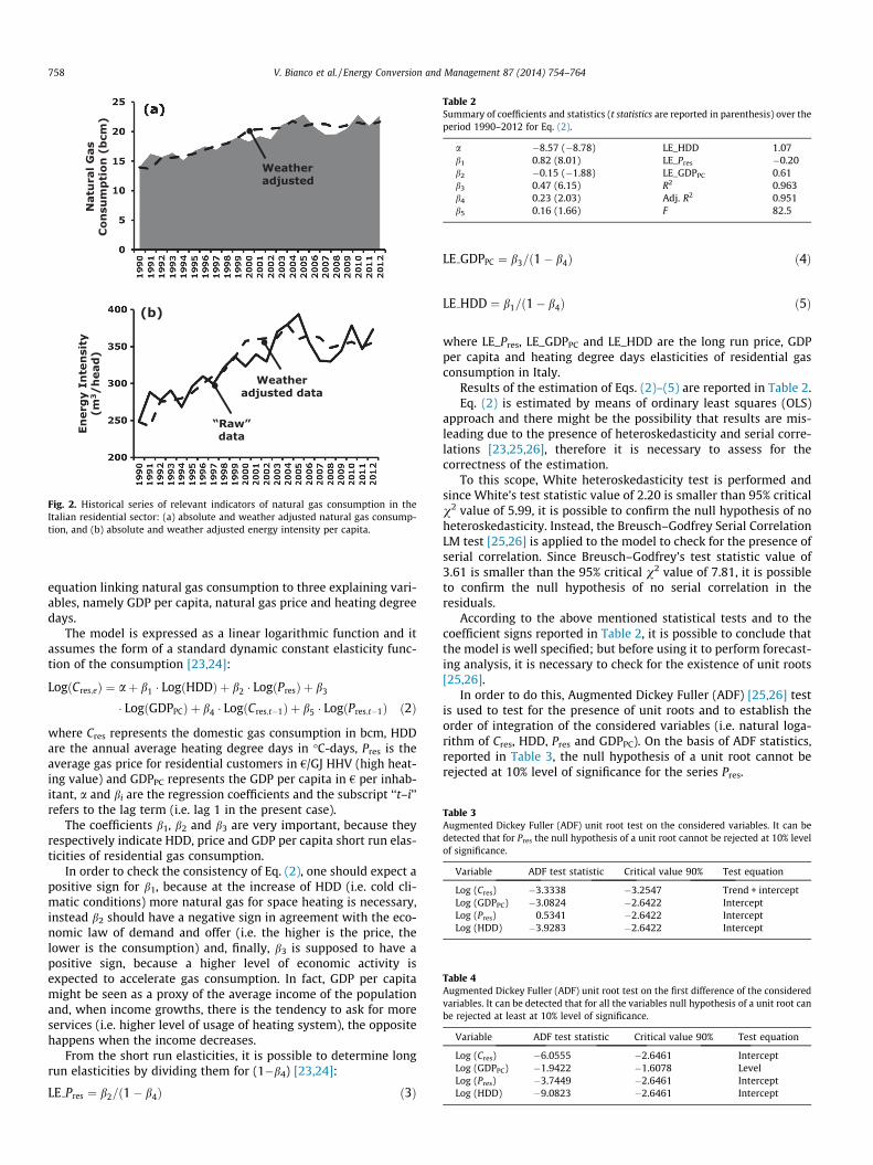
Fig. 2. Historical series of relevant indicators of natural gas consumption in theItalian residential sector: (a) absolute and weather adjusted natural gas consump-tion, and (b) absolute and weather adjusted energy intensity per capita.

Table 2Summary of coefficients and statistics (t statistics are reported in parenthesis) over theperiod 1990–2012 for Eq. (2).

a �8.57 (�8.78) LE_HDD 1.07b1 0.82 (8.01) LE_Pres �0.20b2 �0.15 (�1.88) LE_GDPPC 0.61b3 0.47 (6.15) R2 0.963b4 0.23 (2.03) Adj. R2 0.951b5 0.16 (1.66) F 82.5

Table 3Augmented Dickey Fuller (ADF) unit root test on the considered variables. It can bedetected that for Pres the null hypothesis of a unit root cannot be rejected at 10% levelof significance.

Variable ADF test statistic Critical value 90% Test equation

Log (Cres) �3.3338 �3.2547 Trend + interceptLog (GDPPC) �3.0824 �2.6422 InterceptLog (Pres) 0.5341 �2.6422 InterceptLog (HDD) �3.9283 �2.6422 Intercept

Table 4Augmented Dickey Fuller (ADF) unit root test on the first difference of the consideredvariables. It can be detected that for all the variables null hypothesis of a unit root canbe rejected at least at 10% level of significance.

Variable ADF test statistic Critical value 90% Test equation

Log (Cres) �6.0555 �2.6461 InterceptLog (GDPPC) �1.9422 �1.6078 LevelLog (Pres) �3.7449 �2.6461 InterceptLog (HDD) �9.0823 �2.6461 Intercept

758 V. Bianco et al. / Energy Conversion and Management 87 (2014) 754–764

equation linking natural gas consumption to three explaining vari-ables, namely GDP per capita, natural gas price and heating degreedays.

The model is expressed as a linear logarithmic function and itassumes the form of a standard dynamic constant elasticity func-tion of the consumption [23,24]:

LogðCres;eÞ ¼ aþ b1 � LogðHDDÞ þ b2 � LogðPresÞ þ b3

� LogðGDPPCÞ þ b4 � LogðCres;t�1Þ þ b5 � LogðPres;t�1Þ ð2Þ

where Cres represents the domestic gas consumption in bcm, HDDare the annual average heating degree days in �C-days, Pres is theaverage gas price for residential customers in €/GJ HHV (high heat-ing value) and GDPPC represents the GDP per capita in € per inhab-itant, a and bi are the regression coefficients and the subscript ‘‘t–i’’refers to the lag term (i.e. lag 1 in the present case).

The coefficients b1, b2 and b3 are very important, because theyrespectively indicate HDD, price and GDP per capita short run elas-ticities of residential gas consumption.

In order to check the consistency of Eq. (2), one should expect apositive sign for b1, because at the increase of HDD (i.e. cold cli-matic conditions) more natural gas for space heating is necessary,instead b2 should have a negative sign in agreement with the eco-nomic law of demand and offer (i.e. the higher is the price, thelower is the consumption) and, finally, b3 is supposed to have apositive sign, because a higher level of economic activity isexpected to accelerate gas consumption. In fact, GDP per capitamight be seen as a proxy of the average income of the populationand, when income growths, there is the tendency to ask for moreservices (i.e. higher level of usage of heating system), the oppositehappens when the income decreases.

From the short run elasticities, it is possible to determine longrun elasticities by dividing them for (1�b4) [23,24]:

LE Pres ¼ b2=ð1� b4Þ ð3Þ

LE GDPPC ¼ b3=ð1� b4Þ ð4Þ

LE HDD ¼ b1=ð1� b4Þ ð5Þ

where LE_Pres, LE_GDPPC and LE_HDD are the long run price, GDPper capita and heating degree days elasticities of residential gasconsumption in Italy.

Results of the estimation of Eqs. (2)–(5) are reported in Table 2.Eq. (2) is estimated by means of ordinary least squares (OLS)

approach and there might be the possibility that results are mis-leading due to the presence of heteroskedasticity and serial corre-lations [23,25,26], therefore it is necessary to assess for thecorrectness of the estimation.

To this scope, White heteroskedasticity test is performed andsince White’s test statistic value of 2.20 is smaller than 95% criticalv2 value of 5.99, it is possible to confirm the null hypothesis of noheteroskedasticity. Instead, the Breusch–Godfrey Serial CorrelationLM test [25,26] is applied to the model to check for the presence ofserial correlation. Since Breusch–Godfrey’s test statistic value of3.61 is smaller than the 95% critical v2 value of 7.81, it is possibleto confirm the null hypothesis of no serial correlation in theresiduals.

According to the above mentioned statistical tests and to thecoefficient signs reported in Table 2, it is possible to conclude thatthe model is well specified; but before using it to perform forecast-ing analysis, it is necessary to check for the existence of unit roots[25,26].

In order to do this, Augmented Dickey Fuller (ADF) [25,26] testis used to test for the presence of unit roots and to establish theorder of integration of the considered variables (i.e. natural loga-rithm of Cres, HDD, Pres and GDPPC). On the basis of ADF statistics,reported in Table 3, the null hypothesis of a unit root cannot berejected at 10% level of significance for the series Pres.

Table 6Comparative analysis of forecasting errors.

Errormeasure

Eq. (2) Energy intensityforecasting

Simple linear fitforecasting

MAPE 0.6% 2.7% 3.81%MAD 0.108 bcm 0.585 bcm 0.792 bcmMSE 0.309 bcm2 0.365 bcm2 1.390 bcm2

RMSE 0.556 bcm 0.604 bcm 1.179 bcm

V. Bianco et al. / Energy Conversion and Management 87 (2014) 754–764 759

In light of this, the ADF test is executed on the first difference ofthe variable, indicating that the series Pres is integrated of order 1,I(1) in nature. As given in [23,25–27] if, after running the ADF teston the first difference of the considered variables, stationarity isobtained, then Eq. (2) may be regarded as a valid long run equilib-rium relation, if the resulting residuals are stationary, I(0).

Table 4 shows the ADF test on the first differences of all the con-sidered variables, confirming that they are stationary and the ADFtest performed on the residuals, known as AEG (Augmented EngleGranger) [28], of Eq. (2) confirms that they are I(0). Therefore, itcan be concluded that the variables are co-integrated and the esti-mated equation may be considered as a valid expression to forecastgas consumption [28].

3.2. Error analysis and model validation

In order to verify the modeling and prediction accuracy of Eq.(2) an error analysis is developed. To measure the performanceof the proposed model four error indicators are taken into account,namely mean absolute percentage error (MAPE), mean absolutedeviation (MAD), mean square error (MSE) and root mean squareerror (RMSE) [29].

MAPE is a percentage measure of the prediction accuracy,whereas MAD and MSE are two indicators of the average magni-tude of absolute forecasted errors, but the latter imposes a greaterpenalty on a large error rather than several small deviations andRMSE is a measure of the average distance of estimated pointsfrom the real data. As MSE, RMSE is mostly influenced by largeerrors. The four indicators are defined as follows:

MAPE ð%Þ ¼ 1n

Xn

k¼1

Cres;eðkÞ � CresðkÞ�� ��

CresðkÞð6Þ

MAD ¼ 1n

Xn

k¼1

Cres;eðkÞ � CresðkÞ�� �� ð7Þ

MSE ¼ 1n

Xn

k¼1

ðCres;eðkÞ � CresðkÞÞ2 ð8Þ

RMSE ¼

ffiffiffiffiffiffiffiffiffiffiffiffiffiffiffiffiffiffiffiffiffiffiffiffiffiffiffiffiffiffiffiffiffiffiffiffiffiffiffiffiffiffiffiffiffiffiffiffiffiffiffiffiffi1n

Xn

k¼1

ðCres;eðkÞ � CresðkÞÞ2vuut ð9Þ

To validate the model, Eq. (2) is estimated on data ranging from1990 up to 2008, thus the remaining four years (i.e. 2009–2012)are utilized for the model validation on new data.

In this way, it is possible to establish the forecasting accuracy ofthe proposed approach.

It is important to notice that the coefficients of the equationestimated on such time horizon are slightly different from thosereported in Table 2, because years 2009–2012 are now excludedfrom the estimation.

For comparison purposes two simpler forecasting models arealso implemented. One is represented by the simple linear fittingof the consumption over time (i.e. 1990–2008), whereas the otherone is based on the energy intensity. In particular, the average

Table 5Observed and forecasted natural gas consumption. Relative errors (RE) are repor

Year Observed values (bcm) Eq. (2) Forecasting (bcm) Ener

2009 20.5 20.8 (+1.5%) 21.12010 22.8 22.5 (�1.6%) 23.32011 21.0 21.9 (+4.3%) 21.82012 22.7 22.3 (�1.8%) 23.2

energy intensity per capita of the last five years (i.e. 2004–2008)is taken into account and total consumption is obtained by multi-plying this value for the population.

This testing procedure allows to validate the model and to jus-tify the modeling effort.

Table 5 reports the estimations based on the above mentionedmethodologies and it shows that straight line fitting is not ade-quate to forecast residential natural gas consumption, whereasthe other two methods result to be more appropriate.

In support of this conclusion, Table 6 shows the error indicatorsfor all the three forecasting approaches taken into account and ithighlights that Eq. (2) furnishes the most accurate results, whereasthe linear fitting presents higher deviations, instead the energyintensity methodology has a satisfactory level of accuracy, espe-cially if compared to the simplicity of the method, but it is lessaccurate than Eq. (2).

Therefore, it can be concluded that Eq. (2) represents a valid andsufficiently accurate approach to forecast natural gas consumptionin the Italian residential sector.

4. Projection of the consumption drivers

In order to forecast the residential natural gas consumption, it isnecessary to have a future outlook of the explaining variables uti-lized in Eq. (2), namely GDP per capita, natural gas price and HDD.

The outlook of GDP per capita is built by utilizing the projec-tions of population growth, Fig. 3(a), given in [21] and the expectedGDP trend reported in [30]; thus the evolution of GDP per capita isobtained, Fig. 3(b).

The GDP growth rates given in [30] are in real values and to getnominal values a consumer price index (CPI) of 2.1% is hypothe-sized, corresponding to the average of the CPI in the last ten years(i.e. 2003–2012) [17].

As for the natural gas price, a correlation between BAFA gasprice (i.e. gas prices published by the German Federal Office of Eco-nomics and Export Control) and oil price is studied.

BAFA price is considered as a reference for the EU market; itrepresents an average of the German oil indexed gas supply con-tracts. In the last years other price references aroused in EU (i.e.liquid gas hubs such as NBP, TTF and Zee), but BAFA is consideredto be a valid reference for this study for two main reasons.

The first one consists in the fact that the largest share of gas istransacted on the basis of oil indexed long term contracts of whichBAFA is considered a good proxy at EU level.

The second reason is represented by the fact that the elasticityof gas consumption in the residential sector with respect to the

ted in parenthesis.

gy intensity forecasting (bcm) Simple linear fit forecasting (bcm)

(+2.9%) 22.0 (+7.2%)(+1.9%) 22.4 (�2.0%)(+3.9%) 22.8 (+8.3%)(+2.1%) 23.1 (+1.7%)

Fig. 3. Projections of population (a) and gross domestic product (b) for Italy.

Fig. 4. Projections of energy price: (a) correlation between BAFA long term contractand oil price, (b) outlook of oil price, and (c) forecasting of import and final user gasprice for Italian customers.

760 V. Bianco et al. / Energy Conversion and Management 87 (2014) 754–764

price is quite limited, therefore a variation of the average price, dueto the effect of hubs pricing mechanisms, causes a modest reactionin terms of consumption.

As shown in Fig. 4(a), historical prices of BAFA and oil arestrongly related to each other and a linear correlation is deter-mined. Thus, to estimate future natural gas price, oil price projec-tions given in [31] are considered, Fig. 4(b).

Fig. 4(c) reports natural gas price projections, hypothesizingthat the cost of the commodity will represent the 33% [32] of thefinal user price for residential customers, in accordance with thehistorical average.

Finally, it is necessary to make an assumption on the expectedHDDs scenario. For the sake of simplicity three scenarios of HDDsare considered. In particular, a first scenario considers the averageHDDs from 1990 up to 2012, 1879 �C-days, and it is representativeof average weather conditions. Whereas the other two consideredscenarios can be considered as ‘‘extreme’’, because in one case theminimum HDDs from 1990 up to 2012, 1695 �C-days, and in theother case maximum HDDs, 2234 �C-days, are taken into account.In this way, it is possible to give the best estimation of reasonableminimum and maximum amount of consumption.

5. Energy efficiency measures

Italian residential sector has a huge potential to decrease theconsumption of natural gas. Main opportunities to implementenergy efficiency measures are available in the field of space heat-ing, which represents the main source of consumption, accountingfor �82% of natural gas consumption. This incidence is assumed tobe kept constant also for the future, because the historical trendshows that it was practically constant from 1990 until 2012.

The consumption of natural gas for heating purposes can beestimated in the following way for a generic dwelling:

Qh ¼24

1000�Xm

i¼1

vi � Ui �HDDg

ð10Þ

where Q is the heating demand in kWh/m2 per year, vi and Ui arethe ‘‘thermal dispersing surface ratio’’ and heat transfer coefficientof thermal dispersing elements, whereas g is the global efficiencyof the heating system. vi is a non-dimensional quantity, called‘‘thermal dispersing surface ratio’’ and it is defined as:

vi ¼ciPni¼1ci

ð11Þ

where ci is the non-dimensional area of heat exchange of the i-thdispersing elements (i.e. walls, windows, etc.) toward the externalenvironment:

ci ¼Ai

Afloorð12Þ

In the present paper dispersions through external walls, win-dows, floor and roof are taken into account.

Table 7Construction characteristics of the two considered classes of buildings. The flat is assumed to belong to a building block of 5 floors with 4 apartments per floor [33–35].

Variable Flat Singlehouses

Assumptions

Flat Single houses

Wall tobuildingfootprintratio

c = 0.62 c = 1.10 Assumed that two of the four dwelling walls exchange heatwith the external environment. As reference data, it can beassumed a net surface of�90 m2 and walls height of 3 m [33]

Assumed that all the four walls exchange heat with theexternal environment As reference data, it can be assumed anet surface of �120 m2 and walls height of 3 m [33]

v = 50.8% v = 33.3%

Windows tobuildingfootprintratio

c = 0.20 c = 0.20 Windows represent 20% of the dwelling surface according to common construction practice in Italyv = 16% v = 6.1%

Roof tobuildingfootprintratio

c = 0.20 c = 1.00 An equivalent floor surface per apartment is calculated bydividing the total floor surface for the number of apartments(e.g. 20)

Roof surface equal to building footprintv = 16% v = 30.3%

Floor tobuildingfootprintratio

c = 0.20 c = 1.00 Same hypothesis as ‘‘roof to building footprint ratio’’ Floor surface equal to building footprintv = 16% v = 30.3%

Totalequivalentthermaldispersingsurface

c = 1.22 c = 3.30v = 100% v = 100%

Table 8U values for existing residential buildings in Italy. Data are determined on the basis ofvalues reported in [34,35].

Building element Flat Single house

Ui

(W/(m2 K))Ui�vi

(W/(m2 K))Absolutevalue

Equivalentvalue

Walls 0.98 0.50 0.76 0.25Windows 3.40 0.56 3.40 0.21Roof 1.70 0.28 0.95 0.29Floor 1.24 0.20 0.98 0.30

V. Bianco et al. / Energy Conversion and Management 87 (2014) 754–764 761

To estimate the specific energy (i.e. per square meter) demandfor heating, the building stock is divided in two main categories,namely flats and single houses. According to [33], the 75% of dwell-ings is represented by flats and 25% by single houses; these sharesare supposed to be constant for all the analysis horizon.

Tables 7 and 8 report the specific characteristics of the two clas-ses of buildings considered in the present paper.

The implementation of energy efficiency measures have thescope to reduce the value of U, which means to increase the ther-mal resistance of walls, windows, floor and roof; for example, byintroducing an optimized insulation layer [36]. In order to beimplemented, such measures must be cost effective and the moreconvenient they are, the higher is their implementation rate.

By means of Eq. (10), it is possible to calculate the specific sav-ings of gas consumption due to the implementation of energy effi-ciency measures and thus it is possible to estimate the amount ofenergy saving as a function of the implementation rate. For exam-ple, it can be determined how much should be the implementationrate in order to reach a determined energy saving target.

6. Results and discussion

6.1. Estimated elasticities and expected consumption

To analyze the structure of natural gas consumption in theresidential sector, Eq. (2) is built and it is found that residentialconsumption of natural gas is affected by GDP per capita, usersprice and climatic factors (i.e. HDDs in the present study).

The long term elasticities of all the explaining variables, namelyLE_Pres, LE_GDPPC, and LE_HDDs, have been determined and theyassume the following respective values �0.1993, 0.6090 and1.0659.

The expected signs of elasticities seem to be consistent; in factlong run price elasticity has a negative sign in agreement with thefact that at the increase of price corresponds a decrease of con-sumption, whereas GDP per capita has a positive elasticityexplained by the fact that a higher level of economic activity andspending capacity tends to stimulate consumption and, finally, atthe increase of HDDs (i.e. more rigid climatic conditions) corre-sponds a growth of consumption.

As for the values of the elasticities, it can be observed thatLE_Pres has the lowest absolute value, showing that price variationshave a limited impact on consumption (i.e. gas consumption isinelastic to price). This can be explained with the fact that the tech-nical options to react to the increase of price are quite limited, infact only two possible solutions appear to be realistic: the imple-mentation of energy efficiency measures (i.e. improvement ofbuilding insulation, reduction of ventilation losses, etc.) or the sub-stitution of the primary fuel of the heating plant.

However, the implementation of these measures has a cost anduntil the price level does not make them financially convenient,with a short pay-back period, they are not taken into account.

It should be observed that the evaluation of these investmentsis rather complex, because natural gas price is fluctuating, there-fore it is difficult to understand if a variation in price is due to arandom phenomenon or to a structural change that will last inthe time, making possible an investment [3].

This situation is analogous to that of the residential electricitysector, as reported in [11].

As for LE_GDPPC, it has a higher absolute value with respect toLE_Pres, but less than LE_HDD. LE_GDPPC shows that at the increaseof the GDP per capita, which might be regarded as a proxy of thespending capacity per capita, corresponds an increase of the con-sumption. This means that at the increase of their spending capac-ity, users are encouraged to consume more, rather than investingin energy saving. Therefore, to promote energy saving policies, itis necessary to stimulate the users by encouraging a more efficientusage of primary energy resources, as is the case of EU [16,17],

Fig. 5. Forecasting of ‘‘business as usual’’ gas consumption in the Italian residentialsector as function of climatic conditions.

Fig. 6. Historical pattern and future outlook of weather adjusted consumption andenergy intensity for the Italian residential sector.

762 V. Bianco et al. / Energy Conversion and Management 87 (2014) 754–764

where a directive was emanated to set mandatory targets in termsof energy saving.

The analysis of elasticity values shows that LE_HDD has thehighest value. This means that climatic conditions strongly affectnatural gas consumption in the Italian residential sector.

This result can be explained by the fact that most of the naturalgas consumption is due to heating systems [20]. An increase ofHDDs provokes a large growth of natural gas consumption, which,in turn, may result in a complex practical management of the sup-ply network. In fact, climatic conditions are very difficult to beforecasted long time in advance with a relevant degree of accuracy,therefore it is necessary the utilization of a storage system to sat-isfy the sudden peak demand of gas determined by rigid climaticconditions.

The outlook of future natural gas consumption is reported inFig. 5, which shows the amount of natural gas consumed in threedifferent scenarios of yearly HDDs, namely ‘‘rigid’’ (2234 �C), ‘‘aver-age’’ (1879 �C) and ‘‘warm’’ (1695 �C), corresponding to rigid, aver-age and warm climatic conditions. The figure highlights that theimpact of HDDs is relevant, as already noticed by analyzing thelarge value of elasticity, and in the ‘‘rigid’’ scenario the consump-tion is about 20% higher with respect to the ‘‘average’’ one, whereasthe ‘‘warm’’ scenario presents consumptions about 10% lower withrespect to the ‘‘average’’ case. In terms of consumption, it meansthat if, for example, in 2030 there will be a rigid winter the con-sumption will result�6 bcm higher with respect to an average one.

The knowledge of this parameter is of fundamental importancefor supply network managers, because it represents a necessaryinput for the correct design of natural gas storages, which, as pre-viously stated, are necessary to manage unexpected conditions,such as rigid winter. On the contrary, a warm winter would leadto a decrease of consumption of �3 bcm in 2030.

These estimations might result of relevant importance also forcompanies involved in the supply of natural gas to residential cus-tomers, because in this way they can manage their position on themarket.

In fact, for example, suppliers know that, in the case of a warmwinter, the market will be long with respect to the average andthey necessitate a strategy to divert this quantity in excess towardother markets (i.e. other countries or other sectors). The oppositehappens in the case of cold winter.

Fig. 6 reports the historical pattern of weather adjusted con-sumption and the future outlook, showing that in 2030 theexpected consumption will double the consumption of 1990. Thismeans that natural gas will increase its importance as primaryenergy source in the residential sector, therefore it is necessaryto manage accurately its sourcing by adequately mixing all theavailable sources (i.e. pipelines, LNG, biogas, etc.) and to developan adequate infrastructure to guarantee the correct distributionto all the customers.

The figure also reports the trend of the energy intensity percapita, which is expected to double in 2030 with respect to 1990.

The outlook of the consumption of natural gas in the residentialsector and of its energy intensity per capita (Figs. 5 and 6) mayberegarded as ‘‘business as usual’’ (BAU) estimations.

In other words, they represent the projections of consumptionby assuming that the policies currently in place will be kept untilthe end of the forecasting period and users’ habits are extrapolatedon the basis of historical data, therefore the impact of new energypolicies and different users’ behavior is not taken into account.

6.2. Impact of energy efficiency measures

According to [16,17], EU has set the target of 20% of saving ofprimary energy in the building sector with respect to BAU projec-tion. In order to reach this target, it is necessary to implementenergy saving measures which contribute to reduce energyconsumption.

In this section it is discussed how the implementation of someefficiency measures, namely insulation of external walls, roof andfloor and substitution of windows, might allow to reach this targetfor the Italian residential sector.

Table 9 reports the main parameters of the energy efficiencymeasures taken into account.

By applying Eq. (10), assuming HDDs = 1879 �C and g � 80%[37], it is possible to estimate the specific energy consumptiondue to the considered measures, obtaining a value of 30 kWh/m2

per year in the case of flats and �26 kWh/m2 per year in the caseof single houses. These figures, according to the Italian LegislativeDecree 22/11/2012 [38], correspond to have flats with energy per-formance of class ‘‘B’’ (i.e. energy consumption between 31 and50 kWh/m2 per year) and single houses of class ‘‘A’’ (i.e. energyconsumption between 15 and 30 kWh/m2 per year).

To evaluate the convenience of such measures, the Net PresentValue (NPV) methodology is employed and the results are reportedin Table 10.

The cash flow stream for the NPV calculation is represented bythe value of the saving of primary energy (i.e. energy saving forspace heating multiplied by natural gas price), whereas the invest-ment is represented by the costs of installation of insulation sub-strates and of substitution of windows. Table 10 reports apositive NPV for a flat and a single house, therefore the implemen-tation of the proposed efficiency measures is cost effective, but thepayback period is quite long and this may discourage theinvestment.

If in 2020, the 15% of the flats and 5% of single houses imple-ment the measures reported in Table 9, the consumption of naturalgas for heating purposes in the Italian residential sector will bereduced of �21%. Furthermore, if in 2030 the 28% of flats and 9%

Table 9Main parameters of implemented energy measures on flats and single houses. Data are estimated on the basis of the values reported in [36].

External walls Windows Roof Floor

FlatInsulation thermal conductivity (W/(m K)) 0.04 n.a. 0.04 0.04Insulation thickness (cm) 2.0 n.a. 4.0 2.0Ui (W/(m2 K)) 0.66 2.71 0.62 0.76Ui�vi (W/(m2 K)) 0.33 0.44 0.10 0.12Cost (€/m2) 20.8 142 8.0 5.2Cost�vi (€/m2 of floor) 10.6 23.3 1.3 0.9

Single houseInsulator thermal conductivity (W/(m K)) 0.04 n.a. 0.04 0.04Insulator thickness (cm) 2.0 n.a. 8.0 5.0Ui (W/(m2 K)) 0.55 2.71 0.32 0.43Ui�vi (W/(m2 K)) 0.18 0.16 0.10 0.13Cost (€/m2) 20.8 142 16.0 13.0Cost�vi (€/m2 of floor) 6.9 8.6 4.8 3.9

Table 10Economic valuation of considered energy efficiency measures.

Flat Single house

Discount factor 6% 6%Total investment (€/m2 of floor) 36.0 24.3NPV @ 2030 (€/m2 of floor) 7.4 13.8Pay back (years) 15 11

Fig. 7. Effect of the implementation of energy efficiency measures on the naturalgas consumption for heating usage in the Italian residential sector.

V. Bianco et al. / Energy Conversion and Management 87 (2014) 754–764 763

of single houses meet the criteria of Table 9, a saving of 41% of nat-ural gas will be obtained. The complete trend is reported in Fig. 7.

It is authors’ opinion that, in order to reach these levels of sav-ing, it is necessary to implement policies which support invest-ments in energy efficiency with the target to cut the pay-backperiod. As suggested in [39], a criterion to rank different invest-ments in energy efficiency eligible for a public support might beto analyze the net social benefit that they guarantee.

It may be interesting to notice that, apart from specific mea-sures that can be applied to the single building, it might be consid-ered the possibility to apply the total site integration theory [40–42] to improve the general efficiency of the building sector. Forexample, if one enlarges the ‘‘control volume’’ of its analysis, build-ing systems could be integrated with industrial processes, in orderto exploit waste heat from the production processes. Of coursesuch kind of approach can be seen as ‘‘site specific’’, because it isnecessary to have a waste heat availability and a neighboring heatdemand, in order to contain infrastructural costs. Anyway, the fea-sibility of these projects have to be carefully assessed.

In our opinion, this is an area which can offer interesting oppor-tunities for future researches regarding energy efficiency in build-ings. At moment this methodology is applied to industrial systemsand research projects, such as EFENIS [43], are currently underdevelopment.

7. Conclusions

The present paper proposes an analysis of natural gas consump-tion in the Italian residential sector. To the best of authors’ knowl-edge, it represents the first contribution of this kind available inthe open literature.

The historical pattern of consumption is reported and analyzedin terms of ‘‘weather adjusted’’ trend, in order to highlight possiblebehaviors not explainable with weather conditions. Then, con-sumption drivers are identified and a single equation demandmodel is introduced.

The demand equation takes the form of a standard dynamicconstant elasticity function of the consumption and it is success-fully validated on the basis of historical data.

Elasticities values have been calculated, showing that naturalgas consumption is largely influenced by HDDs (i.e. weather condi-tions), whereas it is not too much sensitive to price variations. Thisis probably due to the limited amount of options available for theusers to switch toward other forms of primary energy or to use dif-ferent kind of systems.

Evolutions of explaining variables are considered in order todetermine the BAU projection of natural gas consumption in theresidential sector. According to the BAU projection, consumptionof natural gas is expected to double in 2030 with respect to thevalue of 1990.

Finally, the effect of some energy efficiency measures for spaceheating is evaluated, demonstrating that they result to be costeffective, therefore there is convenience in implementing them,even though the pay-back period is quite long.

The paper highlights that if in 2020 the 15% of flats and 5% ofsingle houses implement the proposed efficiency measures, therewill be a reduction in natural gas consumption of �21% withrespect to BAU value, whereas in 2030 if the 28% of flats and 9%of houses implement the considered efficiency measures, there willbe a saving of natural gas consumption of �41% with respect toBAU.

It is authors’ opinion that the models and the comments con-tained in this paper will result helpful for energy analysts and pol-icy makers in building appropriate scenarios of consumption.Particularly, the effect of energy saving incentives on BAU con-sumption might be deeply analyzed.

Acknowledgement

The authors want to express their gratitude to three anonymousreviewers who provided useful comments to improve the qualityof the present paper.

764 V. Bianco et al. / Energy Conversion and Management 87 (2014) 754–764

References

[1] BP Statistical Review of World Energy; June 2013. <http://www.bp.com/en/global/corporate/about-bp/statistical-review-of-world-energy-2013.html>[accessed 27.05.14].

[2] EUROSTAT. European Statistical Office; October 2013. <http://epp.eurostat.ec.europa.eu/portal/page/portal/energy/data/database> [accessed 27.05.14].

[3] Bianco V, Scarpa F, Tagliafico LA. Scenario analysis of nonresidential naturalgas consumption in Italy. Appl Energy 2014;113:392–403.

[4] Sabo K, Scitovski R, Vazler I, Zekic-Sušac M. Mathematical models of naturalgas consumption. Energy Convers Manage 2011;52:1721–7.

[5] Soldo B, Potocnik P, Šimunovic G, Šaric T, Govekar E. Improving the residentialnatural gas consumption forecasting models by using solar radiation. EnergyBuild 2014;69:498–506.

[6] Tas�pinar F, Çelebi N, Tutkun N. Forecasting of daily natural gas consumption onregional basis in Turkey using various computational methods. Energy Build2013;56:23–31.

[7] Sánchez-Úbeda EF, Berzosa A. Modeling and forecasting industrial end-usenatural gas consumption. Energy Econom 2007;29:710–42.

[8] Forouzanfar M, Doustmohammadi A, Bagher Menhaj M, Hasanzadeh S.Modeling and estimation of the natural gas consumption for residential andcommercial sectors in Iran. Appl Energy 2010;87:268–74.

[9] Huntington HG. Industrial natural gas consumption in the United States: anempirical model for evaluating future trends. Energy Econom 2007;29:743–59.

[10] Li J, Dong X, Shangguan J, Hook M. Forecasting the growth of China’s naturalgas consumption. Energy 2011;36:1380–5.

[11] Bianco V, Manca O, Nardini S. Electricity consumption forecasting in Italyusing linear regression models. Energy 2009;34:1413–21.

[12] Bianco V, Manca O, Nardini S. Linear regression models to forecast electricityconsumption in Italy. Energy Sources Part B 2012;8:86–93.

[13] Gori F, Takanen C. Forecast of energy consumption of industry and householdand services in Italy. Int J Heat Technol 2004;22:115–21.

[14] Suganthi L, Samuel AA. Energy models for demand forecasting—a review.Renew Sustain Energy Rev 2012;16:1223–40.

[15] Soldo B. Forecasting natural gas consumption. Appl Energy 2012;92:26–37.[16] Directive 2010/31/EU. Official J Eur Union 2010;L153:13–35.[17] Directive 2012/27/EU. Official J Eur Union 2012;55:1–56.[18] Italian Energy Efficiency Action Plan; 2011. <http://ec.europa.eu/energy/

renewables/action_plan_en.htm> [accessed 27.05.14].[19] Energy Efficiency in Europe – Country report Italy. Energy Efficiency Watch;

2013. <http://www.energy-efficiency-watch.org/index.php?id=5> [accessed27.05.14].

[20] MISE. Italian Ministry of Economic Development; December 2012. <http://dgerm.sviluppoeconomico.gov.it/dgerm/consumigasannuali.asp> [accessed27.05.14] (in Italian).

[21] ISTAT. Italian Institute of Statistics. <http://dati.istat.it/> [accessed 27.05.14](in Italian).

[22] EIA. U.S. Energy Information Administration. <http://www.eia.gov/emeu/efficiency/ee_app_a.htm> [accessed 27.05.14].

[23] Erdogdu E. Electricity demand analysis using cointegration and ARIMAmodelling: a case study of Turkey. Energy Policy 2007;35:1129–46.

[24] Haas R, Schipper L. Residential energy demand in OECD-countries and the roleof irreversible efficiency improvements. Energy Econom 1998;20:421–42.

[25] Gujarati DN. Basic econometrics. New York: McGraw Hill; 2004.[26] Wooldridge JM. Introductory econometrics: a modern approach. New

York: South Western, Division of Thomson Learning; 2005.[27] Amarawickrama HA, Hunt LC. Electricity demand for Sri Lanka: a time series

analysis. Energy 2008;33:724–39.[28] Engle RF, Granger CWJ. Co-integration and error correction: representation,

estimation and testing. Econometrica 1987;55:251–76.[29] Wilson JH, Keating B. Business forecasting. New York: McGraw-Hill; 2009.[30] OECD Economic Outlook, vol. 91, no: 1; 2012. Table 4.1. <http://www.oecd-

ilibrary.org/economics/oecd-economic-outlook-volume-2012-issue-1_eco_outlook-v2012-1-en> [accessed 27.05.14].

[31] DECC Fossil Fuel Price Projections; July 2013. <https://www.gov.uk/government/uploads/system/uploads/attachment_data/file/212521/130718_decc-fossil-fuel-price-projections.pdf> [accessed 27.05.14].

[32] Italian Authority for Electricity and Gas. <http://www.autorita.energia.it/it/dati/elenco_dati.htm> [accessed 27.05.14] (in Italian).

[33] Statistiche Catastali. National Agency of Territory; 2011. <http://wwwt.agenziaentrate.gov.it/mt/osservatorio/Tabelle%20statistiche/Statistiche_ Catastali_2011.pdf> [accessed 27.05.14] (in Italian).

[34] Corrado V, Ballarini I, Corgnati SP, Talà N. Build Typology Brochure Italy;December 2011. <http://www.building-typology.eu/downloads/public/docs/brochure/IT_TABULA_TypologyBrochure_POLITO.pdf> [accessed 27.05.14] (inItalian).

[35] Ballarini I, Corgnati SP, Corrado V. Use of reference buildings to assess theenergy saving potentials of the residential building stock: the experience ofTABULA project. Energy Policy 2014;68:273–84.

[36] Bojic M, Miletic M, Bojic L. Optimization of thermal insulation to achieveenergy savings in low energy house (refurbishment). Energy Convers Manage2014;84:681–90.

[37] Cost Effective Climate Protection in the EU Building Stock. Report establishedby Ecofys for EURIMA; February 2005.

[38] Italian Legislative Decree 22/11/2012. <http://www.gazzettaufficiale.it/atto/serie_generale/caricaDettaglioAtto/originario?atto.dataPubblicazione Gazzetta=2013-01-25&atto.codiceRedazionale=13A00571&elenco30Giorni=false> [accessed27.05.14] (in Italian).

[39] Mirasgedis S, Georgopoulou E, Sarafidis Y, Balaras C, Gaglia A, Lalas DP. CO2

emission reduction policies in the greek residential sector: a methodologicalframework for their economic evaluation. Energy Convers Manage2004;45:537–57.

[40] Khoshgoftar Manesh MH, Navid P, Baghestani M, Khamis Abadi S, Rosen MA,Blanco AM, et al. Exergoeconomic and exergoenvironmental evaluation of thecoupling of a gas fired steam power plant with a total site utility system.Energy Convers Manage 2014;77:469–83.

[41] Khoshgoftar Manesha MH, Ghalamib H, Amidpoura M. A new targetingmethod for combined heat, power and desalinated water production in totalsite. Desalination 2012;307:51–60.

[42] Hackl R, Andersson E, Harvey S. Targeting for energy efficiency and improvedenergy collaboration between different companies using total site analysis(TSA). Energy 2011;36:4609–15.

[43] EFENIS research project. <http://efenis.uni-pannon.hu/author/efenis/>.