Embed Size (px)
Citation preview

Analog solutions for the static Londonequations of superconductivity
Item Type text; Thesis-Reproduction (electronic)
Authors O'Hanlon, John F., 1937-
Publisher The University of Arizona.
Rights Copyright © is held by the author. Digital access to this materialis made possible by the University Libraries, University of Arizona.Further transmission, reproduction or presentation (such aspublic display or performance) of protected items is prohibitedexcept with permission of the author.
Download date 10/05/2018 15:25:13
Link to Item http://hdl.handle.net/10150/319470
ANALOG SOLUTIONS FOR THE STATIC LONDON EQUATIONS-OF SUPERCONDUCTIVITY
by4 John F. 0 'HanlonP'-
•A Thesis Submitted to the Faculty of theDEPARTMENT OF ELECTRICAL ENGINEERING
In Partial Fulfillment of the Requirements For the Degree ofMASTER OF SCIENCE
In the Graduate CollegeTHE UNIVERSITY OF ARIZONA
1 9 6 3
STATEMENT BY AUTHOR
This thesis has been submitted in partial fulfillment of requirements for an advanced degree at The University of Arizona and is deposited in The University Library to be made available to borrowers under rules of the Library.
Brief quotations from this thesis are allowable without special permission, provided that accurate acknowledgment of source is made. Requests for permission for extended quotation from or reproduction of this manuscript in whole or in part may be granted by the head of the major department or the Dean of the Graduate College when in their judgment the proposed use of the material is in the interests of scholarship. In all other instances, however, permission must be obtained from the author.
SIGNED: r/Z/U
APPROVAL BY THESIS DIRECTOR
This thesis has been approved on the date shown below:
t>. G. GRIFFITH: Associate Professor of Electrical Engineering
c? m 3)ate
11
ABSTRACT
The London equations describe the spatial distribution of currents and magnetic fields in superconductors. The small size of practical superconducting circuitry makes the direct measurement of surface fields a difficult problem. Ho direct measurement technique has yet proven satisfactory for aiding circuit designers. Analytical solutions to the London equations can be obtained for a few simple geometries?■however, a difficult boundary value problem results for a complicated three-dimensional case. Digital computer solutions are possible for a two-dimensional problem,■but the process is time consuming and costly. It would be desirable to find a more flexible method of solving these equations for three-dimensional problems of interest.
The method to be used for solving London's equations utilizes analog models for the superconductor which will be large enough to measure the surface fields by conventional methods. It will be shown that the analog between the penetration depth of a static magnetic field in a superconductor, and the dynamic skin depth in a normal conductor under growing exponential excitation, will be most useful in solving problems of interest to cryogenic circuit designers.
; ill
ACKNOWLEDGMEST
The author wishes to express his gratitude to Dr. Pawl G. Griffith for his stimulation and encouragement during the course of this work.
It
TABLE OP CONTENTSPage
LIST OP ILLUSTRATIONS. .............. vi
ChapterI. INTRODUCTION . . . . . . . . . . . . . . . . 1II. BASIC PROPERTIES OP BULK SUPERCONDUCTORS AND
A REVIEW OP THE LONDON THEORY. . . . . . . 4Basic Properties . . . . . . . . . . . . . 4The London Theory. ......... 10
III. METHODS OP SOLVING THE STATIC LONDONEQUATIONS. . . . . . . . . . . . . . . . . 15Analytical Methods . . . . . . . . . . . . 15Numerical Methods. . . . . . . . . . . . . 18Analog Models. . . . . . . . . . . . . . . 22
IV. EXPERIMENTAL CONSIDERATIONS OP THE SKIN-EPPECT MODEL ......... . 30Construction of the Exponential FunctionGenerator. . . . . . . . . . . . . . . . 30
System Considerations. ......... 31V. AN ANALYSIS OP THE SIDE-BY-SIDE CRYOTRON
USING THE SKIN-EPPECT ANALOG . . . . . . . 38
6 Cl C*If U Cj 3C 0 3 U , . 0 . . . 0 . . . . . . . o . e . G . n O * . 3 . " . M . 6 ® 1 5
Conclusions. . . . . . . . . . . . . . . . . 46Suggestions for further Study. . . . . . . 47
APPENDIX I . . . . . . . . . . . . . . . . . . . . 0 48APPENDIX II. . . . . . . . . . . . . . . . . . . . . 51
REFERENCES . . . . . . ....... . . . . . . . . . . 54
v
LIST OF ILLUSTRATIONS
Figure1. Resistance of tin vs. temperature. . .2. Critical field vs. temperature for tin . . .3. Behavior of a superconductor characterized .
only by perfect conductivity . . . . . . .4. True behavior of a superconductor in a magnetic
field5 . Semi-infinite slab in a uniform external field .6 . Infinite cylinder carrying current . . . . . . .7. Some common digital devices. . . . . . . . . . .8 . Itteration procedure for a numerical solution. .9. Analogous equations. .10. Approximating a growing exponential.
e o e o o e e o e
11. Experimental arrangement for the skin-effect mod el. . . . . . . . . . . . . . . . . . .
12. Timing diagram for the skin-effect model1 3. Comparison of calculated and measured surface.
fields on a long rectangular superconducting 1 . strip. . . . . . . . . . . . .14. Thickness to penetration depth (n) vs. duration
of exponential pulse for a given aluminum model thickness (kt) -. . . . 0 6 6 0 0 0 0
15. Cross-section view of a side-by-side cryotron,1 6. Switching curve of a side-by-side cryotron
claimed by Marchand,O 0 O 0 o o o o o o i j < i o e
Vi
Page66
8
916
16
1921
2527
3233
35
3739
40
LIST OF ILLUSTEATIONS (Oont’d)Figure17. Cross-section view of side-by-side cryotron -
normal component of surface field...........18. Cross-section view of side-by-side cryotron -
tangential component of surface field. . . . .19» Gain of the side-by-side cryotron based on the
London theory. . . ....... . . . . . . . . .
Page
42
43
44
vii
I. INTRODUCTION
The purpose of this thesis is to describe several methods of solving the static London equations of superconductivity. In recent years considerable attention has been focused on superconductivity and its applications. In particular, the application, of superconductivity to digital computerscln. the afea 'of high-speed logic- and memory circuits has received a great deal of attention.
At the present time no complete theory of superconductivity exists. There are several classical models which have only a limited range of application, and at least one quantum theory that shows promise of correctly explaining the microscopic effects of superconductivity.The theoretician and the circuit designer must have a macroscopic theory for guiding and aiding experimentation and testing fundamental theories. The student or research worker about to enter the field should gain an intuitive understanding of the bulk properties by utilizing a simple classical model for superconductivity. Such a model should give a good description of the behavior of macroscopic currents and fields in the material and the fields surrounding it.
1
2Experimental evidence indicates that the static
London equations, which are a set of partial differential equations, provide a good qualitative behavior of currents and fields in superconductors from DO to about 1KM0, and for temperature ranges from absolute zero to about 99$ of the transition temperature. Also, the static London equations are the simplest mathematical formulation of the bulk behavior of currents and fields in superconductors.
When solving problems involving partial differential equations for complicated geometries, difficult boundary value problems result, and the London equations are no exception. Direct measurement techniques have been applied for a few special cases with limited success. One successful instrument is a device for measuring the magnetic field utilizing a bismuith Hall-effect probe.^ This method is not very convenient to use, and only a limited amount of information can be obtained. The Mall-effect probe is difficult to position-within the liquid helium bath, and only measures the normal component of the surface field. Clearly/ a more flexible method of observing the field behavior is desirable.
One method is to make an analog model of the superconductor which will be large enough to measure the surface fields directly and yet be conveniently constructed and operated. Several analogous relationships come to mind
after studying the analytical solutions to the London equations for. simple geometries. These will be presented in a later chapter.
The scope of this paper will be limited to a brief review of the concepts of superconductivity, and a derivation of the electrolytic tank and skin«effect analogs. The construction, operation, and accuracy of the skin-effect analog will be discussed. The usefulness of the skin-effect analog will be demonstrated by analyzing the side-by-side cryotron.
II. BASIC PROPERTIES OF BULK SUPERCONDUCTORSAND A REVIEW OF THE LONDON THEORY
Basic PropertiesOne of the most unusual properties of matter,
occurring only at low temperatures, is superconductivity. This phenomenon was first observed by Onnes in 1911, 2 but until recently was only a laboratory curiosity. Recent developments, however, suggest numerous applications to circuits. Some of the more common superconductors are lead, tin, and tantalum.
Superconductors have three properties which form the basis of the London Theory.
1. The electrical resistance of a superconducting element, compound or alloy, goes to zero as the temperature is lowered below a certain temperature defined as the critical temperature, T0.
2 . The normal, or resistive state, can be restored by application of a sufficiently strong magnetic field.
3« A bulk superconductor has zero: maghetio field intide:.the specimen.
Now consider these three properties in greater detail. The resistance of a tin sample as a function of
4
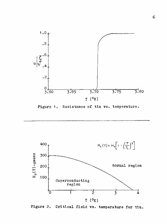
5temperature is shown in Fig. 1 Lowering the temperature below the critical temperature, in this case Tc = 3 .718°K, causes the electrical resistance to disappear. The sharpness of the transition from the normal state to the super state is largely determined by the homogeneity of the specimen,^ and the temperature width can vary from 0.3Tc to 10“^Tc.
As mentioned previously, superconductivity can be destroyed by the application of a sufficiently strong magnetic field. The transition temperature of all superconductors decreases as the applied magnetic field increases, as shown in Fig. 2 for tin.^ The relation between magnetic field and temperature may be approximated by the parabolic expression
HcfT) = H 0[l - (ffj (D
H0 is the magnetic field necessary to switch the specimen to the normal state at 0° Kelvin, and Hc(T) is the magnetic field necessary to switch the specimen to the normal state at temperature T. The parabola divides the quadrant into two regions: above and to the right, the metal is nomal; while below the parabola, it is in the superconducting state. The field at which the metal changes from super to normal is called the critical field, Hc. Self currents
(T)-
gaus
s
6
1
JlQO3.65 3.753-70
Figure 1. Resistance of tin vs. temperature.
normal region
m° 100 Superconductingregion
Figure 2. Critical field vs. temperature for tin.
exceeding a critical value will force a superconductor into the normal state. This effect was observed by Silsbee in 1916 as resulting from the magnetic field produced by the current. Subsequent experiments have shown the Silsbee hypothesis to be true only for pure unstrained elements. Compounds, alloys, and impure or strained elements do not obey the Silsbee Hypothesis.
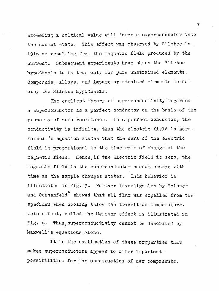
The earliest theory of superconductivity regarded a superconductor as a perfect conductor on the basis of the property of zero resistance. In a perfect conductor, the conductivity is infinite, thus the electric field is zero. Maxwell's equation states that the curl of the electric field is proportional to the time rate of change of the magnetic field. Hencesif the electric field is zero, the magnetic field in the superconductor cannot change with time as the sample changes states. This behavior is illustrated in Fig. 3» Further investigation by Meisner and Ochsenfeld^ showed that all flux was expelled from the specimen when cooling below the transition temperature.This effect, called the Meisner effect is illustrated in Fig. 4. Thus, superconductivity cannot be described by Maxwell's equations alone.
It is the combination of these properties that makes superconductors appear to offer important possibilities for the construction of new components.
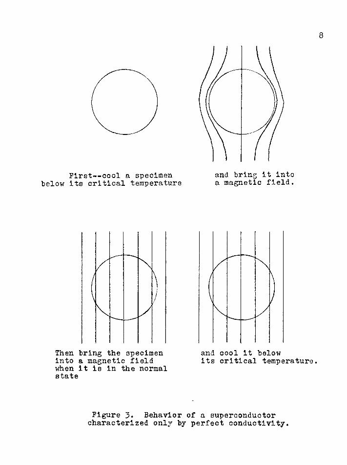
First--cool a specimen below its critical temperature
and bring it into a magnetic field.
Then bring the specimen into a magnetic field when it is in the normal state
and cool it below its critical temperatur
Figure 3. Behavior of a superconductor characterized only by perfect conductivity.
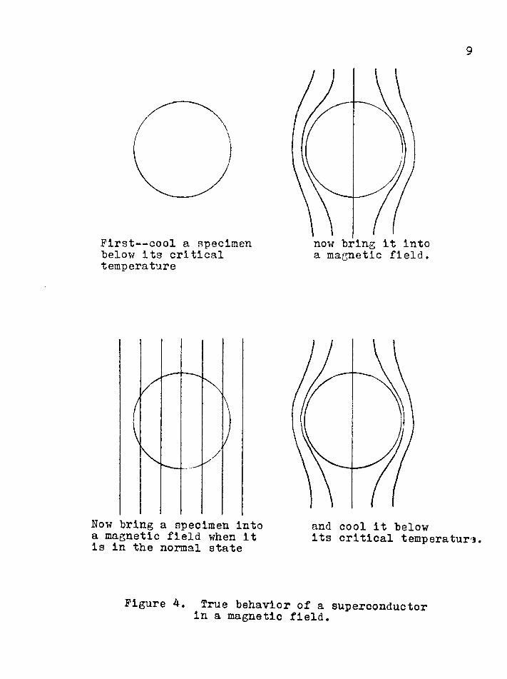
First— cool a specimen below Its critical temperature
Now bring a specimen into a magnetic field when it is in the normal state
9
now bring it intoa magnetic field.
and cool it belowits critical temperaturs.
Figure 4. True behavior of a superconductor in a magnetic field.
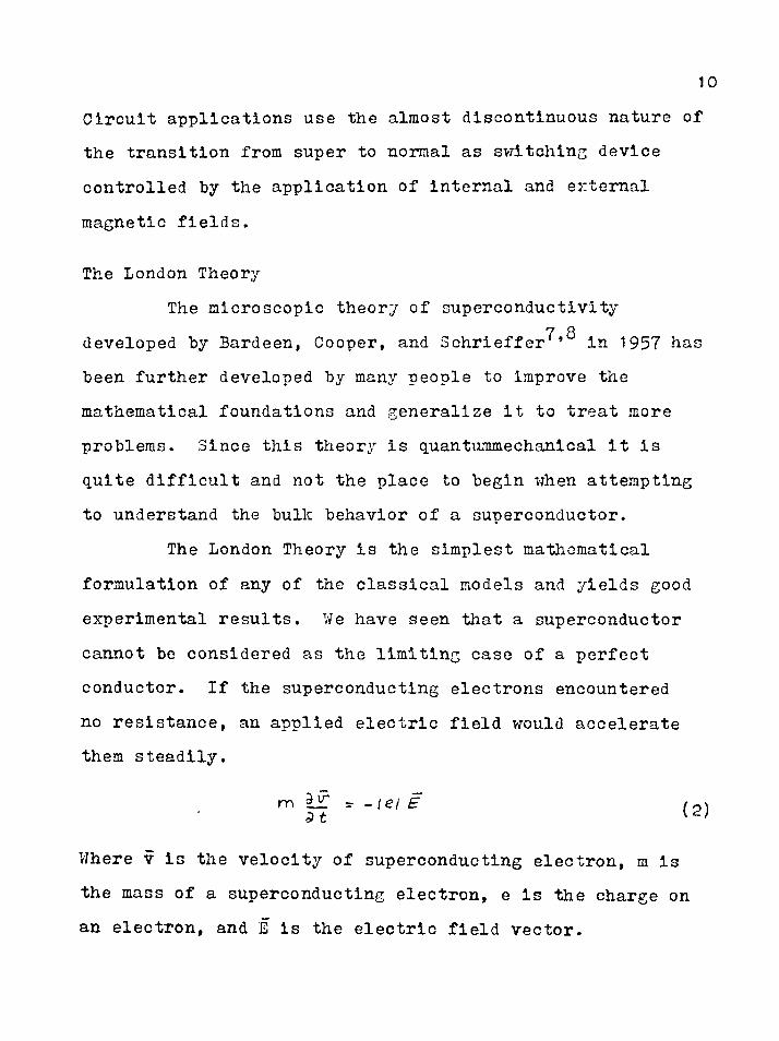
10Circuit applications use the almost discontinuous nature of the transition from super to normal as switching device controlled by the application of Internal and external magnetic fields.
The London TheoryThe microscopic theory of superconductivity
7 8developed by Bardeen, Cooper, and Schrieffer * in 1957 has been further developed by many people to improve the mathematical foundations and generalize it to treat more problems. Since this theory is quantummechanical it is quite difficult and not the place to begin when attempting to understand the bulk behavior of a superconductor.
The London Theory is the simplest mathematical formulation of any of the classical models and yields good experimental results. We have seen that a superconductor cannot be considered as the limiting case of a perfect conductor. If the superconducting electrons encountered no resistance, an applied electric field would accelerate them steadily.
m || = -,e,E (2)
Where v is the velocity of superconducting electron, m is the mass of a superconducting electron, e is the charge on an electron, and E is the electric field vector.
11
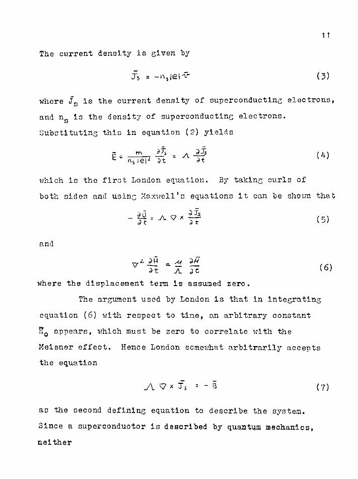
The current density is given by
= — k\|G|nr (3)
where Js is the current density of superconducting electrons, and n0 is the density of superconducting electrons. Substituting this in equation (2) yields
e - d b - i l ' ^ <4)
which is the first London equation. By taking curls of both sides and using Maxwell's equations it can be shown tha
- # (5)
and
V — - — — (6 )2. M __ x/It ~ X Jt
where the displacement term is assumed zero.The argument used by London is that in Integrating
equation (6 ) with respect to time, an arbitrary constant !T0 appears, which must be zero to correlate with the Meisner effect. Hence London somewhat arbitrarily accepts the equation
A V x = - B (7 )
as the second defining equation to describe the system.Since a superconductor is described by quantum mechanics, neither
cr
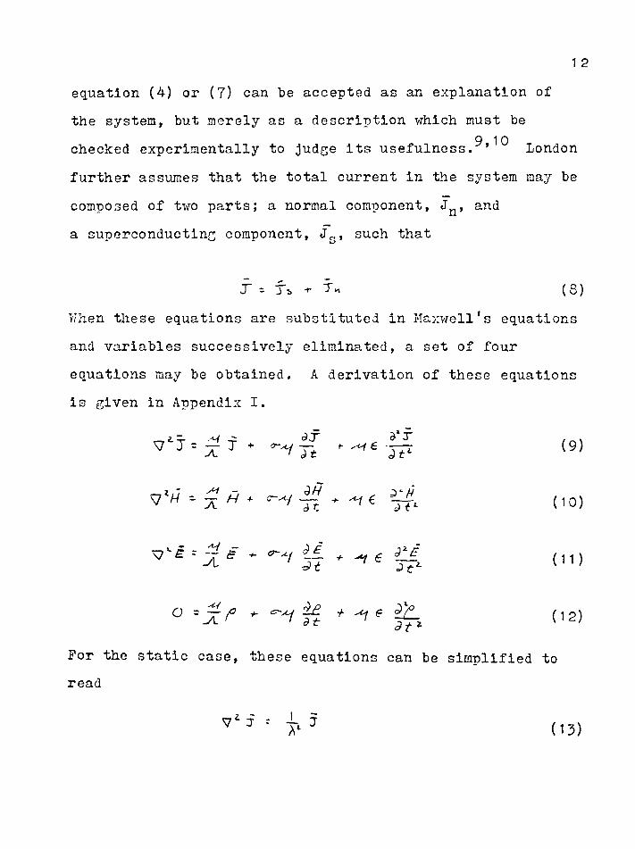
1 2equation (4) or (7) can be accepted as an explanation ofthe system, but merely as a description which must be
9 10checked experimentally to judge its usefulness. ' London further assumes that the total current in the system may becomposed of two parts; a normal component, J , anda superconducting component, Jg, such that
J~ =■ Tb ■*" ^ *1 (8 )When these equations are substituted in Maxwell’s equations and variables successively eliminated, a set of four equations may be obtained. A derivation of these equations is given in Appendix I.
V 2-J = J + ^ w 6 - ( 9 )
-- jl -jl + ^ (10)
-%£ * ^ Sf " ^ 6 (11)
r Z (12)
For the static case, these equations can be simplified to read
(13)
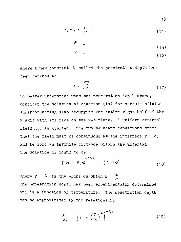
V*H -- H
13
(14)
E - o(15)(16)
Where a new constant X called the penetration depth has been defined as
x H atA " (17)
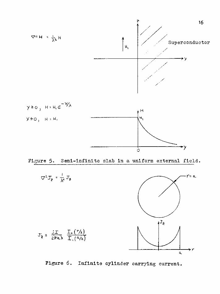
To better understand what the penetration depth means, consider the solution of equation (14) for a semi-infinite superconducting slab occupying the entire right half of the y axis with its face on the x-z plane. A uniform external field H1, is applied. The two boundary conditions state that the field must be continuous at the interface y = o, and be zero an infinite distance within the material.The solution is found to be
-v/aH<yi : e (y»o) (18)
Where y = \ Is the plane on which H = ijt The penetration depth has been experimentally determined and is a function of temperature. The penetration depth can be approximated by the relationship
- x - [' (,9>
where is the penetration depth at absolute zero.It is also instructive to note that the 3 field
zero everywhere in the superconductor, and the current i related only to the magnetic field.
III. METHODS OF SOLVING THE STATIC LONDON EQUATIONS
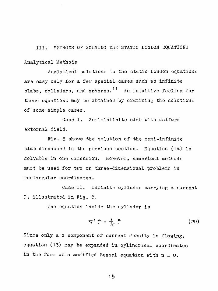
Analytical MethodsAnalytical solutions to the static London equations
are easy only for a few special cases such as infinite slabs, cylinders, and spheres. 11 An intuitive feeling for these equations may be obtained by examining the solutions of some simple cases.
Case I. Semi-infinite slab with uniform external field.
Fig. 5 shows the solution of the semi-infinite slab discussed in the previous section. Equation (14) is solvable in one dimension. However, numerical methods must be used for two or three-dimensional problems in rectangular coordinates.
Case II. Infinite cylinder carrying a current I, illustrated in Fig. 6 .
The equation inside the cylinder is
= (20)
Since only a z component of current density is flowing, equation (13) may be expanded in cylindrical coordinates in the form of a modified Bessel equation with n = 0 .
H - HSuperconductor
y * 0 } H - H( £~
V^O, H - M,
>
Figure 5. Semi-Infinite slab in a uniform external field.
X, % jx i.frA)
a.
Figure 6. Infinite cylinder carrying current
17
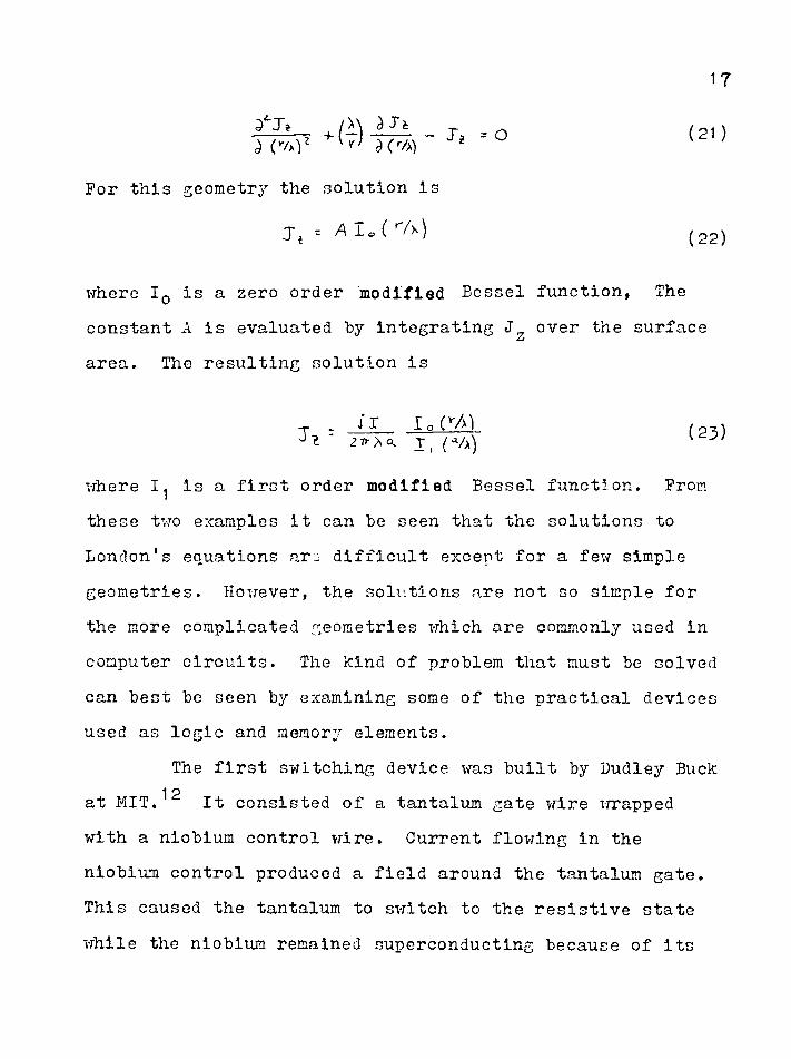
(21 )
For this geometry the solution Is
- A 1 o ( ) (22)
where I0 is a zero order modified Bessel function, The constant A is evaluated by integrating Jz over the surface area. The resulting solution is
where I is a first order modified Bessel function. From these two examples it can be seen that the solutions to London's equations arc difficult except for a few simple geometries. However, the solutions are not so simple for the more complicated geometries which are commonly used in computer circuits. The hind of problem that must be solved can best be seen by examining some of the practical devices used as logic and memory elements.
with a niobium control wire. Current flowing in the niobium control produced a field around the tantalum gate. This caused the tantalum to switch to the resistive state while the niobium remained superconducting because of its
T - 1 J In CVA) J * " I, (V a) (23)
The first switching device was built by Dudley Buck 1 2at MIT. It consisted of a tantalum gate wire wrapped
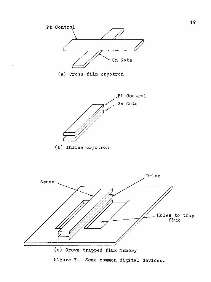
18higher critical field. This is the basis of all cryogeniclogic circuits. A memory cell may be constructed bytrapping a current in a loop of superconducting wire.Faster circuits made of evaporated thin films soon replacedthe bulkier wire wound ones. However, the principle ofoperation is identical. Figure 71^ 1 shows some commonlyused geometries.
Since resistance is first introduced in the gateat the point of maximum field Intensity, circuit designerscan learn much about the device by knowing the fieldpatterns that exist just prior to switching. In the devicesIllustrated in Fig. 7, the thicknesses of the insulating
olayers are about 10,000 A, and the thickness of the tin and lead range from 5,000 X to 10,000 A with line widths of the order of 20-60 microns. Hence it is difficult to measure any fields directly except possibly surface fields which may not yield any useful information.
Numerical MethodsThe only numerical solutions that have been done to
date are for two-dimensional geometries. The general procedure for solving a simple two-dimensional static problem will be illustrated.
Pb Control
Sn Cate
(a) Cross film cryotron
b ControlSn Gate
(b) Inline cryotron
DriveSense
Holes to trap flux
(c) Crowe trapped flux memoryFigure 7. Some common digital devices.
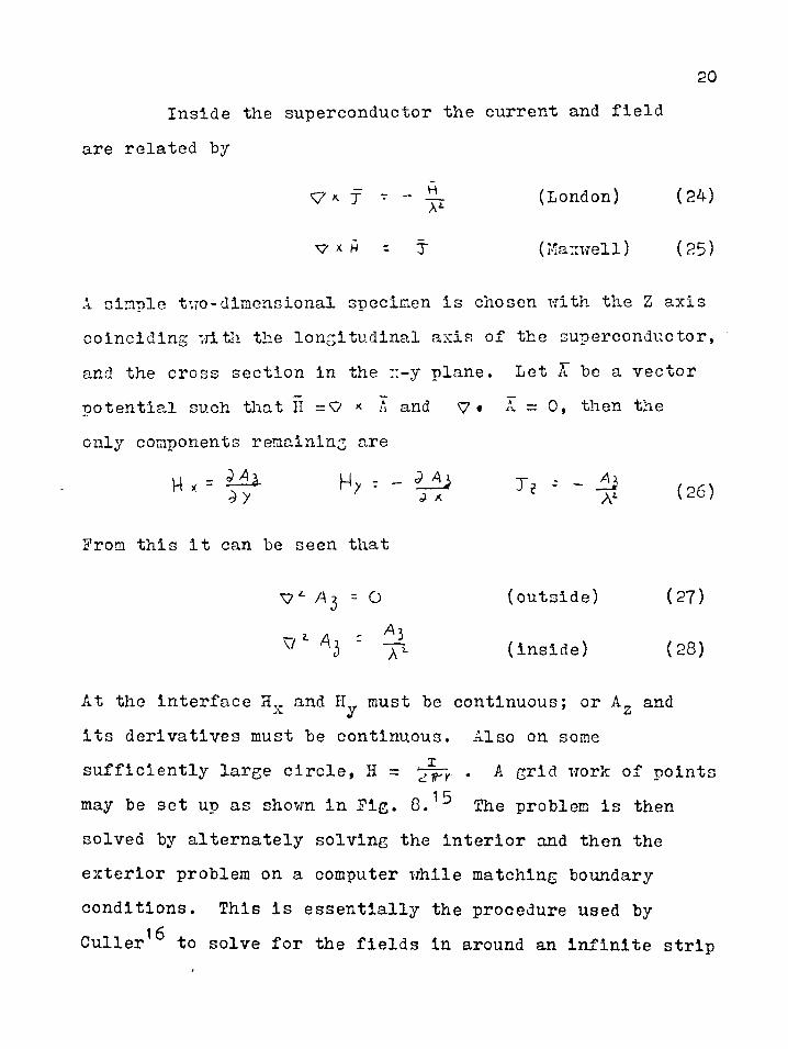
Inside the superconductor the current and field are related by
V * J - - (London) (24)
v x h - T (Maxwell) (25)
A simple two-dimensional specimen is chosen with the Z axis coinciding with the longitudinal axis of the superconductor, and the cross section in the ::-y plane. Let A be a vector potential such that H = V * A and V « A = 0, then the only components remaining are
M H>' " _ Ti "" ~ (26)
From this it can be seen that
Aj = O (outside) (2 7)
x/ ^3 ~p- (Inside) (2 8)
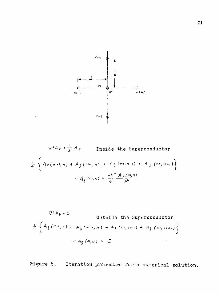
At the interface and H__ must be continuous; or A_ andy ^its derivatives must be continuous. Also on some sufficiently large circle, H = ^rr . A grid work of points may be set up as shown in Fig. 8 .1 The problem is then solved by alternately solving the interior and then the exterior problem on a computer while matching boundary conditions. This is essentially the procedure used by Culler1 to solve for the fields in around an infinite strip
21
o -hi (
h — <( — ,*
o n (
> 'I
-y
. '.. ...... ....IY)-I
h-| <
W nl-ht
v M * *-£ A £ Inside the Superconductor
A i (m +Ij h ) -f /A ( »>-!, h ) t- >4 ? Cm, n -,) + A (>n; n 4-# j'j
V 2/4e - O Outside the Superconductor^ ^ n ) A j n ) + A i (in, n~ t ) ■+ A ( tn) y; v / J
~ ' A ^ ( r > , n ) ~ C )
Figure 8 . Iteration procedure for a numerical solution.
22of rectangular cross section; except that the whole exterior region was transformed into a finite region hy use of a conformal map. Such computer solutions are time consuming and expensive. To date no three-dimensional problems of this type have been solved numerically.
Analog ModelsLarge scale superconductor.-Before constructing an
analog, the possibility of constructing a large scale superconductor should be investigated. Consider the crosssection of a typical superconducting tin gate 3 mills wide,
o o5,000 A thick and a penetration depth of 1,000 A. If thisis scaled up by a factor of 1,000, the physical dimensionswould be large enough to measure by conventional means.Also the thickness to penetration depth must be held
\ oconstant. A0 for tin is 520 A. Substituting this valuein equation (19) shows that T = 0.9994 Tc. At thistemperature the specimen breaks up into regions of normaland superconducting material called the mixed orintermediate state. London's equations of the puresuperconducting state are no longer valid. Thus, the fieldsaround a thin film circuit cannot be measured by directscaling.
Electrolytic tank m o d e l . The electrolytic tank analogy is derived from the similarity in form between the
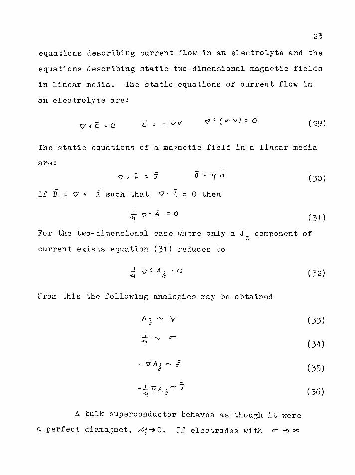
23equations describing current flow in an electrolyte and the equations describing static two-dimensional magnetic fields in linear media. The static equations of current flow in an electrolyte are:
V 1 ( <7- V ) r C (2 9 )
The static equations of a magnetic field in a linear media are:
s? x W - T 3 ’ H (3 Q)
If B = \7 * A such that v • I = o then^ v = 0 (31)
For the two-dimensional case where only a component ofcurrent exists equation (3 1) reduces to
4 1 ° (32)
From this the following analogies may be obtained
A 3 V (33)
(34)
(35)
(36)
A bulk superconductor behaves as though it werea perfect diamagnet, ^-*0. If electrodes with <r- <x>
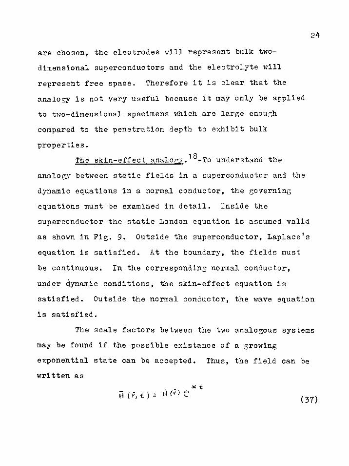
24are chosen, the electrodes will represent bulk two- dimensional superconductors and the electrolyte will represent free space. Therefore it Is clear that the analogy is not very useful because It may only be applied to two-dimensional specimens which are large enough compared to the penetration depth to exhibit bulk properties.
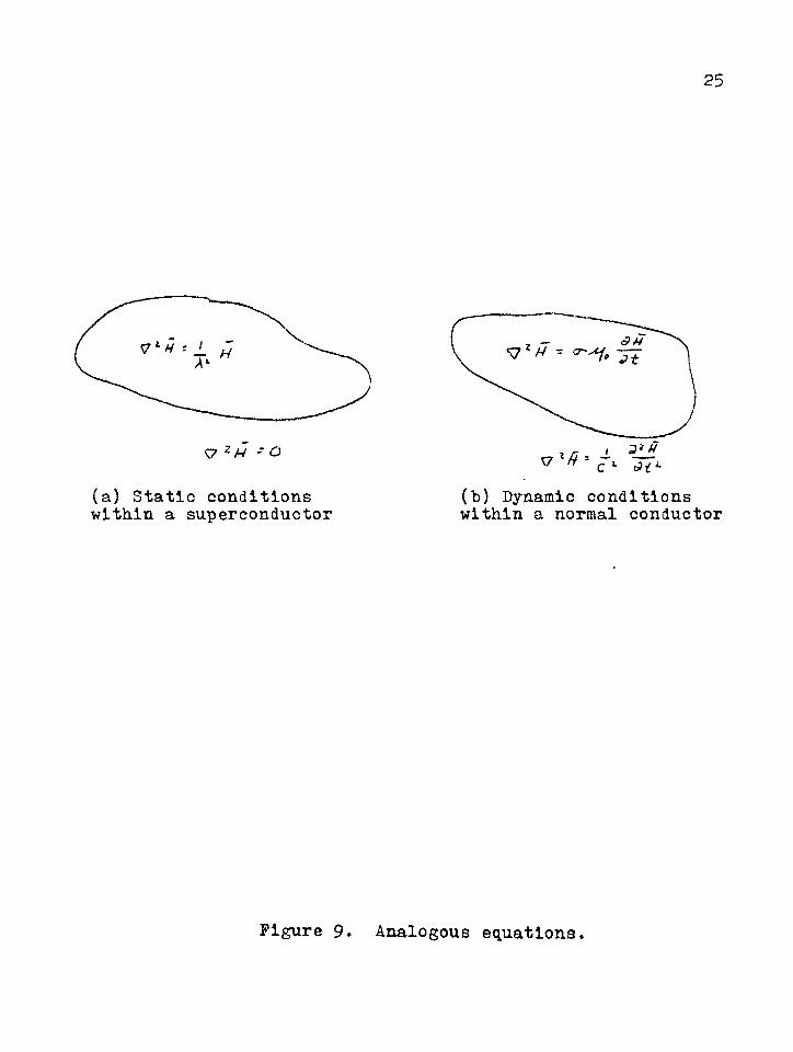
The skln-effect analogy.^-To understand the analogy between static fields in a superconductor and the dynamic equations in a normal conductor, the governing equations must be examined in detail. Inside the superconductor the static London equation is assumed valid as shown in Fig. 9. Outside the superconductor, Laplace’s equation is satisfied. At the boundary, the fields must be continuous. In the corresponding normal conductor, under dynamic conditions, the skln-effect equation is satisfied. Outside the normal conductor, the wave equation is satisfied.
The scale factors between the two analogous systems may be found if the possible exlstance of a growing exponential state can be accepted. Thus, the field can be written as
(37)
25
(a) Static conditions within a superconductor
2
(b) Dynamic conditions within a normal conductor
Figure 9. Analogous equations.
26If this form for the H field is substituted in theskln-effect equations, the result is found to be:
H (r ) - S’--Vo ot hi (r) (Inside) (38)
(Outside) (39)
The resulting equations are not quite the same as the static equations for the superconductor. However, if ^ is very small compared to czf the equations may be written as
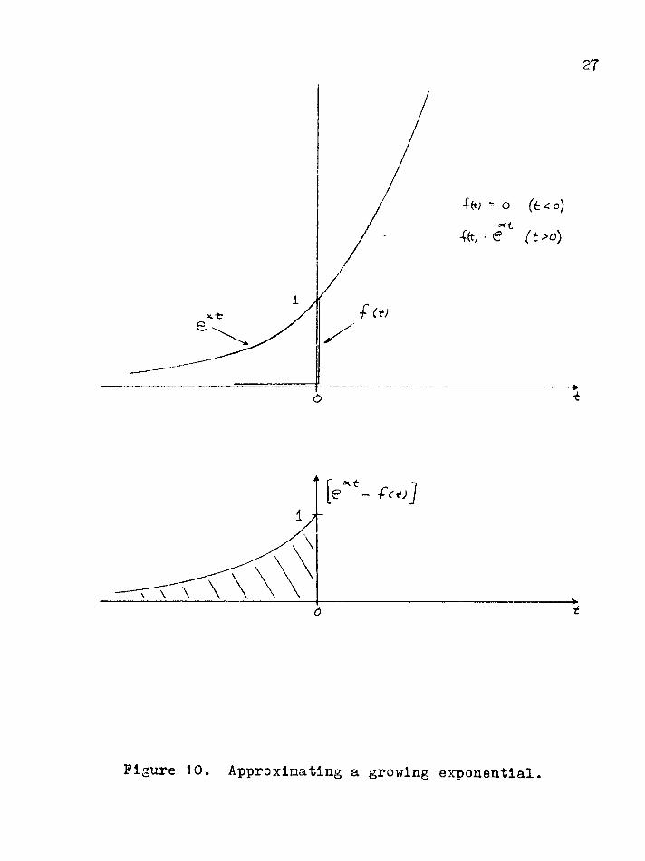
exponential state. It is, of course, Impossible to generate a perfect growing exponential. However, if the exponential is started a t = 0 as shown in Fig. 10, it will differ from the true exponential by the shaded amount shown.After several time constants, the value of f(t) will become so large that any transient due to the error will be small compared to the increasingly large signal. At this time a measurement of the field intensity could be made, and the excitation removed. After seven time constants f(t) is approximately 1100 times as large as its initial value.
(Inside) (40)
(Outside) (41)
Now reconsider th.3 postulation of a growing
27
t
1y[ e x < - f c - o ]
/ < X x
- r ^ X \ V( ---------- %
Figure 10. Approximating a growing exponential.
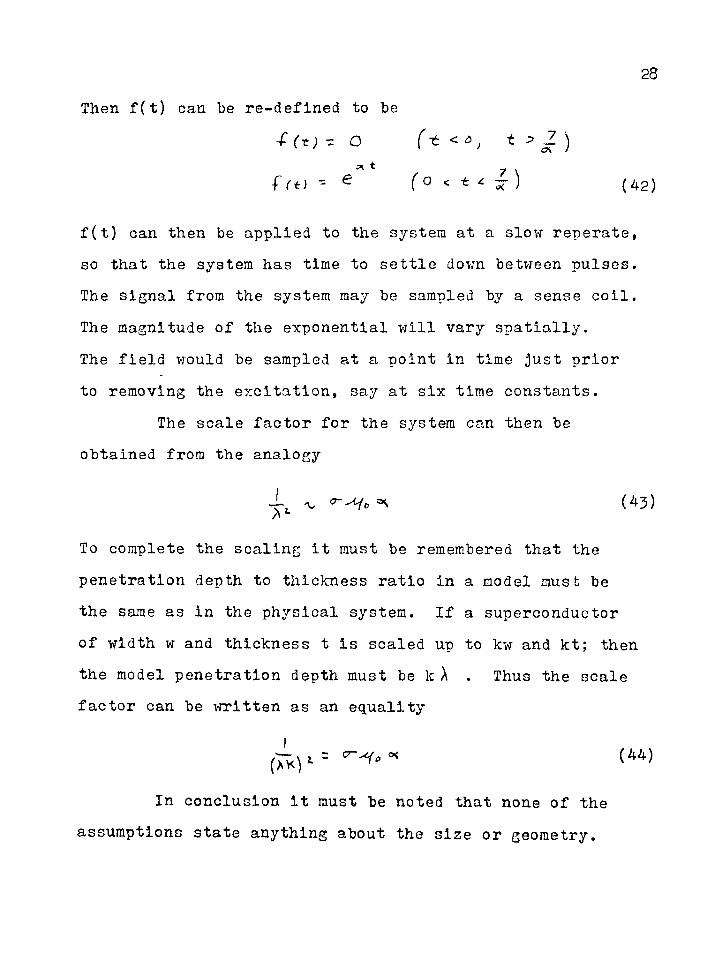
Then f(t) can be re-defined to be
(42)
f(t) can then be applied to the system at a slow reperate, so that the system has time to settle down between pulses. The signal from the system may be sampled by a sense coll. The magnitude of the exponential will vary spatially.The field would be sampled at a point in time just prior to removing the excitation, say at six time constants.
The scale factor for the system can then be obtained from the analogy
To complete the scaling it must be remembered that the penetration depth to thickness ratio in a model must be the same as in the physical system. If a superconductor of width w and thickness t is scaled up to kw and kt; then the model penetration depth must be k A . Thus the scale factor can be written as an equality
In conclusion it must be noted that none of the assumptions state anything about the size or geometry.
(43)
(44)
This model is good in three dimensions for a system of any thickness to penetration depth ratio. The only assumptions made were that (~) must be small, and an approximate growing exponential can be used to excite the system. This model is restricted to measuring only the external field distribution. The surface fields are usually of most interest since they can be used to predict when a specimen will change states. The accuracy to which the surface fields may be measured depends upon the size of the sense coil in relation to the sample.
IV. EXPERIMENTAL CONSIDERATIONS OF THESKIN EFFECT MODEL
Construetion of the Exponential Function GeneratorThere are several methods of generating a growing
exponential. The method selected depends to a great extent on the kind of equipment available. An exponential m a y be generated by use of a phototube and oscilloscope, or by a diode-resistor piecewlse-linear model.The piecewlse-linear model was chosen using Zener diodes and resistors to develop a non-linear impedance. A ramp voltage applied to the system produces a growing exponential of current. The accuracy of the piecewlse-linear model depends on the number of sections used. Since the signal will be differentiated by the sense coil and sense amplifiers, five sections were used to obtain good accuracy. The non-ideal Zener characteristics helped to improve the resulting wave form. With this type of driving signal, the growth rate of the exponential may be varied by changing the duration of the ramp input. Exponential pulses 7 time constants long were produced with durations of 5 milliseconds to 10CW second.
30
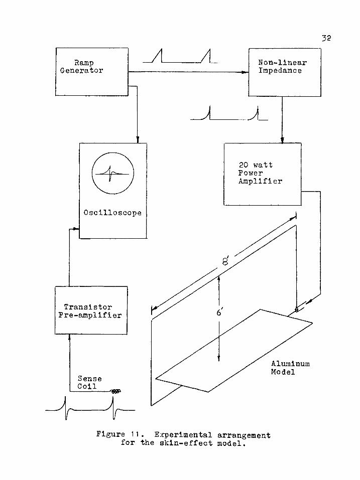
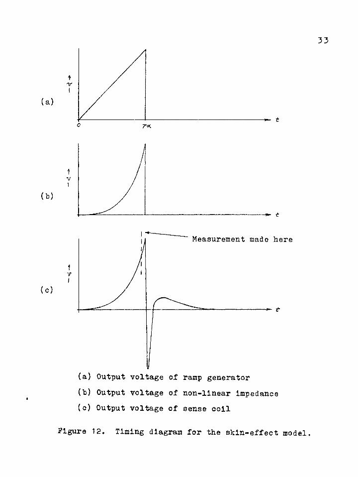
System ConsiderationsFig. 11 shows the completed experimental system.
Fig. 12 shows the time sequence of the system waveshapes.To check the accuracy of the system, data must be compared against some other source. If London's equations could be easily solved in some coordinate system such that the external fields of such a specimen would be a function of both geometry and penetration depth, data could be compared quite easily. Consider the cylinder carrying current in Case II. The field on the surface is \- - .The field is only a function of the radius. The simplest case that could be solved analytically where the external field is a function of both geometry and penetration depth would be an elliptic cylinder. The construction of an accurate model would be quite difficult.
An alternative approach was found in comparing data to an IBM 7090 computer solution of an infinite rectangular strip carrying current, which was performed byG. Culler at Space Technology Laboratory.1 Data were given in the form of plots of the vector potential Az.The most accurate field component that could be interpolated was the normal component. The field components may be obtained from the vector potential by use of equation (26).A model was built identical to one described, and data were compared to the computer solution. Very good agreement
32
Non-linearImpedance
RampGenerator
20 wattPowerAmplifier
Oscilloscope
TransistorPre-amplifier
AluminumModelSense
Coil
Figure 11. Experimental arrangement for the skin-effect model.
33
o
?V
t
Measurement made here
1v
(a) Output voltage of ramp generator(b) Output voltage of non-linear Impedance (o) Output voltage of sense coll
Figure 12. Timing diagram for the skin-effect model.

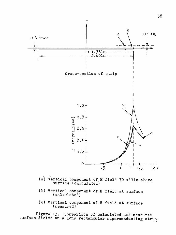
resulted when the size of the sense coil was taken into account as shown in Fig, 13- The computer solution of H one penetration depth (70 mills) above the surface is shown. This was the approximate location of the measuring coil on the model. The calculation of Hy at the surface shows the amount of error introduced because of the finite size of the coil. In this case the error was quite large. The measured field was 61% of the actual surface field. For thick specimens with sharp corners, the error will be the greatest at the corners, where the gradient of the field is the greatest. However, the coil still shows the approximate shape of the curve. It only rounds off the peaks because it is measuring the average over a finite area. This experiment provided two useful pieces of information.It checked the .accuracy of model., and it successfully showed the error in measuring with a sense coil of finite size which cannot be placed exactly at the surface.
The assumptions made can be checked easily with the probe. If any displacement current is flowing in the system, it will distort the field lines and be detectable. Since an infinite strip cannot be constructed, the field probe can also be used to map the surface currents on the finite strip. This will show that the fields in the center of a long strip are essentially those of an Infinite, strip.
35y
.08 Inch
-4 .331%■2 .66in
Cross-section of strip
0.8-
0 .2-
5 1 : . 1.5 2.0
(a) Vertical component of H field 70 mills abovesurface (calculated)
(b) Vertical component of H field at surface(calculated)
(c) Vertical component of H field at surface(measured)
Figure 13. Comparison of calculated and measured surface fields on a long rectangular superconducting strip.
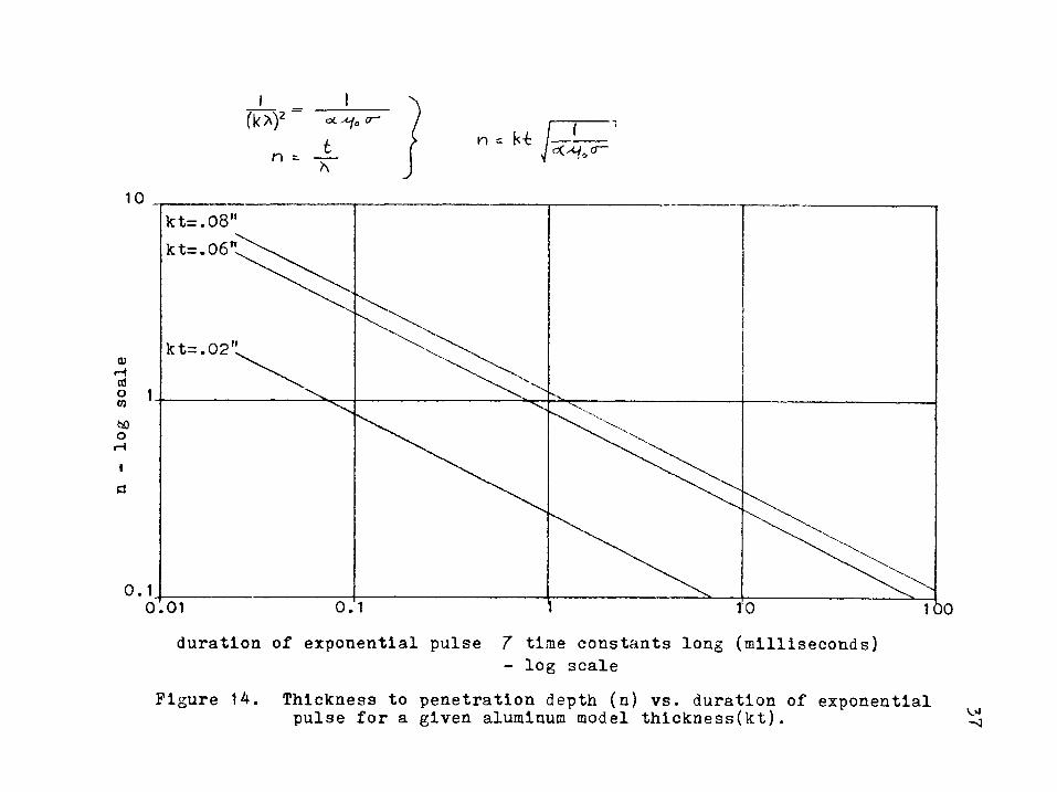
To aid in making measurements on the system, the equation
( t ^ " (45)
can be plotted as shown in Fig. 14.An approximate calculation of the power required to
drive a very thin aluminum strip 1 /j> meter wide and two meters long was made. In this approximate solution, the current distribution was assumed uniform. Since several approximations were made, the details have been shown in Appendix II. The results show that a 10-20 watt amplifier with a 4il output impedance is necessary to pick up 0.01 millivolts in a 150 turn pick up coil. Since the thicker strips do not have a uniform current distribution, this result is not valid in general. It was found that a 20 watt power amplifier provided adequate sensitivity for all measurements made.
log
scal
e(kX>2
n
Ot 0 C7-_6_A
n=k-& oC cr-
10
i
0.0.01 100
duration of exponential pulse 7 time constants long (milliseconds)- log scale
Figure 14. Thickness to penetration depth (n) vs. duration of exponentialpulse for a given aluminum model thlckness(kt). ^
V. AH ANALYSIS OP THE 3IDE-BY-SIDE CRYOTRON USING THE SKIN EPPEOT ANALOG
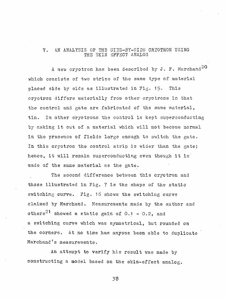
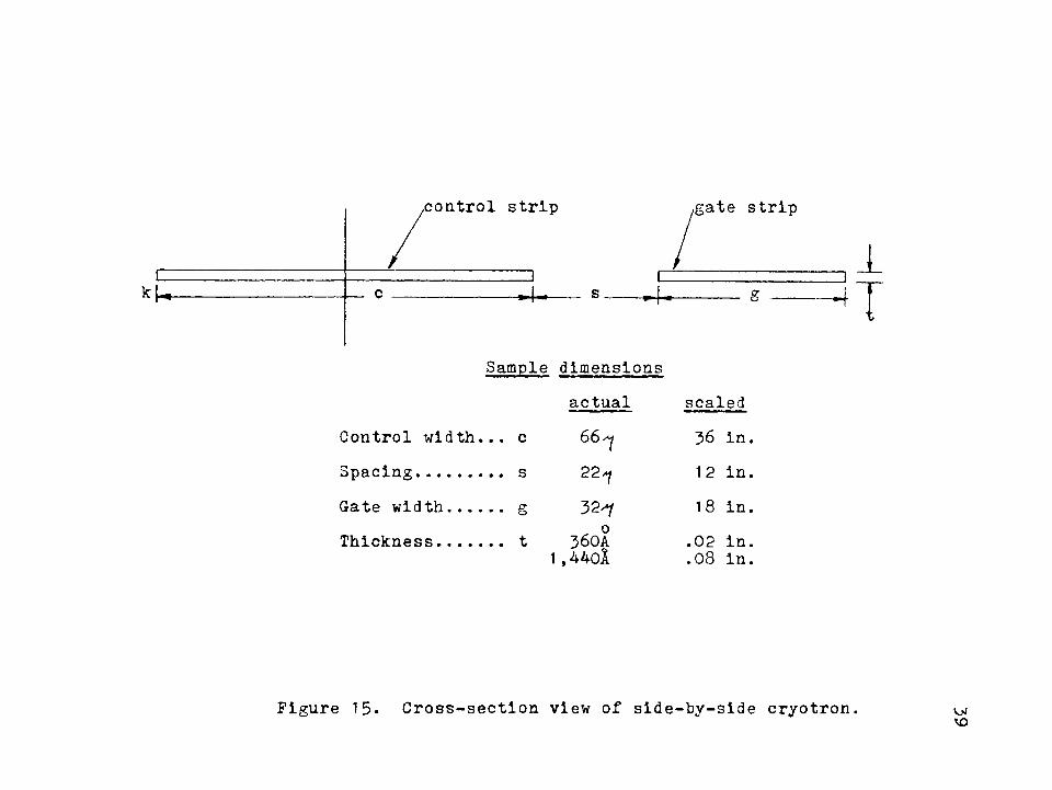
POA new cryotron has been described by J. P. Marchand which consists of two strips of the same type of material placed side by side as illustrated in Pig. 15• This cryotron differs materially from other cryotrons in that the control and gate are fabricated of the same material, tin. In other cryotrons the control is kept superconducting by making it out of a material which will not become normal in the presence of fields large enough to switch the gate.In this cryotron the control strip is wider than the gate; hence, it will remain superconducting even though it is made of the same material as the gate.
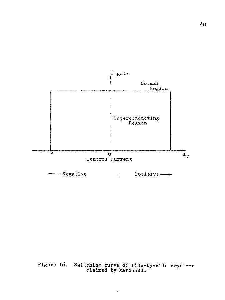
The second difference between this cryotron and those Illustrated in Pig. 7 is the shape of the static switching curve. Pig. 16 shows the switching curve claimed by Marchand. Measurements made by the author and others^ showed a static gain of 0.1 - 0.2, and a switching curve which was symmetrical, but rounded on the corners. At no time has anyone been able to duplicate Marchand’s measurements.
An attempt to verify his result was made by constructing a model based on the skin-effect analog.
3'8
^ y c o n t r o l strip
i:___ . z::.:.: : ik \~m----------------- C S
Sample dimensionsactual scaled
Control width... c 66 1 36 in.Spacing......... s 22^ 12 in.Gate width..... g 32-7 18 in.Thickness...... t „ o 360A
1,4401.02 in. .08 in.
,gate strip
Figure 15. Cross-section view of side-by-slde cryotron. vjvo
H h-4*
40
I gateNormal
Region
SuperconductingRegion
0 lcControl Current
Negative Positive
Figure 16. Switching curve of side-by-slde cryotronclaimed by Marchand.
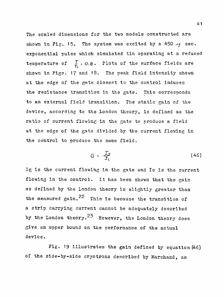
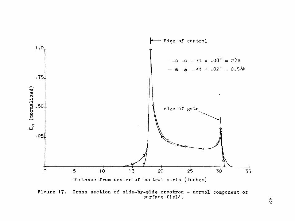
The scaled dimensions for the two models constructed are shown In Fig. 15. The system was excited by a 450 ^ sec. exponential pulse which simulated tin operating at a reduced temperature of — 5 o.Q . Plots of the surface fields areTcshown in Figs. 17 and 18. The peak field intensity shown at the edge of the gate closest to the control induces the resistance transition in the gate. This corresponds to an external field transition. The static gain of the device, according to the London theory, is defined as the ratio of current flowing in the gate to produce a field at the edge of the gate divided by the current flowing in the control to produce the same field.
G -- (46)-*C
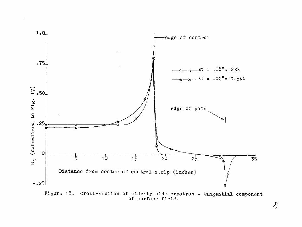
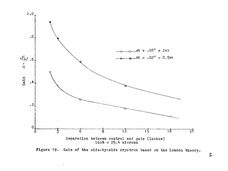
Ig is the current flowing in the gate and Ic is the current flowing in the control. It has been shown that the gain as defined by the London theory is slightly greater than the measured gain. This is because the transition of a strip carrying current cannot be adequately described by the London theory.However, the London theory does give an upper bound on the performance of the actual device.
Fig. 19 illustrates the gain defined by equation (46) of the side-by-slde cryotrons described by Marchand, as
(nor
mali
zed)
Edge of control
-G— o-.02
.75-
edge of gate
tim
5 10 15 20 25Distance from center of control strip (inches)
Figure 17- Cross section of side-by-side cryotron - normal component ofsurface field.
(normalized
to Fig. 17)
1 .CL.edge of control
—<5Sh
edge of gate
20
Distance from center of control strip (inches)
Figure 18. Cross-section of side-by-side cryotron - tangential componentof surface field.
Gain
1 .c>
.8
.6„ii<o
.4,_
00
.08
.02” = 0.5KA
t -4-—9 t 15 tSeparation between control and gate (inches)
inch = 25.4 micronsFigure 19. Gain of the side-by-slde cryotron based on the London theory.
£
a function of gate and control separation. A gain of sixowas claimed for the thinnest film (360 A) with a spacing
of twenty-two microns which corresponds to a model spacing of twelve Inches. The measured gain was 0.33. It was also claimed that the gain was constant for films up to 2000 8
thick. The measured gain for a film 1,440 8 thick was only 0.2. Thus the analog model shows a gain the same order of magnitude as measured by the author and others, but considerably different from Marchand. The computer solution has shown that considerable error results in measuring the peak fields at the edge of the gate. Since the gain is a ratio of two currents which produce the same field at the edge of the gate, the sense coil does not affect the accuracy.
71. CONCLUSIONS
ConclusionsIt has been demonstrated that analog models provide
a convenient method for solving the static London equations of superconductivity. In particular the skin-effeet analogy9 which is based on an analogy between the static London equations and the dynamic skin-effect equations under a growing exponential excitation* has been shown to be a flexible method of solving the boundary value problems of interest.
This thesis has contributed to the understanding of the skln-effect analogy in the following ways:
1. The accuracy of the skln-effect model was determined by comparing data taken on a long rectangular strip to data obtained from a computer solution of an infinite superconducting strip of rectangular cross-section. Previous workers made no attempt to correlate data taken with the skin-effect model to any analytical or numerical solutions.
2 . The effect of large field gradient on the accuracy of the sense coil signal was noted. The computer solutions mentioned above provided a convenient means to determine the fields near the corners of a long rectangular
47strip. As above, previous workers assumed the finite size of the coil caused sharp peaks to be rounded off, but did not determine the amount of inaccuracy introduced.
The skin-effect model has also been used to analyze a geometry of recent interest, the side-by-side cryotron.The gain of the side-by-side cryotron as defined by the London theory has been measured using the skin«>effect model. Previous workers have shown that the London theory does not correctly describe the gain of a cryotron, but yields a gain slightly higher than the actual device. Data taken on an actual thin film side-by-side cryotron by the author and co-workers showed the same trend.
Suggestions for Further StudyThe skin-effect analogy can be used to solve for
the surface and external magnetic fields. An interesting problem results when the.solution of the interior problem is desired. A digital computer solution for a two-dimensional superconductor using an iterative procedure converges slowly because the exterior region is unbounded„ If the surface data from the skin-effect analog were used as boundary values, the numerical solution could be reduced from a time consuming open boundary problem to a shorter closed boundary problem.It is also possible that a combination of these two methods could be used to solve three-dimensional problems.
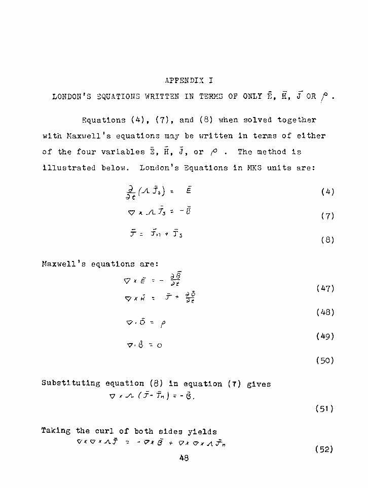
APPENDIX ILONDON'S EQUATIONS WRITTEN IN TERMS OF ONLY E, H, f OR f .
Equations (4), (7), and (8) when solved together with Maxwell's equations may be written in terms of either of the four variables S, H, J, or . The method is illustrated below. London's Equations in MKS units are:
^ fW J5) -- £ (4)
V x -A- - - 6
T - fn i f 5
Maxwell's equations are:
V'O -
v- 6 - o
Substituting equation (8 ) in equation (7) gives V * -/V f J- TV, J = - Q ,
Taking the curl of both sides yieldsV < V * A >7 - ' <7 X B ■+ \7 A <7 JC A J1*
48
(7)
(8)
(47)
(48)
(49)
(50)
(51)
(52)
(53)
(54)
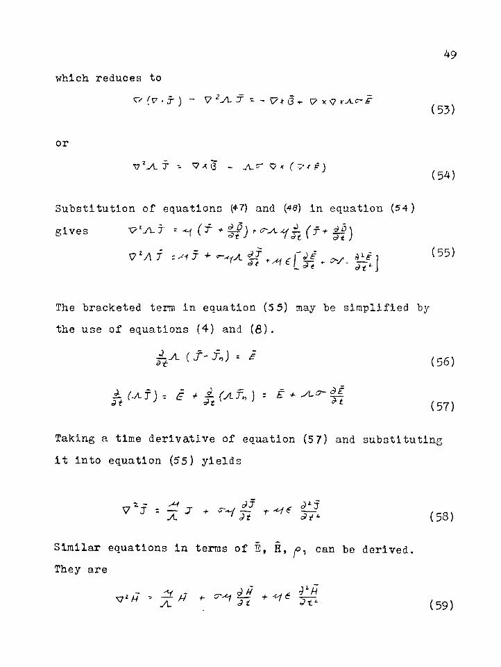
which reduces toV/ fv ' j- ) - V zj\- T - - v- (3 f 7 x <7 xJLCT-jr
or\72A.T - V/ g - VL^^/xfv'rFj
Substitution of equations (47) and (49) in equation (54) gives ^ (r +
V M T ^ 7 + r-^x |7 f , v. |L< j ( 55)
The bracketed term in equation (5 5) may be simplified by the use of equations (4) and (8 ).
^ V L (f- f*) * £ (56)
A (.ATJ -. £ + £-t (JIT* ) - B *■ VU5-(57)
Taking a time derivative of equation (5 7) and substituting it into equation (55) yields
Similar equations in terras of 3, H, can be derived. They are
50
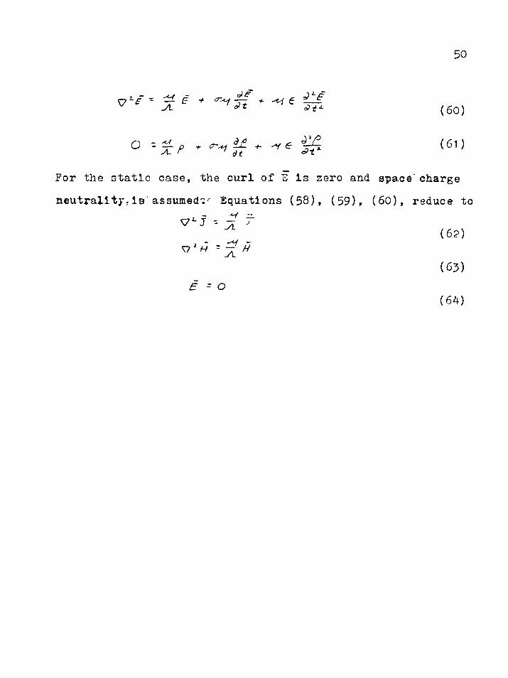
v'i- % Z + <»ig + ~ < e £ I (6o)
O ~ ~7r p + +- 'V 6 (61)vt ' ' J t < * t
For the static case, the curl of E Is zero and space'charge neutrality, is' assumed'; Equations (58), (59), (6 0), reduce to
n'H(6 3 )
E - O(64)
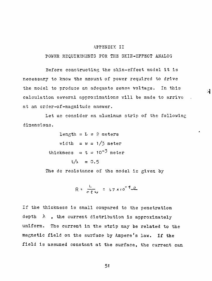
APPENDIX IIPOWER REQUIREMENTS FOR THE SKIN-EFFECT ANALOG
Before constructing the skin-effect model it is necessary to know the amount of power required to drive the model to produce an adequate sense voltage. In this calculation several approximations will be made to arrive at an order-of-magnitude answer.
Let us consider an aluminum strip of the following dimensions.
length = L = 2 meters width = w = l/ 3 meter
thickness = t = 10"" metert A = 0.5
The dc resistance of the model is given by
R - ^ = 17 * 10" *-4.
If the thickness is small compared to the penetration depth > , the current distribution is approximatelyuniform. The current in the strip may be related to the magnetic field on the surface by Ampere's law. If the field is assumed constant at the surface, the current can
A
51
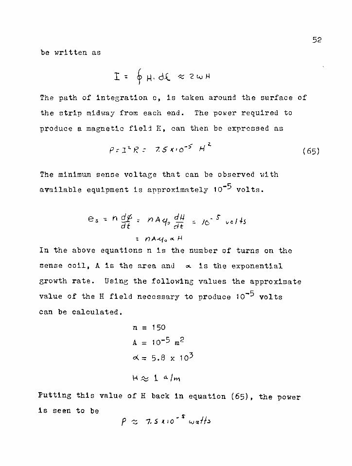
52be written as
I - ? uj H
The path of integration c, is taken around the surface of the strip midway from each end. The power required to produce a magnetic field H, can then be expressed as
r 2 7. 5 X'O'* M (65)
The minimum sense voltage that can be observed with available equipment is approximately 10“ volts.
e* -- z dji = /6- i- vc,^
Z /OA-C/o ocIn the above equations n is the number of turns on the sense coil, A is the area and <*. Is the exponential growth rate. Using the following values the approximate value of the H field necessary to produce 10~^ volts can be calculated.
n = 1 50 A = 10-5= 5.8 x 10³
H 1 a I m
Putting this value of H back in equation (6 5), the power is seen to be
P ~ 7, S A I0~ ujcffh

53Since a current of approximately 1 amp is required, a power amplifier was chosen. A great amount of power is lost in matching to an amplifier with 4 XL output impedance.The power supplied by the amplifier must then be about 17 watts. A 20 watt amplifier provided satisfactory sensitivity for all measurements made.
REFERENCES
H. E. Kronlck, "Magnetic Field Plotter for Superconducting Films„ IBM Journal of Research and Development8 Vol. 2, Ho. July 1958, p. 252.
2D. Schoenberg, Superconductivity, The University Press, Cambridge, England, 1 <260, p. 1.
R. Delano, Jr., "Edge Effects In Superconducting Films," Symposium on Superconductive Techniques for Computing Systems, Office of Naval Research Symposium Report ACR-=50, Washington, D. C., May 17-19, I960, p. 327.
A. Brenneman, "Properties of Thin Film Cryotrons," Symposium on Superconductive Techniques for Computing Systems, Office of Naval Research Symposium Report ACR-50, Washington, D. C., May 17-19, I960 p. 327.
D, Schoenberg, Superconductivity, The University Press, Cambridge, EnglanT7l^50g p. H
F. London, Superfluids, Vol. 1, Dover Publications, Inc., Hew York, H. 77% i960', pT 3.
J. Bardeen, L. H. Cooper, and J. R, Schrieffer,"The Theory of Superconductivity," The Physical Review,Vol. 108, 1957, p. 1175.
^J. Bardeen, "Review of the Present Status of the Theory of Superconductivity," IBM Journal of Research and Development, Vol. 6 , Ho. 1, January 1962, p. 3.
9F. London, Superfluids. Vol. 1., Dover Publications, Inc., Hew York, H. Y., I9 6 0, p. 5 3.1 0D. Schoenberg, Superconductivity. University Press, Cambridge, England, i9 6 0, p. 192.11 Ibid. p. 233.1 2D, A. Buck, "The Cryotron - A Superconductive
Computer Element," Proceedings of the IRE, Vol. 44, April, 1956, p. 482.
54
551 "J>"u, if. Bremmer, Superconductive Devices, McGraw-Hill,
lew York, 1962, p. 57.14Illd, p, 130. . M. Morse, H. Feshbach, Methods of Theoretical
Physics, Part 1, McGraw-Hill, Hew York, 1953$ p. 706.^G. J. duller, "Current and Magnetic Field
Distribution for an Infinitely Long Superconductor of Rectangular Oross-Sectlon," Report Ho. 9844-0011-RU-000,Space Technology Laboratory, Los Angeles, California,March, I9 6 0, p. 2.
1 . A. Kurtz, IBM Research Laboratory, Poughkeepsie,H. Y., Private Communication.
®H. H. Meyers, "An Analog Solution for the Static London Equations of Superconductivity, 11 Symposium on Superconductive Techniques for Computing Systems, Office of Haval Research Symposium Report ACR-50, Washington, D. 0., May 17-19, I960, p. 331.
19G. J. Culler, "Current and Magnetic Field Distribution for an Infinitely Long Superconductor of Rectangular Cross-Section," Report HO. 9844-0011-RU-000,Space Technology Laboratory, Los Angeles, California,March, 1960, p. 21.
F. Marchand, "Properties of A Hew Type of Parallel Cryotron, 11 Philips Research Laboratories,Eindhoven - Netherlands; Abstract of a talk given at The London Low Temperature Conference, London, England, September, 1962.
21A. Brenneman, IBM Thomas J. Watson Research Center, Yorktown Heights, Hew York, Private Communication.'
22A. Brenneman, "Properties of Thin Film Cryotrons, 11 Symposium on Superconductive Techniques for Computing Systems, Office of Naval Research Symposium Report ACR-5 0, Washington, D. 0., May 17-19, I960, p. 366.
23Ibid, p. 372.