Mathematical Medicine and Biology(2008)25, 187−214doi:10.1093/imammb/dqn013Advance Access publication on July 14, 2008

An overset grid method for the study of reflex tearing

K. L. M AKI , R. J. BRAUN† AND T. A. DRISCOLL

Department of Mathematical Sciences, University of Delaware, Newark, DE 19711, USA

AND

P. E. KING-SMITH

College of Optometry, The Ohio State University, Columbus, OH 43218, USA

[Received on 19 February 2008; revised on 29 May 2008; accepted on 30 May 2008]

We present an overset grid method to simulate the evolution of human tear film thickness subject toreflex tearing. The free-surface evolution is governed by a single fourth-order non-linear equation de-rived from lubrication theory with specified film thickness and volume flux at each end. The model arisesfrom considering the limiting case where the surfactant is strongly affecting the surface tension. In numer-ical simulations, the overset grid is composed of fine boundary grids near the upper and lower eyelids tocapture localized capillary thinning referred to as ‘black lines’ and a Cartesian grid covers the remainingdomain. Numerical studies are performed on a non-linear test problem to confirm the accuracy and con-vergence of the scheme. The computations on the tear film model show qualitative agreement within vivotear film thickness measurements. Furthermore, the role of the black lines in the presence of tear supplyfrom the lid margins, reflex tearing, was found to be more subtle than a barrier to tear fluid flow betweenthe anterior of the eye and the meniscus at the lid margin. During reflex tearing, tears may flow through theregion normally containing the black line and drift down over the cornea under the influence of gravity.

Keywords: tear film; reflex tearing; black line; overset grid; lubrication theory.

1. Introduction

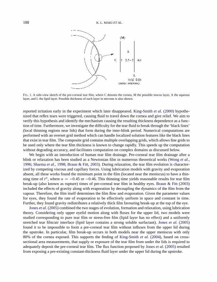
The human tear film is typically thought of as a multilayer structure encapsulated in a time-dependentregion playing a vital role in the health and function of the eye. Figure1 displays the multilayer structurewith the first layer (above the cornea) being a potential mucus layer made of gel-forming mucins whoseexistence is still debated. Next is the aqueous layer consisting primarily of water and commonly thoughtof as tears. Finally, the lipid layer, which has an outer non-polar layer with polar surfactants at theaqueous/lipid interface, decreases the surface tension and retards water evaporation.

The time-dependent domain moves in accordance with the blink cycle, comprised of two subsequentparts in this study: the upstroke or opening of the lids and the inter-blink where the lids are kept open.Findings on the phenomenon of reflex tearing indicate that one mechanism triggering the onset of tearingis activation of the sensory nerves in the cornea (Maitchouket al., 2000). Corneal dehydration, coolingor trauma could be potential triggers, as is the watering of one’s eyes from cutting an onion.

In this work, we study the formation and relaxation of the aqueous layer including the phenomenonof reflex tearing.King-Smithet al.(2000) published anin vivo tear film thickness measurement taken atthe centre of the cornea in a subject who kept his eyes open for a remarkable 360 s; this ‘six-minute man’

†Email: braun@math.udel.edu

c© The author 2008. Published by Oxford University Press on behalf of the Institute of Mathematics and its Applications. All rights reserved.

188 K. L. MAKI ET AL.

FIG. 1. A side-view sketch of the pre-corneal tear film, where C denotes the cornea, M the possible mucus layer, A the aqueouslayer, and L the lipid layer. Possible thickness of each layer in microns is also shown.

reported irritation early in the experiment which later disappeared.King-Smith et al. (2000) hypothe-sized that reflex tears were triggered, causing fluid to travel down the cornea and give relief. We aim toverify this hypothesis and identify the mechanism causing the resulting thickness dependence as a func-tion of time. Furthermore, we investigate the difficulty for the tear fluid to break through the ‘black lines’(local thinning regions near lids) that form during the inter-blink period. Numerical computations areperformed with an overset grid method which can handle localized solution features like the black linesthat exist in tear film. The composite grid contains multiple overlapping grids, which allows fine grids tobe used only where the tear film thickness is known to change rapidly. This speeds up the computationwithout degrading accuracy, and facilitates computation on complex domains as discussed below.

We begin with an introduction of human tear film drainage. Pre-corneal tear film drainage after ablink or relaxation has been studied as a Newtonian film in numerous theoretical works (Wong et al.,1996; Sharmaet al., 1998; Braun & Fitt, 2003). During relaxation, the tear film evolution is character-ized by competing viscous and capillary forces. Using lubrication models with gravity and evaporationabsent, all these works found the minimum point in the film (located near the meniscus) to have a thin-ning time oftα, whereα = −0.45 or−0.46. This thinning time yields reasonable results for tear filmbreak-up (also known as rupture) times of pre-corneal tear film in healthy eyes.Braun & Fitt (2003)included the effects of gravity along with evaporation by decoupling the dynamics of the film from thevapour. Therefore, the film itself determines the film flow and evaporation. Given the parameter valuesfor eyes, they found the rate of evaporation to be effectively uniform in space and constant in time.Further, they found gravity redistributes a relatively thick film favouring break-up at the top of the eye.

Joneset al.(2005) combined the two stages of evolution, formation and relaxation, using lubricationtheory. Considering only upper eyelid motion along with fluxes for the upper lid, two models werestudied corresponding to pure tear film or stress-free film (lipid layer has no effect) and a uniformlystretched tear film/air interface (lipid layer contains a strong soluble surfactant).Joneset al. (2005)found it to be impossible to form a pre-corneal tear film without influxes from the upper lid duringthe upstroke. In particular, film break-up occurs in both models near the upper meniscus with only80% of the cornea exposed. This supports the finding ofKing-Smith et al. (2004), based on cross-sectional area measurements, that supply or exposure of the tear film from under the lids is required toadequately deposit the pre-corneal tear film. The flux function proposed byJoneset al. (2005) resultedfrom exposing a pre-existing constant-thickness fluid layer under the upper lid during the upstroke.

REFLEX TEARING 189

Building upon the formation and relaxation models ofJoneset al. (2005), Heryudonoet al. (2008)studied the two models described above over multiple blink cycles and partial or half blinks withrealistic lid motion functions fit from observed lid motion data. They developed generalized flux bound-ary conditions, including supply from the lacrimal gland and drainage through the puncta. In their nu-merical study, better comparisons toin vivo measured partial blink data were found when using theuniform stretching limit model coupled with the generalized flux functions.

In this paper, we model the formation and relaxation of the tear film with the uniform stretching limitmodel. Since we wish to simulate the relaxation or the inter-blink period for an extended period of timewhen compared to the typical blink cycle, the effects of evaporation and gravity will be of importanceand hence included. The end fluxes are modified functions previously used byHeryudonoet al. (2008)with modification to incorporate reflex tearing.

The lubrication-type problem can be characterized as being of the formht + (hnhxxx)x = 0; fluidmechanics problems haven = 3, typically, but may have additional terms and equations. The maindifficulties for numerical solution appear to be related to having these terms present, generally speaking.Numerical methods in previous one-spatial-dimension studies for problems closely related to this formhave used a method of lines approach with differences in choice of spatial approximations and timeintegration. Some combinations include finite-difference spatial approximations on uniformly spacedgrids in space with BDF-type solvers in time (e.g.Jensen & Grotberg, 1993; Braun & Fitt, 2003),the package PDECOL (Madsen & Sincovec, 1979) which implements finite-element discretization inspace (Yeo et al., 2003), spectral spatial approximations on a fixed domain with BDF-type solvers intime (Haley & Miksis, 1991), a dynamically adaptive finite-difference method specifically designed tominimize round-off error with a two-level time-stepping scheme (Bertozziet al., 1994) and a positivity-preserving spatial approximation based on a modified partial differential equation (PDE) that uses finitedifferences and requires much less resolution than the original PDE (Zhornitskaya & Bertozzi, 2000).A mapped spectral discretization coupled with BDF-type solvers in time was used byHeryudonoet al.(2008) for a closely related problem with moving ends, specifically the tear film evolution over repeatedblink cycles.

The calculations were carried out in this paper with an overset grid method. In an overset gridmethod, a PDE is discretized and solved on a composite or overlapping grid developed to handle com-plex geometries or localized solution features. A composite grid contains multiple structured componentgrids, each being topologically rectangular, with interpolation information used for communication be-tween the separate grids. Composite grids have a number of advantages including the following: simplegrid generation since each component grid is built separately, easy addition or subtraction of bodies orfeatures and the ability to locally adapt the grid. These appealing features along with the handling ofcomplex geometries will be of importance when considering tear film flow on the entire anterior sur-face of the eye. They were first used byVolkov (1966, 1968) to solve Poisson’s equation on regionswith corners (finite domains with piecewise smooth boundaries) and in principle they utilize the samedifferencing techniques needed on a Cartesian grid with slight generalization. Code developments incomposite grid generation include CMPGRD tools byChesshire & Henshaw(1990), which later be-came the OVERTURE framework (Henshaw, 2002); an approach called Chimera grids by Steger andassociates was developed independently at National Aeronautics and Space Administration (NASA)(Steger & Benek, 1987). Composite grids have been used successfully for numerical simulations in-cluding non-Newtonian Hele–Shaw flow (Fast & Shelley, 2004). Our discretization is finite differencebased and again leads us towards our destination of simulations on a 2D eye-shaped domain. Previouswork in two dimensions for lubrication-type problems has often used alternating direction implicit(ADI) methods for spatial approximations on rectangular domains (e.g.Witelski & Bowen, 2003, and

190 K. L. MAKI ET AL.

references therein) but others have used positivity-preserving schemes (Diez & Kondic, 2002) and spec-tral methods (Ye & Chang, 1999) for spatial approximations. For finding the thin-film flow given byour particular equations on a moving eye-shaped domain, we believe that the overset grid methods asimplemented in OVERTURE will be quite effective, and so we start towards that goal by using oversetgrids in this paper.

After formulating the tear film problem in Section2, we explore the consequences of three differentdiscretizations of a simplified test problem in Section3 settling on the most accurate and robust methodof the three. Relevant grid parameters for the numerical method are determined from the test problemand subsequently used on the tear film problem. Results for the tear film model are presented in Section4with conclusions about the numerical method and reflex tearing.

2. Formulation

First, we present the model for the blink cycle of the human tear film derived from lubrication theory.

2.1 Tear film model

A sketch of the tear film model is shown in Fig.2. Primed variables indicate dimensional quantities. Thecorneal surface is modelled as a flat wall (y′ = 0) due to the tear film thickness being so much smallerthan the radius of curvature of the eye surface (seeBerger & Corrsin, 1974). Gravity acts in the positivex′-direction along the wall with the free-surface depthy′ = h′(x′, t ′) being measured perpendicular tothe wall. The velocity components of the film are denoted by(u′, v′). The lower lid is fixed atx′ = L ′,while the upper lid moves according tox′ = X′(t ′) with the eye fully open when the upper lid locationis x′ = −L ′.

We begin with the Navier–Stokes equation and scale by the half width of the palpebral fissure(corneal surface between the two lids),L ′ = 5 mm, in thex′-direction; the characteristic tear film thick-ness away from the lidsd′ = 5 μm applied in they′-direction; the velocity scale,Um = 10–30 cm/s,whereUm is a representative maximum blink closing speed (Doane, 1980; Berke & Mueller, 1998),applied along the tear film; the timescale for real blink speedL ′/Um and the viscous scaleμUm/(d′ε)applied to the pressurep. The small parameter for lubrication theory is the ratio of the length scales,ε = d′/L ′, approximately 10−3. Other relevant quantities needed in the derivation are the surface ten-sionσ0 = 45 mN/m (where subscript 0 denotes evaluation at the reference point corresponding to theeye fully open with the lowest average surface concentration of surfactant), the densityρ = 103 kg/m3,the viscosityμ = 10−3 Pa s and the gravitational accelerationg = 9.81 m/s2.

After non-dimensionalization, the leading-order terms in the mass conservation equation and mo-mentum conservation equation in thex- and y-directions, respectively, govern the following parallelflow on 06 y 6 h(x, t):

ux + vy = 0, uyy − px + G = 0 and py = 0. (1)

Here,G = ρg(d′)2

μUmis the Stokes number and under typical blink conditions,G ≈ 2.5 × 10−3. At the

impermeable wall, we have the Navier slip condition (to imitate the effects of the mucus and microplicaeat the corneal surface) and impermeability:

u = βuy and v = 0 at y = 0, (2)

whereβ = L′

s/d′ andL′

s is the slip length. Using the estimate inBraun & Fitt (2003), the range ofβis 10−3 6 β 6 10−2. At the free surface,y = h(x, t) are the kinematic and normal stress conditions,

REFLEX TEARING 191

FIG. 2. Coordinate system for tear film evolution model. The upper lid moves according tox′ = X′(t ′), while the bottom lid isfixed atx′ = L ′.

respectively,

ht + uhx = v − E and p = −Shxx, (3)

with E = J′

Umερ andS = ε3

Ca = ε3σ0μUm

. Here,J ′ is the evaporation mass flux leaving the surface of the

film is measured atJ ′ = 3 × 10−5 kg m−2 s−1 by Mathers(1993). For the lowest maximum speed,S ≈ 5 × 10−7 andE ≈ 3 × 10−4. As for the tangential stress condition, in this paper, we consider theuniform stretching limit where the insoluble surfactant has a very strong Marangoni effect; this causesthe surface to behave as though it is uniformly stretched when the upper lid moves or tangentiallyimmobile when the lids are stationary. Mathematically, the surface velocity is given by

u(s) = Xt1 − x

1 − X; (4)

for a derivation, seeBraun & King-Smith(2007) or Heryudonoet al.(2008). Thus, the Marangoni effectdetermines the tangential motion at leading order; we discuss retaining the capillary termShxx at the

192 K. L. MAKI ET AL.

end of this section. Using the kinematic condition and mass conservation, the free-surface evolutionequation defined on the domainX(t) < x < 1 can be written as

ht + qx = −E, (5)

where

q =∫ h

0u(x, y, t)dy (6)

is the flux of fluid across any cross-section of the film. In particular, the flux functionq(x, t),

q(x, t) =h3

12

(1 +

3β

h + β

)(Shxxx + G) + Xt

1 − x

1 − X

h

2

(1 +

β

h + β

), (7)

is obtained from the approximate velocity componentu and the uniform stretching limit characterizingthe surface velocity of the film.

The upper lid motion, needed to describe the moving domain for tear film evolution equation, isderived from relations found byBerke & Mueller (1998), with modification for partial blinks afterBraun and coworkers (Braun & King-Smith, 2007; Heryudonoet al., 2008). The parameterλ representsthe fraction of the fully open domain (corneal surface) that is exposed when the domain is at its smallest(lids closest together). Therefore, the range of the upper lid is−16 X(t) 6 (−2λ + 1). The lid motionbegins in the closed position with the non-dimensional duration of the upstrokeΔtco = 3.52 (0.1758 s)followed by the inter-blink periodΔto = 500–3000 (25–150 s).

X(t) =

{1 − 2λ − 2(1 − λ)

( tΔtco

)2 exp[1 −

( tΔtco

)2], 06 t 6 Δtco

−1, t > Δtco. (8)

For the tear film model in this paper, the downstroke (closing phase) will not be used as we are studyingonly the upstroke and inter-blink periods of the blink cycle. In particular, the focus of reflex tearing studyis on the dynamics of the tear film during the inter-blink period.Joneset al. (2005) noted the presenceof meniscus-induced thinning at the end of the opening period or the upstroke. They also found thatsome initial conditions gave reasonable approximations to the film evolution at long times; however, wechoose in this work to make use of the ability to generate the film from the lid upstroke.

At the boundaries, we chose to specify the tear film thicknessh0 as well as the value of the fluxinto the domain at the upper and lower lid. To summarize, the model for the evolution of the tear filmthickness is

ht +

[h3

12

(1 +

3β

h + β

)

(Shxxx + G) + Xt1 − x

1 − X

h

2

(1 +

β

h + β

)]

x

= −E, (9)

on the moving domainX(t) < x < 1 with boundary conditions

h(X(t), t) = h0, h(1, t) = h0, (10)

q(X(t), t) = Xt h0 + Qtop, q(1, t) = Qbot (11)

and initial condition

h(x, 0) = Hmin + (h0 − Hmin)

[λ − 1

λ+

x

λ

]m

. (12)

REFLEX TEARING 193

TABLE 1 Values along with description of the parameters in-troduced in tear film model formulation. Unless otherwisestated, these values were used in all simulations discussed inSection4. All parameters below Um aredimensionless.

Evolution equation and boundary conditions, (5) and (7)Parameter Description Valueσ0 Surface tension 45 mN/mρ Density 103 kg/m3

μ Viscosity 10−3 Pa sUm Velocity scale 10 cm/sE Constant evaporation rate 3.0 × 10−4

S Inverse capillary number 5.0 × 10−7

β Slip length 10−3

G Stokes number 2.5 × 10−3

Upper lid motion, (8)Parameter Description ValueΔtco Duration of upstroke 3.52Δto Duration of inter-blink 3000λ Fraction of fully open eye domain 0.1

Detailed initial conditions are given in Section2.2and detailed boundary fluxes are given in Section2.3.A summary of all the parameters introduced in the formulation of the tear film model is given in Table1.

We note that we have kept the surface tension term involvingShxx in the normal stress conditiondespite the small numerical value ofS. We have done so in order to approximate the meniscus regionof the film which requires specifying bothh and the flux of fluidq at the boundary. The relatively slowmovement of the meniscus region in typical tear film observations justifies this approach with regard toexperimental comparison (e.g.Johnson & Murphy, 2006). We are not aware of how to achieve this levelof modelling for this problem without retaining this surface tension term.

2.2 Domain mapping and initial conditions

To conveniently discretize the changing domain length in the tear film equation, we chose to transformthe moving domainX(t) 6 x 6 1 into the fixed domain−16 ξ 6 1 with the mapping

ξ = 1 − 21 − x

1 − X(t). (13)

The change of variablesh(x, t) = H(ξ(t), t) gives the following relationships for the derivatives in thePDEs:

ht = Ht − Hξ Xt1 − ξ

1 − X, hx = Hξ

2

1 − X, hxx = Hξξ

(2

1 − X

)2

, etc. (14)

Given the mapped parameters, it is now easier to describe the initial condition of the tear film prob-lem. We use the polynomial

H(ξ, 0) = Hmin + (h0 − Hmin)ξm, (15)

194 K. L. MAKI ET AL.

whereHmin is found by integrating the polynomial over−1 6 ξ 6 1 and equating it to a specifiedarea (representing the tear film volume). The parameterm is an even integer ranging from 2 to 16, buttypically usedm = 4.

2.3 Flux functions for reflex tearing

Flux conditions are specified at the boundaries to approximate the drainage flow along with tear supplyalong the lid margins. In particular, the conditions are

q(X(t), t) = Xt h0 + Qtop and q(1, t) = Qbot, (16)

whereQtop andQbot are the respective fluxes into the domain at the upper and lower lids. The functionswe use forQtop andQbot are variants of functions proposed byJoneset al.(2005) andHeryudonoet al.(2008). Joneset al.(2005) assumed that there is a certain flux from under the upper eyelid and thereforedeveloped the following flux functions, which we designate FPLM for ‘flux proportional to lid motion’:

Qtop = −Xt he and Qbot = 0. (17)

The parameterhe represents the proportion of the tear film thickness being exposed as the upper lidopens. Using the estimates fromHeryudonoet al. (2008), we chosehe = 0.6. Building upon the FPLMboundary conditions ofJoneset al. (2005), Heryudonoet al. (2008) included Gaussian functions tomodel both the drainage through the puncta and the influx of tear fluid from the lacrimal gland. Thedetailed equations for flux functions are of the form

Q+top = −Xt he − 2 foutQ0p exp

[

−(

t − tout

Δtp

)2]

+ ftopQ0lg exp

[

−(

t − tinΔtco/2

)2]

(18)

for the top lid and

Q+bot = −2(1 − fout)Q0p exp

[

−(

t − tout

Δtp

)2]

+ (1 − ftop)Q0lg exp

[

−(

t − tinΔtco/2

)2]

(19)

for the bottom (see Fig.3). The influx from the lacrimal gland is modelled by the terms proportional toQ0lg, while terms proportional toQ0p represent the drainage through the puncta in the lacrimal drainagesystem developed by Doane. The heights of the Gaussian peaks,Q0lg andQ0p, were chosen so that theaverage value of the Gaussians over a blink cycle is 1.2 μl/min, which is the estimated steady supplyfrom the lacrimal gland (Mishimaet al., 1966). Thus, the average drainage flux from the puncta matchesthe average lacrimal gland supply over a blink cycle. The influxes from the lacrimal gland and punctaldrainage are distributed between the top and the bottom lid by parametersftop and fout, respectively.Heryudonoet al. (2008) referred to these boundary conditions as FPLM+.

The new variant includes reflex tearing, which is an aqueous fluid supplied to the tear film fromthe lacrimal gland due to external or internal stimuli. Here, we model the influx of reflex tears using theFPLM+ boundary conditions with the addition of a pulse composed of two hyperbolic tangent functions.The functions, shown in Fig.3, are of the form

Qtop = Q+top + gtopQ0r

[tanh

( t−tronΔtron

)

2−

tanh( t−tron−troff

Δtroff

)

2

]

(20)

REFLEX TEARING 195

FIG. 3. An example of reflex boundary fluxesQtop andQbot with λ = 0.1.

and

Qbot = Q+bot + (1 − gtop)Q0r

[tanh

( t−tronΔtron

)

2−

tanh( t−tron−troff

Δtroff

)

2

]

. (21)

The influx of reflex tears begins aroundt = tron and ends att = tron + troff with non-dimensionalflux Q0r = γ QmT, whereQmT is the non-dimensional flux of the estimated steady supply from thelacrimal gland of 1.2 μl/min. Here, the stimulus or trigger for the reflex tearing depended only on timeelapsed after the blink, which could correspond to corneal dehydration. The parameterγ was chosen tobe 26 γ 6 9, leading to reflex tear flow rates falling in the range of estimates byFarriset al. (1981) of5.71±5.86μl/min. As in the FPLM+ boundary conditions, the influx associated with reflex tearing wasinterpolated between the upper and the lower lid by the parametergtop. This is possible physiologicallybecause upper and lower menisci are connected through the canthi (Maurice, 1973). Typical parametervalues for lid motion and fluxes are given in Table2.

3. Numerical methods

Three different numerical approaches, referred to as the ordinary differential equation (ODE),differential-algebraic equation (DAE) and reformulated ordinary differential equation (RODE) appro-aches, were investigated on a simplified non-linear test problem. All three numerical methods used themethod of lines coupled with finite differences, but they differed in the enforcement of the flux boundaryconditions. In the method of lines, spatial derivatives are first discretized with time remaining continu-ous. Then, an appropriate time discretization is used on the resulting system of ODEs for the grid points.In all time integration calculations, both ODEs and DAEs, we used ‘ode15s’ in MATLAB (Shampineet al., 1999) which is suitable for stiff ODEs.

The numerical simulations are computed on a composite grid which contains multiple componentgrids that cover the domain and overlap where they meet. Each point in the composite grid is designatedas one of the three types: interpolation, discretization or unused. Discretization points are where the PDE

196 K. L. MAKI ET AL.

and boundary conditions are approximated, while interpolation points provide communication betweenthe different component grids. The solution is found at an interpolation point by the evaluation of aninterpolant built from the solution on the corresponding overlapping grid. Grid points that are neitherinterpolation nor discretization points are considered unused grid points.

An example of a typical composite grid we used in the tear film calculation is shown in Fig.4. Thereis a total of three component grids with grid points denoted byξk

j for k = 1, . . . , 3 and j = 0, . . . , Nk.

The two fine boundary gridsξ1 andξ3 captured the rapid changes in tear film thicknessH(ξ, t) aroundthe menisci while the coarse gridξ2 covered the remaining part of the domain. Solution values at thegrid points are denoted byH(ξk

j , t) = Hkj (t). Two interpolation points are needed on each component

grid at each overlap since the finite differences require the function values of at most two neighbouringpoints. We applied explicit interpolation in all calculations, meaning enough overlap is provided to avoidthe coupling of interpolation points on different component grids. All interpolation is performed usingLagrange polynomials, where the Lagrange basis polynomials are evaluated using barycentric weights(Berrut & Trefethen, 2004). The barycentric formula exploits a symmetry which minimizes roundingerrors.

To avoid the drastic disparity in grid spacing that can occur in a composite grid containing a finegrid overlapping a coarse grid as in Fig.4, a grid-stretch function was developed to elongate the spacingof the fine grid to match the spacing of the coarse grid in the overlap region. It is inefficient to have afine grid overlapping a coarse grid since the solution must be smoothly represented on each grid andthus fine grid points are wasted. The clustering or separating of grid lines is often a main feature inmany software packages that manipulate and create composite or overset grids including OVERTURE(Henshaw, 2002; Chesshire & Henshaw, 1990). The details of the stretching are given in Appendix A.

Another aspect of the computation investigated was the conservation of volume. The error in volumeconservation is chosen for the non-linear tear film model as an indicator of the accuracy of numericalschemes since no exact solution is available. For a particular value of time, the volume is defined to be

V(t) =∫ 1

X(t)h(x, t)dx =

1 − X(t)

2

∫ 1

−1H(ξ, t)dξ. (22)

The details of computing this error can be found in Appendix A as well. Next, we formulate a simplifiednon-linear test problem and then explain the three different numerical approaches in detail.

FIG. 4. A 1D composite grid with discretization points (open circles) and interpolation points (closed circles).

REFLEX TEARING 197

3.1 Test problem

In the simplified non-linear test problem, we create a PDE of the form (5) with a space- and time-dependent forcing term so that the exact solution is

h(x, t) = (h0 − 1)e−[x−X(t)]/x0 + 1.

Here,

X(t) = (1 − λ) cos(t) − λ (23)

for 06 t 6 2π is the prescribed periodic motion of the upper lid corresponding to a sinusoidal completeblink cycle first studied byBraun(2006) andBraun & King-Smith(2007) (see Fig.2 for the coordinatesystem used). Note that the blink cycle for the test problem includes the downstroke or the closing ofthe lids, which is again excluded in the reflex tearing study of the tear film to follow. The exact solutionplotted in Fig.5 mimics features seen in the human tear film at the upper lid such as the meniscus andrapid decay to unity (intended to mimic the characteristic tear film thickness). We study fourth-orderPDEs of the form

ht + qx = g(x, t) (24)

(which only departs from the tear film equation by the non-constant forcing functiong(x, t)) and withflux function

q(x, t) =h3

12Shxxx. (25)

The boundary conditions are

h(X(t), t) = h0, (26)

h(1, t) = (h0 − 1)e−[1−X(t)]/x0 + 1 (27)

FIG. 5. Plot of the exact solutionh(x, t) to the non-linear simplified test problem over one blink cycle for different values oftwith h0 = 9, x0 = 0.2 andλ = 0.09.

198 K. L. MAKI ET AL.

and

q(X(t), t) =h3

0

12S

1 − h0

x30

, (28)

q(1, t) =[(h0 − 1)e−[1−X(t)]/x0 + 1]3

12S

1 − h0

x30

e−[1−X(t)]/x0. (29)

Specifying the flux at the boundary boils down to specifying the third derivative of the thicknesshxxx.The forcing function associated with the non-linear test problem is

g(x, t) =Xt (t)(h0 − 1)

x0e−[x−X(t)]/x0

+[(h0 − 1)e−[x−X(t)]/x0 + 1]2

4

1 − h0

x0e−[x−X(t)]/x0 S

1 − h0

x30

e−[x−X(t)]/x0

+[(h0 − 1)e−[x−X(t)]/x0 + 1]3

12S(h0 − 1)

x40

e−[x−X(t)]/x0. (30)

Next, we explain the three numerical methods used to solve the non-linear test problem and subsequentlythe reflex tearing calculations. In Sections3.2–3.4, we use the non-linear test problem to describe thethree algorithms in detail.

3.2 ODE approach

In the direct ODE approach, the flux boundary conditions are enforced through the introduction offictitious points and direct manipulation of the variableH . The transformed non-linear test problem is

Ht −Xt (1 − ξ)

1 − XHξ +

(2

1 − X

)[H3

12S

(2

1 − X

)3

Hξξξ

]

ξ

= G(ξ, t), (31)

H(−1, t) = h0, H(1, t) = (h0 − 1)e−[1−X(t)]/x0 + 1, (32)

Hξξξ (−1, t) = −(

1 − X(t)

2

)3 (h0 − 1)

x30

, (33)

Hξξξ (1, t) = −(

1 − X(t)

2

)3 (h0 − 1)

x30

e−[1−X(t)]/x0, (34)

whereG(ξ, t) is the mapped version ofg(x, t). The Dirichlet boundary conditions are imposed simplyby settingH1

0 (t) = h0 and H3N(t) = (h0 − 1)e−(1−X)/x0 + 1. Satisfying the remaining flux boundary

condition requires more effort. Second-order accurate finite differences are used to approximateHξ ,Hξξξ andHξξξξ . Using a centred difference to estimateHξξξξ (ξ

11 , t) andHξξξ (ξ

11 ) requires the addition

of the fictitious pointξ1−1. The function valueH(ξ1

−1, t) = H1−1(t) is found by requiring the local

interpolant, which passes through(ξ1−1, H1

−1(t)), . . . , (ξ13 , H1

3 (t)), to satisfy the boundary condition(33). This leads to a second-order accurate expression forH1

−1(t) in terms ofH10 (t), . . . , H1

3 (t) andHξξξ (−1, t). A similar approach is used in the approximation ofHξξξξ (ξ

3N−1, t) which requires the

fictitious pointξ3N+1. In this approach, we then solve the system of ODEs forHk

j (t) at the interior gridpoints.

REFLEX TEARING 199

3.3 DAE approach

The DAE approach eliminates the need for an approximation of the flux boundary condition by rewritingthe PDE as a semi-explicit DAE of index one with the flux as a new dependent variableQ(ξ, t). TheDAE system for the non-linear test problem with Dirichlet boundary conditions is

Ht −Xt (1 − ξ)

1 − XHξ +

(2

1 − X

)Qξ = G(ξ, t), (35)

0 =H3

12S

(2

1 − X

)3

Hξξξ − Q, (36)

H(−1, t) = h0, H(1, t) = (h0 − 1)e−[1−X(t)]/x0 + 1, (37)

Q(−1, t) =h3

0

12S(1 − h0)

x30

, (38)

Q(1, t) =[(h0 − 1)e−[1−X(t)]/x3

0 + 1]3

12S(1 − h0)

x0e−[1−X(t)]/x0, (39)

whereG(ξ, t) is defined above. Second-order accurate finite differences are used to approximateQξ ,Hξ andHξξξ . For the fluxes at grid points, we defineQ(ξk

j , t) = Qkj (t). Dirichlet boundary conditions

are enforced by setting the values ofH10 (t), H3

N(t), Q10(t) andQ3

N(t) from the given boundary values.In this approach, we solve the resulting DAE system forHk

j (t) andQkj (t) on the interior grid points.

3.4 RODE approach

Here, we take an ‘ODE approach’ discussed inShampineet al.(1999) when solving a DAE of index onewhere standard ODE solvers are implemented with the following variant. When the integrator needs toevaluate the right-hand side of (35), it first solves the algebraic equation (36) for Q(ξ, t) and the answeris substituted into (35) resulting in an ODE system. Thus, the flux is computed as an intermediate stepwith its own interpolant; the flux is then differenced to updateH . As for the enforcement of the boundaryconditions, at the grid pointξ1

1 , we used the discretization (noteΔξ1 = ξ11 − ξ1

0 )

dH11 (t)

dt=

(Xt (1 − ξ1

1 )

1 − X

)H1

2 (t) − H(−1, t)

2Δξ1−(

2

1 − X

)Q1

2(t) − Q(−1, t)

2Δξ1, (40)

where

Q12(t) =

[H11 (t)]3

12S

(2

1 − X

)3 −0.5H(−1, t) + H11 (t) − H1

3 (t) + 0.5H14 (t)

(Δξ1)3(41)

is the second-order finite-difference approximation toQ(ξ12 , t) found using the Dirichlet boundary con-

dition H(−1, t) = h0. Thus, we solve the resulting ODE system forHkj (t) on the interior grid points.

Note that we apply the exact flux from the boundary condition at the end points of the domain rather thancomputing a difference approximation ofQ found from fictitious points. This seemingly small changeof algorithm has detectable effects on the accuracy and stability of the scheme.

200 K. L. MAKI ET AL.

3.5 Test problem results

We chose the exact solution parameters to beh0 = 9, x0 = 0.2 andλ = 0.09 as in Fig.5 along withS = 4× 10−5, unless otherwise stated. The composite grid used in the following calculations differsfrom the tear film grid shown in Fig.4 by having two component grids, i.e.ξ1 andξ2. The difference isdue to the exact solution having only one meniscus located at the moving end (Fig.5) rather than a me-niscus at each end as in the tear film. Each component grid has uniform spacing withΔξ = Δξ1 ≈ Δξ2

and overlapping atξ = 0.We found the ODE approach was not able to compete with the DAE and RODE methods in the

calculation of the non-linear test problem. The ODE code could only execute in a comparable timeto the DAE and RODE method on composite grids containing fewer than 300 grid points. Numericalinvestigation reveals the approximation of the fourth derivative and thereforeqx suffers from round-offerror. Figure6 displays the absolute error in the approximation ofqx on a composite grid containing1000 points. The large error terms are confined to one grid point in the RODE method, while in the ODEmethod the large error terms extend a quarter of the way into the computational domain.

In comparing the DAE approach to the RODE approach, we found the latter to be more robust.In particular, the RODE code executed faster than the DAE code and calculated solutions at least asaccurately. Here, accuracy is measured by the maximum absolute error ofH(ξ, t) for a particular valueof time. Figure7 compares the maximum absolute error of the two different methods on a compositegrid containing 1000 grid points over one cycle of end motion given by (23). Based upon these findings,the RODE approach was used for all subsequent computations.

A few more findings regarding the RODE approach are relevant here. Figure8 plots the maximumabsolute error (solid line) att = 4.06 as a function of the mesh size(Δξ). The figure also shows how aleast squares fit of the formc(Δξ)α (dashed line) gives the convergence orderα = 2.28. This is strong

FIG. 6. The absolute error in the spatial approximation ofqx = [2/(1 − X)]Qξ at t = 0.01 on a composite grid containing 1000points by the ODE and RODE method. The maximum in both plots occurs at the left boundary with value 0.0616 in the ODEmethod and value 0.0420 in the RODE approach.

REFLEX TEARING 201

FIG. 7. The maximum absolute error ofH(ξ, t), EA, in the non-linear test problem calculated on a composite grid containing1000 points over one cycle by the DAE and RODE method.

FIG. 8. The maximum absolute error (solid) att = 4.06 in the non-linear test problem along with the least squares fit curves toη(Δξ)α , whereα = 2.28 andS = 4 × 10−5.

numerical evidence for second-order accuracy. As for the reliability of the error in volume conserva-tion as a diagnostic tool, we found it to be a rough indicator of (but not a bound on) the maximumrelative error over a simulation; see Appendix A for more details. It is interesting to note that the sizeof the parameterS affects the performance of the RODE method due to error terms from the spatialapproximation of the formS(Hk

j )3(Δξ)2, whereHk

j can be as large ash0 = 9. Thus, the non-linear test

problem could not be solved withS = 1, but it could be reliably solved with 10−7 6 S6 10−3.The last item investigated on the test problem was the dependence on the composite grids. Since

the exact solution changed less rapidly on the right half of the interval(0 < ξ < 1), it is possible toreduce the total number of grid points by using a coarser right-hand grid while still meeting the accuracyrequirement for the computed solution. In particular, results for fine spacingΔξ1 = 1/1500 are shownin Table3. In the stretched coarse/fine grid, the fine left grid is stretched by the function described in theAppendix A. The coarse grid spacing isΔξ2 = 6Δξ1.

Based on the findings for the non-linear test problem, we chose a composite grid in tear film cal-culations with three component grids to capture the rapid changes in each meniscus. One grid spans

202 K. L. MAKI ET AL.

TABLE 2 Values along with description of the non-dimensional parametersintroduced in reflex tearing flux functions. Unless otherwise stated, these val-ues were used in all simulations discussed in Section4.

Flux functions, (20) and (21)Parameter Description Valuehe Thickness of film from under upper lid 0.6QmT Estimated steady supply from lacrimal gland 0.01Q0p Height of punctal drainage Gaussian peak 0.0297Q0lg Height of lacrimal gland Gaussian peak 0.3371ftop Fraction of lacrimal gland influx from upper lid 0.65fout Fraction of punctal drainage from upper lid 0.60tout Location of punctal drainage Gaussian peak 2Δtp + Δtcotin Location of lacrimal gland Gaussian peak ΔtcoΔtp Width of punctal drainage Gaussian 10Q0r Height of reflex tearing pulse 4QmTgtop Fraction of reflex tearing influx from upper lid 0.80tron Time when reflex tearing pulse starts Δtco + 150troff Duration of time reflex tearing pulse is on 50Δtron Width of the on-ramp of the reflex tearing pulse 1/2Δtroff Width of the off-ramp of the reflex tearing pulse 1

TABLE 3 Comparison of the maximum volume conservation andabsolute error over one cycle on different composite grids for thenon-linear test problem.

Grid Non-lineartestGrid points max(EV) max(EA)

Both uniform 3009 5.42× 10−4 3.3 × 10−3

Coarse/fine 1771 1.00× 10−3 6.0 × 10−3

Stretched coarse/fine 1668 7.27× 10−4 3.2 × 10−3

the left-hand side of the computational domain, typically [−1, 0], with fine spacingΔξ1 = 1/1501.The grid is stretched into the coarse centre grid usually passing over [0, 0.3] with Δξ2 = 5/1500.5.Finally, the last grid spans the right-hand side of the domain, typically [0.3, 1], with Δξ3 = 1/1501 andis again stretched into the coarse centre grid. Figure9 displays sections of length 0.15 of a typical tearfilm computational grid on [−1, 1]. The comparison of the spacing between grid points in Panel 1 andPanel 2 of the left stretched fine grid (denoted by circles) illustrates the workings of the stretch functionapplied to a overlapping grid.

4. Tear film results

We now turn to solve the tear film evolution equation. Experimental measurements of the effect of reflextearing have been taken byKing-Smithet al. (2000) and of particular interest are the results for the six-minute man alluded to in Section1. The single thickness measurement in the centre of the cornea wasobtained by measuring reflection spectra at normal incidence. Fourier analysis of the reflectance spectral

REFLEX TEARING 203

FIG. 9. A typical distribution of the grid points on [−1, 1] in a tear film model simulation with each panel showing a section ofwidth 0.15 in the computational domain. Panel 1 (top): fine grid at left end. Panel 2: overlap region of the left stretched fine andcentre coarse grids. Panel 3: overlap region of the centre coarse and right stretched fine grids. Panel 4 (bottom): fine grid at rightend.

yielded, among other data, the tear film thickness in a small spot.King-Smithet al.(2000) observed thatthe tear film thinned for the first minute from 3μm to 2μm, then increased to 5μm before decreasingto 2 μm (see Fig.14 below). In a different subject, the thickness increased to 9μm, which was thehighest measured value observed.King-Smith et al. (2000) hypothesized that there was reflex tearingcausing excess fluid to travel down the cornea giving relief to the irritation. Our computational resultsare compared with these findings.

We begin with a computation with the parameter values as in Tables1 and 2 with both gravity(G = 2.5 × 10−3) and evaporation (E = 3.0 × 10−4) active. In summary, the upstroke occurs in about0.18 s followed by an inter-blink period where the lids remain open for 150 s. Reflex tearing begins 7.5 sinto the inter-blink period at a rate of 4.8 μl/min and ends 2.5 s later. In all calculations that follow, theparameters above are used unless otherwise stated.

Figure10 displays the evolution of the film; the left end in the panels corresponds to the upper end(i.e. upper lid) of the tear film. In the top panel, the film is laid down during the upstroke. The next panelshows relaxation, characterized by capillary-driven thinning near the lids, creating what is referred to asblack lines in the eye literature (McDonald & Brubaker, 1971; Wonget al., 1996; Creechet al., 1998). Inthe third panel is the simulation during the influx from reflex tearing fortron 6 t 6 tron + troff . The film

204 K. L. MAKI ET AL.

is lifted up at the lids as 80% of the constant reflex tears influx enters in through the upper lid and theremaining 20% in through the bottom. The interior slowly thins with the free surface being tangentiallyimmobile. The local thinning regions or black lines cause limited resistance to fluid movement whenreflex tearing is turned on. That is, reflex tearing can break through the black-line region. The final paneldisplays the relaxation of the tear film for the remaining time period with no-flux boundary conditions.In the beginning of the relaxation period, gravity drains the upper meniscus causing a bulge of tearfluid to move down the cornea eventually reaching and lifting up the local thinning region at the lowerlid. After this bulk of fluid drains from the upper meniscus and also before and after the lifting of thelower black line, there is again capillary thinning near the ends. Throughout the entire relaxation period,the thickness profile is decreased due to evaporation. We note that we currently cannot continue thesimulation for a full 360 s on account of film break-up at the lower lid.

The film thickness at the centre of the cornea as a function of time during the inter-blink period withdifferent values ofgtop are shown in Fig.11. The bulge of tear fluid that drains from the upper meniscus(described above as well as illustrated in Fig.10) causes the jump in the thickness profiles. The decreaseduring the first 10 s is credited to evaporation effects since the slope of a fitted linear function for eachcurve during this time interval is approximately−2.9 × 10−4 (recall E = 3.0 × 10−4). Therefore,gravitational and capillary effects balance in the centre of the cornea during this period. For the decreasein profile at later times, the slope of a fitted linear function for each curve from 100 s until film break-up ranges from−3.9 × 10−4 to −3.6 × 10−4. Thus, the centre of the cornea is still experiencing acombination of gravitational and capillary effects after the bulge of tear fluid has passed.

We now focus on the evolution of the tear film during and after reflex tearing and its dependence onthe parameters by observing the thickness in the middle of the film,h(0, t), and its dependence ongtop.By varyinggtop, we redistribute the influx of tear fluid from reflex tearing between the upper and lowerlid and thus vary the amount of fluid in the upper meniscus. In the beginning of the relaxation period afterthe reflex tearing is turned off (Panel 4 of Fig.10), decreasinggtop decreases the gravitational effectsand also increases the capillarity effects relative to the gravity effects. Therefore, asgtop is decreased,there is more resistance to tear fluid draining down the cornea, resulting in the delay and decrease of thepeak in the centre thickness shown in Fig.11. Furthermore, the size of the peak decreases while the timeinterval of the jump increases. We also varied the slip coefficient as is shown in Fig.12. Increasing theslip toβ = 0.1 results in an earlier arrival of the peak thickness at the centre of the film because the filmis more mobile with increased slip. The centre thickness decreases at the same rate for eithergtop valueonce the transient increase is passed. Results forβ = 0 and 10−3 are difficult to distinguish graphically.

It is interesting to note that we can reproduce the centre thickness profile withgtop = 0.50 bychoosing the same parameters exceptgtop = 0.80 andQ0r = 2.5QmT. In both these cases, the areaunder the curveQtop during reflex tearing is the same while is the area underQbot is different. Theevolution of the tear film in both cases is shown during relaxation after the reflex tearing has been turnedoff in Fig. 13. The difference in the evolution is confined to the bottom quarter of the cornea. Thus, thecentre thickness profile is sensitive to only changes in the influx for the upper meniscus.

Figure14compares the centre thickness from Fig.13, shifted in time to visually align the beginningof the increase in the profile, with the measurement data found byKing-Smithet al. (2000) and showsqualitative agreement. Our computation can capture the initial decrease identified as an evaporationeffect, but we are restricted to turn on reflex tearing early (7.5 s) due to tear film break-up at the blacklines. We can also capture the peak caused by gravity draining a pulse of tear fluid down the cornea. Theincrease in tear film thickness is comparable with the measured data having a height increase of 2.8 μmover 20.7 s. A feature missing in our simulations shown thus far, which occurs in the measured data ofKing-Smithet al. (2000), is the levelling off for later times. In attempt to capture the levelling off, we

REFLEX TEARING 205

FIG. 10. Tear film evolution with gravity and evaporation. Panel 1 (top): upstroke of the blink cycle. Panel 2: relaxation beforereflex tearing is turned on. Panel 3: reflex tearing duringtron 6 t 6 tron + troff . Panel 4: relaxation after reflex tearing is turnedoff, tron + troff 6 t 6 Δtco + Δto.

206 K. L. MAKI ET AL.

FIG. 11. Film thickness at the centre of the cornea as a function of time (t ′) for different values ofgtop.

FIG. 12. Film thickness at the centre of the cornea as a function of time (t ′) for different values ofgtop andβ.

modified the reflex tearing functions to include an additional constant supply for later times. That is,rather than having the reflex tearing pulse turn completely off att = tron + troff , the pulse reduces to apercentage of the original rate (typically 5% or 2%) for the remainder of the simulation.

Figure15 displays the centre thickness measurements of four simulations having the same parame-ters as in Fig.13with gtop = 0.80 andQ0r = 2.5QmT, but modified reflex tearing function as describedabove. In the first case, a constant influx of rateQ0r = 0.3125QmT begins att = tron and remains onthroughout the entire simulation. For the second case, a constant influx of rateQ0r = 2.5QmT beginsat t = tron and att = tron + troff the influx is reduced to 5% ofQ0r for the remainder of the simulation.In the third case, the influx is now reduced to 2% of the rateQ0r at t = tron + troff . Finally, the fourthcase is the same as the third case exceptQ0r = 2.375QmT. Table4 summarizes the parameters for eachof the cases shown in Fig.15. The modification of the reflex tearing influx does aid in levelling off thecentre thickness profile for long times. In all cases, the bulge of tear fluid from the upper meniscus islarger and drains down the cornea faster. Furthermore, the tear film thickness stays more or less constantin the upper meniscus for later times because there is a balance between the influx and the mass lossdue to evaporation. This differs from simulations when the reflex tearing pulse is turned completely off.In those simulations, the upper-meniscus/black-line region continues to decrease as shown in Panel 4 ofFig. 10 due the upper meniscus continuing to draw up tear fluid. Case 4 makes the best comparison toKing-Smith et al. (2000) measured data and is plotted in Fig.14, where it has been shifted in time to

REFLEX TEARING 207

FIG. 13. Relaxation after reflex tearing is turned off,tron+ troff 6 t 6 Δtco+Δto. All parameters are the same as in Fig.11withgtop = 0.50 for dashed line and for the solid linegtop = 0.80 andQ0r = 2.5QmT.

FIG. 14. Single thickness measurement from the centre of the cornea taken byKing-Smithet al. (2000), the centre of the corneafilm thickness from Fig.13and Case 4 simulation.

visually align with the beginning of the increase in film thickness. As before, we are limited in the totalsimulation time due to tear film break-up near the lower lid.

The observation that an elevated film end, i.e. a meniscus, would cause localized film thinning dueto capillarity was first put forward byMcDonald & Brubaker(1971) and illustrated with a puddle ofmilk and a paper clip. In their investigation, they observed localized thinning near the lid margins in

208 K. L. MAKI ET AL.

FIG. 15. Film thickness at the centre of the cornea for the four different cases explained in Table4 compared with the simulationfound in Fig.13.

TABLE 4 Reflex tearing flux function parameters for the centre thick-ness measurements in Fig.15.

Case Q0r , tron 6 t < tron + troff Percentage ofQ0r , tron + troff 6 t1 0.3125QmT 1002 2.5QmT 53 2.5QmT 24 2.375QmT 2

eyes and found that it could lead tear film break-up. Thus, the break-up observed in the computationmay be physically realistic in some circumstances, though this is certainly not the only location wherebreak-up can occur (Bitton & Lovasik, 1998; Liu et al., 2006). The role of the black line has been takento be a barrier to transfer of tear fluid between the film on the anterior of the eye and the meniscus atthe lid margin (Wonget al., 1996; Sharmaet al., 1998). In the absence of reflex tearing, the tear film isthought to be ‘perched’, i.e. separate from the menisci (Miller et al., 2002). In this last paper, Milleret al. (2002) assert that lid motion is required to disturb the black line and the perched tear film.

In this paper, we consider the black line in the presence of a tear supply from the lid margins, asmay be expected in reflex tearing, and now the role of the black line appears to be more subtle thansimply being a barrier to fluid flow. We find in our computations that the thin region at the end of themeniscus does not prevent even relatively small fluxes from the upper lid from breaching that regionwith a subsequent pulse or bolus of fluid propagating down the film. In order to get a good comparisonfor the data taken from the six-minute man, a relatively large flux is used for reflex tearing which resultsin an appropriately sized pulse of fluid that will match the experimental rise in the centre of the tear film.Thus, provided the flux is not too large (i.e.γ near 2) and the flux returns to zero after the initial pulseof reflex tears, there remains a local thin region near the meniscus, but it may not be so thin that it maybe termed a black line. If a non-zero flux persists after the initial pulse of reflex tears, according to ourcomputational results, then there is not really a black-line region near the upper lid after the initial pulseof reflex tears.

The flux from reflex tearing, together with gravity to help drag the fluid down the film, seems to beable to supply tear fluid through the black-line region; the amount of fluid passing through depends onthe magnitude and duration of the flux and the change in the middle of thickness of the tear film is rather

REFLEX TEARING 209

sensitive to the amount of flux. When the reflex tearing is only on for a short duration, then there is onlya temporary increase in the film thickness in the centre of the tear film. With only a small constant reflextear flux remaining after a brief stronger period of reflex tearing, the thickness of the tear film stabilizesat a reasonable value in comparison with experiment.

By adjusting the parameterQ0r , we attempted to identify a minimum influx required to breakthrough the black line located at the upper meniscus. In all simulations, the minimum tear film thick-ness in the upper meniscus region lifted up, as in Panel 3 of Fig.10, during the reflex tearing influx toa thickness that depended uponQ0r ; tear fluid would then drain down the cornea. In some instances,when Q0r was small, the draining tear fluid would not reach the centre of the cornea before tear filmbreak-up occurred at the inferior black line (nearx = 1). We note that it is unclear whether the 1Dfindings regarding the resistance of the black lines are definitive in eyes since tear fluid entering theupper meniscus can travel either down the cornea or around the eye in the menisci, and the menisci areexpected to provide less resistance to flow.

5. Conclusion

In this paper, we presented a finite-difference-based overset grid method to calculate solutions to thenon-linear tear film evolution equation. The method was verified on a simplified non-linear test problemcontaining the difficult characteristics of the tear film model. The RODE approach was best at addressingthe challenge of flux boundary conditions containing third derivatives. The overset grid significantlyreduced the number of grid points to approximate the different regions where tear film thickness variedrapidly.

The physiological effect of reflex tearing was modelled and studied finding favourable comparisonsto measured thickness data from the centre of the cornea. For the evolution of the tear film, we chosethe uniform stretched model first proposed byJoneset al. (2005) considering the effects of gravity andevaporation along with slip in an attempt to model the complex corneal surface more closely. In thisstudy, realistic lid motion along with flux boundary conditions developed byHeryudonoet al. (2008)were modified to include a pulse of steady influx from the lacrimal gland attributed to reflex tearing. Ina typical simulation, the upper lid opens fully, capillary-driven thinning creates the black lines at eachlid, reflex tearing is turned on and tear fluid breaks through the black lines lifting the tear/air interfaceup at the upper and lower lid, reflex tearing is then turned off or the influx rate is reduced and gravityeffects dominate in the upper meniscus causing a bulge of fluid to drain down the cornea. The tear filmthickness decreases at a constant rate due to evaporation in the absence of other effects such as influxfrom the ends.

We studied the simulations of the tear film in the centre of the cornea and identified that the decreasein the profile initially during the relaxation period was due only to evaporation effects on the timescalebefore reflex tearing began. The mechanism causing the sudden increase in the centre of the film for latertimes is gravity draining the fluid from the upper meniscus down the cornea. We found that the centrethickness was sensitive only to the amount of fluid in the upper meniscus after reflex tearing has beenturned off. In general, less input into the upper meniscus caused a increase in capillary effects relative tothe gravitational effects in the upper meniscus, resulting in a slower and smaller pulse moving down thecornea. In the simulations, we were limited to when reflex tearing was turned on due to film break-upat the black lines. Also, we could not run the simulation for longer than 150 s due to film break-up. Areasonable next step that we have begun is to add a disjoining pressure term into the tear film model.

Comparisons with measurements made at the centre of the cornea from one subject taken byKing-Smith et al. (2000) were made. Overall, we found qualitative agreement with our simulations able to

210 K. L. MAKI ET AL.

capture almost all the different aspects of the centre thickness profile found in Fig.14 but at timescalesthat were shorter than those observedin vivo. The centre thickness profile withgtop = 0.50 in Fig.11provided the best comparison with regard to the formation of peak with a height increase of 2.8μm over20.7 s. One characteristic of the measured data that was missing from the first results shown was thelevelling off of the tear film thickness for later times. We found that adding a small constant supply ofreflex tears from the upper lid after the initial reflex pulse (t > tron + troff ) caused the centre thicknessto level off with time. Furthermore, in all our simulations, we found the flux from reflex tearing coupledwith the help of gravity pulling the tear fluid down the cornea supplies fluid through the black-lineregion.

Extension of the model to a 2D eye-shaped domain will produce new insights into the tear filmformation and dynamics as well as a computational model. In particular, how the flow between the upperand the lower menisci via the canthi will affect the distribution of reflex tears. Because such a modelcan incorporate flow between and along the menisci as well as across the anterior of eye, evaluatingthe propensity of the black lines to act as barriers can be more thoroughly addressed. We are currentlyworking on a computational model via a moving overset grid method using the OVERTURE framework(Henshaw, 2002).

Acknowledgements

The authors thank P. Fast and A. Heryudono for many helpful suggestions and discussions. We thankthe referees for careful reading of the manuscript and many helpful suggestions.

Funding

The National Science Foundation (DMS-0616483).

REFERENCES

BERGER, R. E. & CORRSIN, S. (1974) A surface tension gradient mechanism for driving the precorneal tear filmafter a blink.J. Biomech., 7, 225–238.

BERKE, A. & M UELLER, S. (1998) The kinetics of lid motion and its effects on the tear film.Lacrimal Gland,Tear Film, and Dry Eye Syndromes 2(D. A. Sullivan, D. A. Dartt & M. A. Meneray eds). New York: Plenum,pp. 417–424.

BERRUT, J. & TREFETHEN, L. (2004) Barycentric Lagrange interpolation.SIAM Rev., 46, 501–517.BERTOZZI, A. L., BRENNER, M. P., DUPONT, T. F. & KADANOFF, L. P. (1994) Singularities and similarities

in interface flows.Trends and Perspectives in Applied Mathematics(L. Sirovich ed.). New York: Springer, pp.155–208.

BITTON, E. & LOVASIK, J. V. (1998) Longitudinal analysis of precorneal tear film rupture patterns.LacrimalGland, Tear Film and Dry Eye Syndromes 2(D. A. Sullivan, D. A. Dartt & M. A. Meneray eds). New York:Plenum Press, pp. 381–389.

BRAUN, R. J. (2006) Models for human tear film dynamics.Wave Dynamics and Thin Film Flow Systems(R. Usha,A. Sharma & B. S. Dandapat eds). Chennai, India: Narosa, pp. 404–434.

BRAUN, R. J. & FITT, A. D. (2003) Modelling drainage of the precorneal tear film after a blink.Math. Med. Biol.,20, 1–28.

BRAUN, R. J. & KING-SMITH , P. E. (2007) Model problems for the tear film in a blink cycle: single equationmodels.J. Fluid Mech., 586, 465–490.

REFLEX TEARING 211

CHESSHIRE, G. & HENSHAW, W. (1990) Composite overlapping meshes for the solution of partial differentialequations.J. Comput. Phys., 90, 1–64.

CREECH, J. L., DO, L. T., FATT, I. & RADKE, C. J. (1998) In vivo tear-film thickness determination and impli-cations for tear-film stability.Curr. Eye Res., 17, 1058–1066.

DIEZ, J. A. & KONDIC, L. (2002) Computing three-dimensional thin film flows including contact lines.J. Comput.Phys., 183, 274–306.

DOANE, M. G. (1980) Interaction of eyelids and tears in corneal wetting and the dynamics of the normal humaneyeblink.Am. J. Ophthalmol., 89, 507–516.

FARRIS, R. L., STUCHELL, R. N. & MANDEL, I. D. (1981) Basal and reflex human tear analysis. I. Physicalmeasurements: osmolarity, basal volumes, and reflex flow rate.Ophthalmology, 88, 852–857.

FAST, P. & SHELLEY, M. J. (2004) A moving overset grid method for interface dynamics applied to non-NewtonianHele-Shaw flow.J. Comput. Phys., 195, 117–142.

HALEY, P. & MIKSIS, M. J. (1991) Effect of the contact line on droplet spreading.J. Fluid Mech., 223, 57–81.HENSHAW, W. D. (2002) OGEN: the OVERTURE overlapping grid generator.Technical Report UCRL-MA-

132237. Livermore, CA: Lawrence Livermore National Laboratory.HERYUDONO, A., BRAUN, R. J., DRISCOLL, T. A., MAKI , K. L., COOK, L. P. & KING-SMITH , P. E. (2008)

Single-equation models for the tear film in a blink cycle: realistic lid motion.Math. Med. Biol., 24, 347–377.JENSEN, O. E. & GROTBERG, J. B. (1993) The spreading of heat or soluble surfactant along a thin liquid film.

Phys. Fluids A, 5, 58–68.JOHNSON, M. E. & M URPHY, P. J. (2006) Temporal changes in the tear menisci following a blink.Exp. Eye Res.,

83, 517–525.JONES, M. B., PLEASE, C. P., MCELWAIN , D. S., FULFORD, G. R., ROBERTS, A. P. & COLLINS, M. J. (2005)

Dynamics of tear film deposition and drainage.Math. Med. Biol., 22, 265–288.KING-SMITH , P. E., FINK , B. A., HILL , R. M., KOELLING, K. W. & T IFFANY, J. M. (2004) The thickness of

the tear film.Curr. Eye Res., 29, 357–368.KING-SMITH , P. E., FINK , B. A., NICHOLS, K. K., HILL , R. M. & WILSON, G. S. (2000) The thickness of the

human precorneal tear film: evidence from reflection spectra.Invest. Ophthalmol. Vis. Sci., 40, 3348–3359.LIU, H., BEGLEY, C. G., CHALMERS, R., WILSON, G., SRINIVAS, S. P. & WILKINSON, J. A. (2006) Temporal

progression and spatial repeatability of tear breakup.Optom. Vis. Sci., 83, 723–730.MADSEN, N. K. & SINCOVEC, R. K. (1979) Algorithm 540: PDECOL, general collocation software for partial

differential equations.ACM Trans. Math. Softw., 5, 326–351.MAITCHOUK, D. Y., BEUERMAN, R. W., OHTA, T., STERN, M. & VARNELL, R. J. (2000) Tear production after

unilateral removal of the main lacrimal gland in squirrel monkeys.Arch. Ophthalmol., 118, 246–252.MATHERS, W. D. (1993) Ocular evaporation in meibomian gland dysfunction and dry eye.Ophthalmology, 100,

347–351.MAURICE, D. M. (1973) The dynamics and drainage of tears.Int. Ophthalmol. Clin., 13, 103–116.MCDONALD, J. E. & BRUBAKER, S. (1971) Meniscus-induced thinning of tear films.Am. J. Ophthalmol., 72,

139–146.MILLER, K. L., POLSE, K. A. & R ADKE, C. J. (2002) Black-line formation and the perched human tear film.

Curr. Eye Res., 25, 155–162.MISHIMA , S., GASSET, A., KLYCE JR, S. D., & BAUM , J. L. (1966) Determination of tear volume and tear flow.

Invest. Ophthalmol., 5, 264–276.SHAMPINE, L., REICHELT, M., & K IERZENKA, J. (1999) Solving index-1 DAEs in MATLAB and Simulink.

SIAM Rev., 41, 538–522.SHARMA , A., TIWARI , S., KHANNA , R., & TIFFANY, J. M. (1998) Hydrodynamics of meniscus-induced thinning

of the tear film.Lacrimal Gland, Tear Film, and Dry Eye Syndromes 2(D. A. Sullivan, D. A. Dartt & M. A.Meneray eds). New York: Plenum Press, pp. 425–431.

212 K. L. MAKI ET AL.

STEGER, J. L. & BENEK, J. A. (1987) On the use of composite grid schemes in computational aerodynamics.Comput. Methods Appl. Mech. Eng., 64, 301–320.

TREFETHEN, L. N. (2000)Spectral Methods in MATLAB. Philadelphia, PA: SIAM.VOLKOV, P. A. (1966) A finite difference method for finite and infinite regions with piecewise smooth boundaries.

Dokl. Akad. Nauk USSR, 168, 744–747.VOLKOV, P. A. (1968) The method of composite meshes for finite and infinite regions with piecewise smooth

boundaries.Proc. Steklov Inst. Math., 96, 145–185.WITELSKI, T. P. & BOWEN, M. (2003) ADI schemes for higher-order nonlinear diffusion equations.Appl. Numer.

Math., 45, 331–351.WONG, H., FATT, I. & RADKE, C. J. (1996) Deposition and thinning of the human tear film.J. Colloid Interface

Sci., 184, 44–51.YE, Y. & CHANG, H. (1999) A spectral theory for fingering on a prewetted plane.Phys. Fluids, 11, 2494–2515.YEO, Y. L., CRASTER, R. V. & M ATAR, O. K. (2003) Marangoni instability of a thin liquid film resting on a

locally heated horizontal wall.Phys. Rev. E, 67, 056315.ZHORNITSKAYA, L. & B ERTOZZI, A. L. (2000) Positivity-preserving numerical schemes for lubrication-type

equations.SIAM J. Numer. Anal., 37, 523–555.

Appendix A. Numerical method

A.1 Composite grids

To generate the stretched grids, we created the following piecewise continuously differentiable grid-stretch function of the form

f (x) =

x, for x ∈ [0, xb],( x−c

a

)n + b, for x ∈ (xb, x∗],

s(x − x∗) + xe, for x ∈ (x∗, ∞),

wherexe, xb, n ands are specified and the remaining parameters are defined as

a =

[(xe − xb)n

nn−1

sn

n−1 − 1

] n−1n

, b = xb −[a

n

] nn−1

, c = xb −[

an

n

] 1n−1

and x∗ =[s

an

n

] 1n−1

+ c.

Since we are interested in stretching the boundary-fitting fine grid with spacingΔ f into the coarseCartesian background grid with spacingΔc, n must be chosen less than one. The equally spaced fineboundary-fitting grid is marked along they-axis while the stretched grid is constructed on thex-axisusing the inverse off (x). By design, the new grid on thex-axis has spacingΔ f on the interval(0, xb),in the transition region(xb, x∗) the spacing changes smoothly fromΔ f to 1

sΔ f and on the remainder

of the grid the spacing is1sΔ f . We selects =Δ fΔc

, while typically n = 1/200 andxe = 0.05 + xb.The end of the transition regionx∗ depends on the values chosen forn andxe. FigureA.1 illustrates thestretching of a fine grid with uniform spacingΔ f = 1/20 into a coarse grid with spacingΔc = 1/4using the parametersxb = 0.1, xe = 0.2, n = 1/200 ands = 1/5. In most cases, the resulting stretchedgrid is cut off afterx∗, the transition region, for use in the composite grid since it provided enoughoverlap for explicit interpolation.

REFLEX TEARING 213

FIG. A.1. An example of the stretch function with parametersxb = 0.1, xe = 0.2, n = 1/200 ands = 1/5. Here, the uniformgrid with spacingΔ f = 1/20 is marked along they-axis and the stretched grid is found along thex-axis by the inverse off (x).

FIG. A.2. The maximum relative error (dashed,ER) and maximum absolute error (dash–dot,EA) along with the max volumeconservation error (solid,EV) calculated on a 3000 points composite grid for the non-linear test problem over two cycles.

A.2 Volume conservation calculation

Recall that for a particular value of time the volume of fluid defined in (22). The error in volume con-servation for a numerically computed solution having volumeV(t) is

EV (t) =

∥∥∥∥V(t) − Vi − h0 [X(t) − X(t0)] +

∫ t

t0[Q(1, t) − Q(−1, t)] dt

−∫ t

t0

1 − X(t)

2

∫ 1

−1G(ξ, t)dξ dt

∥∥∥∥∥

∞

,

where Vi denotes the initial volume computed exactly from initial data. For the tear film model,G(ξ, t) = 0. The integral(22) can be rewritten as the initial-value problem

d

dξu(ξ) =

1 − X(t)

2H(ξ, t), u(−1) = 0, ξ > −1, (A.1)

214 K. L. MAKI ET AL.

whereV(t) = u(1) (Trefethen, 2000). Since at any time step, the value ofH(ξ, t) is only known as thediscrete valuesH, the derivative ofu(ξ) is approximated by second-order accurate finite difference on asingle non-uniform grid comprised of all the discretization points in each component grid, i.e. collapsingall the component grids into on single non-uniform grid. The matrix representation is

Cu =1 − X(t)

2H (A.2)

with H = (H(ξ10 ), . . . , H(ξ3

N))>. Thus,V(t) is found by multiplication of the last row ofC−1 with1−X(t)

2 H.The error in volume conservation is tracked in the tear film model and used as a computational

diagnostic tool to verify the accuracy of the scheme. To assess the reliability of this tool, the maximum ofthe relative error and the absolute error are compared with the error in volume conservation in Fig.A.2;here the non-linear test problem is shown on a composite grid containing 3000 points. The maximumvolume conservation error over time is comparable to the maximum relative error. Therefore, the errorin volume conservation is a rough indicator of, but not a bound on, the maximum relative error over thesimulation.