1

Indian National Centre

for Ocean Information Services

An operational Objective Analysis system at INCOIS for generation of Argo Value

Added Products

TVS Udaya Bhaskar, M Ravichandran, R Devender Modelling and Observation Group ( MOG)

Indian National Centre for Ocean Information Services Post Box No 21, IDA Jeedimetla, Gajularamaram,

Hyderabad – 500 055, India

April 2007

Technical Report No. INCOIS/MOG-TR-2/07

2

Table of Contents 1.

Abstract

4

2.

INTRODUCTION

5

2.1

Objective Analysis definition

5

2.2

Analysis equation

7

2.3

Importance of background field

8

3.

Kessler and McCreary methodology

3.1

Data

9

3.2

Methodology

9

4.

General derivation of Objective Analysis equation

10

4.1

The derivation

10

4.2

Linear Observations

13

5

Monthly Argo Value added products

15

5.1

Temperature

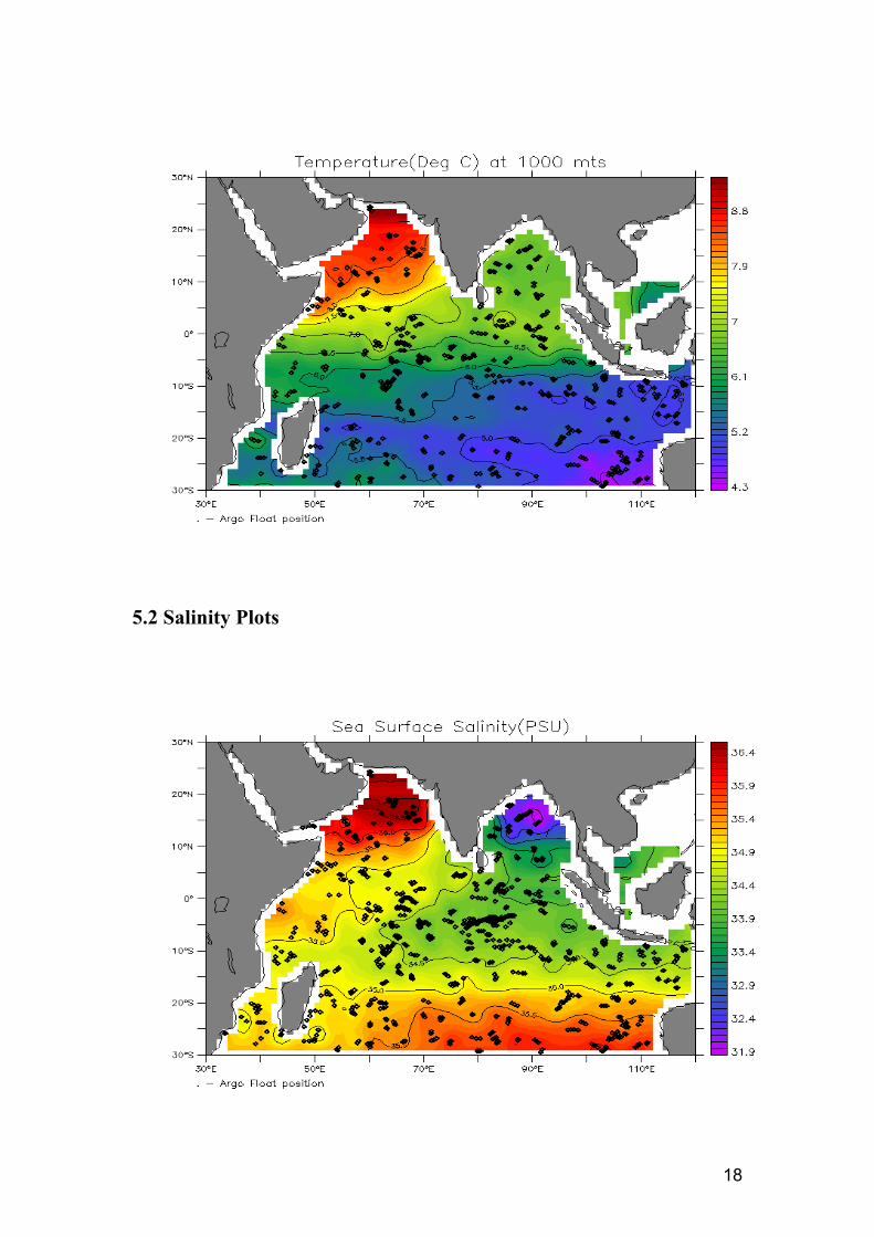
15

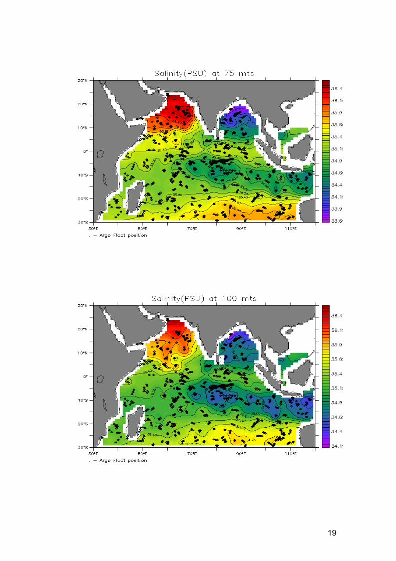
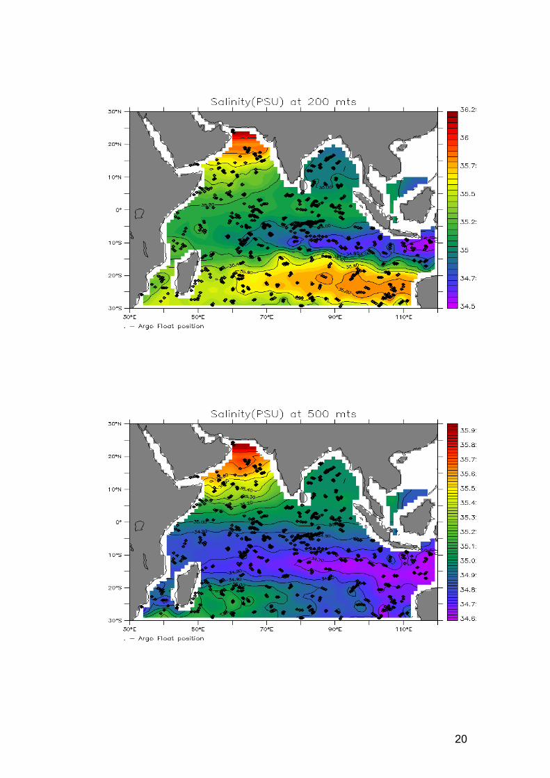
5.2

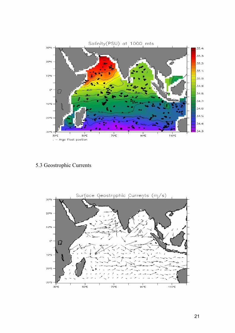
Salinity

18

5.3

Geostrophic Currents

21

3

5.4

Mixed Layer Depth, Isothermal Layer Depth

24

5.5

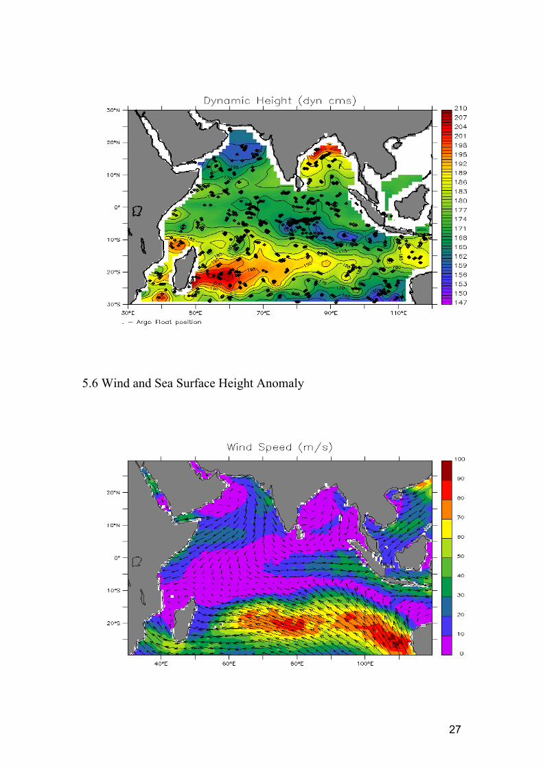
Heat Content (300 m), D20, D26, Dynamic Height

25

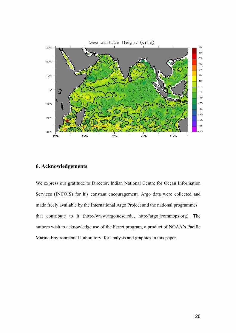
5.6

Sea Surface Height Anomaly, Wind Speed

27

6.

Acknowledgement

28

7.

References

29

8.

Appendix - 1

30

9.

Appendix - 2

31

4

1. Abstract

The system of objective analysis used at Indian National Centre for Ocean

Information Services is described. It is a integral part of the Argo data processing

system, and designed to operate with minimum of manual intervention. The analysis

method, based mainly on the method of McCreary and Kessler is a method of

estimating Gaussian weight for all the observation used for estimating the value at

grid location. The errors are determined from a comparison of the observation with

the estimated value. The analysis system is very flexible, and has been used to analyse

many different types of variables.

5

2. Introduction

A fundamental problem in the geophysical sciences is how to use data collected at

finite number of locations, and eventually at different times, to estimate value at any

point of the space or space-time continuum. The ultimate aim of such estimate can be

a simple visualization of the observed field, diagnosis of physical process of the use

of the estimated field as input for numerical models, among many other applications.

A wide set of techniques have been developed for both diagnostic and prognostic

studies/analyses. Since the development of computers in the last decades made

possible the automatic implementation of these techniques, they have been referred to

as spatial objective analysis. To put it in a nut shell Objective Analysis (OA) is the

process of transforming data from observations at irregularly spaced points into data

at points of regularly arranged grid.

2.1 Objective Analysis definition

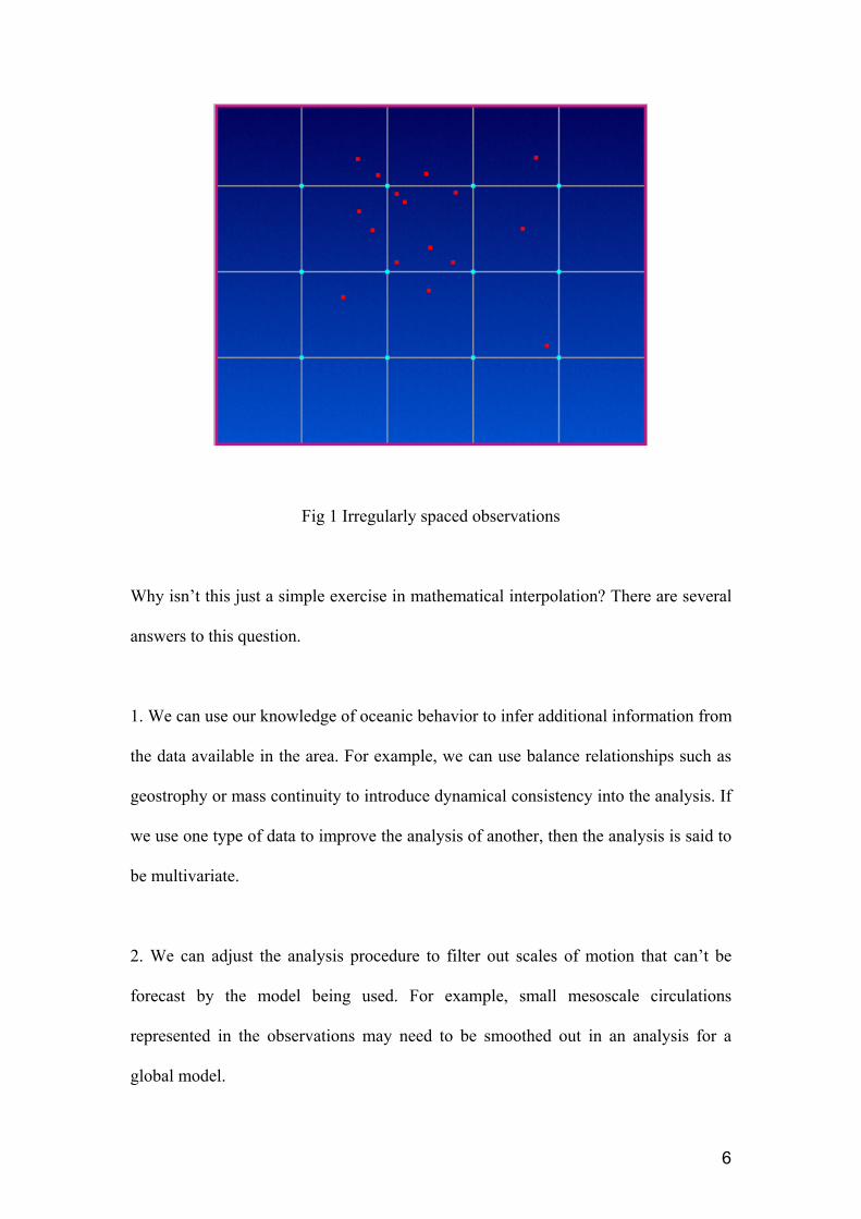
The graphic (figure 1) depicts the basic problem of OA, namely that we have

irregularly spaced observations that must provide values for points on a regularly

spaced grid. (Red dots represent observations and blue dots are grid points.) OA in

general is the process of interpolating observed values onto the grid points used by the

model/analysis in order to define the initial conditions of the atmosphere/ocean.

6

Fig 1 Irregularly spaced observations

Why isn’t this just a simple exercise in mathematical interpolation? There are several

answers to this question.

1. We can use our knowledge of oceanic behavior to infer additional information from

the data available in the area. For example, we can use balance relationships such as

geostrophy or mass continuity to introduce dynamical consistency into the analysis. If

we use one type of data to improve the analysis of another, then the analysis is said to

be multivariate.

2. We can adjust the analysis procedure to filter out scales of motion that can’t be

forecast by the model being used. For example, small mesoscale circulations

represented in the observations may need to be smoothed out in an analysis for a

global model.

7

3. We can make use of a first guess field or background field provided by an earlier

forecast from the same model. The blending of the background fields and the

observations in the objective analysis process is especially important in data sparse

areas. It allows us to avoid extrapolation of observation values into regions distant

from the observation sites. The background field can also provide detail (such as

frontal locations that exist between observations).

Using a background field also helps to introduce dynamical consistency between the

analysis and the model. In other words, that part of the analysis that comes from the

background field is already consistent with the physical (dynamic) relationships

implied by the equations used in the model.

4. We can also make use of our knowledge of the probable errors associated with each

observation. We can weight the reliability of each type of observation based on past

records of accuracy.

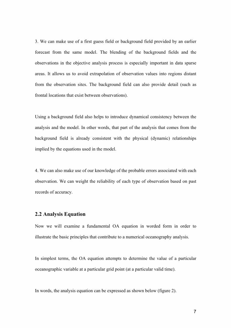
2.2 Analysis Equation

Now we will examine a fundamental OA equation in worded form in order to

illustrate the basic principles that contribute to a numerical oceanography analysis.

In simplest terms, the OA equation attempts to determine the value of a particular

oceanographic variable at a particular grid point (at a particular valid time).

In words, the analysis equation can be expressed as shown below (figure 2).

8

Fig 2 Objective Analysis equation

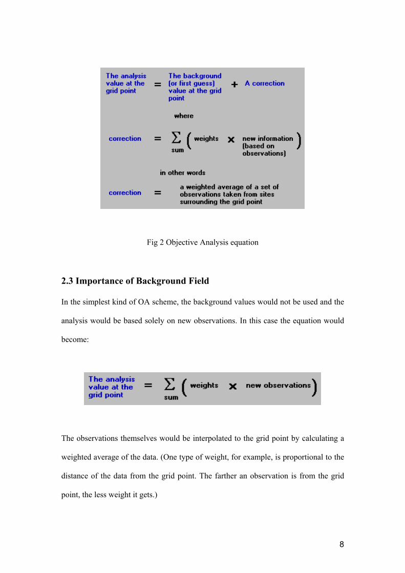
2.3 Importance of Background Field

In the simplest kind of OA scheme, the background values would not be used and the

analysis would be based solely on new observations. In this case the equation would

become:

The observations themselves would be interpolated to the grid point by calculating a

weighted average of the data. (One type of weight, for example, is proportional to the

distance of the data from the grid point. The farther an observation is from the grid

point, the less weight it gets.)

9

If a grid point has no nearby observations, the simple scheme described here is in

trouble!

3. Kessler and McCreary Methodology

3.1 Data

The data used in this analysis consisted of all the CTD data measured by Argo floats

in the Indian Ocean region (30º E – 120º E and 30º S – 30º N). The profiles’ data were

obtained from the INCOIS web site

(http://www.incois.gov.in/Incois/argo/argo_webGIS_intro.jsp#) which are made

available by USGODAE and IFREMER. Argo floats measure T/S from surface to

2000 m depth every 5/10 days. All profiles were subjected to real time quality control

checks like density inversion test, spike test and gradient test (see Wong et al., 2004).

3.2 Methodology

The gridding was carried out in two steps. First the temperature data Tn (xn, yn, zn, tn)

from each profile n were linearly interpolated to standard depths (1 m from surface to

2000 m) there by creating a modified data set T’n (xn, yn, zn, tn). This interpolation was

done only when two sample in a profile are with in a selected vertical distances which

increased from 5 m in the surface to 100 between 500 – 2000 m. Second, in a separate

computation at each Levitus standard depth Z0 (0, 10, 20, 30, 50, 75, 100, 125, 150,

200, 250, 300, 400, 500, 600, 700, 800, 900, 1000, 1200, 1400, 1600, 1800, 2000 m)

the temperature T’n were mapped from irregular grid locations (xn, yn, zn) to regular

grid (x0, y0, z0) locations with a grid spacing of 1º X 1º . Specifically the value of the

gridded temperature T’’ at each grid point (x0, y0, t0) was estimated by the operation

∑

∑

=

==p

n

p

nn

N

n

N

n

W

WTtyxT

1

1'

),,('' 000 (1)

10

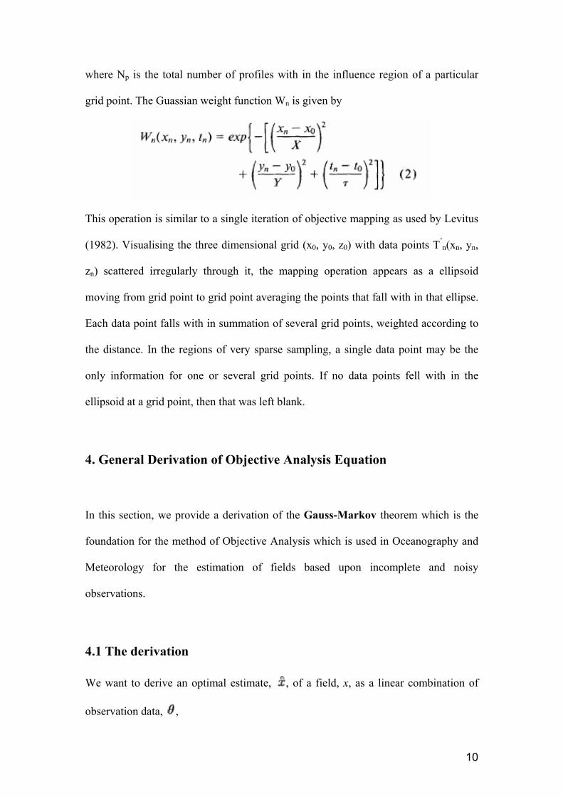
where Np is the total number of profiles with in the influence region of a particular

grid point. The Guassian weight function Wn is given by

This operation is similar to a single iteration of objective mapping as used by Levitus

(1982). Visualising the three dimensional grid (x0, y0, z0) with data points T’n(xn, yn,

zn) scattered irregularly through it, the mapping operation appears as a ellipsoid

moving from grid point to grid point averaging the points that fall with in that ellipse.

Each data point falls with in summation of several grid points, weighted according to

the distance. In the regions of very sparse sampling, a single data point may be the

only information for one or several grid points. If no data points fell with in the

ellipsoid at a grid point, then that was left blank.

4. General Derivation of Objective Analysis Equation

In this section, we provide a derivation of the Gauss-Markov theorem which is the

foundation for the method of Objective Analysis which is used in Oceanography and

Meteorology for the estimation of fields based upon incomplete and noisy

observations.

4.1 The derivation

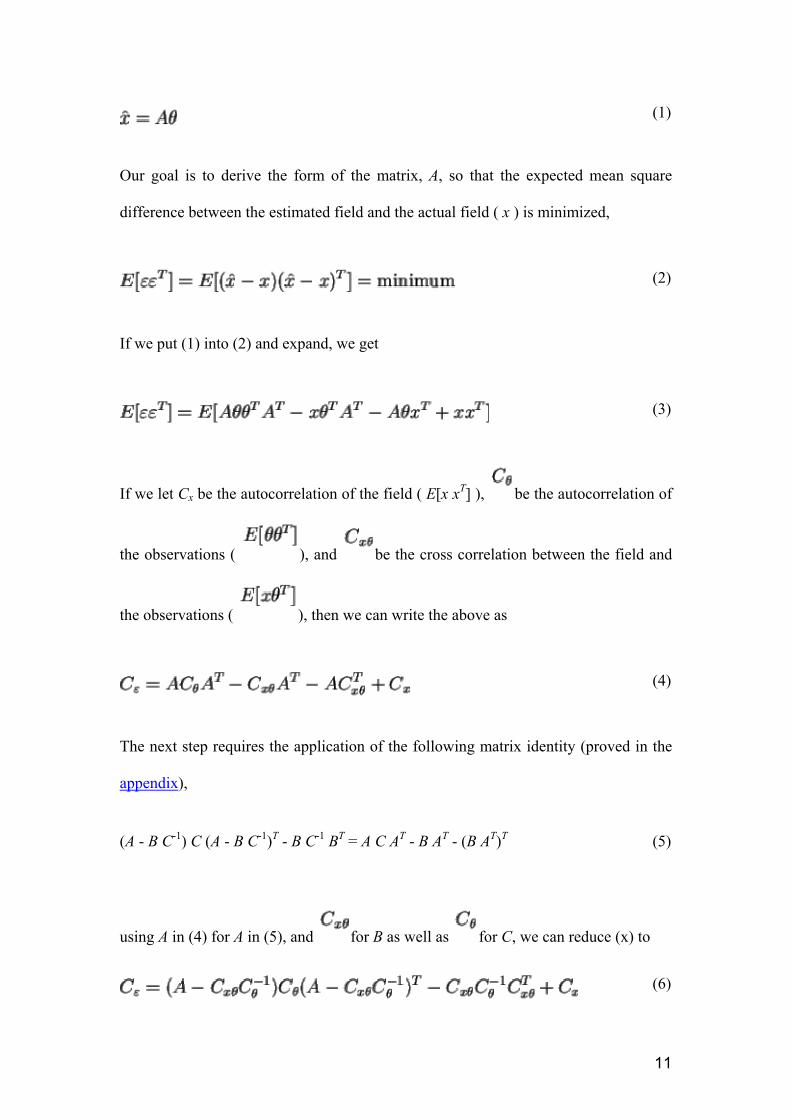
We want to derive an optimal estimate, , of a field, x, as a linear combination of

observation data, ,

11

(1)

Our goal is to derive the form of the matrix, A, so that the expected mean square

difference between the estimated field and the actual field ( x ) is minimized,

(2)

If we put (1) into (2) and expand, we get

(3)

If we let Cx be the autocorrelation of the field ( E[x xT] ), be the autocorrelation of

the observations ( ), and be the cross correlation between the field and

the observations ( ), then we can write the above as

(4)

The next step requires the application of the following matrix identity (proved in the

appendix),

(A - B C-1) C (A - B C-1)T - B C-1 BT = A C AT - B AT - (B AT)T (5)

using A in (4) for A in (5), and for B as well as for C, we can reduce (x) to

(6)

12

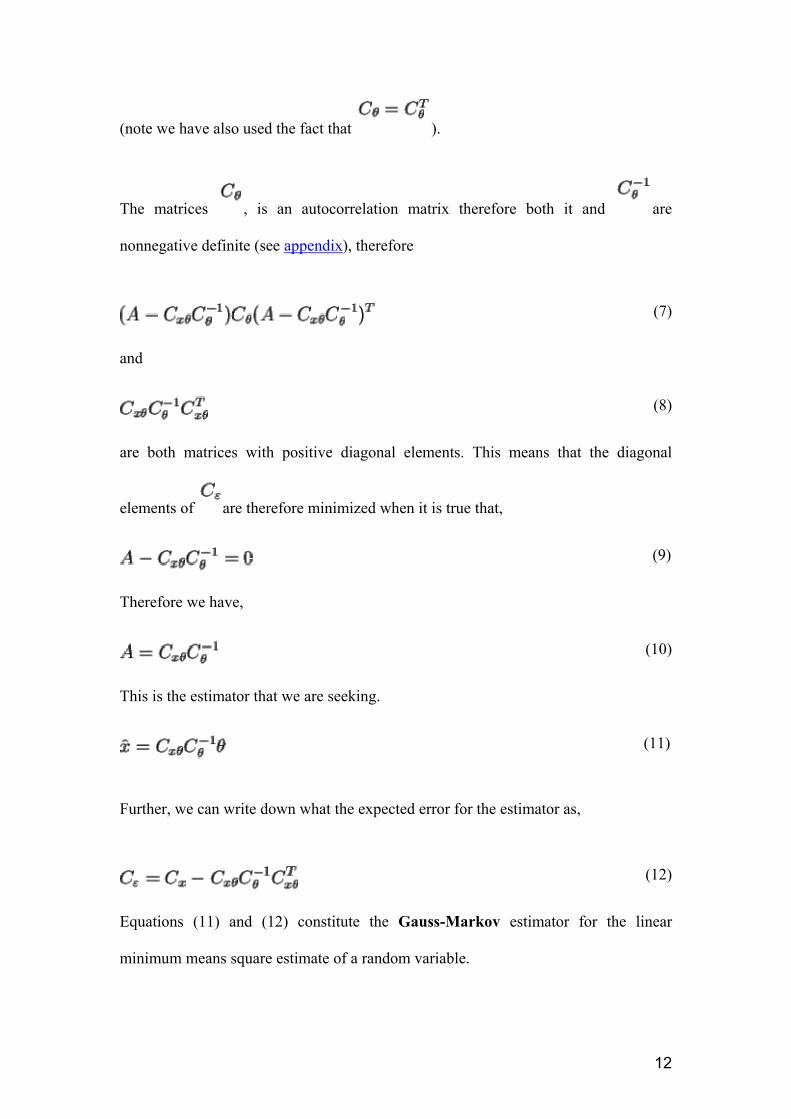
(note we have also used the fact that ).

The matrices , is an autocorrelation matrix therefore both it and are

nonnegative definite (see appendix), therefore

(7)

and

(8)

are both matrices with positive diagonal elements. This means that the diagonal

elements of are therefore minimized when it is true that,

(9)

Therefore we have,

(10)

This is the estimator that we are seeking.

(11)

Further, we can write down what the expected error for the estimator as,

(12)

Equations (11) and (12) constitute the Gauss-Markov estimator for the linear

minimum means square estimate of a random variable.

13

4.2 Linear Observations

Upon reflection of equations (11) and (12) a problem arises: the determination of

and require having the true field values, x, but all one can actually observe are

the measurement data .

In order to account for this important distinction we need to make some assumptions

about how the measurements are related to the actual state of the system. We will

assume that the observations are a linear function of the actual state plus random

noise,

(13)

where H is a known matrix that maps the data to the observations and v is the random

measurement error or noise. We introduce the index s here in order to be explicit that

we are indicating the values at some space-time location s, where the observations

are, which is not necessarily the location where the estimate of the field is being

made.

With this, we can write

(14)

Applying (13) to the definition of , gives

(15)

14

If we suppose that the actual state and the noise are uncorrelated, then the terms, Cxv

and Csv are each zero.

So now we have

(16)

and,

(17)

If we consider the case where the measurements are the same quantity as what we

are estimating x (i.e. we are using density data to estimate the density field, as

opposed to using salinity and temperature to estimate the density field), then H is just

the identity matrix, so our estimator is,

(18)

and,

(19)

If the noise is white noise, then Cv is a diagonal matrix and we see that the effect of

not having the true state correlations, but estimates of it based upon the observations,

is to increase the diagonal elements of the matrix to be inverted by the measurement

noise variance.

15

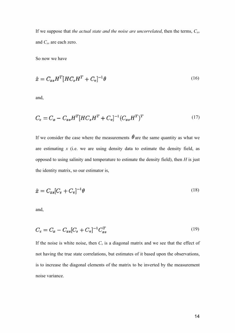
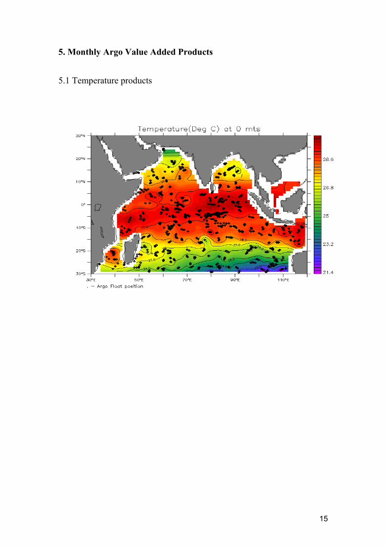
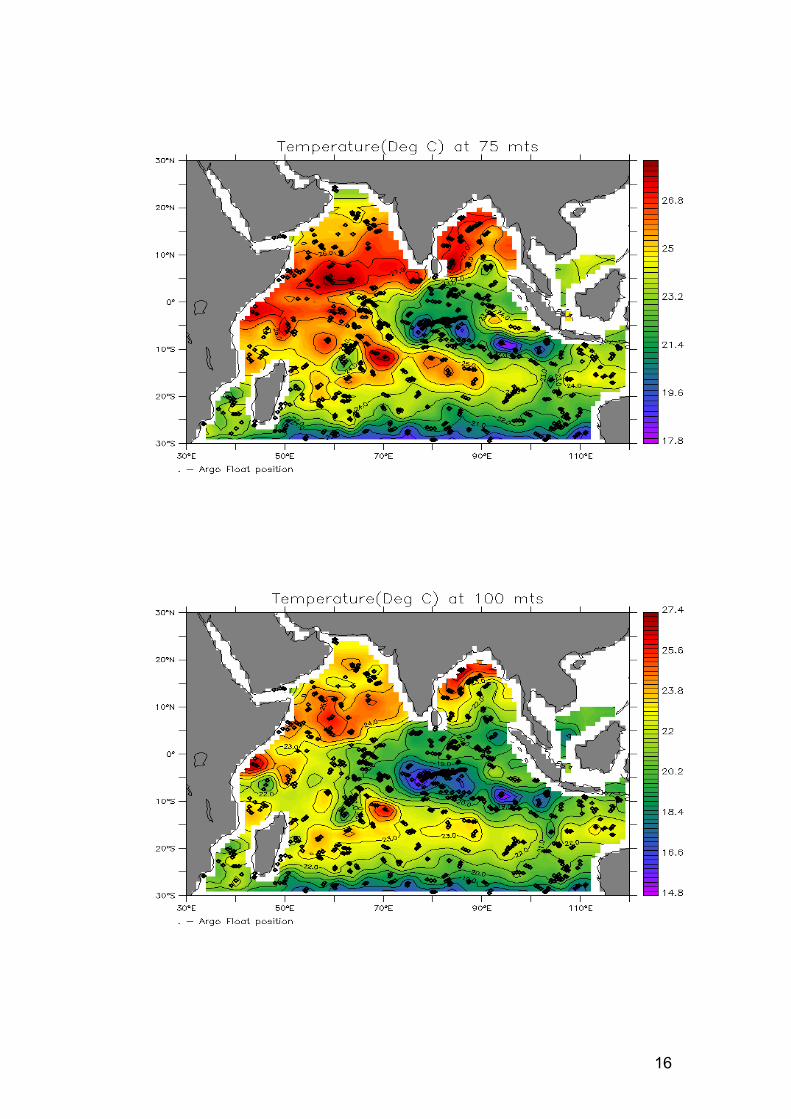
5. Monthly Argo Value Added Products

5.1 Temperature products

16

17

18

5.2 Salinity Plots

19

20

21

5.3 Geostrophic Currents

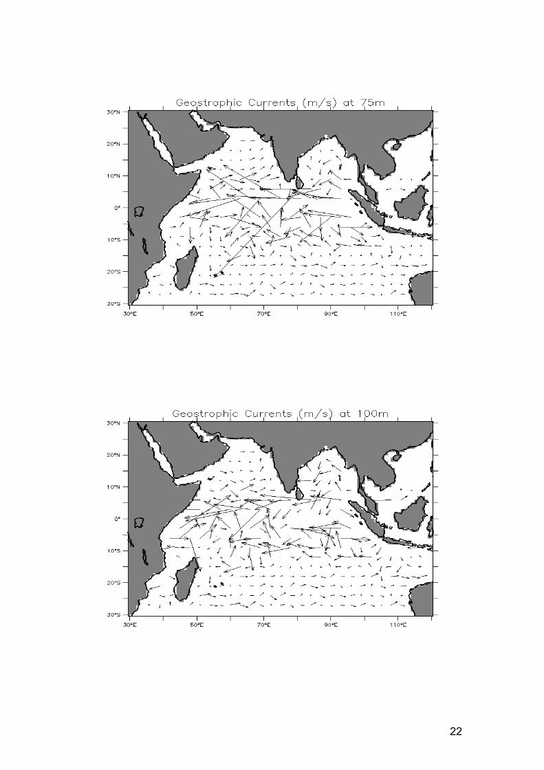
22

23

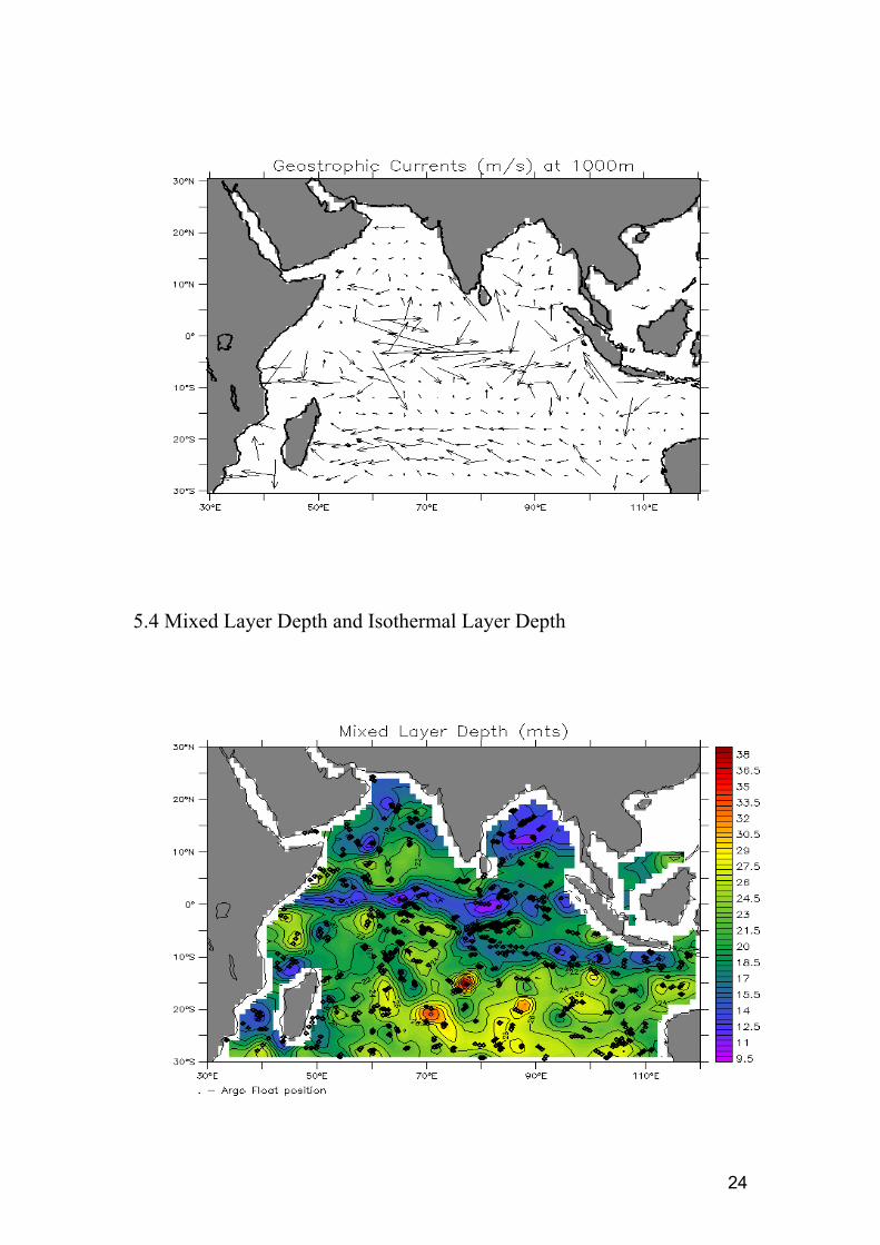
24

5.4 Mixed Layer Depth and Isothermal Layer Depth

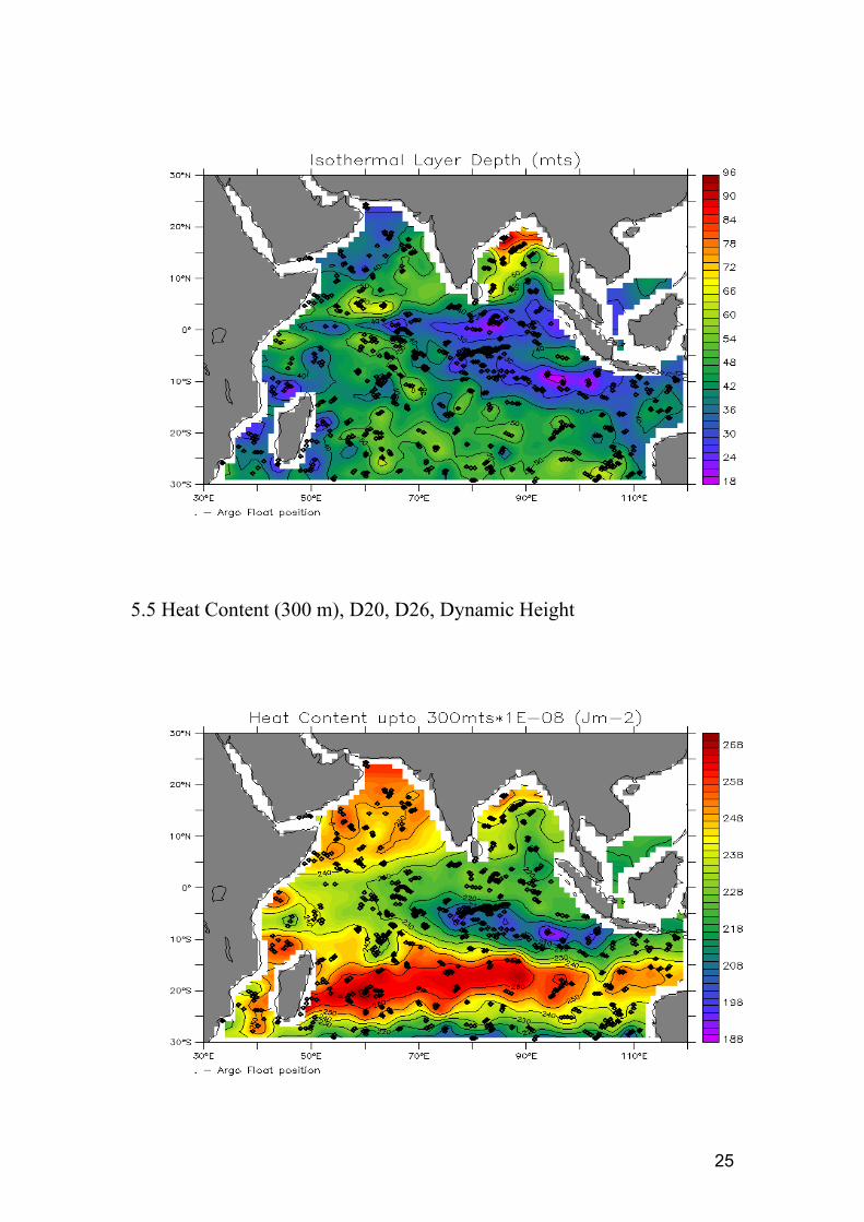
25

5.5 Heat Content (300 m), D20, D26, Dynamic Height

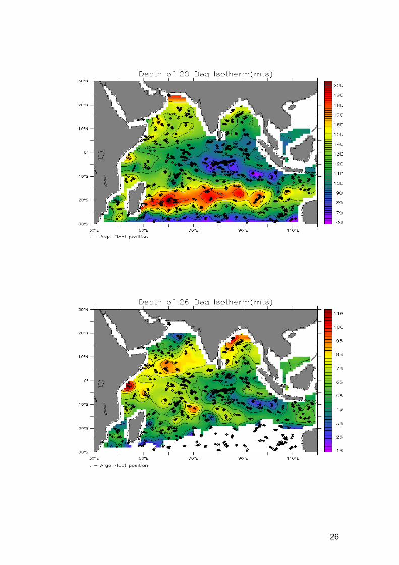
26

27

5.6 Wind and Sea Surface Height Anomaly

28

6. Acknowledgements

We express our gratitude to Director, Indian National Centre for Ocean Information

Services (INCOIS) for his constant encouragement. Argo data were collected and

made freely available by the International Argo Project and the national programmes

that contribute to it (http://www.argo.ucsd.edu, http://argo.jcommops.org). The

authors wish to acknowledge use of the Ferret program, a product of NOAA’s Pacific

Marine Environmental Laboratory, for analysis and graphics in this paper.

29

7. References

• Bretherton, F.P., R.E. Davis, and C.B. Fandry, 1976; A technique for

Objective Analysis and Design of Oceanographic Experiments applied to

MODE-73, Deep Sea Research, V 23, pp. 559-582

• Carter, E.F. and A.R. Robinson, 1987; Analysis Models for the Estimation of

Oceanic Fields, Jour. of Atmospheric and Oceanic Technology, V. 4, No. 1,

pp. 49-74

• Gandin, L.S., 1965; Objective Analysis of Meteorological Fields, Isreal

Program for Scientific Translations, Jerusaleum, 242 pages

• Liebelt, P.B., 1967; An Introduction to Optimal Estimation, Addison-Wesley,

Reading Mass., 273 pages

• Kessler and McCreary, 1993: The Annual Wind-driven Rossby Wave in the

Subthermocline Equatorial Pacific, Journal of Physical Oceanography 23,

1192 -1207.

• Wong, A., R. Keeley, T. Carval and the Argo Data Management Team. 2004.

Argo quality control manual, ver. 2.0b, Report, 23 pp.

30

8. Appendix 1

The derivation of the Gauss-Markov theorem depended upon the matrix identity,

(1)

This identity is not very intuitive and so we will provide the proof here. This proof

depends upon one assumption being true, that C = CT.

Let us define,

(2)

and,

(3)

If we can establish that , then we have our proof.

We start by expanding X,

X (A - B C-1) C (A - B C-1)T - B C-1 BT

= (A - B C-1) C (AT - C-TBT) - B C-1 BT (4)

and since we have assumed that C = CT, then C-1 = C-T, so

X = (A - B C-1) C (AT - C-1BT) - B C-1 BT

= (A C - B ) (AT - C-1BT) - B C-1 BT

= ACAT - BAT - ABT + BC-1BT - BC-1BT

=

(5)

31

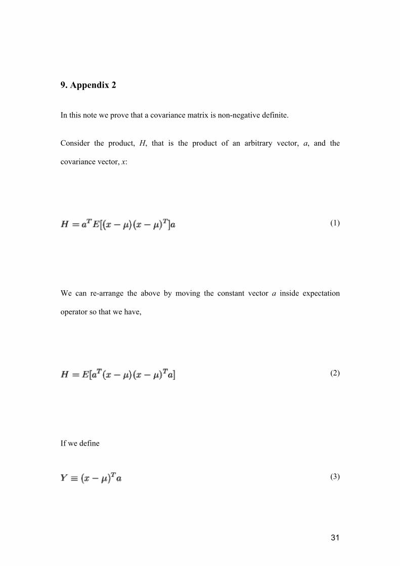
9. Appendix 2

In this note we prove that a covariance matrix is non-negative definite.

Consider the product, H, that is the product of an arbitrary vector, a, and the

covariance vector, x:

(1)

We can re-arrange the above by moving the constant vector a inside expectation

operator so that we have,

(2)

If we define

(3)

32

(which is a random variable because x is), then (2) is

H = E[ YT Y] (4)

This ``squared'' quantity is clearly never negative, so that we can conclude that the

covariance matrix is non-negative definite.