Embed Size (px)
Citation preview
AN INVESTIGATION OF REGIONAL VARIATIONS OF BARNETT SHALE
RESERVOIR PROPERTIES, AND RESULTING VARIABILITY OF
HYDROCARBON COMPOSITION AND WELL PERFORMANCE
A Thesis
by
YAO TIAN
Submitted to the Office of Graduate Studies of Texas A&M University
in partial fulfillment of the requirements for the degree of
MASTER OF SCIENCE
May 2010
Major Subject: Petroleum Engineering
AN INVESTIGATION OF REGIONAL VARIATIONS OF BARNETT SHALE
RESERVOIR PROPERTIES, AND RESULTING VARIABILITY OF
HYDROCARBON COMPOSITION AND WELL PERFORMANCE
A Thesis
by
YAO TIAN
Submitted to the Office of Graduate Studies of Texas A&M University
in partial fulfillment of the requirements for the degree of
MASTER OF SCIENCE
Approved by:
Chair of Committee, Walter B. Ayers
Committee Members, Stephen A. Holditch Yuefeng Sun Head of Department, Stephen A. Holditch
May 2010
Major Subject: Petroleum Engineering
iii
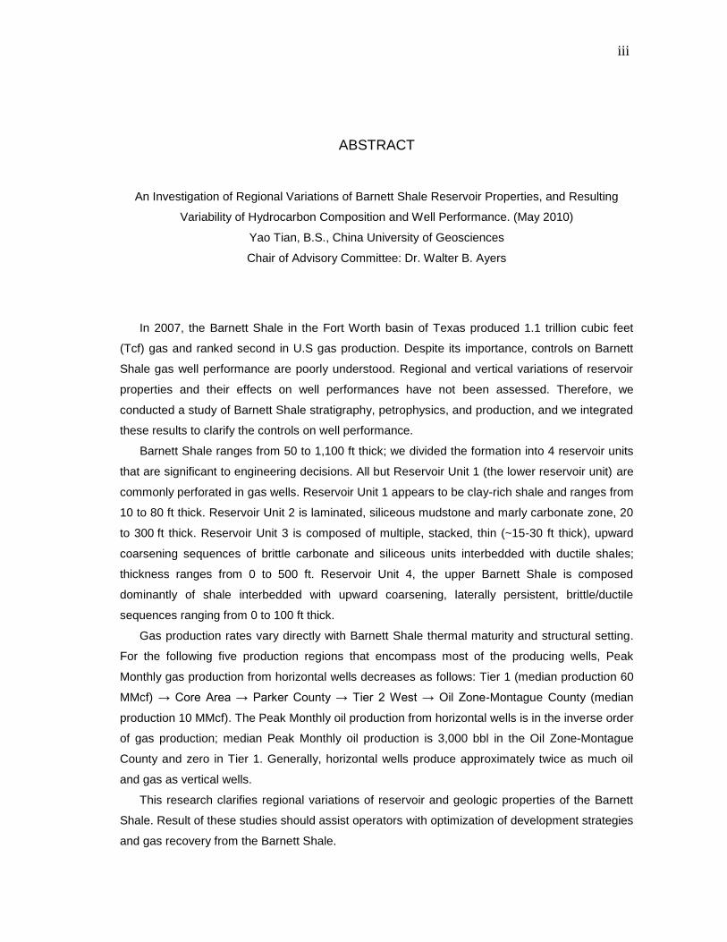
ABSTRACT
An Investigation of Regional Variations of Barnett Shale Reservoir Properties, and Resulting
Variability of Hydrocarbon Composition and Well Performance. (May 2010)
Yao Tian, B.S., China University of Geosciences
Chair of Advisory Committee: Dr. Walter B. Ayers
In 2007, the Barnett Shale in the Fort Worth basin of Texas produced 1.1 trillion cubic feet
(Tcf) gas and ranked second in U.S gas production. Despite its importance, controls on Barnett
Shale gas well performance are poorly understood. Regional and vertical variations of reservoir
properties and their effects on well performances have not been assessed. Therefore, we
conducted a study of Barnett Shale stratigraphy, petrophysics, and production, and we integrated
these results to clarify the controls on well performance.
Barnett Shale ranges from 50 to 1,100 ft thick; we divided the formation into 4 reservoir units
that are significant to engineering decisions. All but Reservoir Unit 1 (the lower reservoir unit) are
commonly perforated in gas wells. Reservoir Unit 1 appears to be clay-rich shale and ranges from
10 to 80 ft thick. Reservoir Unit 2 is laminated, siliceous mudstone and marly carbonate zone, 20
to 300 ft thick. Reservoir Unit 3 is composed of multiple, stacked, thin (~15-30 ft thick), upward
coarsening sequences of brittle carbonate and siliceous units interbedded with ductile shales;
thickness ranges from 0 to 500 ft. Reservoir Unit 4, the upper Barnett Shale is composed
dominantly of shale interbedded with upward coarsening, laterally persistent, brittle/ductile
sequences ranging from 0 to 100 ft thick.
Gas production rates vary directly with Barnett Shale thermal maturity and structural setting.
For the following five production regions that encompass most of the producing wells, Peak
Monthly gas production from horizontal wells decreases as follows: Tier 1 (median production 60
MMcf) → Core Area → Parker County → Tier 2 West → Oil Zone-Montague County (median
production 10 MMcf). The Peak Monthly oil production from horizontal wells is in the inverse order
of gas production; median Peak Monthly oil production is 3,000 bbl in the Oil Zone-Montague
County and zero in Tier 1. Generally, horizontal wells produce approximately twice as much oil
and gas as vertical wells.
This research clarifies regional variations of reservoir and geologic properties of the Barnett
Shale. Result of these studies should assist operators with optimization of development strategies
and gas recovery from the Barnett Shale.

iv
DEDICATION
To my dear advisor Dr. Walter B. Ayers
v
ACKNOWLEDGEMENTS
This research was conducted with funding from the Chrisman Institute, Halliburton Center
for Unconventional Reservoirs at Texas A&M University. I thank MJ Systems for supplying the
depth-registered image well logs used for stratigraphic analysis and appreciate IHS for providing
the digital logs. Barnett Shale gas production data were provided by HPDI.
I would like to thank my committee chair, Dr. Walter B. Ayers, and my committee
members, Dr. Stephen A. Holditch and Dr. Yuefeng Sun for their guidance and support
throughout the course of this research.
Thanks also go to my boyfriend Linfeng Bi.
vi
TABLE OF CONTENTS
Page
ABSTRACT………………………………………………………………………………………………..iii
DEDICATION……………………………………………………………………………………………...iv
ACKNOWLEDGEMENTS………………………………………………………………………………...v
TABLE OF CONTENTS ………………………………………………………………………………….vi
LIST OF FIGURES………………………………………………………………………………………viii
LIST OF TABLES…………………………………………………………………………………………xii
1. INTRODUCTION ....................................................................................................................... 1
Objectives and Methodology ............................................................................................. 3
2. REGIONAL GEOLOGY ............................................................................................................. 4
Structural Setting ............................................................................................................... 4 Stratigraphy ....................................................................................................................... 4 Barnett Shale Lithology and Reservoir Properties .......................................................... 10 Gas Resources and Reserves ......................................................................................... 14 Drilling Engineering.......................................................................................................... 15 Stimulation ....................................................................................................................... 16 Barnett Shale Regional Production Trends ..................................................................... 17
3. STRATIGRAPHIC ANALYSIS ................................................................................................. 19
Methodology .................................................................................................................... 19 Analysis of Barnett Shale Structure and Stratigraphy ..................................................... 23
4. PRODUCTION ANALYSIS ...................................................................................................... 35
Methodology .................................................................................................................... 35 Structural Setting and Thermal Maturity Controls on Regional Production Variations .... 35 Production Comparison for the Five Production Regions ............................................... 43 Perforation Interval Thickness ......................................................................................... 50 Stimulation Treatment...................................................................................................... 52 Reservoir Unit Perforated ................................................................................................ 58
5. PETROPHYSICAL ANALYSIS ................................................................................................ 61
Overview and Methodology ............................................................................................. 61 Data Preparation .............................................................................................................. 64 Single Well Petrophysical Analysis of the Barnett Shale................................................. 65 Thermal Maturity Approaches Comparison ..................................................................... 77
vii
Page
6. DISCUSSION .......................................................................................................................... 80
7. CONCLUSIONS AND RECOMMENDATIONS ....................................................................... 81
REFERENCES ............................................................................................................................. 83
APPENDIX A ................................................................................................................................ 87
VITA ............................................................................................................................................ 102
viii
LIST OF FIGURES
Page
Figure 1 Shale Gas Plays, Lower 48 States, Updated May 28, 2009. ............................... 2
Figure 2 Regional Structure of the Fort Worth Basin on Top of the Ellenburger Group. .... 5 Figure 3 Stratigraphic Column, Fort Worth Basin (Montgomery et al. 2005). .................... 6
Figure 4 Structure of the Base of the Barnett Shale Showing Exent of the Viola Limestone and Marble Falls Limestone in the Fort Worth Basin .......................... 7
Figure 5 Generalized Isopach Map of the Barnett Shale Modified from Montgomery et al. 2005.. ............................................................................................................... 9
Figure 6 Barnett Shale Mineralogy Data for Well MEC W. C. Young #2, Wise County .. 11 Figure 7 Vitrinite Reflectance of the Barnett Shale .......................................................... 13
Figure 8 Adsorption Isotherms for Barnett Shale Core Samples Recovered from the Mitchell Energy TP Sims #2 Well, Wise County.. ............................................... 14
Figure 9 EUR BCFE Equivalent for Barnett Shale Wells, by Area, in 2008. .................... 15
Figure 10 Number of Horizontal and Vertical Wells Drilled Annually in the Barnett Shale play. .................................................................................................................... 16
Figure 11 Barnett Shale Well Locations and Producing Areas. Producing Area Outlines
from (Pursell et al. 2006)... ................................................................................. 18 Figure 12 Type Well Log Showing Barnett Shale Stratigraphy and Reservoir Units
Mapped in This Study. ........................................................................................ 19 Figure 13 Locations of Wells and Cross Sections Used in This Barnett Shale Study,
Fort Worth Basin, Texas. .................................................................................... 21 Figure 14 Stratigraphic Cross Section Showing the Depositional Center of the Basin
and Identified Barnett Units 1-4. ......................................................................... 22 Figure 15 Structure, Top of the Barnett Shale. Values Are Subsea Level. ....................... 23
Figure 16 Isopach, Total Barnett Shale, Including Frostburg Ls. ....................................... 25
Figure 17 Isopach, Total Barnett Shale, Excluding Forestburg Ls. .................................... 26
Figure 18 Isopach, Forestburg Ls. The Forestburg Ls. Is Present in Only the Northeast Fort Worth Basin. ................................................................................................ 27
Figure19 Isopach, Total Lower Barnett Shale. .................................................................. 29
Figure 20 Isopach of Barnett Shale Reservoir Unit 1, Lower Hot Shale. ........................... 30
ix
Page
Figure 21 Isopach, Middle-Lower Barnett Shale RU2 Massive Carbonate Mudstone (Marl).…………...................................................................................................31
Figure 22 Isopach, Lower Barnett Shale RU3 (Upper Lower Barnett), Mainly Upward-
Coarsening Sequences. ..................................................................................... 32 Figure 23 Isopach, Upper Barnett Shale (RU4), Which Is Recognizable Where the
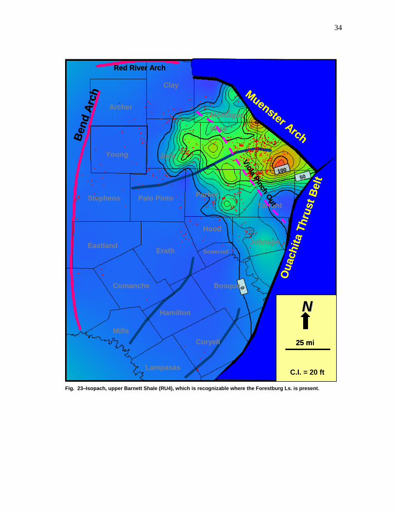
Forestburg Ls. Is Present. .................................................................................. 34 Figure 24 Structure on the Base of the Barnett Shale Showing Limits of the Viola and
Marble Falls Frac Barriers, with Overlay of Barnett Shale Gas Well Locations. 36 Figure 25 Thermal Maturity of the Barnett Shale, Showing Barnett Well Locations. from
(HPDI 2008), (modified after Montgomery et al. 2005). ..................................... 37 Figure 26 Cumulative Oil (Barrels) Produced During First Year Production Horizontal
Barnett Shale Wells. ........................................................................................... 38 Figure 27 First Year Gas Production (MMcf), Barnett Shale Horizontal Wells. .................. 39
Figure 28 Peak Monthly Gas Production (Logarithmic C.I.), Barnett Shale Horizontal Wells. .................................................................................................................. 40
Figure 29 Cumulative Gas Production, for Barnett Shale Horizontal Wells ....................... 41
Figure 30 Gas-Oil Ratio (Mcf/bbl), Barnett Shale Horizontal Wells. ................................... 42
Figure 31 Drilling Activity in Core Area.. ............................................................................. 44
Figure 32 Drilling Activity in Tier 1. ..................................................................................... 46
Figure 33 Drilling Activity in Tier 2 West. ............................................................................ 47
Figure 34 Drilling Activity in Parker County ........................................................................ 48
Figure 35 Perforation Interval Thickness and Peak Monthly Gas Production for Vertical Wells in Wise, Denton, and Tarrant County. ...................................................... 50
Figure 36 Perforation Interval Thickness and First Year Gas Production for Vertical
Wells in Wise, Denton, and Tarrant County. ...................................................... 51 Figure 37 Perforation Interval Thickness and Peak Monthly Oil Production for Vertical
Wells in Wise, Denton, and Tarrant County.. ..................................................... 51 Figure 38 Perforation Interval Thickness and First Year Oil Production for Vertical
Wells in Wise, Denton, and Tarrant County.. ..................................................... 52
Figure 39 Perforation Interval Thickness and Peak Monthly Gas Production for Vertical Wells with One Fracture Treatment and No Acid Treatment in Wise, Denton, and Tarrant County.. ........................................................................................... 53
Figure 40 Perforation Interval Thickness and Peak Monthly Gas Production for Vertical
Wells with Two Fracture Treatments and No Acid Treatment in Core Area. ..... 54
x
Page
Figure 41 Perforation Interval Thickness and First Year Gas Production for Vertical Wells with One Fracture Treatment and No Acid Treatment in Core Area.. ...... 54
Figure 42 Perforation Interval Thickness and First Year Gas Production for vertical
Wells with Two Fracture Treatments and No Acid Treatment in Wise, Denton, and Tarrant County.. ........................................................................................... 55
Figure 43 Perforation Interval Thickness and Peak Monthly Gas Production for Vertical
Wells with One Fracture Treatment and One Acid Treatment in Wise,Denton, and Tarrant County. . .......................................................................................... 56
Figure 44 Perforation Interval Thickness Peak Monthly Gas Production for Vertical
Wells with Two Fracture Treatments in Wise, Denton, and Tarrant County.. .... 56 Figure 45 Perforation Interval Thickness and First Year Gas Production for Vertical
Wells with One Fracture Treatment and One Acid Treatment in Wise, Denton, and Tarrant County.. ........................................................................................... 57
Figure 46 Perforation Interval Thickness and First Year Gas Production for Vertical
Wells with Two Fracture Treatment and One Acid Treatment in Wise, Denton, and Tarrant County.. ........................................................................................... 57
Figure 47 Group 1 Peak Monthly Gas Production between Four Types of Perforation
Approaches.. ....................................................................................................... 59 Figure 48 Group 3 Peak Monthly Gas Production between Four Types of Perforation
Approaches.. ....................................................................................................... 59 Figure 49 Comparison of Peak Monthly Oil Production between Four Types of
Perforation Approaches.. .................................................................................... 60 Figure 50 Thorium vs. Potassium Crossplot Showing the Clay Mineral Types. ................. 63
Figure 51 Locations of Wells for Which Triple Combo Logs Were Digitized.. .................... 65
Figure 52 Density vs. Neutron Porosity Crossplot for Barnett Shale Reservoir Units 1-3. 66 Figure 53 Gamma Ray vs. Neutron Porosity Crossplot for Barnett Shale Reservoir
Units 1-3.. ........................................................................................................... 67 Figure 54 Gamma Ray vs. Thorium Crossplot for Reservoir Units 1 - 3. ........................... 67
Figure 55 Gamma Ray vs. Potassium Crossplot for Barnett Reservoir Units 1 - 3. ........... 68
Figure 56 Gamma Ray vs. Uranium Crossplot for Barnett Reservoir Units 1 - 3. .............. 68
Figure 57 Thorium vs. Potassium Crossplot Showing the Clay Mineral Types for Barnett Shale Reservoir Units 1- 3. ................................................................................. 69
Figure 58 Key Petrophysical Parameters for Viola, Reservoir Unit 1 and Reservoir Unit
2. ......................................................................................................................... 70
xi
Page
Figure 59 Neutron Porosity vs. Density Cross-Plot for Reservoir Units 3 and 4 and Forestburg Limestone. ........................................................................................ 71
Figure 60 Neutron Porosity vs. Gamma Ray Crossplot for Reservoir Units 3 and 4 and
Forestburg Limestone. ................................................................................. 72
Figure 61 Thorium vs. Gamma Ray Crossplot for Reservoir Units 3 and 4 and
Forestburg Limestone. ........................................................................................ 73 Figure 62 Potassium vs. Gamma Ray Crossplot for Reservoir Units 3 and 4 and
Forestburg Limestone. ........................................................................................ 73 Figure 63 Uranium vs. Gamma Ray Crossplot for Reservoir Units 3 and 4 and
Forestburg limestone. ......................................................................................... 74 Figure 64 Thorium vs. Potassium Crossplot for Reservoir Units 3 and 4 and Forestburg
limestone. ........................................................................................................... 74 Figure 65 Fluid Analysis for Reservoir Unit 3. .................................................................... 75
Figure 66 Fluid Analysis for Reservoir Unit 4. .................................................................... 76
Figure 67 TOC Calculated from Deep Resistivity and Density Logs (TOCrd), and Density Logs (TOCd). .......................................................................................... 77
Figure 68 TOC Calculated from Density Logs vs. TOC Calculated from Deep
Resistivity and Neutron Porosity.. ...................................................................... 78 Figure 69 Uranium vs. TOC Computed from Deep Resistivity and Density Log. ............... 78
Figure 70 Uranium vs. TOC from Deep Resistivity and Neutron Porosity ......................... 79
Figure 71 Uranium vs. the Difference between Neutron and Density Porosity. ................. 79
xii
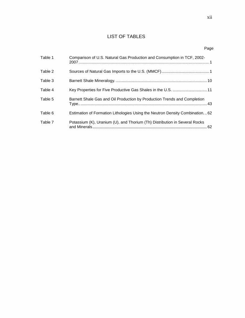
LIST OF TABLES
Page
Table 1 Comparison of U.S. Natural Gas Production and Consumption in TCF, 2002-2007 ...................................................................................................................... 1
Table 2 Sources of Natural Gas Imports to the U.S. (MMCF) ........................................... 1
Table 3 Barnett Shale Mineralogy. .................................................................................. 10
Table 4 Key Properties for Five Productive Gas Shales in the U.S. ............................... 11
Table 5 Barnett Shale Gas and Oil Production by Production Trends and Completion Type.. .................................................................................................................. 43
Table 6 Estimation of Formation Lithologies Using the Neutron Density Combination. .. 62 Table 7 Potassium (K), Uranium (U), and Thorium (Th) Distribution in Several Rocks
and Minerals ............................................................................................... 62
1
1. INTRODUCTION
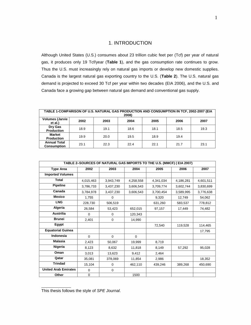
Although United States (U.S.) consumes about 23 trillion cubic feet per (Tcf) per year of natural
gas, it produces only 19 Tcf/year (Table 1), and the gas consumption rate continues to grow.
Thus the U.S. must increasingly rely on natural gas imports or develop new domestic supplies.
Canada is the largest natural gas exporting country to the U.S. (Table 2). The U.S. natural gas
demand is projected to exceed 30 Tcf per year within two decades (EIA 2006), and the U.S. and
Canada face a growing gap between natural gas demand and conventional gas supply.
TABLE 1-COMPARISON OF U.S. NATURAL GAS PRODUCTION AND CONSUMPTION IN TCF, 2002-2007 (EIA 2008)
Volumes (Jarvie et al.)
2002 2003 2004 2005 2006 2007
Dry Gas Production
18.9 19.1 18.6 18.1 18.5 19.3
Market Production
19.9 20.0 19.5 18.9 19.4
Annual Total Consumption
23.1 22.3 22.4 22.1 21.7 23.1
TABLE 2–SOURCES OF NATURAL GAS IMPORTS TO THE U.S. (MMCF) ( EIA 2007)
Type Area 2002 2003 2004 2005 2006 2007
Imported Volumes
Total 4,015,463 3,943,749 4,258,558 4,341,034 4,186,281 4,601,511
Pipeline 3,786,733 3,437,230 3,606,543 3,709,774 3,602,744 3,830,699
Canada 3,784,978 3,437,230 3,606,543 3,700,454 3,589,995 3,776,638
Mexico 1,755 0 9,320 12,749 54,062
LNG 228,730 506,519 631,260 583,537 778,812
Algeria 26,584 53,423 652,015 97,157 17,449 74,482
Austrilia 0 0 120,343
Brunei 2,401 0 14,990
Egypt 72,540 119,528 114,465
Equatorial Guinea 17,795
Indonesia 0 0 0
Malasia 2,423 50,067 19,999 8,719
Nigeria 8,123 8,632 11,818 8,149 57,292 95,028
Oman 3,013 13,623 9,412 2,464
Qatar 35,081 378,069 11,854 2,986 18,352
Trindad 15,104 0 462,110 439,246 389,268 450,690
United Arab Emirates 0 0
Other 0 1500
____________ This thesis follows the style of SPE Journal.
2
With the depletion of conventional gas reserves and growing gas demand, the development
of unconventional natural gas resources is increasingly important to future gas supply. Since
2004, unconventional gas reservoirs (tight sands, fractured shales, and coal beds) have
accounted for more than 40% of the U.S. domestic gas supply (EIA 2007).
Unconventional reservoirs were once given low priority by the oil and gas industry, because
their low permeability resulted in low production rates. However, owing to their large resources,
long-term potential, recent attractive gas prices and unprecedented interest by world markets,
unconventional gas exploration and development have increased markedly. This increased
activity and higher gas prices have led to development of new drilling, completion and stimulation
technologies, which have improved production rates and economics of unconventional gas wells.
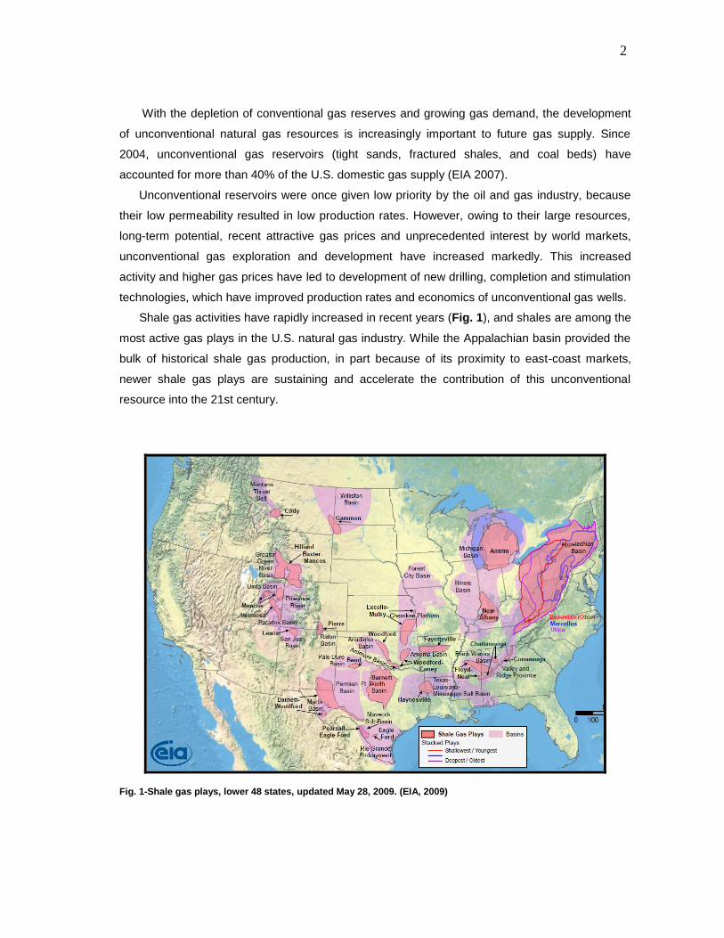
Shale gas activities have rapidly increased in recent years (Fig. 1), and shales are among the
most active gas plays in the U.S. natural gas industry. While the Appalachian basin provided the
bulk of historical shale gas production, in part because of its proximity to east-coast markets,
newer shale gas plays are sustaining and accelerate the contribution of this unconventional
resource into the 21st century.
Fig. 1-Shale gas plays, lower 48 states, updated May 28, 2009. (EIA, 2009)
3
The exploration and development of shale gas plays bring us not only new solutions to
increasing gas demand, but also the challenges of how we can economically produce gas from
low permeability reservoirs. A profitable and successful entry into a shale play requires geologists
and engineers develop an in-depth understanding of the shale reservoir.
The Barnett Shale in the Fort Worth basin of Texas is the one of the most successful shale
plays in U.S. In 2007, Newark East field produced 1.1 Tcf gas, and it ranked the second in annual
gas production in U.S. (EIA 2008). The U.S. technically recoverable shale gas resource has
increased steadily in the recent years. In 1996, the Estimated Ultimate Recovery (EUR) was
3 Tcf. With the application of horizontal drilling, in 2004, the United States Geologic Survey
estimated that the Barnett Shale in the Fort Worth basin contains 26.7 Tcf of undiscovered
natural gas, 98.5 million barrels of undiscovered oil, and 1.1 billion barrels of undiscovered
natural gas liquids (USGS 2004).
Despite its importance as the second highest producing gas field in the U.S., controls on
Barnett Shale well performance are poorly understood. The Barnett Shale is a complex, self-
sourcing reservoir, whose reservoir properties, lithology, thermal maturity, structural setting,
reservoir fluids, gas well performance, and economics vary across the Fort Worth basin. The
vertical and horizontal variations of reservoir properties and their affects on Barnett well
performances have not assessed.
Objectives and Methodology
The objectives of this study were to assess the regional and vertical variations of the Barnett
Shale reservoir properties and to evaluate the impact of these variations on reservoir production.
To accomplish these objectives, we correlated reservoir facies in a series of interlocked well logs
cross sections. Among the marker beds that were correlated are the Ellenburger top, Simpson
Group, Viola Limestone, Chappel Limestone, Barnett Shale, Forestburg Limestone, and base of
the Marble Falls Limestone. Importantly, we subdivide the Barnett Shale into 4 reservoir units
composed of 13 subdivision or sequences on the basis of gamma ray log patterns and well
perforation information. Then, we made a structure map of the top of the Barnett Shale and
isopach maps of the reservoir units.
After mapping the four Barnett Shale reservoir units, we investigated possible roles of drilling
method, structural setting, thermal maturity, perforation interval thickness, stimulation treatment
and reservoir unit perforated to assess controls on Barnett Shale fluid composition and production
rates. Also, we investigated the petrophysical characteristics of each unit and assessed the
vertical variations of these properties among the reservoir unit.
4
2. REGIONAL GEOLOGY
Structural Setting
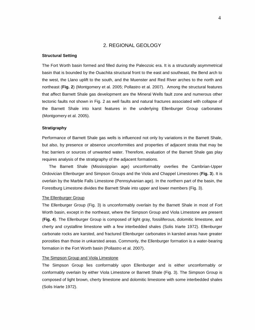
The Fort Worth basin formed and filled during the Paleozoic era. It is a structurally asymmetrical
basin that is bounded by the Ouachita structural front to the east and southeast, the Bend arch to
the west, the Llano uplift to the south, and the Muenster and Red River arches to the north and
northeast (Fig. 2) (Montgomery et al. 2005; Pollastro et al. 2007). Among the structural features
that affect Barnett Shale gas development are the Mineral Wells fault zone and numerous other
tectonic faults not shown in Fig. 2 as well faults and natural fractures associated with collapse of
the Barnett Shale into karst features in the underlying Ellenburger Group carbonates
(Montgomery et al. 2005).
Stratigraphy
Performance of Barnett Shale gas wells is influenced not only by variations in the Barnett Shale,
but also, by presence or absence unconformities and properties of adjacent strata that may be
frac barriers or sources of unwanted water. Therefore, evaluation of the Barnett Shale gas play
requires analysis of the stratigraphy of the adjacent formations.
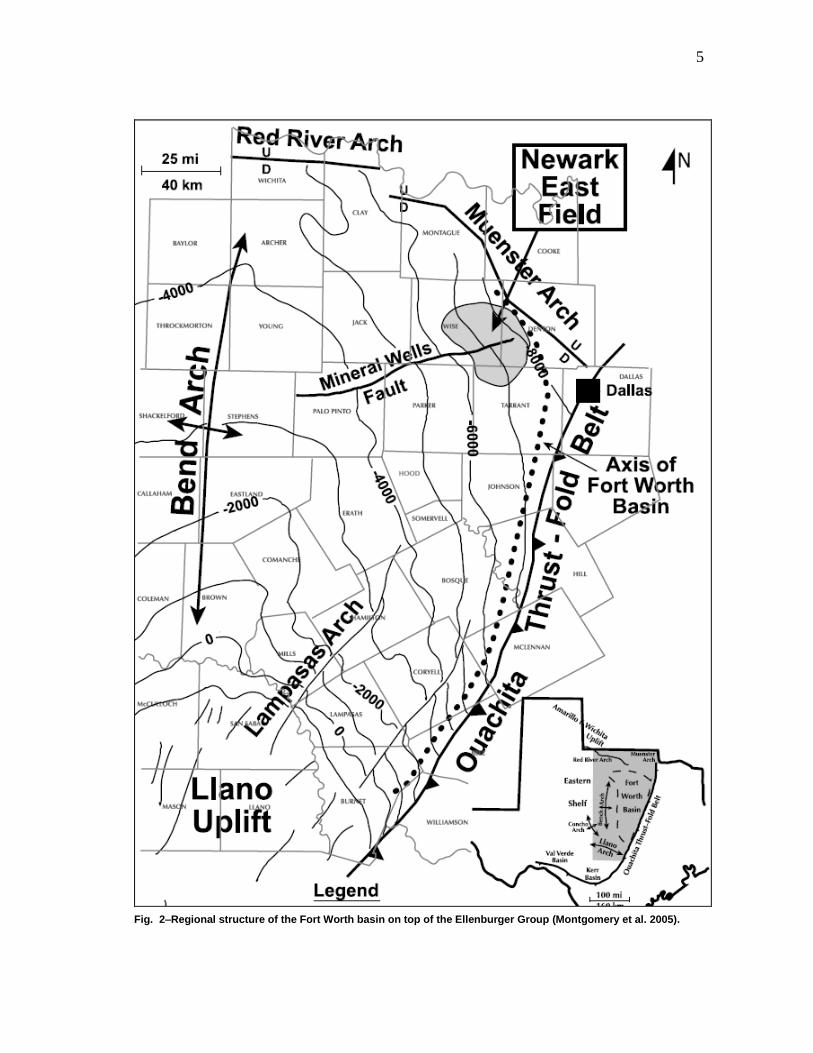
The Barnett Shale (Mississippian age) unconformably overlies the Cambrian-Upper
Ordovician Ellenburger and Simpson Groups and the Viola and Chappel Limestones (Fig. 3). It is
overlain by the Marble Falls Limestone (Pennsylvanian age). In the northern part of the basin, the
Forestburg Limestone divides the Barnett Shale into upper and lower members (Fig. 3).
The Ellenburger Group
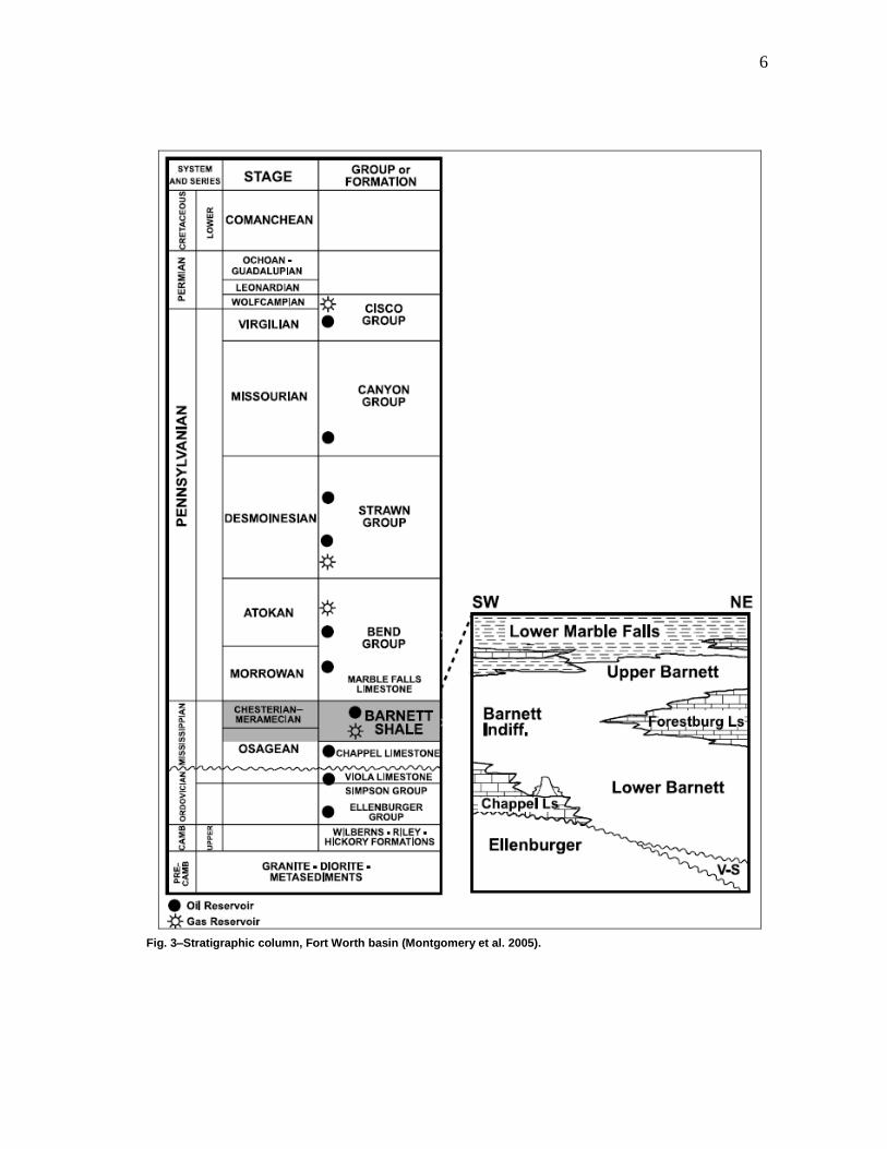
The Ellenburger Group (Fig. 3) is unconformably overlain by the Barnett Shale in most of Fort
Worth basin, except in the northeast, where the Simpson Group and Viola Limestone are present
(Fig. 4). The Ellenburger Group is composed of light gray, fossiliferous, dolomitic limestone, and
cherty and crystalline limestone with a few interbedded shales (Solis Iriarte 1972). Ellenburger
carbonate rocks are karsted, and fractured Ellenburger carbonates in karsted areas have greater
porosities than those in unkarsted areas. Commonly, the Ellenburger formation is a water-bearing
formation in the Fort Worth basin (Pollastro et al. 2007).
The Simpson Group and Viola Limestone
The Simpson Group lies conformably upon Ellenburger and is either unconformably or
conformably overlain by either Viola Limestone or Barnett Shale (Fig. 3). The Simpson Group is
composed of light brown, cherty limestone and dolomitic limestone with some interbedded shales
(Solis Iriarte 1972).
5
Fig. 2–Regional structure of the Fort Worth basin on top of the Ellenburger Group (Montgomery et al. 2005).
6
Fig. 3–Stratigraphic column, Fort Worth basin (Montgomery et al. 2005).
7
Fig. 4–Structure of the base of the Barnett Shale showing extent of the Viola Limestone and Marble Falls Limestone in the Fort Worth basin ( modified after Givens and Zhao 2004).
The Viola Limestone conformably overlies the Simpson Group and is unconformably overlain
by the Barnett Shale (Fig. 3). It is divided into a lower unit, which composed of light gray
limestone with shale intercalations, and an upper unit that is composed of coarse gray limestone.
8
The Viola Limestone is present in only the northeast part of the Fort Worth Basin (Fig. 4), where it
attains a maximum thickness of 170 feet in Tarrant County (Solis Iriarte 1972).
The Chappel Limestone
The Mississippian-age Chappel Limestone (Fig. 3) underlies or intertongues with the Barnett
Shale in the western and northern parts of the Fort Worth Basin. The Chappel Limestone is
comprised of reef core and inter-reef facies. Generally, Chappel reef deposits are thicker and
older towards the northeast, in Jack County. They are typically 100-150 ft, but four known reefs in
Montague County are as much as 350 ft thick (Henry 1982).
Barnett Shale and Forestburg Limestone
The Barnett Shale unconformably overlies the Viola Limestone or Ellenburger Group, and it is
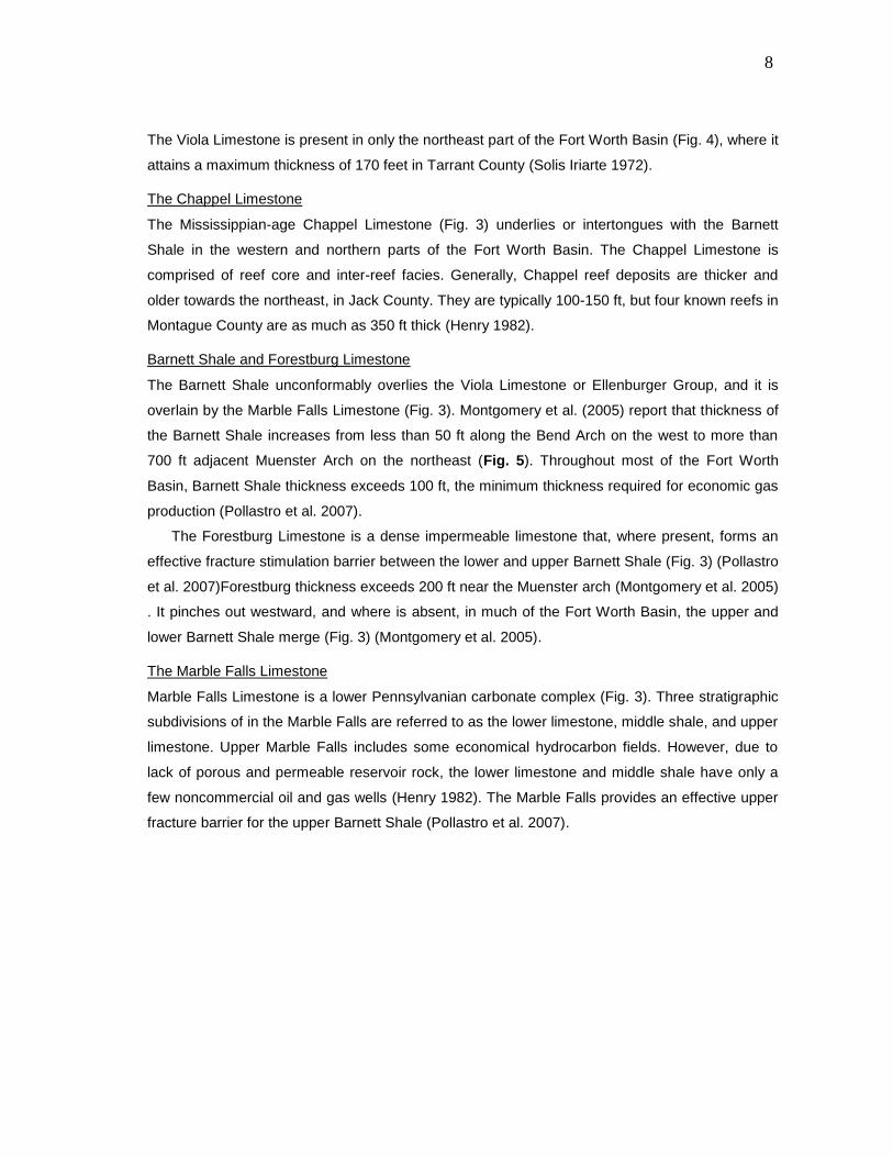
overlain by the Marble Falls Limestone (Fig. 3). Montgomery et al. (2005) report that thickness of
the Barnett Shale increases from less than 50 ft along the Bend Arch on the west to more than
700 ft adjacent Muenster Arch on the northeast (Fig. 5). Throughout most of the Fort Worth
Basin, Barnett Shale thickness exceeds 100 ft, the minimum thickness required for economic gas
production (Pollastro et al. 2007).
The Forestburg Limestone is a dense impermeable limestone that, where present, forms an
effective fracture stimulation barrier between the lower and upper Barnett Shale (Fig. 3) (Pollastro
et al. 2007)Forestburg thickness exceeds 200 ft near the Muenster arch (Montgomery et al. 2005)
. It pinches out westward, and where is absent, in much of the Fort Worth Basin, the upper and
lower Barnett Shale merge (Fig. 3) (Montgomery et al. 2005).
The Marble Falls Limestone
Marble Falls Limestone is a lower Pennsylvanian carbonate complex (Fig. 3). Three stratigraphic
subdivisions of in the Marble Falls are referred to as the lower limestone, middle shale, and upper
limestone. Upper Marble Falls includes some economical hydrocarbon fields. However, due to
lack of porous and permeable reservoir rock, the lower limestone and middle shale have only a
few noncommercial oil and gas wells (Henry 1982). The Marble Falls provides an effective upper
fracture barrier for the upper Barnett Shale (Pollastro et al. 2007).
9
Fig. 5–Generalized isopach map of the Barnett Shale Modified from Montgomery et al. 2005.
10
Barnett Shale Lithology and Reservoir Properties
Lithology
The Barnett Shale was deposited in marine shelf and deep-water settings in the remnant of a
Paleozoic aulacogen in north-central Texas (Montgomery et al. 2005). The name Barnett “Shale”
may be misleading, because the mineral composition of the formation is highly variable, and in
many cases, the formation is not a true shale. Analyses of Barnett Shale samples from Wise and
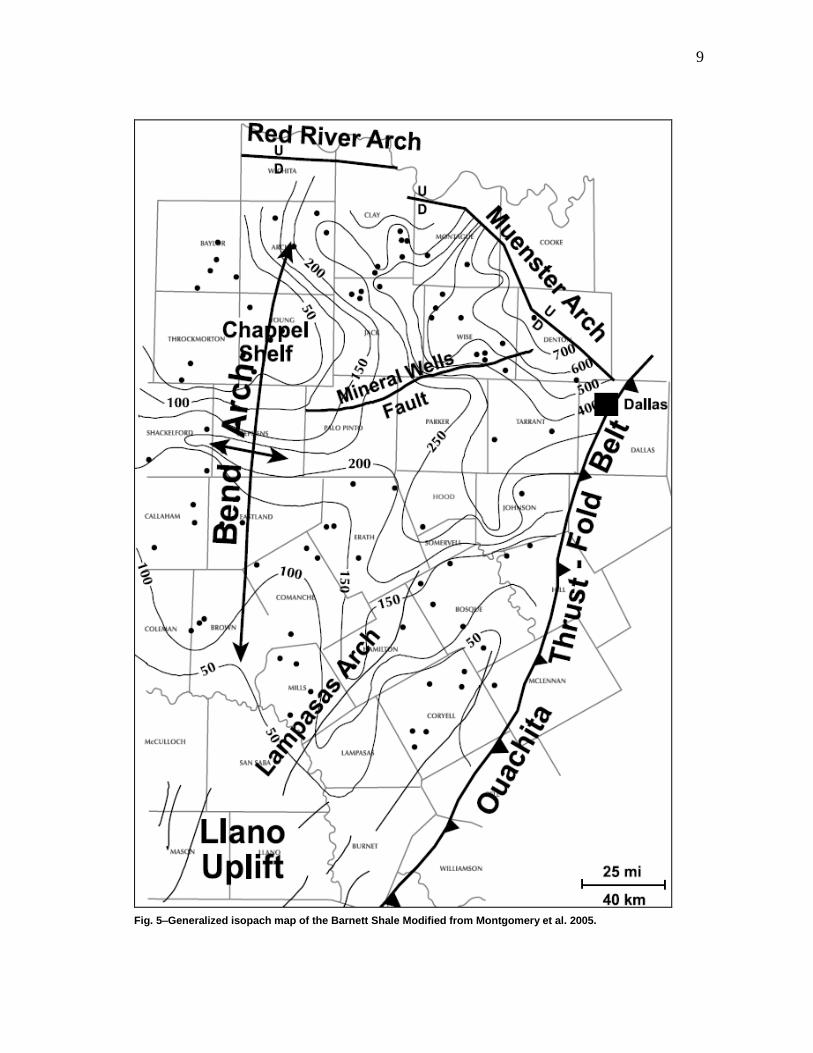
Denton Counties indicate that, in the core area, average Barnett Shale composition is 45–55% silt
(quartz and feldspar), 15–25% carbonate, 20–35% clay minerals, and 2–6% pyrite, by weight
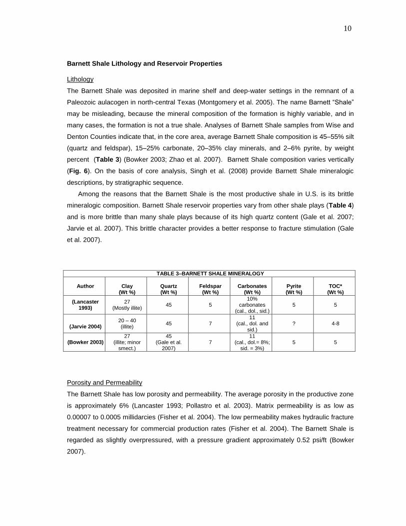
percent (Table 3) (Bowker 2003; Zhao et al. 2007). Barnett Shale composition varies vertically
(Fig. 6). On the basis of core analysis, Singh et al. (2008) provide Barnett Shale mineralogic
descriptions, by stratigraphic sequence.
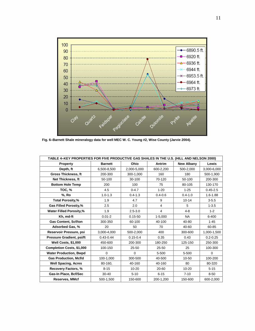
Among the reasons that the Barnett Shale is the most productive shale in U.S. is its brittle
mineralogic composition. Barnett Shale reservoir properties vary from other shale plays (Table 4)
and is more brittle than many shale plays because of its high quartz content (Gale et al. 2007;
Jarvie et al. 2007). This brittle character provides a better response to fracture stimulation (Gale
et al. 2007).
TABLE 3–BARNETT SHALE MINERALOGY
Author
Clay (Wt %)
Quartz (Wt %)
Feldspar (Wt %)
Carbonates
(Wt %)
Pyrite (Wt %)
TOC*
(Wt %)
(Lancaster 1993)
27 (Mostly illite)
45 5 10%
carbonates (cal., dol., sid.)
5 5
(Jarvie 2004)
20 – 40 (illite)
45 7 11
(cal., dol. and sid.)
? 4-8
(Bowker 2003) 27
(illite; minor smect.)
45 (Gale et al.
2007) 7
11 (cal., dol.= 8%;
sid. = 3%) 5 5
Porosity and Permeability
The Barnett Shale has low porosity and permeability. The average porosity in the productive zone
is approximately 6% (Lancaster 1993; Pollastro et al. 2003). Matrix permeability is as low as
0.00007 to 0.0005 millidarcies (Fisher et al. 2004). The low permeability makes hydraulic fracture
treatment necessary for commercial production rates (Fisher et al. 2004). The Barnett Shale is
regarded as slightly overpressured, with a pressure gradient approximately 0.52 psi/ft (Bowker
2007).
11
Fig. 6–Barnett Shale mineralogy data for well MEC W. C. Young #2, Wise County (Jarvie 2004).
TABLE 4–KEY PROPERTIES FOR FIVE PRODUCTIVE GAS SHALES IN THE U.S. (HILL AND NELSON 2000)
Property Barnett Ohio Antrim New Albany Lewis
Depth, ft 6,500-8,500 2,000-5,000 600-2,200 500-2,000 3,000-6,000
Gross Thickness, ft 200-300 300-1,000 160 180 500-1,900
Net Thickness, ft 50-100 30-100 70-120 50-100 200-300
Bottom Hole Temp 200 100 75 80-105 130-170
TOC, % 4.5 0-4.7 1-20 1-25 0.45-2.5
%, Ro 1.0-1.3 0.4-1.3 0.4-0.6 0.4-1.0 1.6-1.88
Total Porosity,% 1.9 4.7 9 10-14 3-5.5
Gas Filled Porostiy,% 2.5 2.0 4 5 1-3.5
Water Filled Porosity,% 1.9 2.5-3.0 4 4-8 1-2
Kh, md-ft 0.01-2 0.15-50 1-5,000 NA 6-400
Gas Content, Scf/ton 300-350 60-100 40-100 40-80 1-45
Adsorbed Gas, % 20 50 70 40-60 60-85
Reservoir Pressure, psi 3,000-4,000 500-2,000 400 300-600 1,000-1,500
Pressure Gradient, psi/ft 0.43-0.44 0.15-0.4 0.35 0.43 0.2-0.25
Well Costs, $1,000 450-600 200-300 180-250 125-150 250-300
Completion Costs, $1,000 100-150 25-50 25-50 25 100-300
Water Production, Bwpd 0 0 5-500 5-500 0
Gas Production, Mcf/d 100-1,000 300-500 40-500 10-50 100-200
Well Spacing, Acres 80-160, 40-160 40-160 80 80-320
Recovery Factors, % 8-15 10-20 20-60 10-20 5-15
Gas-In Place, Bcf/Sec 30-40 5-10 6-15 7-10 8-50
Reserves, MMcf 500-1,500 150-600 200-1,200 150-600 600-2,000
12
Natural Fractures
The Barnett Shale is a naturally fractured reservoir. The primary natural fracture system trends
northwestward, parallel to the faulted Muenster arch, and it dips 74º to the southwest
(Montgomery et al. 2005). A secondary fracture set is oriented north-south (Gale et al. 2007). Dip
of the natural fractures is generally steep, and fracture apertures are generally less than 0.002
inches wide (Bowker 2007). The fractures have length/width aspect ratios greater than 1000:1
(Gale et al. 2007). Core samples indicate that many of the natural fractures are cemented by
calcite (Gale et al. 2007). The role of natural fractures in Barnett well production performance is
disputed (Bowker 2003; Bowker 2007; Montgomery et al. 2005). Some authors report that natural
fractures improve production, whereas others report that they are rarely present, and if present,
they are closed due to the mineralization.
Geochemistry
Knowledge of organic richness, gas content, kerogen type, and extent of kerogen transformation
is critical for evaluating shale-gas potential (Jarvie 2004). The Barnett total organic carbon (TOC)
was reported for two types of samples. Mean TOC values from multiple well cutting samples
range between 1 and 5 wt.% and are more commonly between 2.5 and 3.5 wt.%. For core
samples, Barnett Shale TOC is commonly higher, generally 4–5 wt.% (Bowker 2003; Montgomery
et al. 2005).
Geochemical evidence indicates that oil and gas in many Fort Worth Basin reservoirs
originated from the Barnett Shale. The Barnett Shale contains primarily Type II (oil-prone)
kerogen that was deposited under normal-marine salinities and dysoxic conditions (Jarvie 2004).
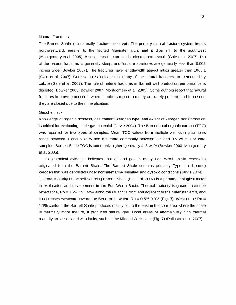
Thermal maturity of the self-sourcing Barnett Shale (Hill et al. 2007) is a primary geological factor
in exploration and development in the Fort Worth Basin. Thermal maturity is greatest (vitrinite
reflectance, Ro = 1.2% to 1.9%) along the Quachita front and adjacent to the Muenster Arch, and
it decreases westward toward the Bend Arch, where Ro = 0.5%-0.9% (Fig. 7). West of the Ro =
1.1% contour, the Barnett Shale produces mainly oil; to the east in the core area where the shale
is thermally more mature, it produces natural gas. Local areas of anomalously high thermal
maturity are associated with faults, such as the Mineral Wells fault (Fig. 7) (Pollastro et al. 2007).
13
Fig. 7–Vitrinite reflectance of the Barnett Shale (modified after Montgomery et al. 2005).
14
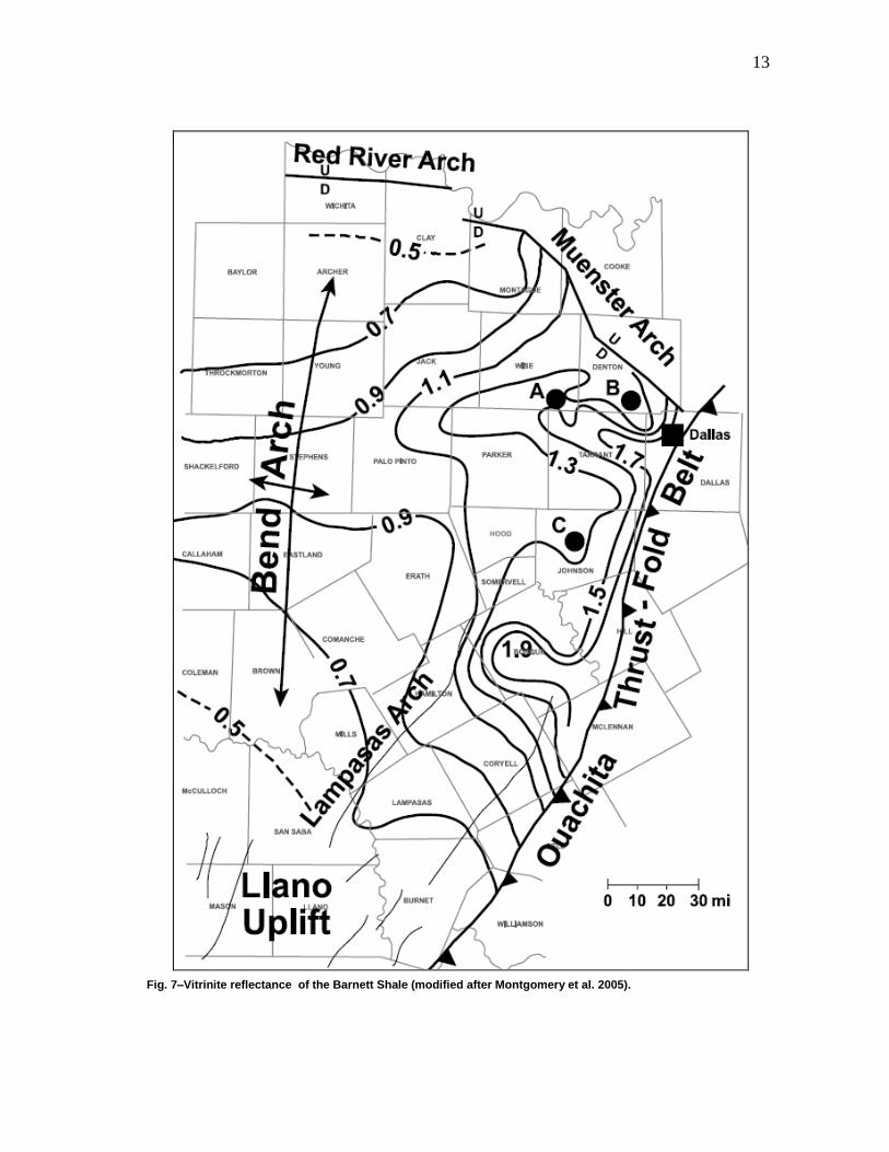
Gas Content and Occurrence
Natural gas in the Barnett Shale is stored as free gas or absorbed gas. Free gas is compressed
in the natural fractures and in macropores of fine clastic sediment, whereas absorbed gas is
bound to organic matter in the shale matrix (Fig. 8) (Montgomery et al. 2005). Mavor (2003)
reported Barnett Shale gas content in Wise County was 196.7 scf/t; more than half of the gas
(120 scf/t) was absorbed. However, research indicates that, in Wise county, average total Barnett
Shale gas is 191 scf/ton; this includes 88 scf/ton (48%) sorbed gas and 103 scf/ton (52%) free
gas (Jarvie 2004).
Fig. 8–Adsorption isotherms for Barnett Shale core samples recovered from the Mitchell Energy TP Sims #2 well, Wise County. Sorbed gas content ranges from 60-125 scf/t and total gas content ranges from 170-250 at a reservoir pressure of 3,800 psi (Montgomery et al. 2005).
Gas Resources and Reserves
Reportedly, the Barnett Shale holds 26.2 Tcf of undiscovered natural gas (USGS 2004).
Estimated Ultimate Recovery (EUR) for Barnett Shale wells has increased with time. Before
1990, EUR was 0.3-0.5 Bcf/well. Between 1990 and 1997, EUR ranged from 0.6 to 1.0 Bcf/well,
and it increased to 0.8-1.2 Bcf/well between 1998 and 2000. Beginning in 2002, with widespread
15
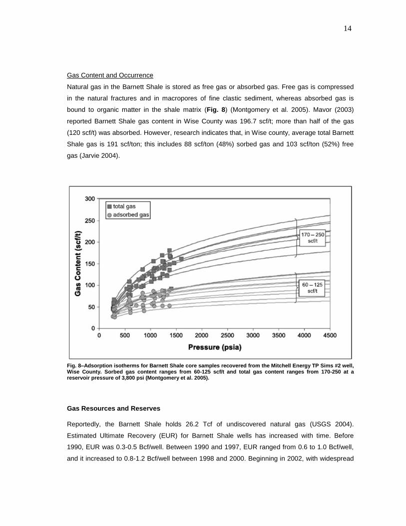
application of horizontal drilling in the Barnett Shale, the average EUR increased markedly
(Daniels et al. 2007). By 2008, the average EUR had increased to 2.2 Bcf/well in the Primary
Area (Fig. 9) (Devon Energy 2008).
Drilling Engineering
Initial development of the Barnett Shale in the 1990s was by vertical wells in the lower Barnett
Shale. However, low flow rates and EURs led the industry to use other drilling techniques.
Horizontal drilling started in earnest in 2002, after Devon Energy acquired Mitchell Energy (Devon
Energy 2008). Horizontal wells offer the benefit of increasing the EUR by three times with only a
doubling of the well cost (Waters et al. 2006). Horizontal drilling reduces the probability of vertical
fracture growth into nearby aquifers. Also, horizontal wells can access surface locations that
present challenges to vertical drilling, such as areas beneath houses and airports, and they
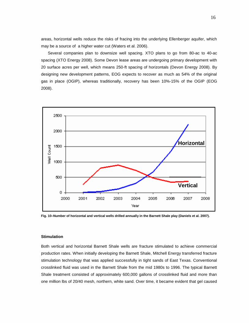
minimize the surface footprint of development (Fisher et al. 2004). Since late 2004, there have
been more horizontal wells than vertical Barnett wells drilled annually (Fig. 10).
Fig. 9–EUR BCFE (billion cubic feet) equivalent for Barnett Shale wells, by area, in 2008 (Devon Energy 2008).
Among the greatest impacts of horizontal drilling is the advantage that it offers relative to
vertical drilling in areas where the Viola Limestone frac barrier is absent (Figs. 3 and 4). In those
16
areas, horizontal wells reduce the risks of fracing into the underlying Ellenberger aquifer, which
may be a source of a higher water cut (Waters et al. 2006).
Several companies plan to downsize well spacing. XTO plans to go from 80-ac to 40-ac
spacing (XTO Energy 2008). Some Devon lease areas are undergoing primary development with
20 surface acres per well, which means 250-ft spacing of horizontals (Devon Energy 2008). By
designing new development patterns, EOG expects to recover as much as 54% of the original
gas in place (OGIP), whereas traditionally, recovery has been 10%-15% of the OGIP (EOG
2008).
Horizontal
Vertical
Horizontal
Vertical
Fig. 10–Number of horizontal and vertical wells drilled annually in the Barnett Shale play (Daniels et al. 2007).
Stimulation
Both vertical and horizontal Barnett Shale wells are fracture stimulated to achieve commercial
production rates. When initially developing the Barnett Shale, Mitchell Energy transferred fracture
stimulation technology that was applied successfully in tight sands of East Texas. Conventional
crosslinked fluid was used in the Barnett Shale from the mid 1980s to 1996. The typical Barnett
Shale treatment consisted of approximately 600,000 gallons of crosslinked fluid and more than
one million lbs of 20/40 mesh, northern, white sand. Over time, it became evident that gel caused
17
reservoir damage (Waters et al. 2006). As a result, the preferred stimulation method evolved to a
more effective and less damaging water frac technique (Fisher et al. 2004).
The success of slick water fracturing in Cotton Valley sand in East Texas in 1997 led Mitchell
Energy to experiment with this stimulation method in the Barnett Shale in 1998 (Fisher et al.
2004; Matthews et al. 2007). This treatment consists of twice the fluid volume that was used for
the crosslinked treatment, but less than 10% of that proppant volume. While there is no drastic
production increasing as a result of this stimulation method, costs were reduced by approximately
65%. This cost reduction allowed the economic addition of completions in the Upper Barnett
Shale in Denton and Wise counties, which increased the EUR by 20 to 25 % (Matthews et al.
2007; Waters et al. 2006).
Three advantages of the high-rate, large-volume, and low-sand-concentration water frac
treatments in the Barnett Shale are greater lateral extent, higher conductivity, and reduced
damage from gel(East et al. 2004). The Barnett Shale is suitable for water frac because of its
mineralogy and presence of natural fractures. The mineralogy causes certain zones of the
Barnett Shale to be brittle, and thus, easier to be fracture stimulated (Montgomery et al. 2005).
The interaction of induced fractures with natural fractures systems results in complex networks of
induced and natural fracture that connect large matrix volumes to the wellbore.
Horizontal Barnett wells are usually drilled to the NW or SE, in the direction of least principal
stress. The advantage of this orientation is that the induced fractures will propagate NE-SW,
perpendicular to the wellbore, in the direction of maximum in-situ stress (Siebrits et al. 2000).
Today, operator’s simultaneously fracture stimulate adjacent horizontal wells to achieve synergy
of fractures propagating toward each other. Most horizontal Barnett fracs use at least one million
gallons of water and from 1,000,000 to 3,000,000 lb of sand per million gallons of water. Injection
rates vary with casing diameter, from 65-75 bbl/min in 5.5 inch casing to 100-200 bbl/min in
7-inch casing (Fisher et al. 2004).
Barnett Shale Regional Production Trends
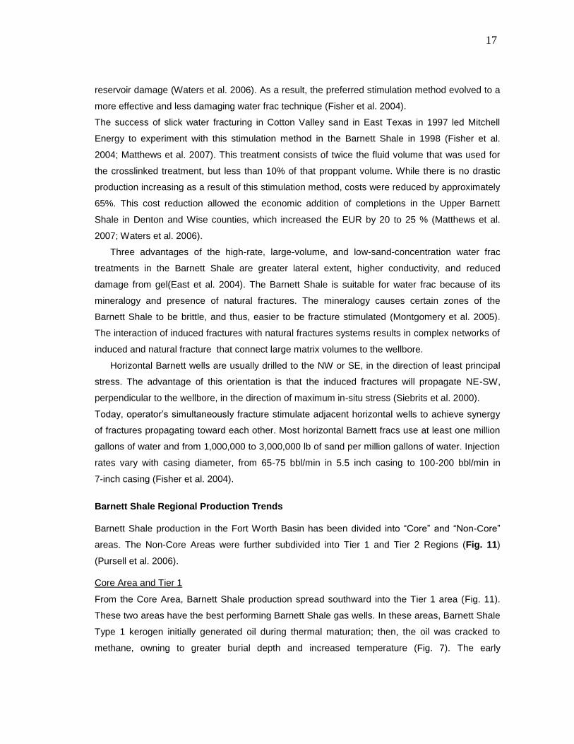
Barnett Shale production in the Fort Worth Basin has been divided into “Core” and “Non-Core”
areas. The Non-Core Areas were further subdivided into Tier 1 and Tier 2 Regions (Fig. 11)
(Pursell et al. 2006).
Core Area and Tier 1
From the Core Area, Barnett Shale production spread southward into the Tier 1 area (Fig. 11).
These two areas have the best performing Barnett Shale gas wells. In these areas, Barnett Shale
Type 1 kerogen initially generated oil during thermal maturation; then, the oil was cracked to
methane, owning to greater burial depth and increased temperature (Fig. 7). The early
18
development in the core area was most commonly with vertical wells completed with large
hydraulic fracture treatments. The presence of Viola Limestone frac barrier, which separates the
Barnett Shale from the underlying water-bearing Ellenberger Group (Figs. 3 and 4), made
possible large-scale fracture stimulation treatments in this region.
Tier 2
Tier 2 is divided into south and west areas (Fig. 11). The Viola Limestone fracture barrier (Fig. 3)
is absent in both areas, and thus, water production from the Ellenburger is a concern. Much of the
Barnett Shale in Tier 2 West is likely to produce oil rather than gas, based on the low thermal
maturity of the Barnett in this area (Figs. 7 and 11).
Barnett Oil Play
Barnett Shale production has expanded to the north and west of the Core Area (Fig. 11). Rather
than gas, however, the northern area produces oil, owing to the lower thermal maturity of the
Barnett Shale (Fig. 7) (EOG Resources 2008).
DALLAS
NAVARRO
ELLIS
COLLINYOUNG
STEPHENS
EASTLAND
ERATH
ARCHER
DENTON
WISE
PARKER TARRANT
BOSQUE
PALO PINTO
JACK
HILL
SOMERVELL
GRASON
ROCK
WALL
KAUFMAN
TIER 2
WEST
CORE
AREA
TIER 2
SOUTH
35 Miles
TIER 1
OIL
ZONE
COMANCHE
CLAY MONTAGUE COOKE
HOOD
N
DALLAS
NAVARRO
ELLIS
COLLINYOUNG
STEPHENS
EASTLAND
ERATH
ARCHER
DENTON
WISE
PARKER TARRANT
BOSQUE
PALO PINTO
JACK
HILL
SOMERVELL
GRASON
ROCK
WALL
KAUFMAN
TIER 2
WEST
CORE
AREA
TIER 2
SOUTH
35 Miles
TIER 1
OIL
ZONE
COMANCHE
CLAY MONTAGUE COOKE
HOOD
DALLAS
NAVARRO
ELLIS
COLLINYOUNG
STEPHENS
EASTLAND
ERATH
ARCHER
DENTON
WISE
PARKER TARRANT
BOSQUE
PALO PINTO
JACK
HILL
SOMERVELL
GRASON
ROCK
WALL
KAUFMAN
TIER 2
WEST
CORE
AREA
TIER 2
SOUTH
35 Miles
TIER 1
OIL
ZONE
COMANCHE
CLAY MONTAGUE COOKE
HOOD
N
Fig. 11–Barnett Shale well locations (HPDI 2008) and producing areas. Producing area outlines from (Pursell et al. 2006).
19
3. STRATIGRAPHIC ANALYSIS
Methodology
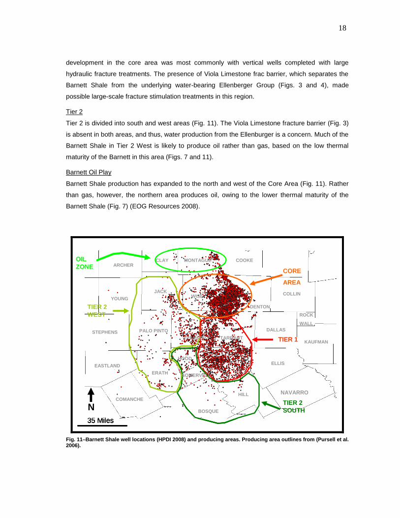
The Barnett Shale is a heterogeneous formation composed of numerous sedimentary sequences
that vary in thickness and, in a few cases, pinch out across the Fort Worth Basin. Some
sequences are shale- (clay-) rich, whereas others are dominated by carbonate or silty, siliceous
strata (Fig. 12). Mineralogy of the Barnett sequences affects mechanical properties, fracture
stimulation effectiveness, and production rates (Gale et al. 2007).
Fig. 12–Type well log showing Barnett Shale stratigraphy and reservoir units mapped in this study. See Fig. 13 for location.
20
Thus, decisions concerning where to perforate and stimulate require understanding lithology,
extent and thickness of the sedimentary sequences. To establish the distribution and thickness of
various lithologic units in the Barnett Shale, I used geophysical well logs to correlate the strata
and make structural and isopach maps. The stratigraphic framework constructed in this phase of
the study provided a basis for (1) assessing controls on Barnett Shale gas production (Section 4)
and (2) determining lithology of the various Barnett Shale intervals in a petrophysical study
(Section 5).
Approximately 800 depth-registered image well logs were used to analyze the structural and
stratigraphic settings of the Barnett Shale and adjacent formations (Fig. 12). The well logs used in
the study were selected on the basis of several criteria. First, we only used only vertical wells to
allow calculation of the interval thickness of units by subtracting depth of top of the interval from
depth of the base. Second, we selected only wells that penetrated the Barnett Shale. Third, we
only included only wells with porosity well logs, because porosity data were needed for
quantitative analysis. Fourth, we tried to optimize coverage of the basin. Based on those criteria,
we selected approximately 800 of 2,400 wells received from MS Systems. Well density is the
greatest in the core area of the eastern part of the basin.
Before assessing the vertical and lateral variability of Barnett Shale and evaluating reservoir
properties such as total organic carbon, we identified its top and base. Also, we identified and
correlated the Ellenburger top, Simpson Group, Viola Limestone, Chappel Limestone, Forestburg
Limestone, and base of the Marble Falls Limestone. We made structure maps for the Barnett
Shale and Forestburg Limestone to assess the primary structural features, and we mapped
thicknesses of the Barnett Shale and the Forestburg Ls.
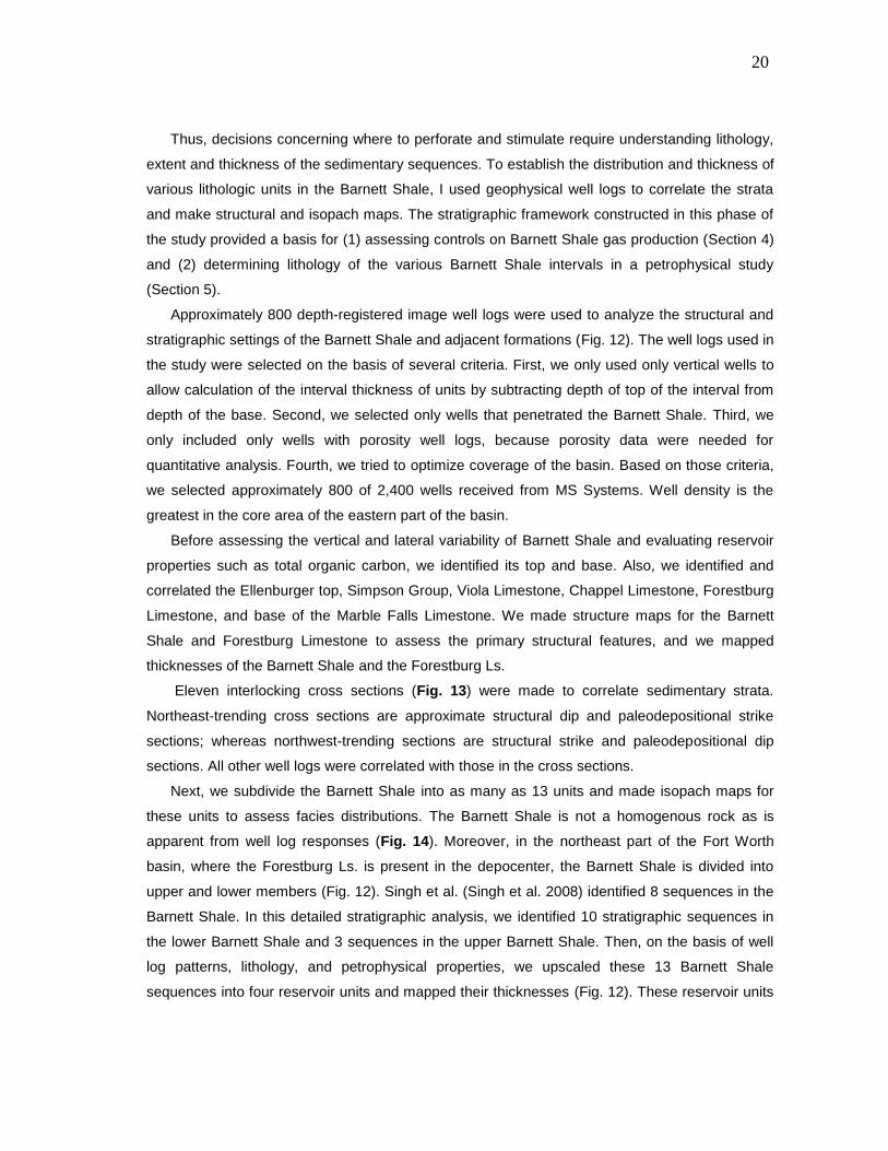
Eleven interlocking cross sections (Fig. 13) were made to correlate sedimentary strata.
Northeast-trending cross sections are approximate structural dip and paleodepositional strike
sections; whereas northwest-trending sections are structural strike and paleodepositional dip
sections. All other well logs were correlated with those in the cross sections.
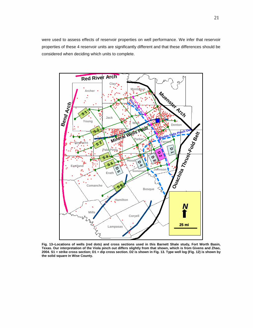
Next, we subdivide the Barnett Shale into as many as 13 units and made isopach maps for
these units to assess facies distributions. The Barnett Shale is not a homogenous rock as is
apparent from well log responses (Fig. 14). Moreover, in the northeast part of the Fort Worth
basin, where the Forestburg Ls. is present in the depocenter, the Barnett Shale is divided into
upper and lower members (Fig. 12). Singh et al. (Singh et al. 2008) identified 8 sequences in the
Barnett Shale. In this detailed stratigraphic analysis, we identified 10 stratigraphic sequences in
the lower Barnett Shale and 3 sequences in the upper Barnett Shale. Then, on the basis of well
log patterns, lithology, and petrophysical properties, we upscaled these 13 Barnett Shale
sequences into four reservoir units and mapped their thicknesses (Fig. 12). These reservoir units
21
were used to assess effects of reservoir properties on well performance. We infer that reservoir
properties of these 4 reservoir units are significantly different and that these differences should be
considered when deciding which units to complete.
NN
25 mi
S 1
S 6
S 5
S 4
S 3
S 2
D 3
D 2
D 5
D 4
D 1
Marble Falls Pinch Out
Viola P
inch Out
DentonWise
Tarrant
Johnson
Montague
Parker
Palo Pinto
Jack
Hood
Erath
Eastland
Clay
Comanche
Coryell
Bosque
Young
Stephens
Hamilton
Somervell
Lampasas
Mills
Archer
Ou
ach
ita T
hru
st-
Fo
ld B
elt
Ben
d A
rch
Muenster A
rch
Mineral Wells Fault
Red River Arch
NN
25 mi
NN
25 mi
NN
25 mi
S 1
S 6
S 5
S 4
S 3
S 2
D 3
D 2
D 5
D 4
D 1
Marble Falls Pinch Out
Viola P
inch Out
DentonWise
Tarrant
Johnson
Montague
Parker
Palo Pinto
Jack
Hood
Erath
Eastland
Clay
Comanche
Coryell
Bosque
Young
Stephens
Hamilton
Somervell
Lampasas
Mills
Archer
Ou
ach
ita T
hru
st-
Fo
ld B
elt
Ben
d A
rch
Muenster A
rch
Mineral Wells Fault
Red River Arch
Fig. 13–Locations of wells (red dots) and cross sections used in this Barnett Shale study, Fort Worth Basin, Texas. Our interpretation of the Viola pinch out differs slightly from that shown, which is from Givens and Zhao, 2004. S1 = strike cross section; D1 = dip cross section. D2 is shown in Fig. 13. Type well log (Fig. 12) is shown by the solid square in Wise County.
22
Fig. 14–Stratigraphic cross section showing the depositional center of the basin and identified Barnett Units 1-4.
23
Analysis of Barnett Shale Structure and Stratigraphy
Structural Features
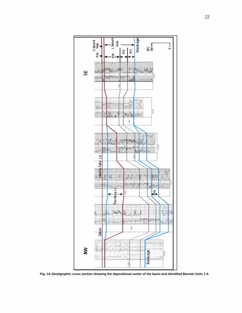
The Barnett Shale deepens northeastward from approximately -1,000 ft subsea level in Mills
County to -7,500 ft subsea level in central Denton County (Fig. 15) near the Muenster and
Ouachita Thrust Belt.
Fig. 15.–Structure, top of the Barnett Shale. Values are subsea level.
24
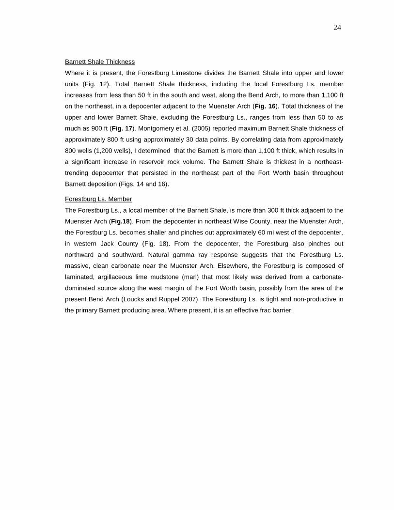
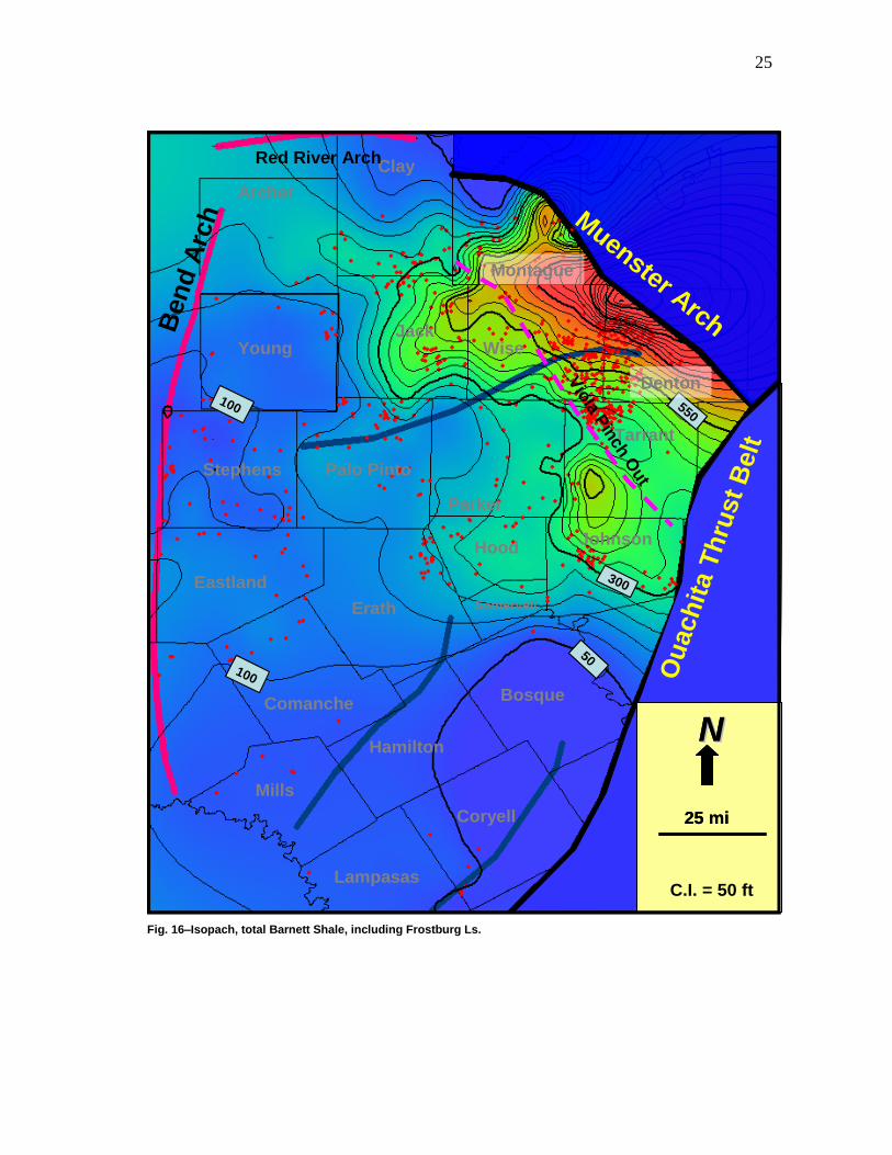
Barnett Shale Thickness
Where it is present, the Forestburg Limestone divides the Barnett Shale into upper and lower
units (Fig. 12). Total Barnett Shale thickness, including the local Forestburg Ls. member
increases from less than 50 ft in the south and west, along the Bend Arch, to more than 1,100 ft
on the northeast, in a depocenter adjacent to the Muenster Arch (Fig. 16). Total thickness of the
upper and lower Barnett Shale, excluding the Forestburg Ls., ranges from less than 50 to as
much as 900 ft (Fig. 17). Montgomery et al. (2005) reported maximum Barnett Shale thickness of
approximately 800 ft using approximately 30 data points. By correlating data from approximately
800 wells (1,200 wells), I determined that the Barnett is more than 1,100 ft thick, which results in
a significant increase in reservoir rock volume. The Barnett Shale is thickest in a northeast-
trending depocenter that persisted in the northeast part of the Fort Worth basin throughout
Barnett deposition (Figs. 14 and 16).
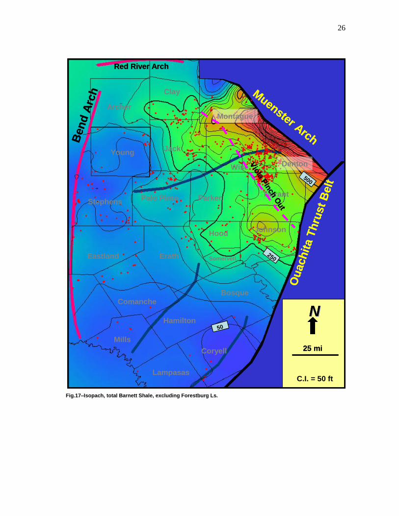
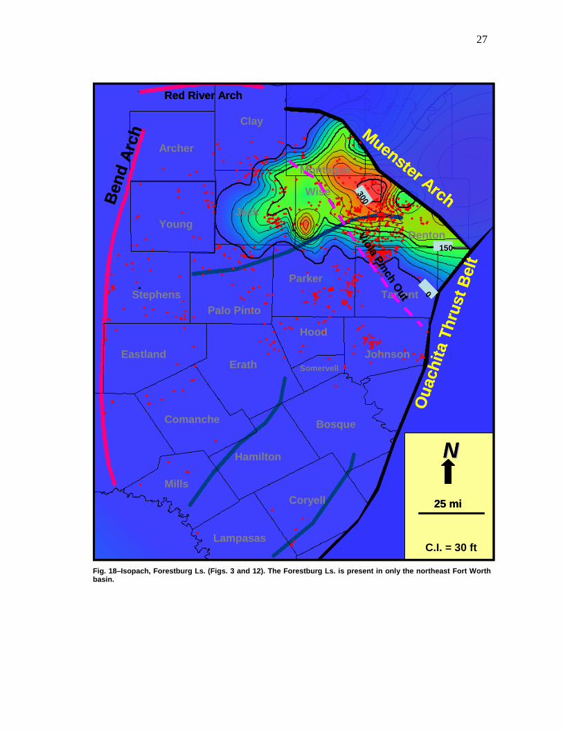
Forestburg Ls. Member
The Forestburg Ls., a local member of the Barnett Shale, is more than 300 ft thick adjacent to the
Muenster Arch (Fig.18). From the depocenter in northeast Wise County, near the Muenster Arch,
the Forestburg Ls. becomes shalier and pinches out approximately 60 mi west of the depocenter,
in western Jack County (Fig. 18). From the depocenter, the Forestburg also pinches out
northward and southward. Natural gamma ray response suggests that the Forestburg Ls.
massive, clean carbonate near the Muenster Arch. Elsewhere, the Forestburg is composed of
laminated, argillaceous lime mudstone (marl) that most likely was derived from a carbonate-
dominated source along the west margin of the Fort Worth basin, possibly from the area of the
present Bend Arch (Loucks and Ruppel 2007). The Forestburg Ls. is tight and non-productive in
the primary Barnett producing area. Where present, it is an effective frac barrier.
25
550
300
50
NN
25 mi
C.I. = 50 ft
100
100
Denton
Wise
Tarrant
Johnson
Montague
Parker
Palo Pinto
Jack
Hood
Erath
Eastland
Clay
Comanche
Coryell
Bosque
Young
Stephens
Hamilton
Somervell
Lampasas
Mills
Archer
Muenster Arch
Ou
ach
ita T
hru
st
Belt
Ben
d A
rch
Vio
la Pin
ch O
ut
Red River Arch
550
300
50
NN
25 mi
C.I. = 50 ft
100
100
Denton
Wise
Tarrant
Johnson
Montague
Parker
Palo Pinto
Jack
Hood
Erath
Eastland
Clay
Comanche
Coryell
Bosque
Young
Stephens
Hamilton
Somervell
Lampasas
Mills
Archer
550550
300300
5050
NN
25 mi
C.I. = 50 ft
NN
25 mi
NN
25 mi
C.I. = 50 ft
100100
100100
Denton
Wise
Tarrant
Johnson
Montague
Parker
Palo Pinto
Jack
Hood
Erath
Eastland
Clay
Comanche
Coryell
Bosque
Young
Stephens
Hamilton
Somervell
Lampasas
Mills
Archer
Muenster Arch
Ou
ach
ita T
hru
st
Belt
Ben
d A
rch
Vio
la Pin
ch O
ut
Red River Arch
Fig. 16–Isopach, total Barnett Shale, including Frostburg Ls.
26
500
250
50
NN
25 mi
C.I. = 50 ft
DentonWise
Tarrant
Johnson
Montague
ParkerPalo Pinto
Jack
Hood
ErathEastland
Clay
Comanche
Coryell
Bosque
Young
Stephens
Hamilton
Somervell
Lampasas
Mills
Archer
Muenster Arch
Ou
ach
ita T
hru
st
Belt
Ben
d A
rch
Vio
la Pin
ch O
ut
Red River Arch
500
250
50
NN
25 mi
C.I. = 50 ft
DentonWise
Tarrant
Johnson
Montague
ParkerPalo Pinto
Jack
Hood
ErathEastland
Clay
Comanche
Coryell
Bosque
Young
Stephens
Hamilton
Somervell
Lampasas
Mills
Archer
500
250
50
NN
25 mi
C.I. = 50 ft
500
250
50
NN
25 mi
C.I. = 50 ft
500500
250250
5050
NN
25 mi
C.I. = 50 ft
NN
25 mi
NN
25 mi
C.I. = 50 ft
DentonWise
Tarrant
Johnson
Montague
ParkerPalo Pinto
Jack
Hood
ErathEastland
Clay
Comanche
Coryell
Bosque
Young
Stephens
Hamilton
Somervell
Lampasas
Mills
Archer
Muenster Arch
Ou
ach
ita T
hru
st
Belt
Ben
d A
rch
Vio
la Pin
ch O
ut
Red River Arch
Muenster Arch
Ou
ach
ita T
hru
st
Belt
Ben
d A
rch
Vio
la Pin
ch O
ut
Red River Arch
Fig.17–Isopach, total Barnett Shale, excluding Forestburg Ls.
27
0
150
300
NN
25 mi
C.I. = 30 ft
Denton
Wise
Tarrant
Johnson
Montague
Parker
Palo Pinto
Jack
Hood
ErathEastland
Clay
Comanche
Coryell
Bosque
Young
Stephens
Hamilton
Somervell
Lampasas
Mills
Archer
Muenster Arch
Ou
ach
ita T
hru
st
Belt
Ben
d A
rch
Vio
la Pin
ch O
ut
Red River Arch
0
150
300
NN
25 mi
C.I. = 30 ft
Denton
Wise
Tarrant
Johnson
Montague
Parker
Palo Pinto
Jack
Hood
ErathEastland
Clay
Comanche
Coryell
Bosque
Young
Stephens
Hamilton
Somervell
Lampasas
Mills
Archer
0
150
300
NN
25 mi
C.I. = 30 ft
0
150
300
NN
25 mi
C.I. = 30 ft
0
150
300
00
150150
300 300
NN
25 mi
C.I. = 30 ft
NN
25 mi
NN
25 mi
C.I. = 30 ft
Denton
Wise
Tarrant
Johnson
Montague
Parker
Palo Pinto
Jack
Hood
ErathEastland
Clay
Comanche
Coryell
Bosque
Young
Stephens
Hamilton
Somervell
Lampasas
Mills
Archer
Muenster Arch
Ou
ach
ita T
hru
st
Belt
Ben
d A
rch
Vio
la Pin
ch O
ut
Red River Arch
Muenster Arch
Ou
ach
ita T
hru
st
Belt
Ben
d A
rch
Vio
la Pin
ch O
ut
Red River Arch
Fig. 18–Isopach, Forestburg Ls. (Figs. 3 and 12). The Forestburg Ls. is present in only the northeast Fort Worth basin.
28
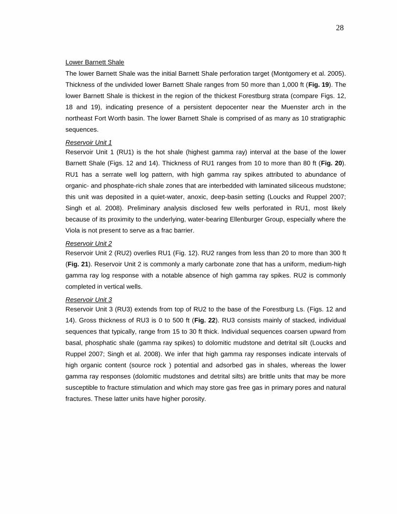
Lower Barnett Shale
The lower Barnett Shale was the initial Barnett Shale perforation target (Montgomery et al. 2005).
Thickness of the undivided lower Barnett Shale ranges from 50 more than 1,000 ft (Fig. 19). The
lower Barnett Shale is thickest in the region of the thickest Forestburg strata (compare Figs. 12,
18 and 19), indicating presence of a persistent depocenter near the Muenster arch in the
northeast Fort Worth basin. The lower Barnett Shale is comprised of as many as 10 stratigraphic
sequences.
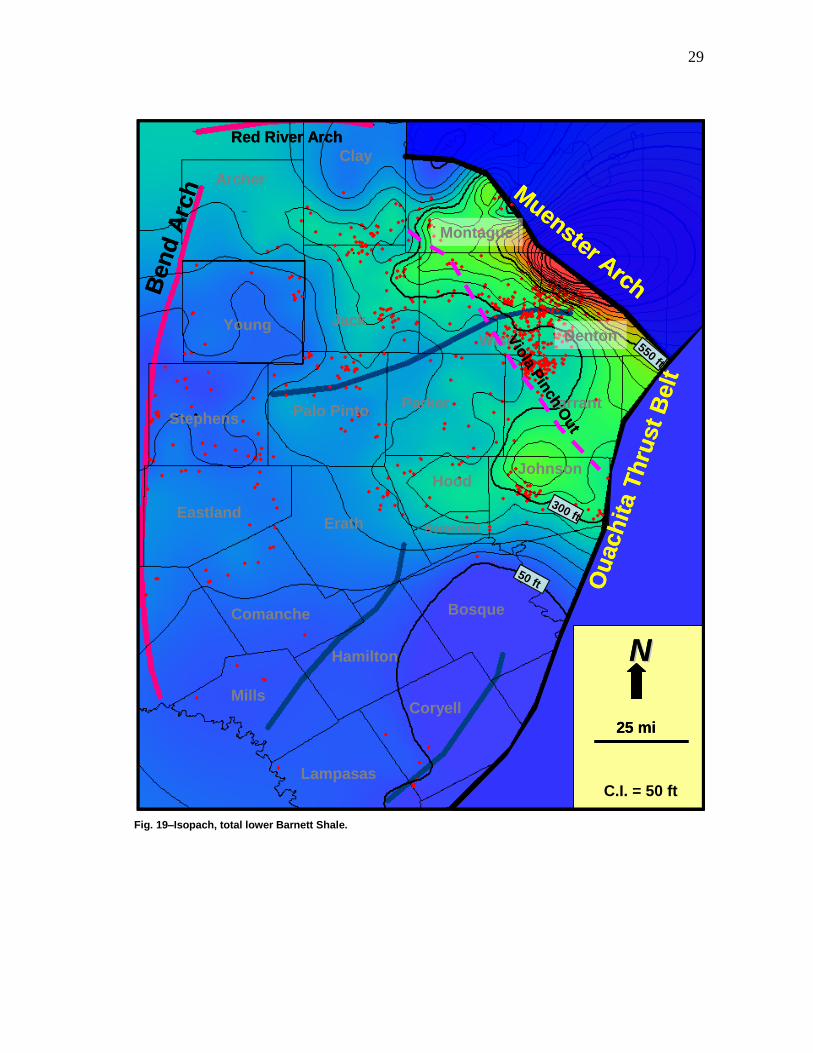
Reservoir Unit 1
Reservoir Unit 1 (RU1) is the hot shale (highest gamma ray) interval at the base of the lower
Barnett Shale (Figs. 12 and 14). Thickness of RU1 ranges from 10 to more than 80 ft (Fig. 20).
RU1 has a serrate well log pattern, with high gamma ray spikes attributed to abundance of
organic- and phosphate-rich shale zones that are interbedded with laminated siliceous mudstone;
this unit was deposited in a quiet-water, anoxic, deep-basin setting (Loucks and Ruppel 2007;
Singh et al. 2008). Preliminary analysis disclosed few wells perforated in RU1, most likely
because of its proximity to the underlying, water-bearing Ellenburger Group, especially where the
Viola is not present to serve as a frac barrier.
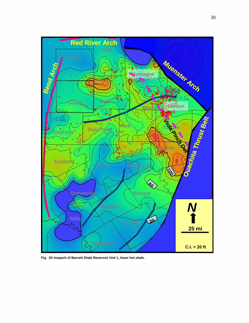
Reservoir Unit 2
Reservoir Unit 2 (RU2) overlies RU1 (Fig. 12). RU2 ranges from less than 20 to more than 300 ft
(Fig. 21). Reservoir Unit 2 is commonly a marly carbonate zone that has a uniform, medium-high
gamma ray log response with a notable absence of high gamma ray spikes. RU2 is commonly
completed in vertical wells.
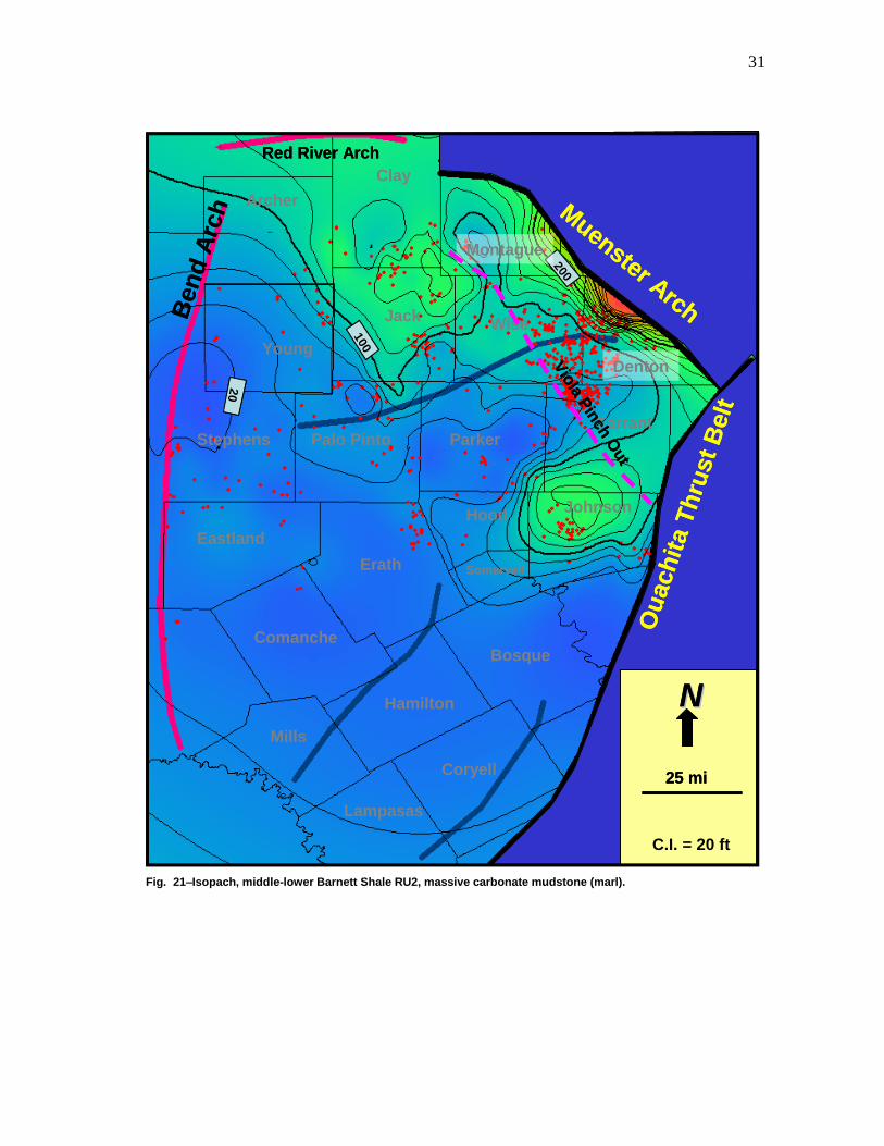
Reservoir Unit 3
Reservoir Unit 3 (RU3) extends from top of RU2 to the base of the Forestburg Ls. (Figs. 12 and
14). Gross thickness of RU3 is 0 to 500 ft (Fig. 22). RU3 consists mainly of stacked, individual
sequences that typically, range from 15 to 30 ft thick. Individual sequences coarsen upward from
basal, phosphatic shale (gamma ray spikes) to dolomitic mudstone and detrital silt (Loucks and
Ruppel 2007; Singh et al. 2008). We infer that high gamma ray responses indicate intervals of
high organic content (source rock ) potential and adsorbed gas in shales, whereas the lower
gamma ray responses (dolomitic mudstones and detrital silts) are brittle units that may be more
susceptible to fracture stimulation and which may store gas free gas in primary pores and natural
fractures. These latter units have higher porosity.
29
550 ft
300 ft
50 ft
NN
25 mi
C.I. = 50 ft
DentonWise
Tarrant
Johnson
Montague
ParkerPalo Pinto
Jack
Hood
ErathEastland
Clay
Comanche
Coryell
Bosque
Young
Stephens
Hamilton
Somervell
Lampasas
Mills
ArcherM
uenster Arch
Ou
ach
ita T
hru
st
Belt
Ben
d A
rch
Vio
la Pin
ch O
ut
Red River Arch
550 ft
300 ft
50 ft
NN
25 mi
C.I. = 50 ft
DentonWise
Tarrant
Johnson
Montague
ParkerPalo Pinto
Jack
Hood
ErathEastland
Clay
Comanche
Coryell
Bosque
Young
Stephens
Hamilton
Somervell
Lampasas
Mills
Archer
550 ft
300 ft
50 ft
NN
25 mi
C.I. = 50 ft
550 ft
300 ft
50 ft
NN
25 mi
C.I. = 50 ft
550 ft
300 ft
50 ft
550 ft
550 ft
300 ft300 ft
50 ft50 ft
NN
25 mi
C.I. = 50 ft
NN
25 mi
NN
25 mi
C.I. = 50 ft
DentonWise
Tarrant
Johnson
Montague
ParkerPalo Pinto
Jack
Hood
ErathEastland
Clay
Comanche
Coryell
Bosque
Young
Stephens
Hamilton
Somervell
Lampasas
Mills
ArcherM
uenster Arch
Ou
ach
ita T
hru
st
Belt
Ben
d A
rch
Vio
la Pin
ch O
ut
Red River Arch
Muenster Arch
Ou
ach
ita T
hru
st
Belt
Ben
d A
rch
Vio
la Pin
ch O
ut
Red River Arch
Fig. 19–Isopach, total lower Barnett Shale.
30
60
100
20
DentonWise
Tarrant
Johnson
Montague
Park
erPalo Pinto
Jack
Hood
ErathEastland
Clay
Comanche
Coryell
Bosque
Young
Stephens
Hamilton
Somervell
Lampasas
Mills
Archer
NN
25 mi
C.I. = 20 ft
Muenster Arch
Ou
ach
ita T
hru
st
Belt
Ben
d A
rch
Vio
la Pin
ch O
ut
Red River Arch
60
100
20
DentonWise
Tarrant
Johnson
Montague
Park
erPalo Pinto
Jack
Hood
ErathEastland
Clay
Comanche
Coryell
Bosque
Young
Stephens
Hamilton
Somervell
Lampasas
Mills
Archer
NN
25 mi
C.I. = 20 ft
6060
100
2020
DentonWise
Tarrant
Johnson
Montague
Park
erPalo Pinto
Jack
Hood
ErathEastland
Clay
Comanche
Coryell
Bosque
Young
Stephens
Hamilton
Somervell
Lampasas
Mills
Archer
NN
25 mi
C.I. = 20 ft
Muenster Arch
Ou
ach
ita T
hru
st
Belt
Ben
d A
rch
Vio
la Pin
ch O
ut
Red River Arch
Muenster Arch
Ou
ach
ita T
hru
st
Belt
Ben
d A
rch
Vio
la Pin
ch O
ut
Red River Arch
Fig. 20–Isopach of Barnett Shale Reservoir Unit 1, lower hot shale.
31
NN
25 mi
C.I. = 20 ft
200
100
20
Denton
Wise
Tarrant
Johnson
Montague
ParkerPalo Pinto
Jack
Hood
Erath
Eastland
Clay
Comanche
Coryell
Bosque
Young
Stephens
Hamilton
Somervell
Lampasas
Mills
Archer Muenster Arch
Ou
ach
ita T
hru
st
Belt
Ben
d A
rch
Vio
la Pin
ch O
ut
Red River Arch
NN
25 mi
C.I. = 20 ft
NN
25 mi
NN
25 mi
C.I. = 20 ft
200200
100
100
20
20
Denton
Wise
Tarrant
Johnson
Montague
ParkerPalo Pinto
Jack
Hood
Erath
Eastland
Clay
Comanche
Coryell
Bosque
Young
Stephens
Hamilton
Somervell
Lampasas
Mills
Archer Muenster Arch
Ou
ach
ita T
hru
st
Belt
Ben
d A
rch
Vio
la Pin
ch O
ut
Red River Arch
Muenster Arch
Ou
ach
ita T
hru
st
Belt
Ben
d A
rch
Vio
la Pin
ch O
ut
Red River Arch
Fig. 21–Isopach, middle-lower Barnett Shale RU2, massive carbonate mudstone (marl).

32
NN
25 mi
C.I. = 20 ft
200
100
20
Denton
Wise
Tarrant
Johnson
Montague
ParkerPalo Pinto
Jack
Hood
Erath
Eastland
Clay
Comanche
Coryell
Bosque
Young
Stephens
Hamilton
Somervell
Lampasas
Mills
Archer Muenster Arch
Ou
ach
ita T
hru
st
Belt
Ben
d A
rch
Vio
la Pin
ch O
ut
Red River Arch
NN
25 mi
C.I. = 20 ft
NN
25 mi
NN
25 mi
C.I. = 20 ft
200200
100
100
20
20
Denton
Wise
Tarrant
Johnson
Montague
ParkerPalo Pinto
Jack
Hood
Erath
Eastland
Clay
Comanche
Coryell
Bosque
Young
Stephens
Hamilton
Somervell
Lampasas
Mills
Archer Muenster Arch
Ou
ach
ita T
hru
st
Belt
Ben
d A
rch
Vio
la Pin
ch O
ut
Red River Arch
Muenster Arch
Ou
ach
ita T
hru
st
Belt
Ben
d A
rch
Vio
la Pin
ch O
ut
Red River Arch
Fig. 22–Isopach, lower Barnett Shale RU3 (upper lower Barnett), mainly upward-coarsening sequences (Fig. 2). Most wells are completed in this interval.
33
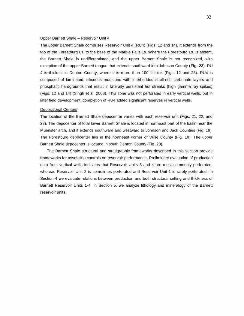
Upper Barnett Shale – Reservoir Unit 4
The upper Barnett Shale comprises Reservoir Unit 4 (RU4) (Figs. 12 and 14). It extends from the
top of the Forestburg Ls. to the base of the Marble Falls Ls. Where the Forestburg Ls. is absent,
the Barnett Shale is undifferentiated, and the upper Barnett Shale is not recognized, with
exception of the upper Barnett tongue that extends southward into Johnson County (Fig. 23). RU
4 is thickest in Denton County, where it is more than 100 ft thick (Figs. 12 and 23). RU4 is
composed of laminated, siliceous mudstone with interbedded shell-rich carbonate layers and
phosphatic hardgrounds that result in laterally persistent hot streaks (high gamma ray spikes)
(Figs. 12 and 14) (Singh et al. 2008). This zone was not perforated in early vertical wells, but in
later field development, completion of RU4 added significant reserves in vertical wells.
Depositional Centers
The location of the Barnett Shale depocenter varies with each reservoir unit (Figs. 21, 22, and
23). The depocenter of total lower Barnett Shale is located in northeast part of the basin near the
Muenster arch, and it extends southward and westward to Johnson and Jack Counties (Fig. 19).
The Forestburg depocenter lies in the northeast corner of Wise County (Fig. 18). The upper
Barnett Shale depocenter is located in south Denton County (Fig. 23).
The Barnett Shale structural and stratigraphic frameworks described in this section provide
frameworks for assessing controls on reservoir performance. Preliminary evaluation of production
data from vertical wells indicates that Reservoir Units 3 and 4 are most commonly perforated,
whereas Reservoir Unit 2 is sometimes perforated and Reservoir Unit 1 is rarely perforated. In
Section 4 we evaluate relations between production and both structural setting and thickness of
Barnett Reservoir Units 1-4. In Section 5, we analyze lithology and mineralogy of the Barnett
reservoir units.
34
NN
25 mi
C.I. = 10 ft
100
50
0
DentonWise
Tarrant
Johnson
Montague
ParkerPalo Pinto
Jack
Hood
ErathEastland
Clay
Comanche
Coryell
Bosque
Young
Stephens
Hamilton
Somervell
Lampasas
Mills
Archer
Muenster Arch
Ou
ach
ita T
hru
st
Belt
Ben
d A
rch
Vio
la Pin
ch O
ut
Red River Arch
NN
25 mi
C.I. = 20 ft
NN
25 mi
C.I. = 10 ft
100
50
0
DentonWise
Tarrant
Johnson
Montague
ParkerPalo Pinto
Jack
Hood
ErathEastland
Clay
Comanche
Coryell
Bosque
Young
Stephens
Hamilton
Somervell
Lampasas
Mills
Archer
Muenster Arch
Ou
ach
ita T
hru
st
Belt
Ben
d A
rch
Vio
la Pin
ch O
ut
Red River Arch
NN
25 mi
C.I. = 10 ft
100
50
0
DentonWise
Tarrant
Johnson
Montague
ParkerPalo Pinto
Jack
Hood
ErathEastland
Clay
Comanche
Coryell
Bosque
Young
Stephens
Hamilton
Somervell
Lampasas
Mills
Archer
NN
25 mi
C.I. = 10 ft
100
50
0
NN
25 mi
C.I. = 10 ft
100
50
0
NN
25 mi
NN
25 mi
C.I. = 10 ft
100100
50
0
DentonWise
Tarrant
Johnson
Montague
ParkerPalo Pinto
Jack
Hood
ErathEastland
Clay
Comanche
Coryell
Bosque
Young
Stephens
Hamilton
Somervell
Lampasas
Mills
Archer
Muenster Arch
Ou
ach
ita T
hru
st
Belt
Ben
d A
rch
Vio
la Pin
ch O
ut
Red River Arch
Muenster Arch
Ou
ach
ita T
hru
st
Belt
Ben
d A
rch
Vio
la Pin
ch O
ut
Red River Arch
NN
25 mi
C.I. = 20 ft
NN
25 mi
NN
25 mi
C.I. = 20 ft
Fig. 23–Isopach, upper Barnett Shale (RU4), which is recognizable where the Forestburg Ls. is present.
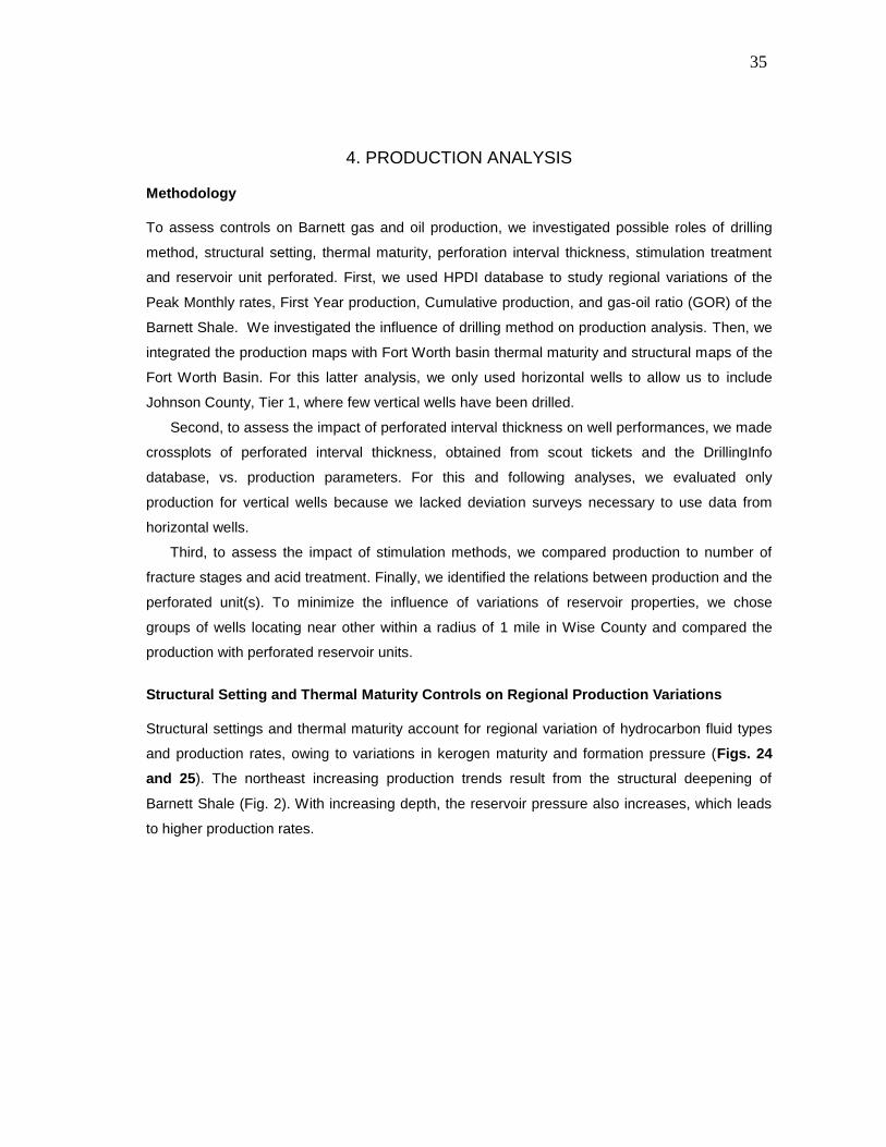
35
4. PRODUCTION ANALYSIS
Methodology
To assess controls on Barnett gas and oil production, we investigated possible roles of drilling
method, structural setting, thermal maturity, perforation interval thickness, stimulation treatment
and reservoir unit perforated. First, we used HPDI database to study regional variations of the
Peak Monthly rates, First Year production, Cumulative production, and gas-oil ratio (GOR) of the
Barnett Shale. We investigated the influence of drilling method on production analysis. Then, we
integrated the production maps with Fort Worth basin thermal maturity and structural maps of the
Fort Worth Basin. For this latter analysis, we only used horizontal wells to allow us to include
Johnson County, Tier 1, where few vertical wells have been drilled.
Second, to assess the impact of perforated interval thickness on well performances, we made
crossplots of perforated interval thickness, obtained from scout tickets and the DrillingInfo
database, vs. production parameters. For this and following analyses, we evaluated only
production for vertical wells because we lacked deviation surveys necessary to use data from
horizontal wells.
Third, to assess the impact of stimulation methods, we compared production to number of
fracture stages and acid treatment. Finally, we identified the relations between production and the
perforated unit(s). To minimize the influence of variations of reservoir properties, we chose
groups of wells locating near other within a radius of 1 mile in Wise County and compared the
production with perforated reservoir units.
Structural Setting and Thermal Maturity Controls on Regional Production Variations
Structural settings and thermal maturity account for regional variation of hydrocarbon fluid types
and production rates, owing to variations in kerogen maturity and formation pressure (Figs. 24
and 25). The northeast increasing production trends result from the structural deepening of
Barnett Shale (Fig. 2). With increasing depth, the reservoir pressure also increases, which leads
to higher production rates.
36
Fig. 24–Structure on the base of the Barnett Shale showing limits of the Viola and Marble Falls frac barriers (modified Givens and Zhao 2007), with overlay of Barnett Shale gas well locations (from HPDI 2008).
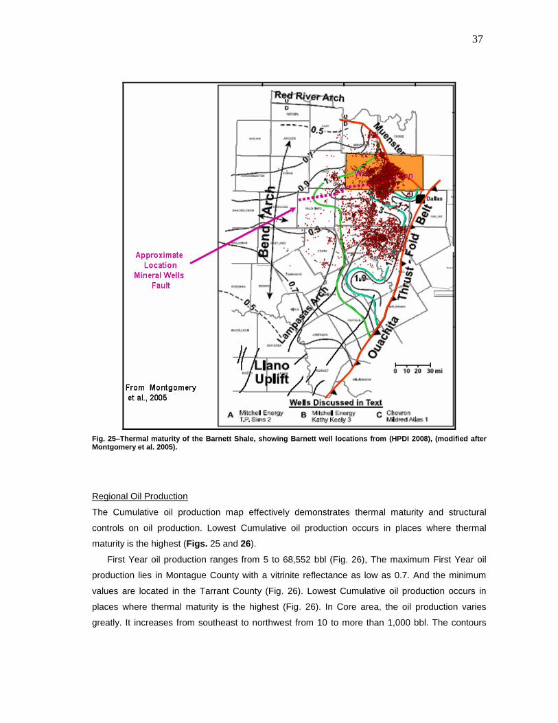
37
Fig. 25–Thermal maturity of the Barnett Shale, showing Barnett well locations from (HPDI 2008), (modified after Montgomery et al. 2005).
Regional Oil Production
The Cumulative oil production map effectively demonstrates thermal maturity and structural
controls on oil production. Lowest Cumulative oil production occurs in places where thermal
maturity is the highest (Figs. 25 and 26).
First Year oil production ranges from 5 to 68,552 bbl (Fig. 26), The maximum First Year oil
production lies in Montague County with a vitrinite reflectance as low as 0.7. And the minimum
values are located in the Tarrant County (Fig. 26). Lowest Cumulative oil production occurs in
places where thermal maturity is the highest (Fig. 26). In Core area, the oil production varies
greatly. It increases from southeast to northwest from 10 to more than 1,000 bbl. The contours
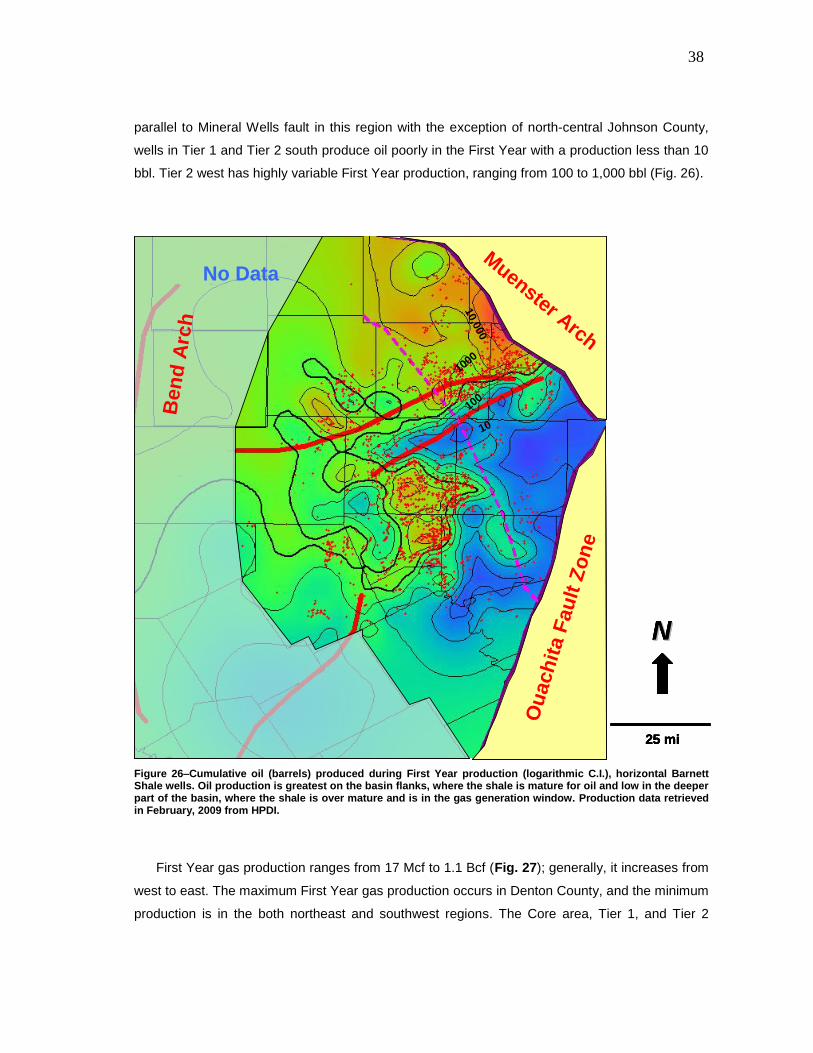
38
parallel to Mineral Wells fault in this region with the exception of north-central Johnson County,
wells in Tier 1 and Tier 2 south produce oil poorly in the First Year with a production less than 10
bbl. Tier 2 west has highly variable First Year production, ranging from 100 to 1,000 bbl (Fig. 26).
No Data
Ben
d A
rch
Muenster Arch
Ou
ach
ita F
au
lt Z
on
e
NN
25 mi
10
100
100010,0
00
No Data
Ben
d A
rch
Muenster Arch
Ou
ach
ita F
au
lt Z
on
e
NN
25 mi
No Data
Ben
d A
rch
Muenster Arch
Ou
ach
ita F
au
lt Z
on
e
NN
25 mi
NN
25 mi
10
100
100010,0
00
Figure 26–Cumulative oil (barrels) produced during First Year production (logarithmic C.I.), horizontal Barnett Shale wells. Oil production is greatest on the basin flanks, where the shale is mature for oil and low in the deeper part of the basin, where the shale is over mature and is in the gas generation window. Production data retrieved in February, 2009 from HPDI.
First Year gas production ranges from 17 Mcf to 1.1 Bcf (Fig. 27); generally, it increases from
west to east. The maximum First Year gas production occurs in Denton County, and the minimum
production is in the both northeast and southwest regions. The Core area, Tier 1, and Tier 2
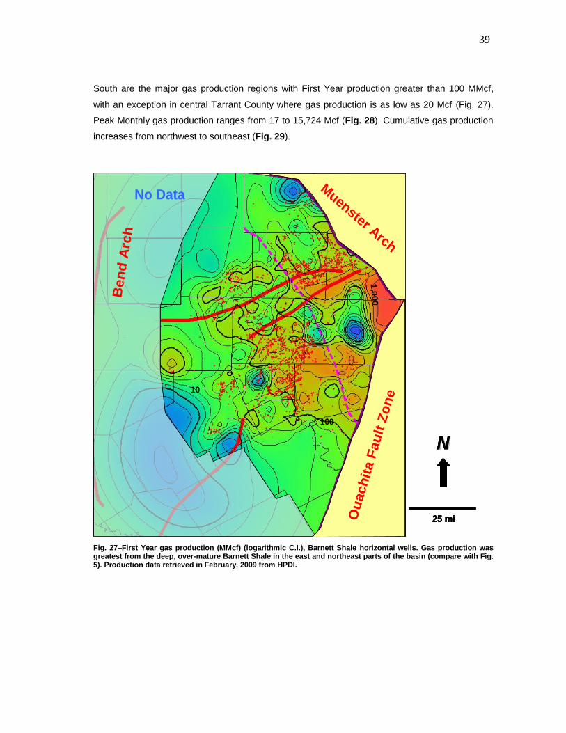
39
South are the major gas production regions with First Year production greater than 100 MMcf,
with an exception in central Tarrant County where gas production is as low as 20 Mcf (Fig. 27).
Peak Monthly gas production ranges from 17 to 15,724 Mcf (Fig. 28). Cumulative gas production
increases from northwest to southeast (Fig. 29).
No Data
Ben
d A
rch
Muenster Arch
Ou
ach
ita F
au
lt Z
on
e
NN
25 mi
100
10
1,0
00
No Data
Ben
d A
rch
Muenster Arch
Ou
ach
ita F
au
lt Z
on
e
NN
25 mi
No Data
Ben
d A
rch
Muenster Arch
Ou
ach
ita F
au
lt Z
on
e
NN
25 mi
NN
25 mi
100
10
1,0
00
Fig. 27–First Year gas production (MMcf) (logarithmic C.I.), Barnett Shale horizontal wells. Gas production was greatest from the deep, over-mature Barnett Shale in the east and northeast parts of the basin (compare with Fig. 5). Production data retrieved in February, 2009 from HPDI.
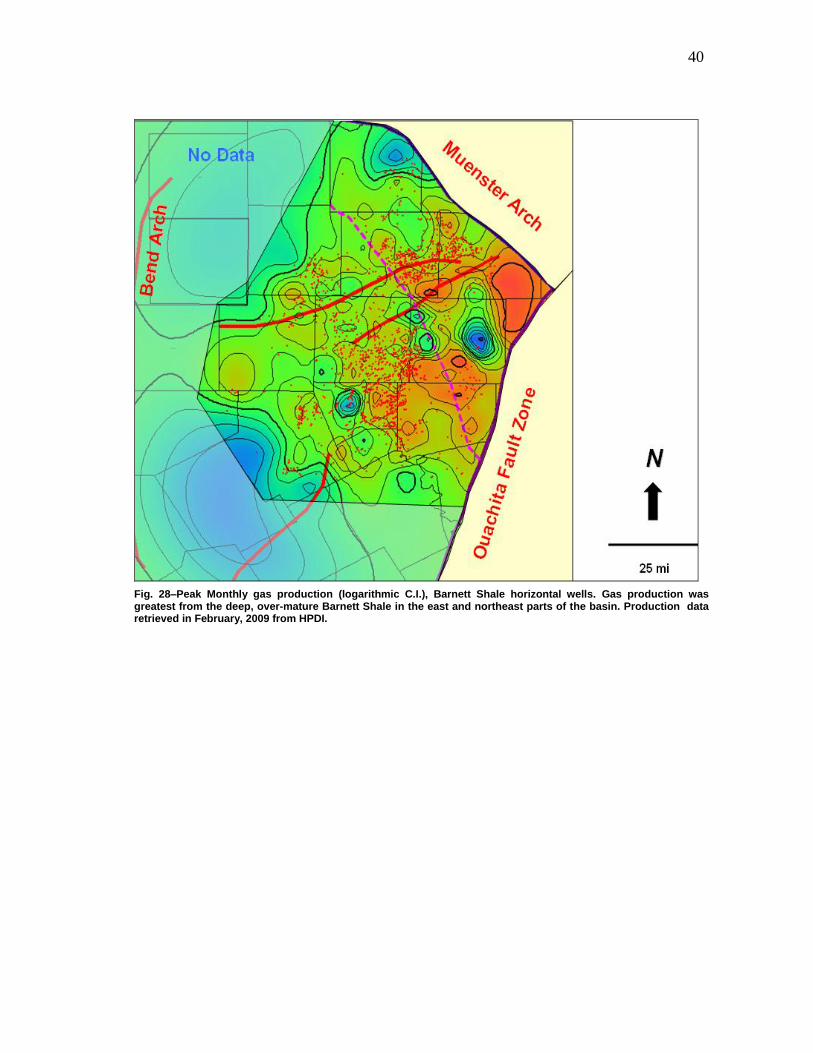
40
Fig. 28–Peak Monthly gas production (logarithmic C.I.), Barnett Shale horizontal wells. Gas production was greatest from the deep, over-mature Barnett Shale in the east and northeast parts of the basin. Production data retrieved in February, 2009 from HPDI.
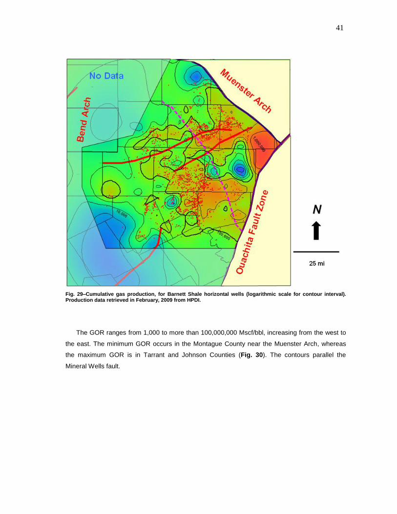
41
Fig. 29–Cumulative gas production, for Barnett Shale horizontal wells (logarithmic scale for contour interval). Production data retrieved in February, 2009 from HPDI.
The GOR ranges from 1,000 to more than 100,000,000 Mscf/bbl, increasing from the west to
the east. The minimum GOR occurs in the Montague County near the Muenster Arch, whereas
the maximum GOR is in Tarrant and Johnson Counties (Fig. 30). The contours parallel the
Mineral Wells fault.
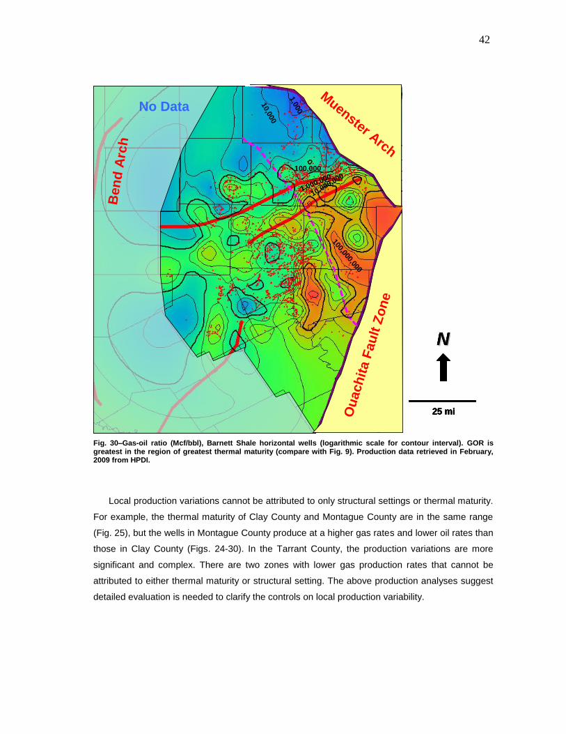
42
No DataB
en
d A
rch
Muenster Arch
Ou
ach
ita F
au
lt Z
on
e
NN
25 mi
100,000,000
10,000,000
1,000,000
100,000
10,0
00
1,0
00No Data
Ben
d A
rch
Muenster Arch
Ou
ach
ita F
au
lt Z
on
e
NN
25 mi
No DataB
en
d A
rch
Muenster Arch
Ou
ach
ita F
au
lt Z
on
e
NN
25 mi
NN
25 mi
100,000,000
10,000,000
1,000,000
100,000
10,0
00
1,0
00
Fig. 30–Gas-oil ratio (Mcf/bbl), Barnett Shale horizontal wells (logarithmic scale for contour interval). GOR is greatest in the region of greatest thermal maturity (compare with Fig. 9). Production data retrieved in February, 2009 from HPDI.
Local production variations cannot be attributed to only structural settings or thermal maturity.
For example, the thermal maturity of Clay County and Montague County are in the same range
(Fig. 25), but the wells in Montague County produce at a higher gas rates and lower oil rates than
those in Clay County (Figs. 24-30). In the Tarrant County, the production variations are more
significant and complex. There are two zones with lower gas production rates that cannot be
attributed to either thermal maturity or structural setting. The above production analyses suggest
detailed evaluation is needed to clarify the controls on local production variability.
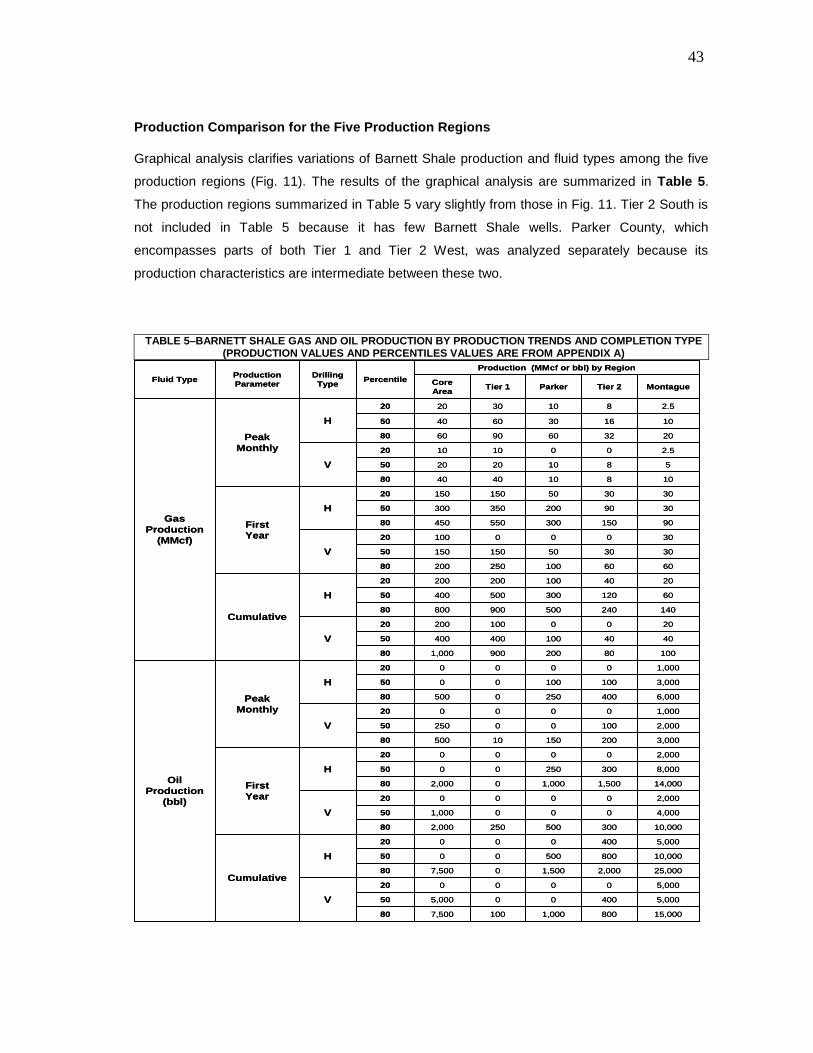
43
Production Comparison for the Five Production Regions
Graphical analysis clarifies variations of Barnett Shale production and fluid types among the five
production regions (Fig. 11). The results of the graphical analysis are summarized in Table 5.
The production regions summarized in Table 5 vary slightly from those in Fig. 11. Tier 2 South is
not included in Table 5 because it has few Barnett Shale wells. Parker County, which
encompasses parts of both Tier 1 and Tier 2 West, was analyzed separately because its
production characteristics are intermediate between these two.
TABLE 5–BARNETT SHALE GAS AND OIL PRODUCTION BY PRODUCTION TRENDS AND COMPLETION TYPE (PRODUCTION VALUES AND PERCENTILES VALUES ARE FROM APPENDIX A)
15,0008001,0001007,50080
5,000400005,00050
5,000000020
V
25,0002,0001,50007,50080
10,0008005000050
5,00040000020
H
Cumulative
10,0003005002502,00080
4,0000001,00050
2,000000020
V
14,0001,5001,00002,00080
8,0003002500050
2,000000020
H
First
Year
3,0002001501050080
2,0001000025050
1,000000020
V
6,000400250050080
3,0001001000050
1,000000020
H
Peak
Monthly
Oil
Production
(bbl)
100802009001,00080
404010040040050
200010020020
V
14024050090080080
6012030050040050
204010020020020
H
Cumulative
606010025020080
30305015015050
3000010020
V
9015030055045080
309020035030050
30305015015020
H
First
Year
10810404080
5810202050
2.500101020
V
203260906080
101630604050
2.5810302020
H
Peak
Monthly
Gas
Production
(MMcf)
MontagueTier 2ParkerTier 1Core
Area
Production (MMcf or bbl) by Region
PercentileDrilling
Type
Production
ParameterFluid Type
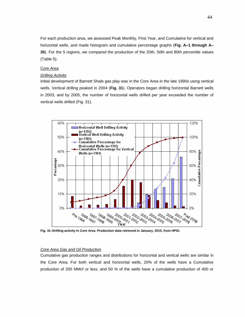
44
For each production area, we assessed Peak Monthly, First Year, and Cumulative for vertical and
horizontal wells, and made histogram and cumulative percentage graphs (Fig. A–1 through A–
30). For the 5 regions, we compared the production of the 20th, 50th and 80th percentile values
(Table 5).
Core Area
Drilling Activity
Initial development of Barnett Shale gas play was in the Core Area in the late 1990s using vertical
wells. Vertical drilling peaked in 2004 (Fig. 31). Operators began drilling horizontal Barnett wells
in 2003, and by 2005, the number of horizontal wells drilled per year exceeded the number of
vertical wells drilled (Fig. 31).
Fig. 31–Drilling activity in Core Area. Production data retrieved in January, 2010, from HPDI.
Core Area Gas and Oil Production
Cumulative gas production ranges and distributions for horizontal and vertical wells are similar in
the Core Area. For both vertical and horizontal wells, 20% of the wells have a Cumulative
production of 200 MMcf or less, and 50 % of the wells have a cumulative production of 400 or
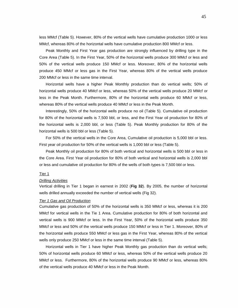
45
less MMcf (Table 5). However, 80% of the vertical wells have cumulative production 1000 or less
MMcf, whereas 80% of the horizontal wells have cumulative production 800 MMcf or less.
Peak Monthly and First Year gas production are strongly influenced by drilling type in the
Core Area (Table 5). In the First Year, 50% of the horizontal wells produce 300 MMcf or less and
50% of the vertical wells produce 150 MMcf or less. Moreover, 80% of the horizontal wells
produce 450 MMcf or less gas in the First Year, whereas 80% of the vertical wells produce
200 MMcf or less in the same time interval.
Horizontal wells have a higher Peak Monthly production than do vertical wells; 50% of
horizontal wells produce 40 MMcf or less, whereas 50% of the vertical wells produce 20 MMcf or
less in the Peak Month. Furthermore, 80% of the horizontal wells produce 60 MMcf or less,
whereas 80% of the vertical wells produce 40 MMcf or less in the Peak Month.
Interestingly, 50% of the horizontal wells produce no oil (Table 5). Cumulative oil production
for 80% of the horizontal wells is 7,500 bbl, or less, and the First Year oil production for 80% of
the horizontal wells is 2,000 bbl, or less (Table 5). Peak Monthly production for 80% of the
horizontal wells is 500 bbl or less (Table 5).
For 50% of the vertical wells in the Core Area, Cumulative oil production is 5,000 bbl or less.
First year oil production for 50% of the vertical wells is 1,000 bbl or less (Table 5).
Peak Monthly oil production for 80% of both vertical and horizontal wells is 500 bbl or less in
the Core Area. First Year oil production for 80% of both vertical and horizontal wells is 2,000 bbl
or less and cumulative oil production for 80% of the wells of both types is 7,500 bbl or less.
Tier 1
Drilling Activities
Vertical drilling in Tier 1 began in earnest in 2002 (Fig 32). By 2005, the number of horizontal
wells drilled annually exceeded the number of vertical wells (Fig 32).
Tier 1 Gas and Oil Production
Cumulative gas production of 50% of the horizontal wells is 350 MMcf or less, whereas it is 200
MMcf for vertical wells in the Tie 1 Area. Cumulative production for 80% of both horizontal and
vertical wells is 900 MMcf or less. In the First Year, 50% of the horizontal wells produce 350
MMcf or less and 50% of the vertical wells produce 150 MMcf or less in Tier 1. Moreover, 80% of
the horizontal wells produce 550 MMcf or less gas in the First Year, whereas 80% of the vertical
wells only produce 250 MMcf or less in the same time interval (Table 5).
Horizontal wells in Tier 1 have higher Peak Monthly gas production than do vertical wells;
50% of horizontal wells produce 60 MMcf or less, whereas 50% of the vertical wells produce 20
MMcf or less. Furthermore, 80% of the horizontal wells produce 90 MMcf or less, whereas 80%
of the vertical wells produce 40 MMcf or less in the Peak Month.
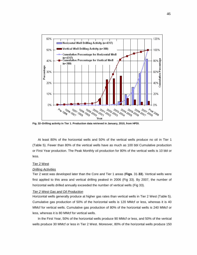
46
Fig. 32–Drilling activity in Tier 1. Production data retrieved in January, 2010, from HPDI.
At least 80% of the horizontal wells and 50% of the vertical wells produce no oil in Tier 1
(Table 5). Fewer than 80% of the vertical wells have as much as 100 bbl Cumulative production
or First Year production. The Peak Monthly oil production for 80% of the vertical wells is 10 bbl or
less.
Tier 2 West
Drilling Activities
Tier 2 west was developed later than the Core and Tier 1 areas (Figs. 31-33). Vertical wells were
first applied to this area and vertical drilling peaked in 2006 (Fig 33). By 2007, the number of
horizontal wells drilled annually exceeded the number of vertical wells (Fig 33).
Tier 2 West Gas and Oil Production
Horizontal wells generally produce at higher gas rates than vertical wells in Tier 2 West (Table 5).
Cumulative gas production of 50% of the horizontal wells is 120 MMcf or less, whereas it is 40
MMcf for vertical wells. Cumulative gas production of 80% of the horizontal wells is 240 MMcf or
less, whereas it is 80 MMcf for vertical wells.
In the First Year, 50% of the horizontal wells produce 90 MMcf or less, and 50% of the vertical
wells produce 30 MMcf or less in Tier 2 West. Moreover, 80% of the horizontal wells produce 150
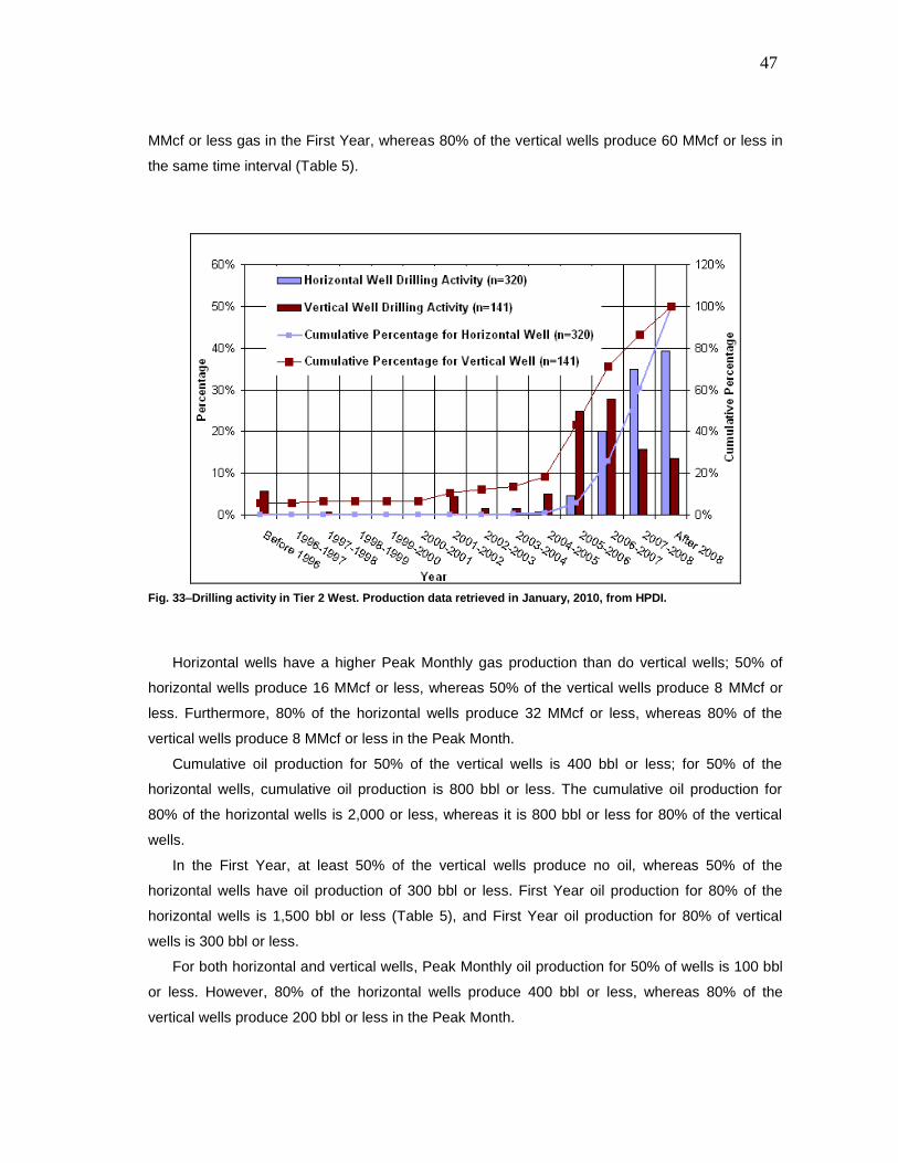
47
MMcf or less gas in the First Year, whereas 80% of the vertical wells produce 60 MMcf or less in
the same time interval (Table 5).
Fig. 33–Drilling activity in Tier 2 West. Production data retrieved in January, 2010, from HPDI.
Horizontal wells have a higher Peak Monthly gas production than do vertical wells; 50% of
horizontal wells produce 16 MMcf or less, whereas 50% of the vertical wells produce 8 MMcf or
less. Furthermore, 80% of the horizontal wells produce 32 MMcf or less, whereas 80% of the
vertical wells produce 8 MMcf or less in the Peak Month.
Cumulative oil production for 50% of the vertical wells is 400 bbl or less; for 50% of the
horizontal wells, cumulative oil production is 800 bbl or less. The cumulative oil production for
80% of the horizontal wells is 2,000 or less, whereas it is 800 bbl or less for 80% of the vertical
wells.
In the First Year, at least 50% of the vertical wells produce no oil, whereas 50% of the
horizontal wells have oil production of 300 bbl or less. First Year oil production for 80% of the
horizontal wells is 1,500 bbl or less (Table 5), and First Year oil production for 80% of vertical
wells is 300 bbl or less.
For both horizontal and vertical wells, Peak Monthly oil production for 50% of wells is 100 bbl
or less. However, 80% of the horizontal wells produce 400 bbl or less, whereas 80% of the
vertical wells produce 200 bbl or less in the Peak Month.
48
Parker County
Drilling Activities
Barnett Shale gas was developed later in Parker County than the Core and Tier 1 areas, but it
was developed before Tier 2 West (Figs. 31 though 34). Vertical wells were first applied to this
area and vertical drilling peaked in 2004 (Fig. 34). By 2006, the number of horizontal wells drilled
annually exceeded the number of vertical wells (Fig. 34).
Parker County Gas and Oil Production
Cumulative gas production of 50% of the horizontal wells is 300 MMcf or less, whereas it is 100
MMcf or less for vertical wells. Cumulative production for 80% of horizontal wells is 500 MMcf or
less, whereas it is 200 MMcf or less for 80% of the vertical wells.
In the First Year, 50% of the horizontal wells produce 200 MMcf or less, and 50% of the
vertical wells produce 50 MMcf or less in Parker County. Moreover, 80% of the horizontal wells
produce 300 MMcf or less gas in the First Year, whereas 80% of the vertical wells only produce
100 MMcf or less in the same time interval (Table 5).
Fig. 34–Drilling activity in Parker County. Production data retrieved in January, 2010, from HPDI.
Horizontal wells in Parker County have a higher Peak Monthly gas production than do vertical
wells; 50% of horizontal wells produce 30 MMcf or less, whereas 50% of the vertical wells
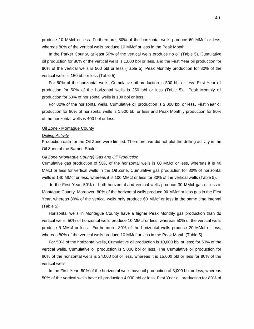
49
produce 10 MMcf or less. Furthermore, 80% of the horizontal wells produce 60 MMcf or less,
whereas 80% of the vertical wells produce 10 MMcf or less in the Peak Month.
In the Parker County, at least 50% of the vertical wells produce no oil (Table 5). Cumulative
oil production for 80% of the vertical wells is 1,000 bbl or less, and the First Year oil production for
80% of the vertical wells is 500 bbl or less (Table 5). Peak Monthly production for 80% of the
vertical wells is 150 bbl or less (Table 5).
For 50% of the horizontal wells, Cumulative oil production is 500 bbl or less. First Year oil
production for 50% of the horizontal wells is 250 bbl or less (Table 5). Peak Monthly oil
production for 50% of horizontal wells is 100 bbl or less.
For 80% of the horizontal wells, Cumulative oil production is 2,000 bbl or less. First Year oil
production for 80% of horizontal wells is 1,500 bbl or less and Peak Monthly production for 80%
of the horizontal wells is 400 bbl or less.
Oil Zone - Montague County
Drilling Activity
Production data for the Oil Zone were limited. Therefore, we did not plot the drilling activity in the
Oil Zone of the Barnett Shale.
Oil Zone (Montague County) Gas and Oil Production
Cumulative gas production of 50% of the horizontal wells is 60 MMcf or less, whereas it is 40
MMcf or less for vertical wells in the Oil Zone. Cumulative gas production for 80% of horizontal
wells is 140 MMcf or less, whereas it is 100 MMcf or less for 80% of the vertical wells (Table 5).
In the First Year, 50% of both horizontal and vertical wells produce 30 MMcf gas or less in
Montague County. Moreover, 80% of the horizontal wells produce 90 MMcf or less gas in the First
Year, whereas 80% of the vertical wells only produce 60 MMcf or less in the same time interval
(Table 5).
Horizontal wells in Montague County have a higher Peak Monthly gas production than do
vertical wells; 50% of horizontal wells produce 10 MMcf or less, whereas 50% of the vertical wells
produce 5 MMcf or less. Furthermore, 80% of the horizontal wells produce 20 MMcf or less,
whereas 80% of the vertical wells produce 10 MMcf or less in the Peak Month (Table 5).
For 50% of the horizontal wells, Cumulative oil production is 10,000 bbl or less; for 50% of the
vertical wells, Cumulative oil production is 5,000 bbl or less. The Cumulative oil production for
80% of the horizontal wells is 24,000 bbl or less, whereas it is 15,000 bbl or less for 80% of the
vertical wells.
In the First Year, 50% of the horizontal wells have oil production of 8,000 bbl or less, whereas
50% of the vertical wells have oil production 4,000 bbl or less. First Year oil production for 80% of
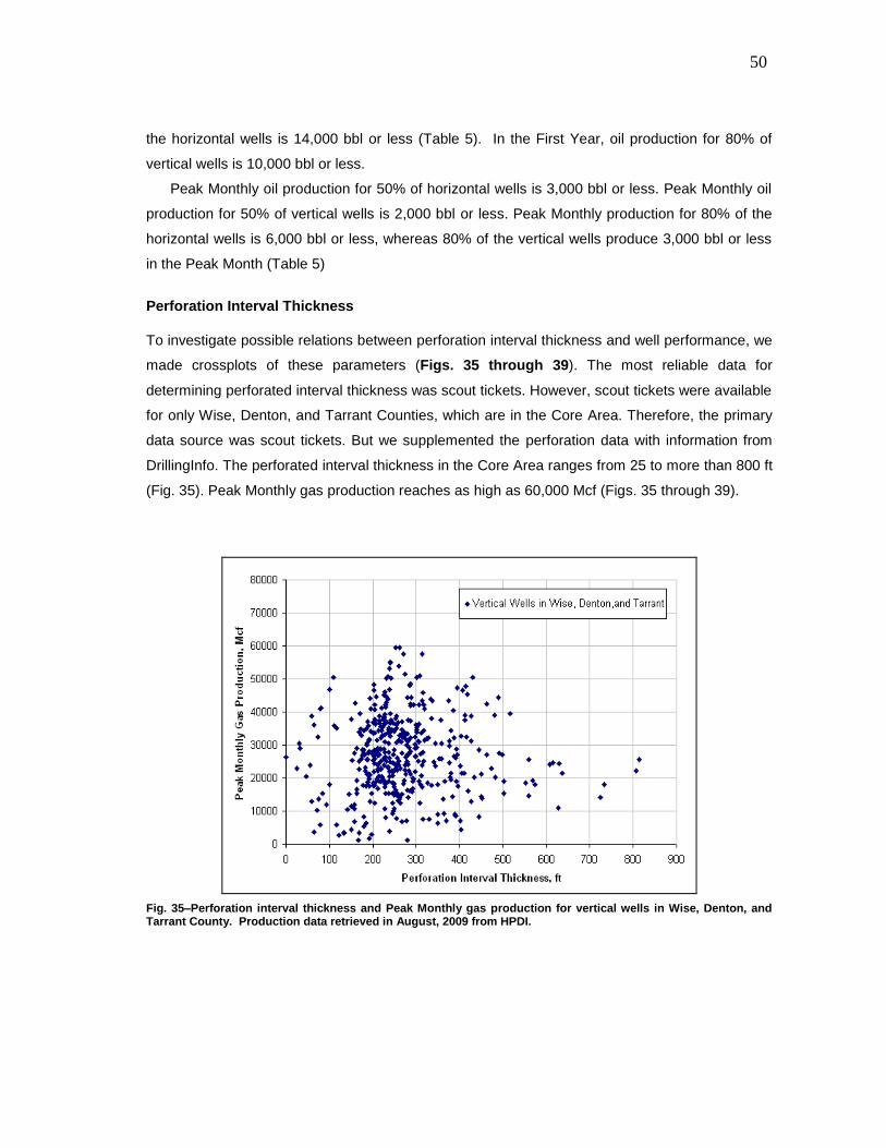
50
the horizontal wells is 14,000 bbl or less (Table 5). In the First Year, oil production for 80% of
vertical wells is 10,000 bbl or less.
Peak Monthly oil production for 50% of horizontal wells is 3,000 bbl or less. Peak Monthly oil
production for 50% of vertical wells is 2,000 bbl or less. Peak Monthly production for 80% of the
horizontal wells is 6,000 bbl or less, whereas 80% of the vertical wells produce 3,000 bbl or less
in the Peak Month (Table 5)
Perforation Interval Thickness
To investigate possible relations between perforation interval thickness and well performance, we
made crossplots of these parameters (Figs. 35 through 39). The most reliable data for
determining perforated interval thickness was scout tickets. However, scout tickets were available
for only Wise, Denton, and Tarrant Counties, which are in the Core Area. Therefore, the primary
data source was scout tickets. But we supplemented the perforation data with information from
DrillingInfo. The perforated interval thickness in the Core Area ranges from 25 to more than 800 ft
(Fig. 35). Peak Monthly gas production reaches as high as 60,000 Mcf (Figs. 35 through 39).
Fig. 35–Perforation interval thickness and Peak Monthly gas production for vertical wells in Wise, Denton, and Tarrant County. Production data retrieved in August, 2009 from HPDI.
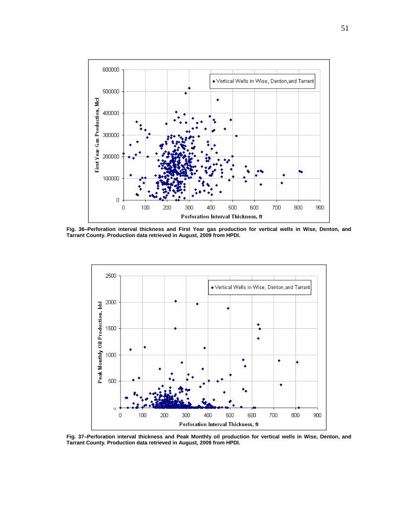
51
Fig. 36–Perforation interval thickness and First Year gas production for vertical wells in Wise, Denton, and Tarrant County. Production data retrieved in August, 2009 from HPDI.
Fig. 37–Perforation interval thickness and Peak Monthly oil production for vertical wells in Wise, Denton, and Tarrant County. Production data retrieved in August, 2009 from HPDI.
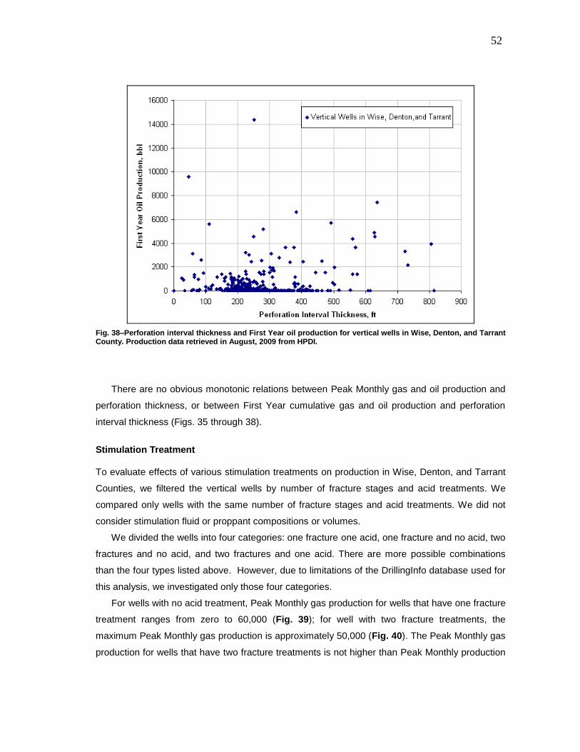
52
Fig. 38–Perforation interval thickness and First Year oil production for vertical wells in Wise, Denton, and Tarrant County. Production data retrieved in August, 2009 from HPDI.
There are no obvious monotonic relations between Peak Monthly gas and oil production and
perforation thickness, or between First Year cumulative gas and oil production and perforation
interval thickness (Figs. 35 through 38).
Stimulation Treatment
To evaluate effects of various stimulation treatments on production in Wise, Denton, and Tarrant
Counties, we filtered the vertical wells by number of fracture stages and acid treatments. We
compared only wells with the same number of fracture stages and acid treatments. We did not
consider stimulation fluid or proppant compositions or volumes.
We divided the wells into four categories: one fracture one acid, one fracture and no acid, two
fractures and no acid, and two fractures and one acid. There are more possible combinations
than the four types listed above. However, due to limitations of the DrillingInfo database used for
this analysis, we investigated only those four categories.
For wells with no acid treatment, Peak Monthly gas production for wells that have one fracture
treatment ranges from zero to 60,000 (Fig. 39); for well with two fracture treatments, the
maximum Peak Monthly gas production is approximately 50,000 (Fig. 40). The Peak Monthly gas
production for wells that have two fracture treatments is not higher than Peak Monthly production
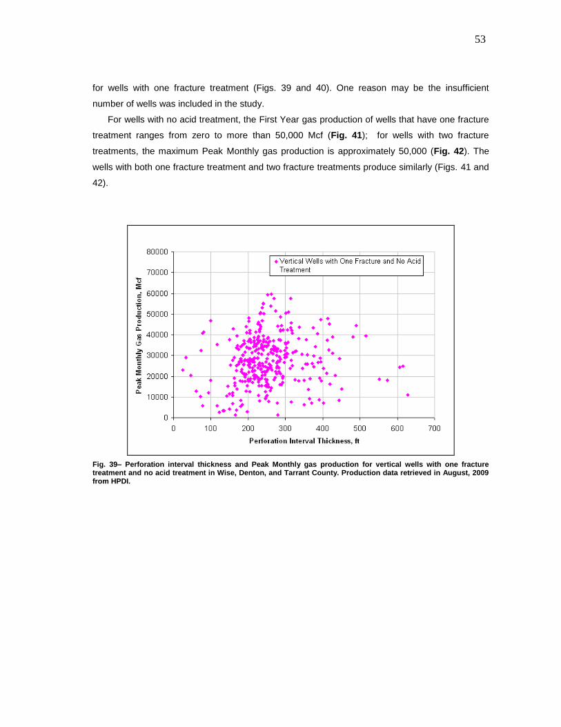
53
for wells with one fracture treatment (Figs. 39 and 40). One reason may be the insufficient
number of wells was included in the study.
For wells with no acid treatment, the First Year gas production of wells that have one fracture
treatment ranges from zero to more than 50,000 Mcf (Fig. 41); for wells with two fracture
treatments, the maximum Peak Monthly gas production is approximately 50,000 (Fig. 42). The
wells with both one fracture treatment and two fracture treatments produce similarly (Figs. 41 and
42).
Fig. 39– Perforation interval thickness and Peak Monthly gas production for vertical wells with one fracture treatment and no acid treatment in Wise, Denton, and Tarrant County. Production data retrieved in August, 2009 from HPDI.
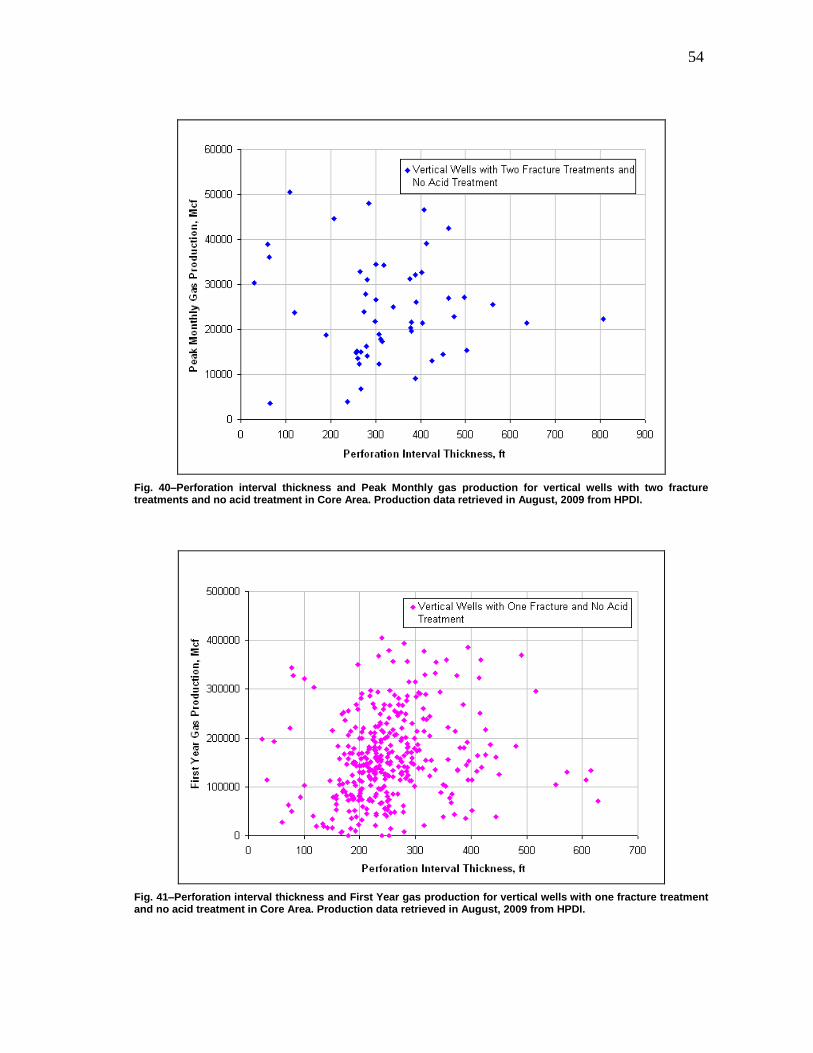
54
Fig. 40–Perforation interval thickness and Peak Monthly gas production for vertical wells with two fracture treatments and no acid treatment in Core Area. Production data retrieved in August, 2009 from HPDI.
Fig. 41–Perforation interval thickness and First Year gas production for vertical wells with one fracture treatment and no acid treatment in Core Area. Production data retrieved in August, 2009 from HPDI.
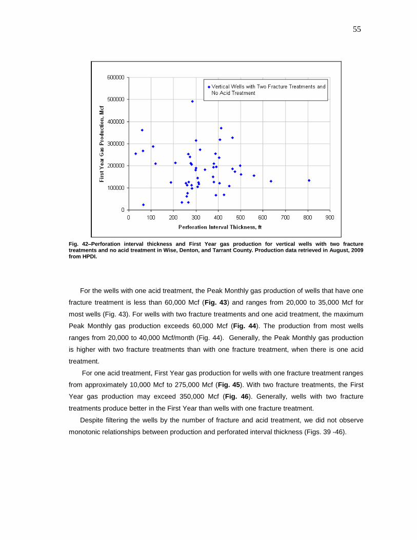
55
Fig. 42–Perforation interval thickness and First Year gas production for vertical wells with two fracture treatments and no acid treatment in Wise, Denton, and Tarrant County. Production data retrieved in August, 2009 from HPDI.
For the wells with one acid treatment, the Peak Monthly gas production of wells that have one
fracture treatment is less than 60,000 Mcf (Fig. 43) and ranges from 20,000 to 35,000 Mcf for
most wells (Fig. 43). For wells with two fracture treatments and one acid treatment, the maximum
Peak Monthly gas production exceeds 60,000 Mcf (Fig. 44). The production from most wells
ranges from 20,000 to 40,000 Mcf/month (Fig. 44). Generally, the Peak Monthly gas production
is higher with two fracture treatments than with one fracture treatment, when there is one acid
treatment.
For one acid treatment, First Year gas production for wells with one fracture treatment ranges
from approximately 10,000 Mcf to 275,000 Mcf (Fig. 45). With two fracture treatments, the First
Year gas production may exceed 350,000 Mcf (Fig. 46). Generally, wells with two fracture
treatments produce better in the First Year than wells with one fracture treatment.
Despite filtering the wells by the number of fracture and acid treatment, we did not observe
monotonic relationships between production and perforated interval thickness (Figs. 39 -46).
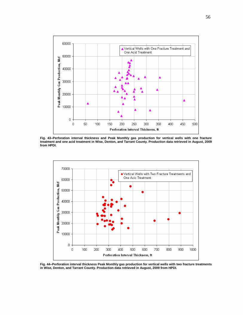
56
Fig. 43–Perforation interval thickness and Peak Monthly gas production for vertical wells with one fracture treatment and one acid treatment in Wise, Denton, and Tarrant County. Production data retrieved in August, 2009 from HPDI.
Fig. 44–Perforation interval thickness Peak Monthly gas production for vertical wells with two fracture treatments in Wise, Denton, and Tarrant County. Production data retrieved in August, 2009 from HPDI.
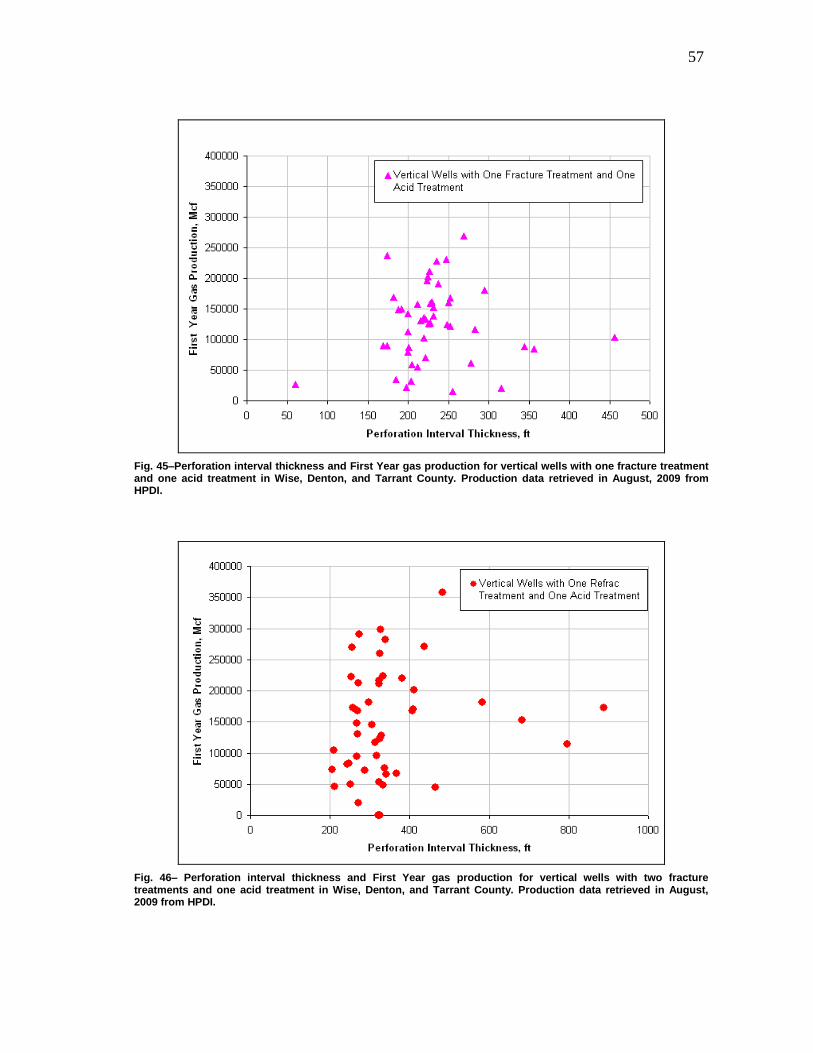
57
Fig. 45–Perforation interval thickness and First Year gas production for vertical wells with one fracture treatment and one acid treatment in Wise, Denton, and Tarrant County. Production data retrieved in August, 2009 from HPDI.
Fig. 46– Perforation interval thickness and First Year gas production for vertical wells with two fracture treatments and one acid treatment in Wise, Denton, and Tarrant County. Production data retrieved in August, 2009 from HPDI.
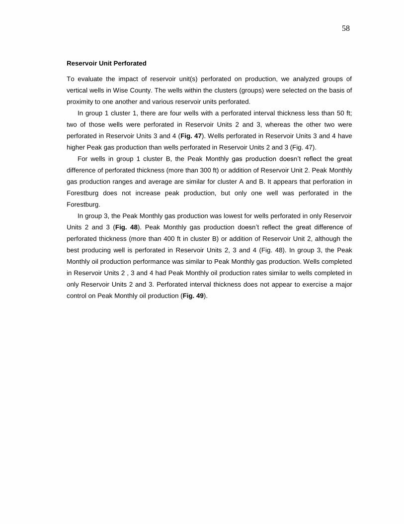
58
Reservoir Unit Perforated
To evaluate the impact of reservoir unit(s) perforated on production, we analyzed groups of
vertical wells in Wise County. The wells within the clusters (groups) were selected on the basis of
proximity to one another and various reservoir units perforated.
In group 1 cluster 1, there are four wells with a perforated interval thickness less than 50 ft;
two of those wells were perforated in Reservoir Units 2 and 3, whereas the other two were
perforated in Reservoir Units 3 and 4 (Fig. 47). Wells perforated in Reservoir Units 3 and 4 have
higher Peak gas production than wells perforated in Reservoir Units 2 and 3 (Fig. 47).
For wells in group 1 cluster B, the Peak Monthly gas production doesn’t reflect the great
difference of perforated thickness (more than 300 ft) or addition of Reservoir Unit 2. Peak Monthly
gas production ranges and average are similar for cluster A and B. It appears that perforation in
Forestburg does not increase peak production, but only one well was perforated in the
Forestburg.
In group 3, the Peak Monthly gas production was lowest for wells perforated in only Reservoir
Units 2 and 3 (Fig. 48). Peak Monthly gas production doesn’t reflect the great difference of
perforated thickness (more than 400 ft in cluster B) or addition of Reservoir Unit 2, although the
best producing well is perforated in Reservoir Units 2, 3 and 4 (Fig. 48). In group 3, the Peak
Monthly oil production performance was similar to Peak Monthly gas production. Wells completed
in Reservoir Units 2 , 3 and 4 had Peak Monthly oil production rates similar to wells completed in
only Reservoir Units 2 and 3. Perforated interval thickness does not appear to exercise a major
control on Peak Monthly oil production (Fig. 49).
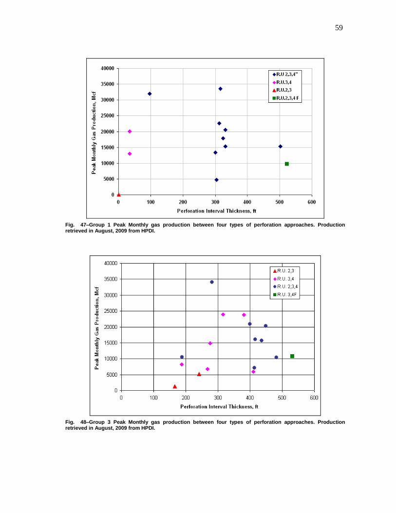
59
Fig. 47–Group 1 Peak Monthly gas production between four types of perforation approaches. Production retrieved in August, 2009 from HPDI.
Fig. 48–Group 3 Peak Monthly gas production between four types of perforation approaches. Production retrieved in August, 2009 from HPDI.
60
Fig. 49–Comparison of Peak Monthly oil production between four types of perforation approaches. Production retrieved in August, 2009 from HPDI.
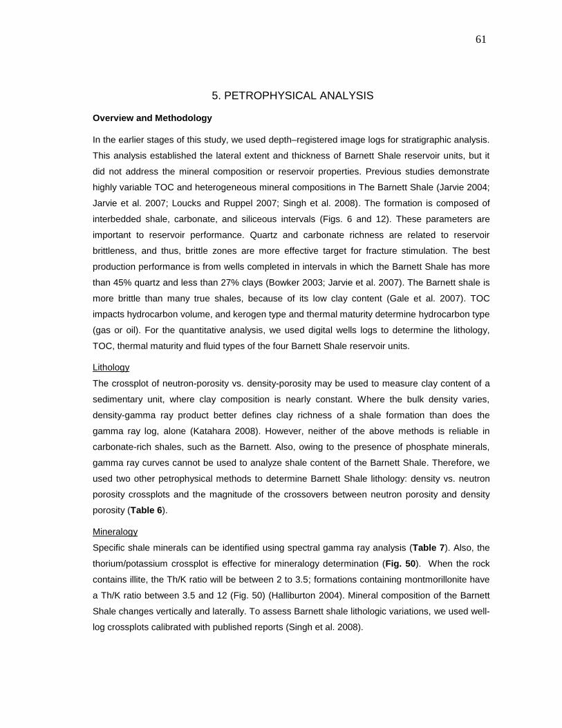
61
5. PETROPHYSICAL ANALYSIS
Overview and Methodology
In the earlier stages of this study, we used depth–registered image logs for stratigraphic analysis.
This analysis established the lateral extent and thickness of Barnett Shale reservoir units, but it
did not address the mineral composition or reservoir properties. Previous studies demonstrate
highly variable TOC and heterogeneous mineral compositions in The Barnett Shale (Jarvie 2004;
Jarvie et al. 2007; Loucks and Ruppel 2007; Singh et al. 2008). The formation is composed of
interbedded shale, carbonate, and siliceous intervals (Figs. 6 and 12). These parameters are
important to reservoir performance. Quartz and carbonate richness are related to reservoir
brittleness, and thus, brittle zones are more effective target for fracture stimulation. The best
production performance is from wells completed in intervals in which the Barnett Shale has more
than 45% quartz and less than 27% clays (Bowker 2003; Jarvie et al. 2007). The Barnett shale is
more brittle than many true shales, because of its low clay content (Gale et al. 2007). TOC
impacts hydrocarbon volume, and kerogen type and thermal maturity determine hydrocarbon type
(gas or oil). For the quantitative analysis, we used digital wells logs to determine the lithology,
TOC, thermal maturity and fluid types of the four Barnett Shale reservoir units.
Lithology
The crossplot of neutron-porosity vs. density-porosity may be used to measure clay content of a
sedimentary unit, where clay composition is nearly constant. Where the bulk density varies,
density-gamma ray product better defines clay richness of a shale formation than does the
gamma ray log, alone (Katahara 2008). However, neither of the above methods is reliable in
carbonate-rich shales, such as the Barnett. Also, owing to the presence of phosphate minerals,
gamma ray curves cannot be used to analyze shale content of the Barnett Shale. Therefore, we
used two other petrophysical methods to determine Barnett Shale lithology: density vs. neutron
porosity crossplots and the magnitude of the crossovers between neutron porosity and density
porosity (Table 6).
Mineralogy
Specific shale minerals can be identified using spectral gamma ray analysis (Table 7). Also, the
thorium/potassium crossplot is effective for mineralogy determination (Fig. 50). When the rock
contains illite, the Th/K ratio will be between 2 to 3.5; formations containing montmorillonite have
a Th/K ratio between 3.5 and 12 (Fig. 50) (Halliburton 2004). Mineral composition of the Barnett
Shale changes vertically and laterally. To assess Barnett shale lithologic variations, we used well-
log crossplots calibrated with published reports (Singh et al. 2008).
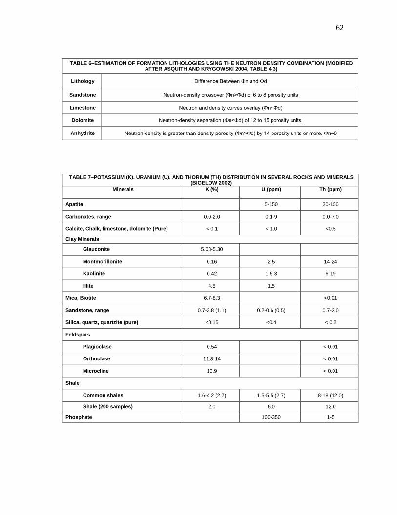
62
TABLE 6–ESTIMATION OF FORMATION LITHOLOGIES USING THE NEUTRON DENSITY COMBINATION (MODIFIED AFTER ASQUITH AND KRYGOWSKI 2004, TABLE 4.3)
Lithology Difference Between Φn and Φd
Sandstone Neutron-density crossover (Φn>Φd) of 6 to 8 porosity units
Limestone Neutron and density curves overlay (Φn~Φd)
Dolomite Neutron-density separation (Φn<Φd) of 12 to 15 porosity units.
Anhydrite Neutron-density is greater than density porosity (Φn>Φd) by 14 porosity units or more. Φn~0
TABLE 7–POTASSIUM (K), URANIUM (U), AND THORIUM (TH) DISTRIBUTION IN SEVERAL ROCKS AND MINERALS (BIGELOW 2002)
Minerals K (%) U (ppm) Th (ppm)
Apatite 5-150 20-150
Carbonates, range 0.0-2.0 0.1-9 0.0-7.0
Calcite, Chalk, limestone, dolomite (Pure) < 0.1 < 1.0 <0.5
Clay Minerals
Glauconite 5.08-5.30
Montmorillonite 0.16 2-5 14-24
Kaolinite 0.42 1.5-3 6-19
Illite 4.5 1.5
Mica, Biotite 6.7-8.3 <0.01
Sandstone, range 0.7-3.8 (1.1) 0.2-0.6 (0.5) 0.7-2.0
Silica, quartz, quartzite (pure) <0.15 <0.4 < 0.2
Feldspars
Plagioclase 0.54 < 0.01
Orthoclase 11.8-14 < 0.01
Microcline 10.9 < 0.01
Shale
Common shales 1.6-4.2 (2.7) 1.5-5.5 (2.7) 8-18 (12.0)
Shale (200 samples) 2.0 6.0 12.0
Phosphate 100-350 1-5
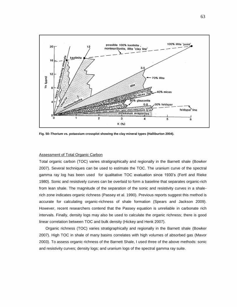
63
Fig. 50–Thorium vs. potassium crossplot showing the clay mineral types (Halliburton 2004).
Assessment of Total Organic Carbon
Total organic carbon (TOC) varies stratigraphically and regionally in the Barnett shale (Bowker
2007). Several techniques can be used to estimate the TOC. The uranium curve of the spectral
gamma ray log has been used for qualitative TOC evaluation since 1930’s (Fertl and Rieke
1980). Sonic and resistively curves can be overlaid to form a baseline that separates organic-rich
from lean shale. The magnitude of the separation of the sonic and resistivity curves in a shale-
rich zone indicates organic richness (Passey et al. 1990). Previous reports suggest this method is
accurate for calculating organic-richness of shale formation (Spears and Jackson 2009).
However, recent researchers contend that the Passey equation is unreliable in carbonate rich
intervals. Finally, density logs may also be used to calculate the organic richness; there is good
linear correlation between TOC and bulk density (Hickey and Henk 2007).
Organic richness (TOC) varies stratigraphically and regionally in the Barnett shale (Bowker
2007). High TOC in shale of many basins correlates with high volumes of absorbed gas (Mavor
2003). To assess organic richness of the Barnett Shale, I used three of the above methods: sonic
and resistivity curves; density logs; and uranium logs of the spectral gamma ray suite.
64
Determination of Shale Thermal Maturity
Previously, Montgomery et al (2005) mapped thermal maturity (vitrinite reflectance) of the Barnett
Shale. To further assess thermal maturity, we applied a maturity index approach proposed by
Zhao et al. (Zhao et al. 2007), using resistivity, neutron and density logs.
Hydrocarbon Type
Identification of hydrocarbon types (oil, condensate, gas) is necessary for optimizing resource
evaluation, completion decisions and production strategies (Tseng et al. 2007). Sonic-neutron
overlays are effective in clarifying hydrocarbon types (Frantz et al. 2005; Johnston 2004), and
thus that is the approach used in this study.
Data Preparation
There were several stages of log processing before we performed petrophysical analysis. Due to
insufficient number of digital triple combo logs that we were provided by IHS, we digitized
selected image logs from MJ system, including neutron porosity, density, density porosity,
acoustic and deep resistivity logs (Fig. 51). Neurolog® was used for digitization. After the
digitizing procedure, we exported the logs in LAS format, which is a format that can be loaded
directly into GeoGraphix® for petrophysical interpretation. In the quantitative analysis, we made a
series of crossplots to evaluate Barnett Shale properties (Figs. 52 through 66).
Normalization is a crucial step for any quantitative petrophysical analysis, especially in
regional multi-well analysis. However, we were unable to normalize the digital well log data
because we were not provided the software requested. As a result, we performed single well
quantitative log analysis.
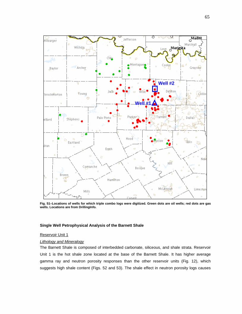
65
Well #2
Well #1
Well #2
Well #1
Fig. 51–Locations of wells for which triple combo logs were digitized. Green dots are oil wells; red dots are gas wells. Locations are from DrillingInfo.
Single Well Petrophysical Analysis of the Barnett Shale
Reservoir Unit 1
Lithology and Mineralogy
The Barnett Shale is composed of interbedded carbonate, siliceous, and shale strata. Reservoir
Unit 1 is the hot shale zone located at the base of the Barnett Shale. It has higher average
gamma ray and neutron porosity responses than the other reservoir units (Fig. 12), which
suggests high shale content (Figs. 52 and 53). The shale effect in neutron porosity logs causes
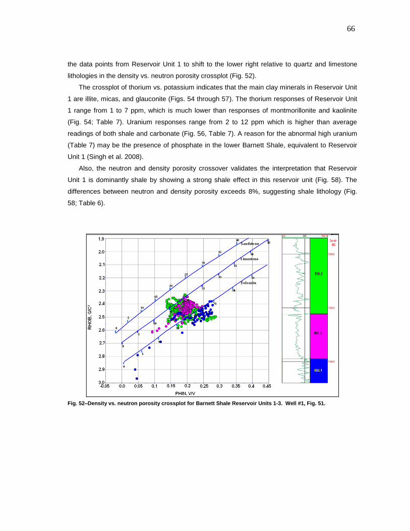
66
the data points from Reservoir Unit 1 to shift to the lower right relative to quartz and limestone
lithologies in the density vs. neutron porosity crossplot (Fig. 52).
The crossplot of thorium vs. potassium indicates that the main clay minerals in Reservoir Unit
1 are illite, micas, and glauconite (Figs. 54 through 57). The thorium responses of Reservoir Unit
1 range from 1 to 7 ppm, which is much lower than responses of montmorillonite and kaolinite
(Fig. 54; Table 7). Uranium responses range from 2 to 12 ppm which is higher than average
readings of both shale and carbonate (Fig. 56, Table 7). A reason for the abnormal high uranium
(Table 7) may be the presence of phosphate in the lower Barnett Shale, equivalent to Reservoir
Unit 1 (Singh et al. 2008).
Also, the neutron and density porosity crossover validates the interpretation that Reservoir
Unit 1 is dominantly shale by showing a strong shale effect in this reservoir unit (Fig. 58). The
differences between neutron and density porosity exceeds 8%, suggesting shale lithology (Fig.
58; Table 6).
Fig. 52–Density vs. neutron porosity crossplot for Barnett Shale Reservoir Units 1-3. Well #1, Fig. 51.
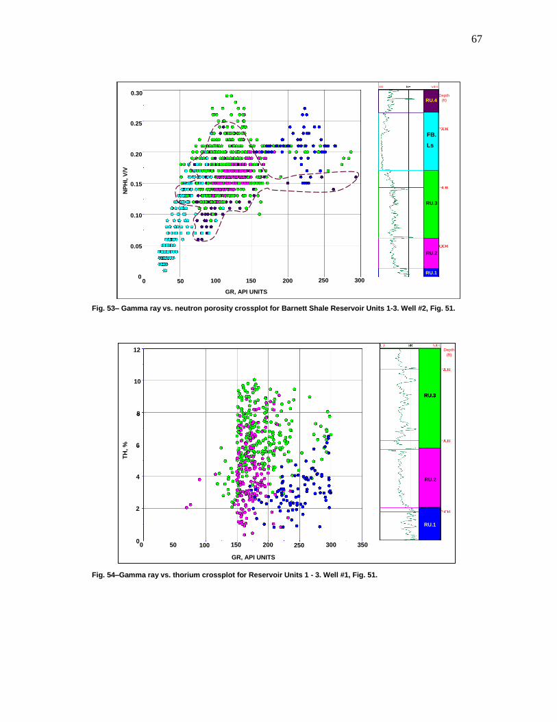
67
0.30
0.25
0.15
0.20
0.10
0.05
0100 300150 200 25050
GR, API UNITS
0
NP
HI,
V/V
RU.1
RU.2
RU.3
RU.4
FB.
Ls
Depth
(ft)
0.30
0.25
0.15
0.20
0.10
0.05
0100 300150 200 25050
GR, API UNITS
0
NP
HI,
V/V
0.30
0.25
0.15
0.20
0.10
0.05
0100 300150 200 25050
GR, API UNITS
0
NP
HI,
V/V
RU.1
RU.2
RU.3
RU.4
FB.
Ls
Depth
(ft)
Fig. 53– Gamma ray vs. neutron porosity crossplot for Barnett Shale Reservoir Units 1-3. Well #2, Fig. 51.
TH
, %
150 250 300 3501000
6
8
4
12
2
10
GR, API UNITS
500 200
RU.1
RU.2
RU.3
Depth
(ft)
TH
, %
150 250 300 3501000
6
8
4
12
2
10
GR, API UNITS
500 200
RU.1
RU.2
RU.3
TH
, %
150 250 300 3501000
6
8
4
12
2
10
GR, API UNITS
500 200
TH
, %
150 250 300 3501000
6
8
4
12
2
10
GR, API UNITS
500 200
TH
, %
150 250 300 3501000
6
8
4
12
2
10
GR, API UNITS
500 200150 250 300 3501000
6
8
4
12
2
10
0
6
8
4
12
2
10
GR, API UNITS
500 200
RU.1
RU.2
RU.3
RU.1
RU.2
RU.3
Depth
(ft)
Fig. 54–Gamma ray vs. thorium crossplot for Reservoir Units 1 - 3. Well #1, Fig. 51.
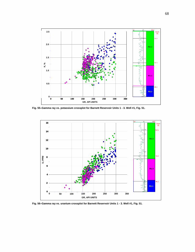
68
1.5
2.0
1.0
0.5
0
2.5
0 50 150 200 250 300 350100
GR, API UNITS
K,
%
RU.1
RU.2
RU.3
Depth
(ft)
1.5
2.0
1.0
0.5
0
2.5
0 50 150 200 250 300 350100
GR, API UNITS
K,
%
RU.1
RU.2
RU.3
1.5
2.0
1.0
0.5
0
2.5
0 50 150 200 250 300 350100
GR, API UNITS
K,
%
1.5
2.0
1.0
0.5
0
2.5
0 50 150 200 250 300 3501000 50 150 200 250 300 350100
GR, API UNITS
K,
%
RU.1
RU.2
RU.3
Depth
(ft)
Fig. 55–Gamma ray vs. potassium crossplot for Barnett Reservoir Units 1 - 3. Well #1, Fig. 51.
U, P
PM
2
0
4
14
6
10
16
8
12
GR, API UNITS
50 150 200 250 300 3501000
RU.1
RU.2
RU.3
Depth
(ft)
U, P
PM
2
0
4
14
6
10
16
8
12
GR, API UNITS
50 150 200 250 300 3501000
U, P
PM
2
0
4
14
6
10
16
8
12
2
0
4
14
6
10
16
8
12
GR, API UNITS
50 150 200 250 300 3501000
RU.1
RU.2
RU.3
RU.1
RU.2
RU.3
Depth
(ft)
Fig. 56–Gamma ray vs. uranium crossplot for Barnett Reservoir Units 1 - 3. Well #1, Fig. 51.
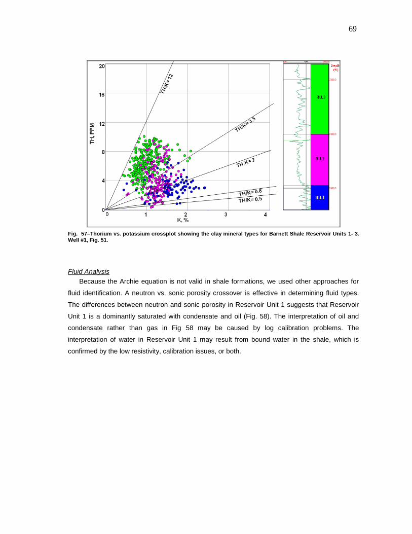
69
Fig. 57–Thorium vs. potassium crossplot showing the clay mineral types for Barnett Shale Reservoir Units 1- 3. Well #1, Fig. 51.
Fluid Analysis
Because the Archie equation is not valid in shale formations, we used other approaches for
fluid identification. A neutron vs. sonic porosity crossover is effective in determining fluid types.
The differences between neutron and sonic porosity in Reservoir Unit 1 suggests that Reservoir
Unit 1 is a dominantly saturated with condensate and oil (Fig. 58). The interpretation of oil and
condensate rather than gas in Fig 58 may be caused by log calibration problems. The
interpretation of water in Reservoir Unit 1 may result from bound water in the shale, which is
confirmed by the low resistivity, calibration issues, or both.
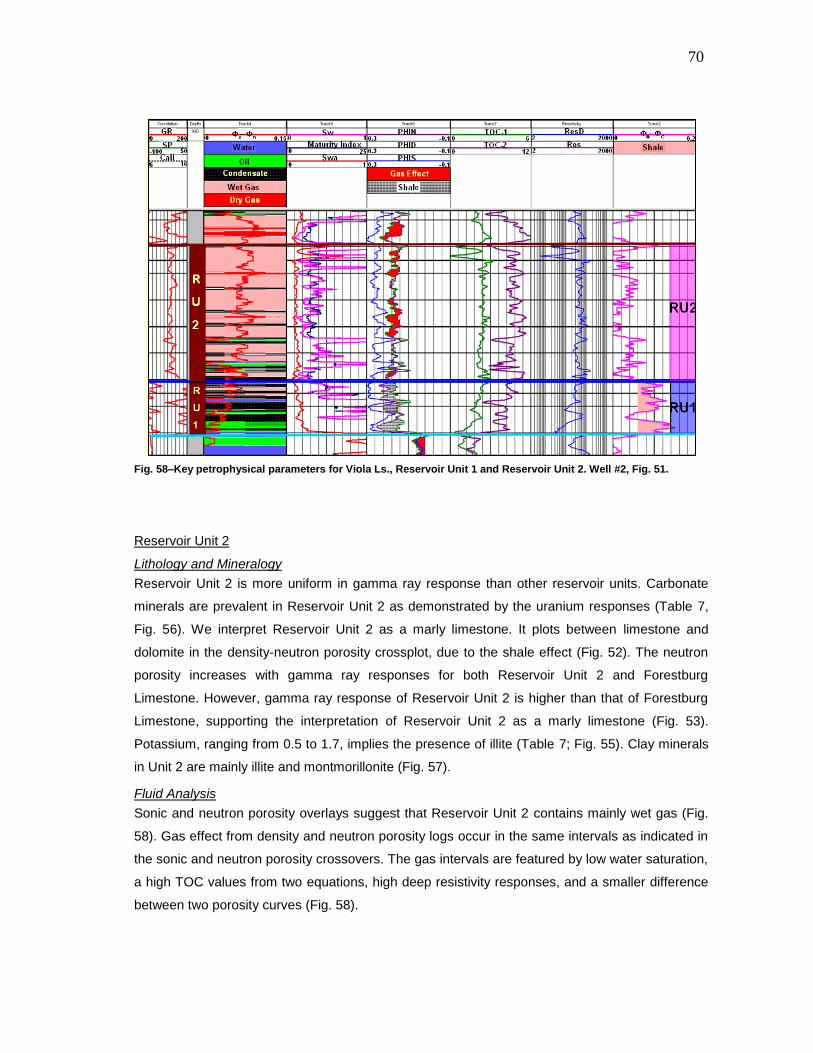
70
Fig. 58–Key petrophysical parameters for Viola Ls., Reservoir Unit 1 and Reservoir Unit 2. Well #2, Fig. 51.
Reservoir Unit 2
Lithology and Mineralogy
Reservoir Unit 2 is more uniform in gamma ray response than other reservoir units. Carbonate
minerals are prevalent in Reservoir Unit 2 as demonstrated by the uranium responses (Table 7,
Fig. 56). We interpret Reservoir Unit 2 as a marly limestone. It plots between limestone and
dolomite in the density-neutron porosity crossplot, due to the shale effect (Fig. 52). The neutron
porosity increases with gamma ray responses for both Reservoir Unit 2 and Forestburg
Limestone. However, gamma ray response of Reservoir Unit 2 is higher than that of Forestburg
Limestone, supporting the interpretation of Reservoir Unit 2 as a marly limestone (Fig. 53).
Potassium, ranging from 0.5 to 1.7, implies the presence of illite (Table 7; Fig. 55). Clay minerals
in Unit 2 are mainly illite and montmorillonite (Fig. 57).
Fluid Analysis
Sonic and neutron porosity overlays suggest that Reservoir Unit 2 contains mainly wet gas (Fig.
58). Gas effect from density and neutron porosity logs occur in the same intervals as indicated in
the sonic and neutron porosity crossovers. The gas intervals are featured by low water saturation,
a high TOC values from two equations, high deep resistivity responses, and a smaller difference
between two porosity curves (Fig. 58).

71
Reservoir Unit 3
Lithology
Reservoir Unit 3 is composed of stacked, upward coarsening sequences that result in highly
heterogeneous reservoir properties and log responses (Fig. 12). Reservoir Unit 3 has a wide
range of density and neutron porosity indicating presence of silica-rich intervals, limestone and
dolomite (Figs. 52 and 59). The strong silica responses are higher than those of Reservoir Units 1
and 2 (Fig. 52). This siliceous quality may make Reservoir Unit 3 a better target for fracture
stimulation (Figs. 52 and 59).
The neutron porosity of Reservoir Unit 3 falls into two zones in the cross plot (Fig. 60). The
intervals with gamma ray response from 100 API to 150 API show a range of neutron porosity
responses (Fig. 60). The interval with high gamma ray response has an average neutron porosity
of 0.2 (Fig. 60).
Fig. 59 – Neutron porosity vs. density cross-plot for Reservoir Units 3 and 4 and Forestburg Limestone. Well #1, Fig. 51.
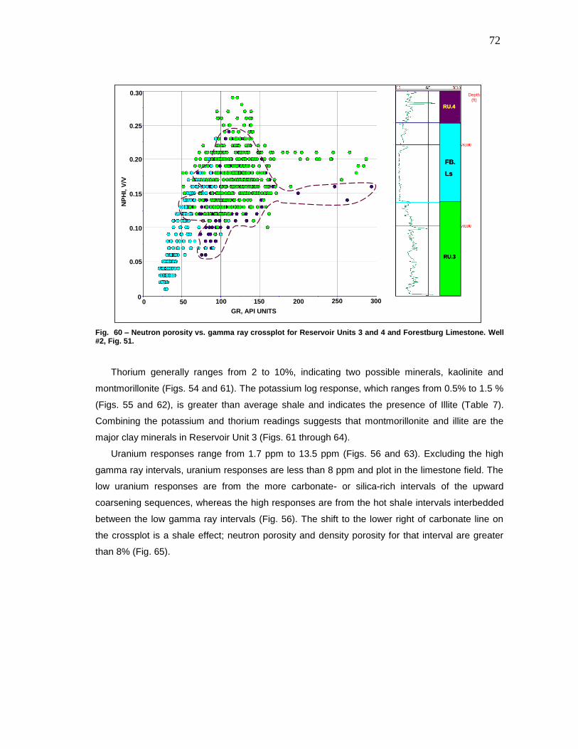
72
0.30
0.25
0.15
0.20
0.10
0.05
0100 300150 200 25050
GR, API UNITS
0
NP
HI,
V/V
RU.3
RU.4
FB.
Ls
Depth
(ft)
0.30
0.25
0.15
0.20
0.10
0.05
0100 300150 200 25050
GR, API UNITS
0
NP
HI,
V/V
RU.3
RU.4
FB.
Ls
RU.3
RU.4
FB.
Ls
Depth
(ft)
Fig. 60 – Neutron porosity vs. gamma ray crossplot for Reservoir Units 3 and 4 and Forestburg Limestone. Well #2, Fig. 51.
Thorium generally ranges from 2 to 10%, indicating two possible minerals, kaolinite and
montmorillonite (Figs. 54 and 61). The potassium log response, which ranges from 0.5% to 1.5 %
(Figs. 55 and 62), is greater than average shale and indicates the presence of Illite (Table 7).
Combining the potassium and thorium readings suggests that montmorillonite and illite are the
major clay minerals in Reservoir Unit 3 (Figs. 61 through 64).
Uranium responses range from 1.7 ppm to 13.5 ppm (Figs. 56 and 63). Excluding the high
gamma ray intervals, uranium responses are less than 8 ppm and plot in the limestone field. The
low uranium responses are from the more carbonate- or silica-rich intervals of the upward
coarsening sequences, whereas the high responses are from the hot shale intervals interbedded
between the low gamma ray intervals (Fig. 56). The shift to the lower right of carbonate line on
the crossplot is a shale effect; neutron porosity and density porosity for that interval are greater
than 8% (Fig. 65).
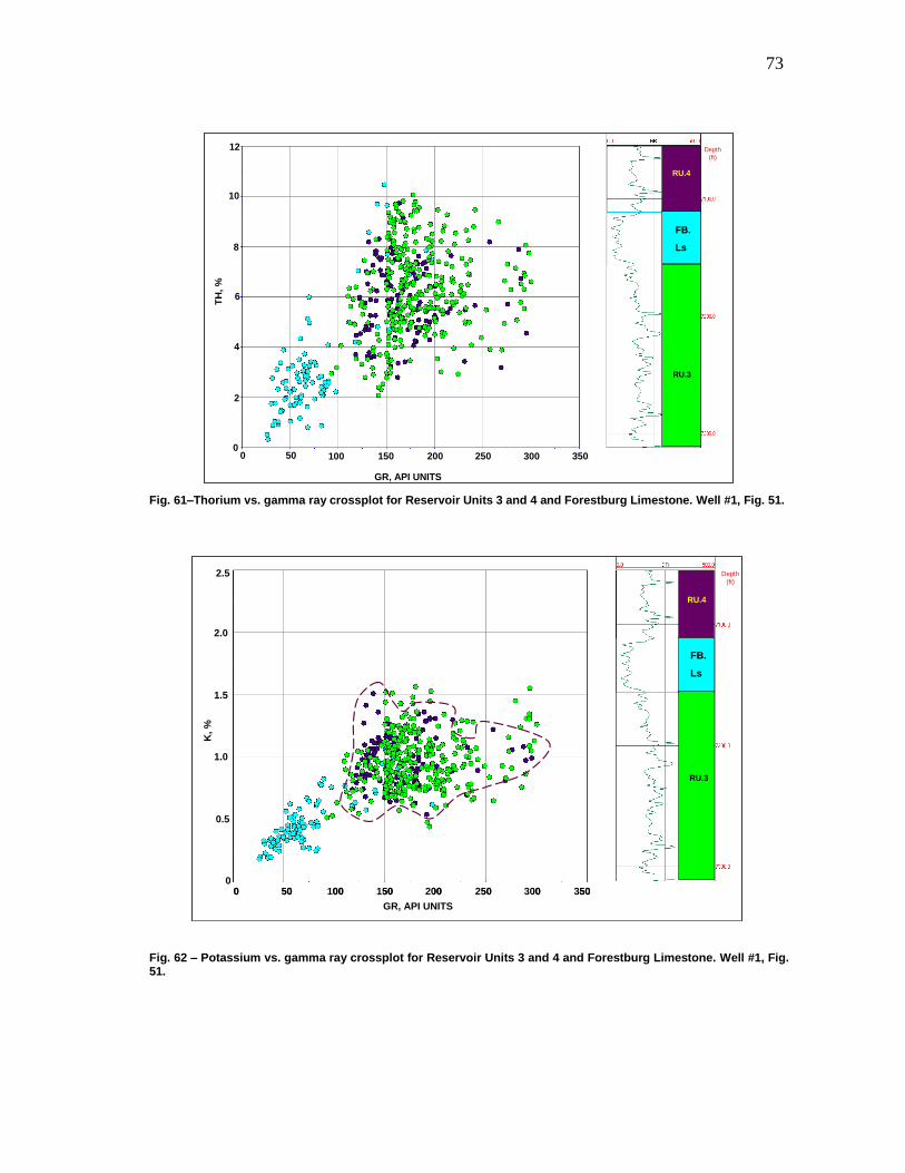
73
TH
, %
150 250 300 3501000
6
8
4
12
2
10
GR, API UNITS
50 2000
RU.3
RU.4
FB.
Ls
Depth
(ft)
TH
, %
150 250 300 3501000
6
8
4
12
2
10
GR, API UNITS
50 2000
RU.3
RU.4
FB.
Ls
Depth
(ft)
Fig. 61–Thorium vs. gamma ray crossplot for Reservoir Units 3 and 4 and Forestburg Limestone. Well #1, Fig. 51.
1.5
2.0
1.0
0.5
0
2.5
0 50 150 200 250 300 350100
GR, API UNITS
K,
%
RU.3
RU.4
FB.
Ls
Depth
(ft)
1.5
2.0
1.0
0.5
0
2.5
0 50 150 200 250 300 350100
GR, API UNITS
K,
%
1.5
2.0
1.0
0.5
0
2.5
0 50 150 200 250 300 3501000 50 150 200 250 300 350100
GR, API UNITS
K,
%
RU.3
RU.4
FB.
Ls
Depth
(ft)
Fig. 62 – Potassium vs. gamma ray crossplot for Reservoir Units 3 and 4 and Forestburg Limestone. Well #1, Fig. 51.
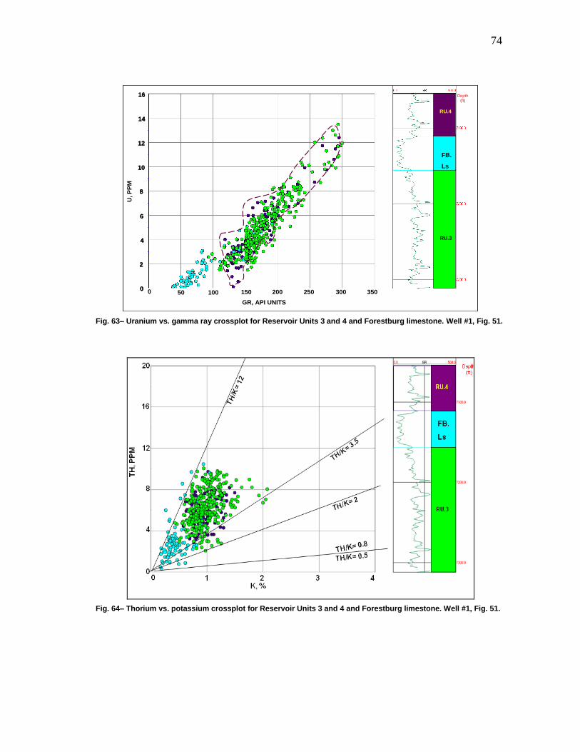
74
U,
PP
M
GR, API UNITS
50 150 200 250 300 3501000
RU.3
RU.4
FB.
Ls
Depth
(ft)
2
0
4
14
6
10
16
8
12
U,
PP
M
GR, API UNITS
50 150 200 250 300 3501000
RU.3
RU.4
FB.
Ls
Depth
(ft)
2
0
4
14
6
10
16
8
12
2
0
4
14
6
10
16
8
12
Fig. 63– Uranium vs. gamma ray crossplot for Reservoir Units 3 and 4 and Forestburg limestone. Well #1, Fig. 51.
Fig. 64– Thorium vs. potassium crossplot for Reservoir Units 3 and 4 and Forestburg limestone. Well #1, Fig. 51.
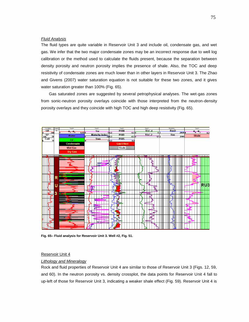
75
Fluid Analysis
The fluid types are quite variable in Reservoir Unit 3 and include oil, condensate gas, and wet
gas. We infer that the two major condensate zones may be an incorrect response due to well log
calibration or the method used to calculate the fluids present, because the separation between
density porosity and neutron porosity implies the presence of shale. Also, the TOC and deep
resistivity of condensate zones are much lower than in other layers in Reservoir Unit 3. The Zhao
and Givens (2007) water saturation equation is not suitable for these two zones, and it gives
water saturation greater than 100% (Fig. 65).
Gas saturated zones are suggested by several petrophysical analyses. The wet-gas zones
from sonic-neutron porosity overlays coincide with those interpreted from the neutron-density
porosity overlays and they coincide with high TOC and high deep resistivity (Fig. 65).
Fig. 65– Fluid analysis for Reservoir Unit 3. Well #2, Fig. 51.
Reservoir Unit 4
Lithology and Mineralogy
Rock and fluid properties of Reservoir Unit 4 are similar to those of Reservoir Unit 3 (Figs. 12, 59,
and 60). In the neutron porosity vs. density crossplot, the data points for Reservoir Unit 4 fall to
up-left of those for Reservoir Unit 3, indicating a weaker shale effect (Fig. 59). Reservoir Unit 4 is
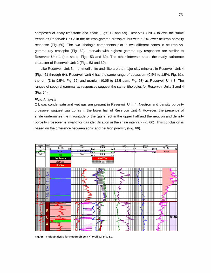
76
composed of shaly limestone and shale (Figs. 12 and 59). Reservoir Unit 4 follows the same
trends as Reservoir Unit 3 in the neutron-gamma crossplot, but with a 5% lower neutron porosity
response (Fig. 60). The two lithologic components plot in two different zones in neutron vs.
gamma ray crossplot (Fig. 60). Intervals with highest gamma ray responses are similar to
Reservoir Unit 1 (hot shale, Figs. 53 and 60). The other intervals share the marly carbonate
character of Reservoir Unit 2 (Figs. 53 and 60).
Like Reservoir Unit 3, montmorillonite and illite are the major clay minerals in Reservoir Unit 4
(Figs. 61 through 64). Reservoir Unit 4 has the same range of potassium (0.5% to 1.5%, Fig. 61),
thorium (3 to 9.5%, Fig. 62) and uranium (0.05 to 12.5 ppm, Fig. 63) as Reservoir Unit 3. The
ranges of spectral gamma ray responses suggest the same lithologies for Reservoir Units 3 and 4
(Fig. 64).
Fluid Analysis
Oil, gas condensate and wet gas are present in Reservoir Unit 4. Neutron and density porosity
crossover suggest gas zones in the lower half of Reservoir Unit 4. However, the presence of
shale undermines the magnitude of the gas effect in the upper half and the neutron and density
porosity crossover is invalid for gas identification in the shale interval (Fig. 66). This conclusion is
based on the difference between sonic and neutron porosity (Fig. 66).
Fig. 66– Fluid analysis for Reservoir Unit 4. Well #2, Fig. 51.
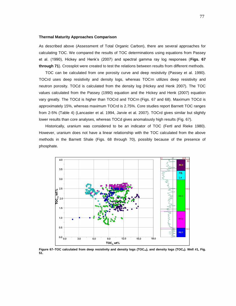
77
Thermal Maturity Approaches Comparison
As described above (Assessment of Total Organic Carbon), there are several approaches for
calculating TOC. We compared the results of TOC determinations using equations from Passey
et al. (1990), Hickey and Henk’s (2007) and spectral gamma ray log responses (Figs. 67
through 71). Crossplot were created to test the relations between results from different methods.
TOC can be calculated from one porosity curve and deep resistivity (Passey et al. 1990).
TOCrd uses deep resistivity and density logs, whereas TOCrn utilizes deep resistivity and
neutron porosity. TOCd is calculated from the density log (Hickey and Henk 2007). The TOC
values calculated from the Passey (1990) equation and the Hickey and Henk (2007) equation
vary greatly. The TOCd is higher than TOCrd and TOCrn (Figs. 67 and 68). Maximum TOCd is
approximately 15%, whereas maximum TOCrd is 2.75%. Core studies report Barnett TOC ranges
from 2-5% (Table 4) (Lancaster et al. 1994, Jarvie et al. 2007). TOCrd gives similar but slightly
lower results than core analyses, whereas TOCd gives anomalously high results (Fig. 67).
Historically, uranium was considered to be an indicator of TOC (Fertl and Rieke 1980).
However, uranium does not have a linear relationship with the TOC calculated from the above
methods in the Barnett Shale (Figs. 68 through 70), possibly because of the presence of
phosphate.
Figure 67–TOC calculated from deep resistivity and density logs (TOCrd), and density logs (TOCd). Well #1, Fig. 51.
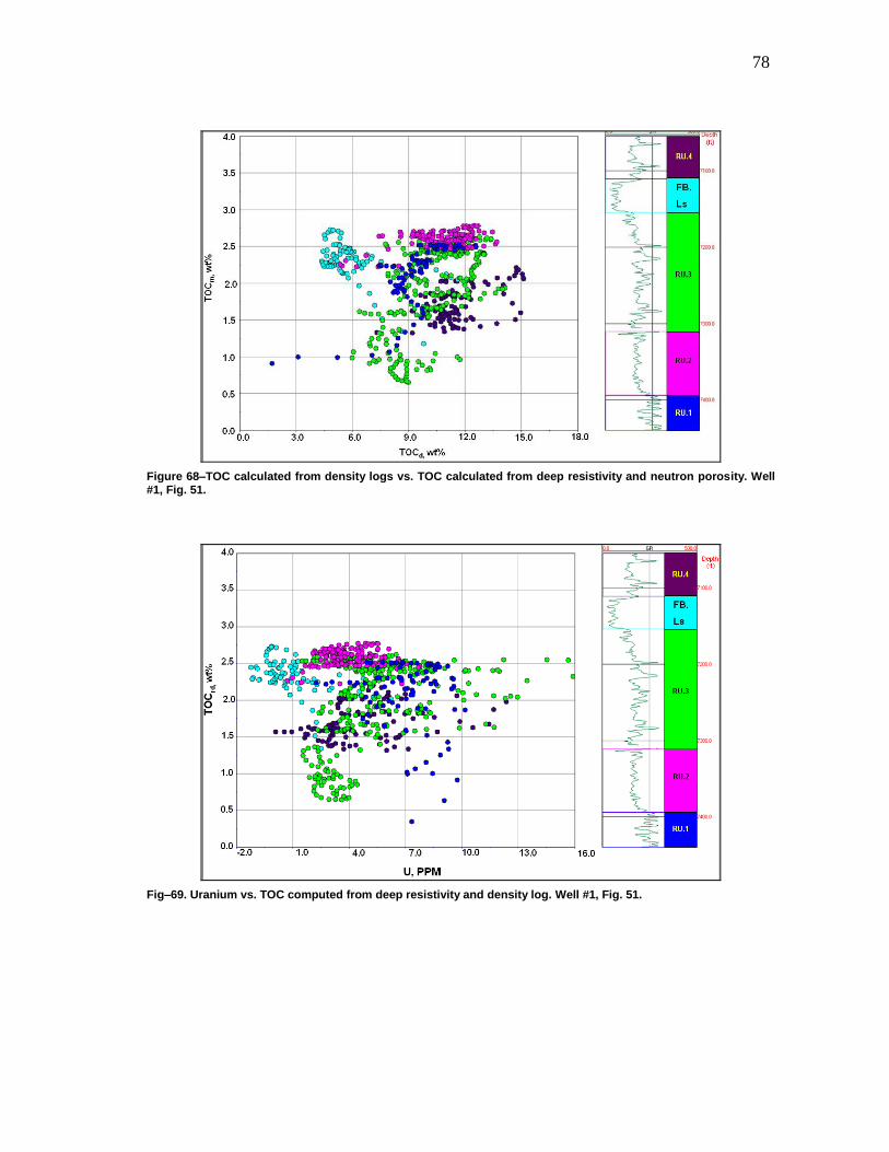
78
Figure 68–TOC calculated from density logs vs. TOC calculated from deep resistivity and neutron porosity. Well #1, Fig. 51.
Fig–69. Uranium vs. TOC computed from deep resistivity and density log. Well #1, Fig. 51.
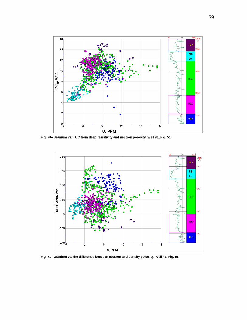
79
Fig. 70– Uranium vs. TOC from deep resistivity and neutron porosity. Well #1, Fig. 51.
Fig. 71– Uranium vs. the difference between neutron and density porosity. Well #1, Fig. 51.
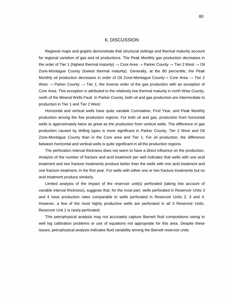
80
6. DISCUSSION
Regional maps and graphs demonstrate that structural settings and thermal maturity account
for regional variation of gas and oil productions. The Peak Monthly gas production decreases in
the order of Tier 1 (highest thermal maturity) → Core Area → Parker County → Tier 2 West → Oil
Zone-Montague County (lowest thermal maturity). Generally, at the 80 percentile, the Peak
Monthly oil production decreases in order of Oil Zone-Montague County→ Core Area → Tier 2
West → Parker County → Tier 1, the inverse order of the gas production with an exception of
Core Area. This exception is attributed to the relatively low thermal maturity in north Wise County,
north of the Mineral Wells Fault. In Parker County, both oil and gas production are intermediate to
production in Tier 1 and Tier 2 West.
Horizontal and vertical wells have quite variable Cumulative, First Year, and Peak Monthly
production among the five production regions. For both oil and gas, production from horizontal
wells is approximately twice as great as the production from vertical wells. The difference in gas
production caused by drilling types is more significant in Parker County, Tier 2 West and Oil
Zone-Montague County than in the Core area and Tier 1. For oil production, the difference
between horizontal and vertical wells is quite significant in all the production regions.
The perforation interval thickness does not seem to have a direct influence on the production.
Analysis of the number of fracture and acid treatment per well indicates that wells with one acid
treatment and two fracture treatments produce better than the wells with one acid treatment and
one fracture treatment, in the first year. For wells with either one or two fracture treatments but no
acid treatment produce similarly.
Limited analysis of the impact of the reservoir unit(s) perforated (taking into account of
variable interval thickness), suggests that, for the most part, wells perforated in Reservoir Units 3
and 4 have production rates comparable to wells perforated in Reservoir Units 2, 3 and 4.
However, a few of the most highly productive wells are perforated in all 3 Reservoir Units.
Reservoir Unit 1 is rarely perforated.
This petrophysical analysis may not accurately capture Barnett fluid compositions owing to
well log calibration problems or use of equations not appropriate for this area. Despite these
issues, petrophysical analysis indicates fluid variability among the Barnett reservoir units.
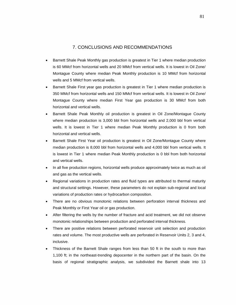
81
7. CONCLUSIONS AND RECOMMENDATIONS
Barnett Shale Peak Monthly gas production is greatest in Tier 1 where median production
is 60 MMcf from horizontal wells and 20 MMcf from vertical wells. It is lowest in Oil Zone/
Montague County where median Peak Monthly production is 10 MMcf from horizontal
wells and 5 MMcf from vertical wells.
Barnett Shale First year gas production is greatest in Tier 1 where median production is
350 MMcf from horizontal wells and 150 MMcf from vertical wells. It is lowest in Oil Zone/
Montague County where median First Year gas production is 30 MMcf from both
horizontal and vertical wells.
Barnett Shale Peak Monthly oil production is greatest in Oil Zone/Montague County
where median production is 3,000 bbl from horizontal wells and 2,000 bbl from vertical
wells. It is lowest in Tier 1 where median Peak Monthly production is 0 from both
horizontal and vertical wells.
Barnett Shale First Year oil production is greatest in Oil Zone/Montague County where
median production is 8,000 bbl from horizontal wells and 4,000 bbl from vertical wells. It
is lowest in Tier 1 where median Peak Monthly production is 0 bbl from both horizontal
and vertical wells.
In all five production regions, horizontal wells produce approximately twice as much as oil
and gas as the vertical wells.
Regional variations in production rates and fluid types are attributed to thermal maturity
and structural settings. However, these parameters do not explain sub-regional and local
variations of production rates or hydrocarbon composition.
There are no obvious monotonic relations between perforation interval thickness and
Peak Monthly or First Year oil or gas production.
After filtering the wells by the number of fracture and acid treatment, we did not observe
monotonic relationships between production and perforated interval thickness.
There are positive relations between perforated reservoir unit selection and production
rates and volume. The most productive wells are perforated in Reservoir Units 2, 3 and 4,
inclusive.
Thickness of the Barnett Shale ranges from less than 50 ft in the south to more than
1,100 ft; in the northeast-trending depocenter in the northern part of the basin. On the
basis of regional stratigraphic analysis, we subdivided the Barnett shale into 13
82
sequences which were upscaled into 4 reservoir units that are consequential to reservoir
engineering decisions.
Reservoir Unit 1, the basal hot shale, is rarely perforated; presence of phosphate
complicates interpretation of shale and TOC content of Reservoir Unit 1. Reservoir Unit 2
is a laminated, siliceous mudstone and marly carbonate zone; it is relatively uniform in
lithology and commonly is perforated. Reservoir Unit 3 is composed of multiple, stacked,
thin, upward coarsening sequences of interbedded shale, carbonate, and siliceous
(brittle) strata; this appears to be the most commonly perforated Barnett reservoir unit.
Reservoir Unit 4, the upper Barnett Shale (where Forestburg Ls. is present), is similar to
Reservoir Unit 3 in lithology and reservoir properties, and it is commonly perforated.
Reservoir Units 1 and 2 have a wide range of clay mineral types, whereas Reservoir
Units 3 and 4 are dominantly montmorillonite.
Petrophysical analysis of three wells, in southern Wise County suggests that: (1) the
dominant fluid in Reservoir Unit 1 is bound water; (2) Reservoir Unit 2 contains
condensate, oil and water; and (3) the fluids in both Reservoir Units 3 and 4 are similar
but highly variable and include water, oil and gas. This petrophysical analysis may not
accurately describe Barnett fluid compositions, owing to well log calibration problems or
use of equations not appropriate for the Core Area. Despite these issues, petrophysical
analysis indicates fluid variability among the Barnett reservoir units.
Petrophysical methods of TOC determination give questionable results compared to the
core analysis.
The following are recommendations resulting from the study:
calibrate well log responses with core descriptions;
further petrophysical studies of reservoir fluids should be conducted with calibrated well
logs;
map regional reservoir properties using normalized digital well log data;
analyze production data, normalized by proppant and fluid volumes and types, well types,
and number of fracture stages; and
develop more accurate equations for Barnett Shale TOC calculation from well logs
calibrated with core samples.
83
REFERENCES
Asquith, G and Krygowski, D. 2004. Basic Well Log Analysis. Tulsa, OK. American Association of
Petroleum Geologists (AAPG). Bigelow, E.L. 2002. Introduction to Wireline Log Analysis-Baker Hughes Atlas. Houston, TX.
Baker Hughes, Inc. Bowker, K.A. 2003. Recent Development of the Barnett Shale Play, Fort Worth Basin. West
Texas Geological Society Bulletin 42(6): 4-11. Bowker, K.A. 2007. Barnett Shale Gas Production, Fort Worth Basin: Issues and Discussion.
AAPG Bulletin 91 (4): 523-533. Daniels, J., Waters, G., LeCalvez, J., Lassek, J., Bentley, D. 2007. Contacting More of the
Barnett Shale through an Integration of Real-Time Microseismic Monitoring, Petrophysics and Hrdraulic Fracture Design. Paper SPE 110562 presented at the 2007 SPE Annual Technical Conference and Exhibition, Anaheim CA, 12-14 October 2007. DOI: 10.2118/110562-MS.
Devon Energy. 2008. Barnett Shale Resource Update. Oklahoma City, OK.
http://www.devonenergy.com/ir/Documents/032808%20-%20Barnett%20and%20Resource%20Update.pdf. Accessed March 28 2008.
Energy Information Administration (EIA). 2006. The Northeast Natural Gas Market in 2030.
Washington, DC http://www.eia.doe.gov/pub/oil_gas/natural_gas/presentations/2006/ngmarket/ngmarket_files/frame.html. Accessed April 2008.
Energy Information Administration (EIA). 2007. Natrual Gas Imports by County. Washington, DC.
http://tonto.eia.doe.gov/dnav/ng/ng_move_impc_s1_a.htm. Accessed April 2008. Energy Information Administration (EIA). 2008. Natrual Gas Production. Washington, DC.
http://tonto.eia.doe.gov/dnav/ng/ng_prod_sum_dcu_NUS_a.htm. Accessed April 2008. Energy Information Administration (EIA). 2009. Shale Gas Plays, Lower 48 States. Washington,
DC. http://www.eia.doe.gov/oil_gas/rpd/shale_gas.pdf. Accessed May 2009. EOG Resources Corporation, A. 2008. EOG Investor Presentation. Houston, TX.
http://www.eogresources.com/investors/investor_pres.html. Accessed April 2008. East, E.J., Grieser, W., McDaniel, B.W. Johnston. B., Jackson, R. et al. 2004. Successful
Application of Hydrajet Fracturing on Horizontal Wells Completed in a Thick Shale Reservoir. Paper SPE 91435 presented at the SPE Eastern Regional Meeting, Charleston, WV, 15-17 September. DOI: 10.2118/91435-MS.
Fertl, W.H. and Rieke, H.H. 1980. Gamma-Ray Spectral Evaluation Techniques Identify
Fractured Shale Reservoirs and Source-Rock Characteristics. Journal of Petroleum Technology 32 (11): 2053-2062.
84
Fisher, M.K., Heinze, J.R., Harris., C.D. Davidson, B.M. Write., C.A. et al. 2004. Optimizing Horizontal Completion Techniques in the Barnett Shale Using Microseimic Fracutrure Mapping. Paper SPE 90051 presented at the SPE Annual Tecnical Conference and Exhibition, Houston, TX, 26-29 September. DOI: 10.2118/90051-MS.
Frantz, J.H.J., Williamson, J.R., Sawyer, W.K., Johnston, D., Waters, G. et al. 2005. Evaluating
Barnett Shale Production Performance Using an Integrated Approach. Paper SPE 96917 presented at the 2005 SPE Annual Technical Conference and Exhibition, Dallas, TX, 9-12 October. DOI: 10.2118/96917-MS.
Gale, J.F.W., Reed, R.M., and Holder, J. 2007. Natural Fractures in the Barnett Shale and Their
Importance for Hydraulic Fracture Treatments. AAPG Bulletin 91 (4): 603-622. Givens, N. and Zhao, H. 2004. The Barnett Shale: Not So Simple after All, Dallas, TX. Republic
Energy Inc. Halliburton. 2004. Openhole Log Analysis and Formation Evaluation. Houston, TX. Halliburton,
Inc. Henry, J.D. 1982. Stratigraphy of the Barnett Shale (Mississippian) and Associated Reefs in the
Northern Fort Worth Basin. Petroleum Geology of The Fort Worth Basin and Bend Arch Area in C.A. Martin, ed. Petroleum Geology of the Fort Worth Basin and Bend Arch Area: Dallas Geological Society, p.157-178.
Hickey, J.J. and Henk, B. 2007. Lithofacies Summary of the Mississippian Barnett Shale, Mitchell
2 Tp Sims Well, Wise Country, Texas. AAPG Bulletin 91(4): 437-443. Hill, D.G. and Nelson, C.R. 2000. Gas Productive Fractured Shales: An Overview and Update.
Exploration & Production: GasTIPS, 7(2): 11-16. Hill, R.J., Zhang, E., Katz, B.J., and Yang, Y. 2007. Modeling of Gas Generation from the Barnett
Shale, Fort Worth Basin, Texas. AAPG Bulletin 91(4): 501-521. HPDI. 2008. Production Data. Austin, TX, HPDI Production Data Application. Jarvie, D.M. 2004. Evaluation of Hydrocarbon Generation and Storage in the Barnett Shale, Ft.
Worth Basin, Texas: The Barnett Shale Fractured Shale Gas Model (abst.): 21st International Meeting on Organic Geochemistry, September 8–12, Krakow, Poland.
Jarvie, D.M., Hill, R.J., Ruble, T.E. Pollastro, R.M. 2007. Unconventional Shale-Gas Systems:
The Mississippian Barnett Shale of North-Central Texas as One Model for Thermogenic Shale-Gas Assessment. AAPG Bulletin 91 (4): 475-499.
Johnston, D. 2004. Barnett Shale-1: Technological Advances Expand Potential Pay. Oil & Gas
Journal 102 (3): 51-59. Katahara, K. 2008. What Is Shale to a Petrophysicist. The Leading Edge 27(10):738-741. Lancaster, D.E. 1993. Research Findings Help Characterize Fort Worth Basin's Barnett Shale. Oil
& Gas Journal 91(10): 59-64.
85
Loucks, R.G. and Ruppel, S.C. 2007. Mississippian Barnett Shale: Lithofacies and Depositional Setting of a Deep-Water Shale-Gas Succession in the Fort Worth Basin, Texas. AAPG Bulletin 91 (4): 579-601.
Matthews, H.L., Schein, G., and Malone, M. 2007. Stimulation of Gas Shale: They're All the
Same-Right? Paper SPE 106070 presented at SPE Hydraulic Fracuring Technology Conference, College Station, TX, 29-31 January. DOI: 10.2118/106070-MS.
Mavor, M. 2003. Barnett Shale Gas-in-Place Volume Including Sorbed and Free Gas Volume.
AAPG Southwest Section Convention, Fort Worth, TX. http://www.fwgs.org/swsec/techsessions.htm. Retreived August 1 2005.
Montgomery, S.L., Jarvie, D.M., Bowker, K.A. Pollastro, R.M. 2005. Mississippian Barnett Shale,
Fort Worth Basin, North-Central Texas: Gas-Shale Play with Multi-Trillion Cubic Foot Potential. AAPG Bulletin 89 (2): 155-175.
Passey, Q.R., Creaney, S., Kulla, J.B., Moretti, F.J., and Stroud, J.D. 1990. A Practical Model for
Organic Richness from Porosity and Resistivity Logs. Aapg Bulletin-American Association of Petroleum Geologists 74 (12): 1777-1794.
Pollastro, R.M., Hill, R.J., Jarvie, D.M. and Henry, M.E. 2003. Assessing Undiscovered
Resources of the Barnett- Paleozoic Total Petroleum System, Bend Arch-Fort Worth Basin Province, TX. Paper presented AAPG Southwest Section Convention, Fort Worth, TX, 1-5 March.
Pollastro, R.M., Jarvie, D.M., Hill, R.J.,and Adams, C.W. 2007. Geologic Framework of the
Mississippian Barnett Shale, Barnett-Paleozoic Total Petroleum System, Bend Arch-Fort Worth Basin, TX. AAPG Bulletin 91 (4): 405-436.
Pursell, D., Heikkinen, D., and Carver, M. 2006. The Barnett Shale, Still the Hottest Gas Play in
the U.S.: Houston, TX. Pickering Energy Partners, Inc Siebrits, E., Elbel, J.L., Hoover, R.S., Diyashev, I.R., Griffin., L.G. et al. 2000. Refracture
Reorientation Enhances Gas Production in Barnett Shale Tight Gas Wells. Paper SPE 63030 presented at the 2000 SPE Annual Technical Conference and Exhibition Dallas, TX, 1-4 October. DOI: 10.2118/63030-MS.
Singh, p., Slatt, R., and Coffey, W. 2008. Barnett Shale-Unforlded: Sedimentology, Sequence
Stratigraphy, and Regional Mapping. Gulf Coast Association of Geological Societies Transactions 58: 777-795.
Solis Iriarte, R.F. 1972. Subsurface Geology of the Central Part of the Fort Worth Basin, Texas.
Master of Arts. The University of Texas, Austin. Spears, R.W. and Jackson, S.L. 2009. Development of a Predictive Tool for Estimating Well
Performance in Horizontal Shale Gas Wells in the Barnett Shale, North Texas, USA. Petrophysics 50 (1): 19-31.
Tseng, H.-Y., Pottorf, R.J., Mardon, D., Mankiewicz, P.J. 2007. Identifying Fluid Type and
Contacts in Carbonate Reservoirs. Paper SPE 11201 presented at the International Petroleum Technology Conference Dubai, U.A.E. 4-6 December. DOI: 10.2118/11201-MS.
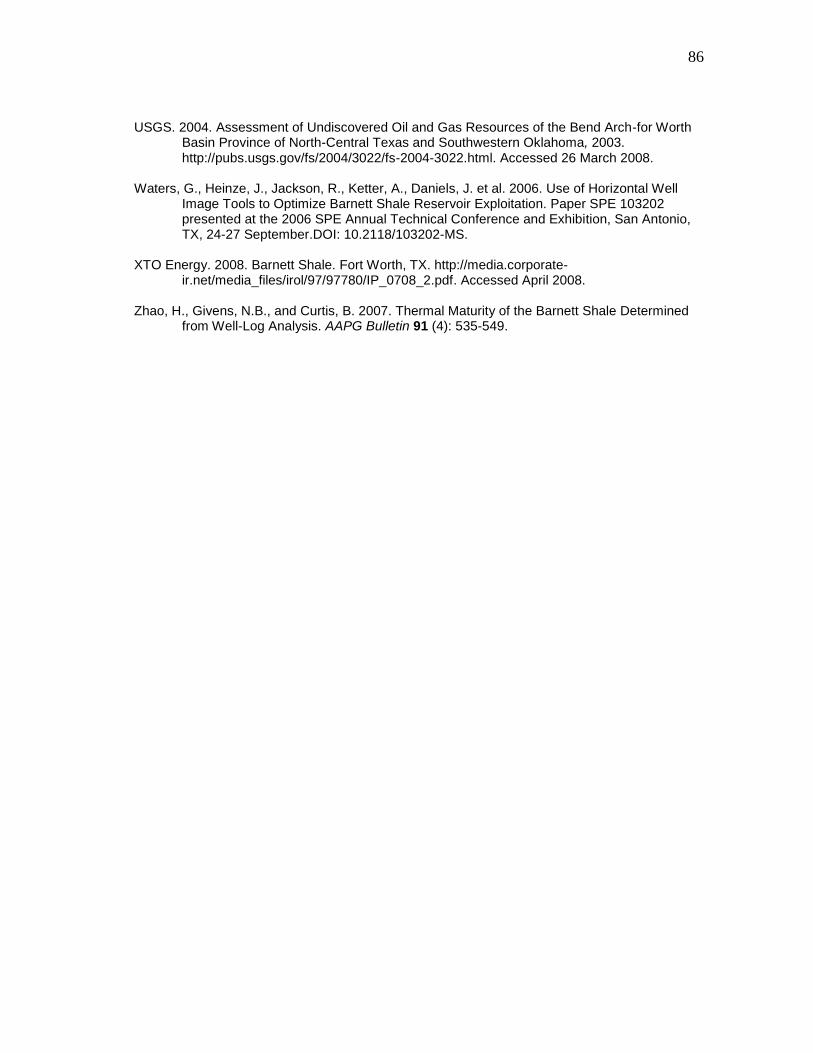
86
USGS. 2004. Assessment of Undiscovered Oil and Gas Resources of the Bend Arch-for Worth Basin Province of North-Central Texas and Southwestern Oklahoma, 2003. http://pubs.usgs.gov/fs/2004/3022/fs-2004-3022.html. Accessed 26 March 2008.
Waters, G., Heinze, J., Jackson, R., Ketter, A., Daniels, J. et al. 2006. Use of Horizontal Well
Image Tools to Optimize Barnett Shale Reservoir Exploitation. Paper SPE 103202 presented at the 2006 SPE Annual Technical Conference and Exhibition, San Antonio, TX, 24-27 September.DOI: 10.2118/103202-MS.
XTO Energy. 2008. Barnett Shale. Fort Worth, TX. http://media.corporate-
ir.net/media_files/irol/97/97780/IP_0708_2.pdf. Accessed April 2008. Zhao, H., Givens, N.B., and Curtis, B. 2007. Thermal Maturity of the Barnett Shale Determined
from Well-Log Analysis. AAPG Bulletin 91 (4): 535-549.
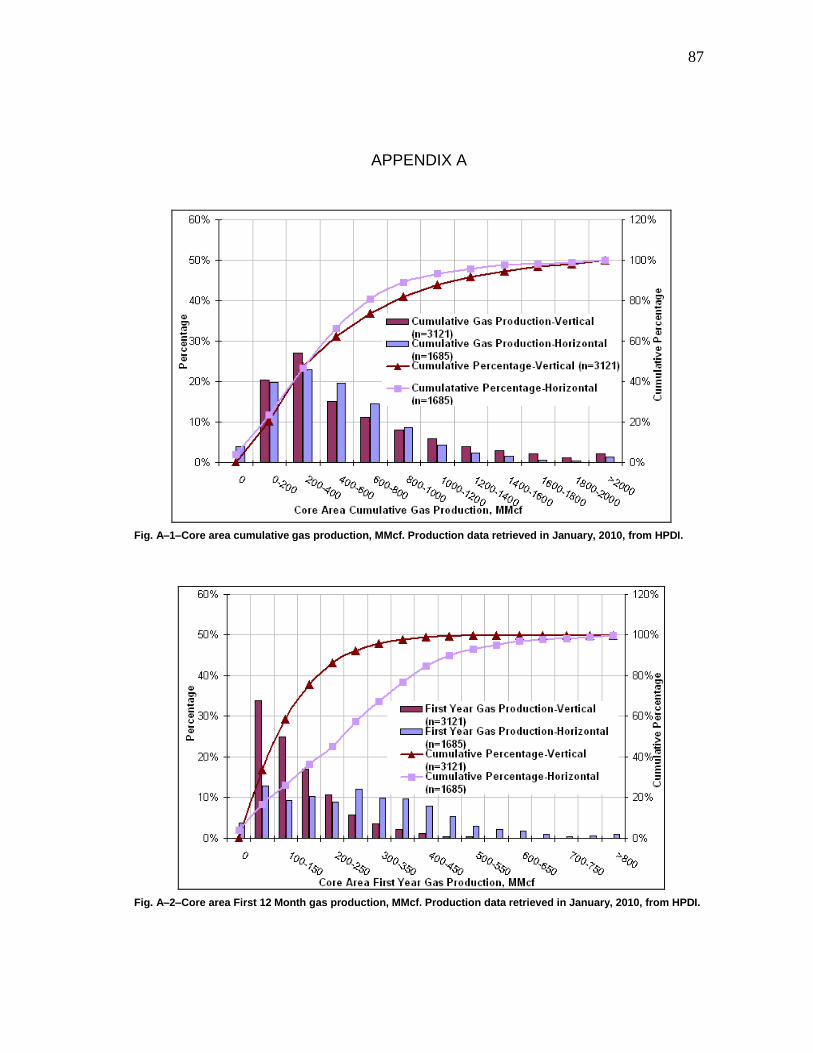
87
APPENDIX A
Fig. A–1–Core area cumulative gas production, MMcf. Production data retrieved in January, 2010, from HPDI.
Fig. A–2–Core area First 12 Month gas production, MMcf. Production data retrieved in January, 2010, from HPDI.
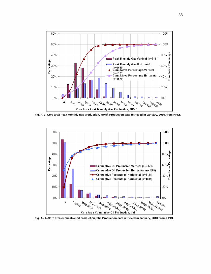
88
Fig. A–3–Core area Peak Monthly gas production, MMcf. Production data retrieved in January, 2010, from HPDI.
Fig. A– 4–Core area cumulative oil production, bbl. Production data retrieved in January, 2010, from HPDI.
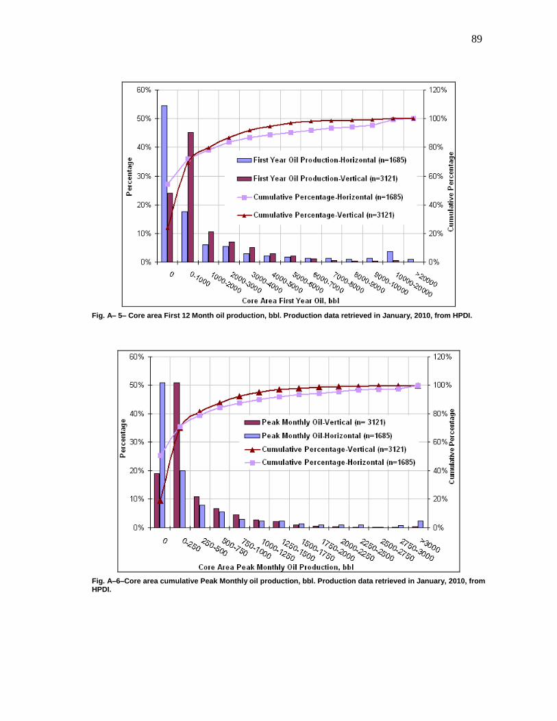
89
Fig. A– 5– Core area First 12 Month oil production, bbl. Production data retrieved in January, 2010, from HPDI.
Fig. A–6–Core area cumulative Peak Monthly oil production, bbl. Production data retrieved in January, 2010, from HPDI.
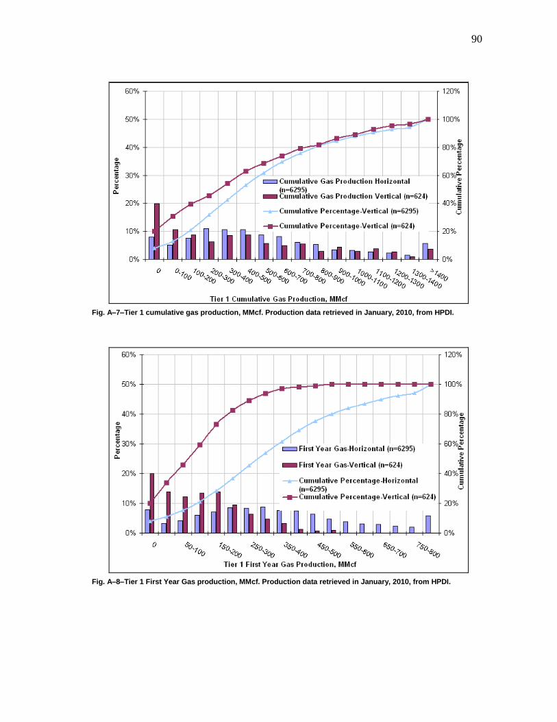
90
Fig. A–7–Tier 1 cumulative gas production, MMcf. Production data retrieved in January, 2010, from HPDI.
Fig. A–8–Tier 1 First Year Gas production, MMcf. Production data retrieved in January, 2010, from HPDI.
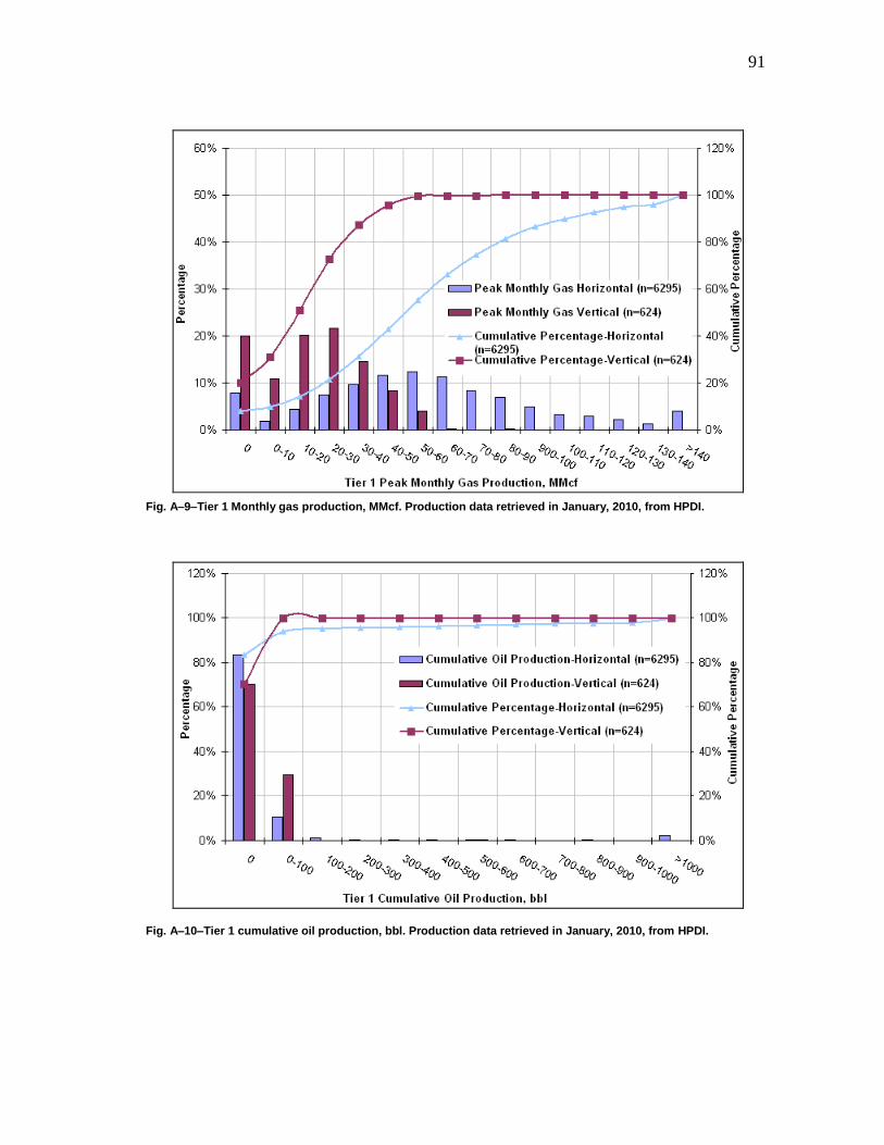
91
Fig. A–9–Tier 1 Monthly gas production, MMcf. Production data retrieved in January, 2010, from HPDI.
Fig. A–10–Tier 1 cumulative oil production, bbl. Production data retrieved in January, 2010, from HPDI.
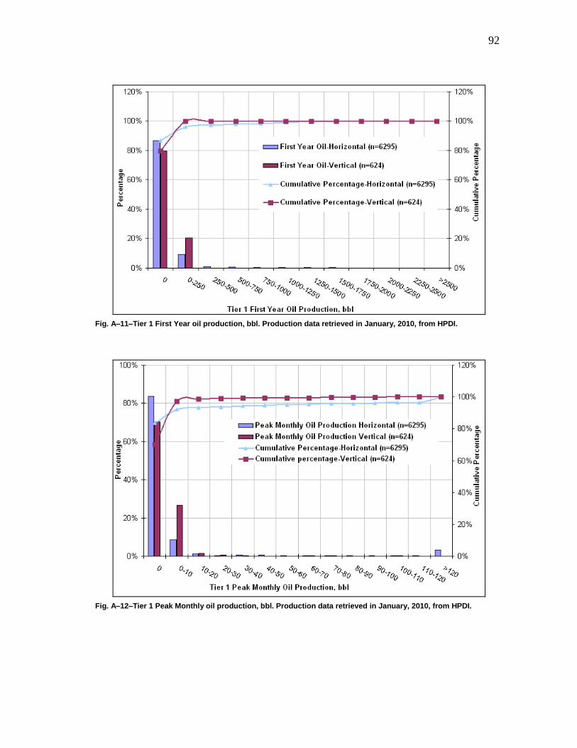
92
Fig. A–11–Tier 1 First Year oil production, bbl. Production data retrieved in January, 2010, from HPDI.
Fig. A–12–Tier 1 Peak Monthly oil production, bbl. Production data retrieved in January, 2010, from HPDI.
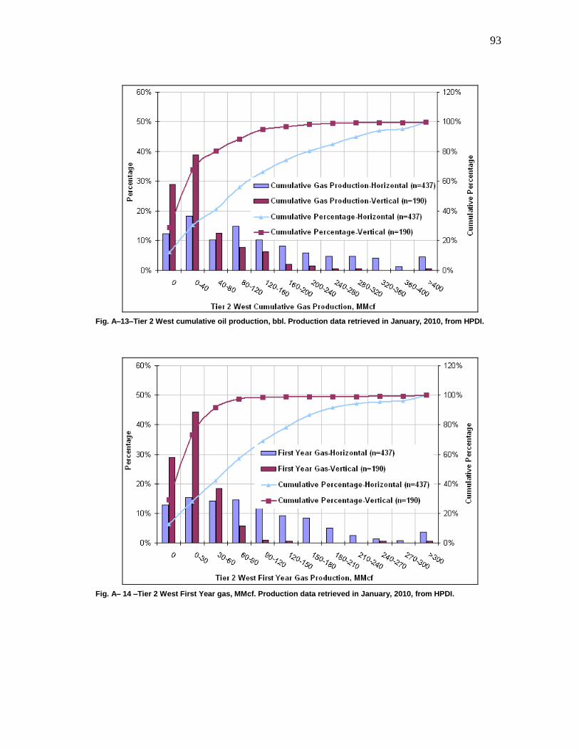
93
Fig. A–13–Tier 2 West cumulative oil production, bbl. Production data retrieved in January, 2010, from HPDI.
Fig. A– 14 –Tier 2 West First Year gas, MMcf. Production data retrieved in January, 2010, from HPDI.
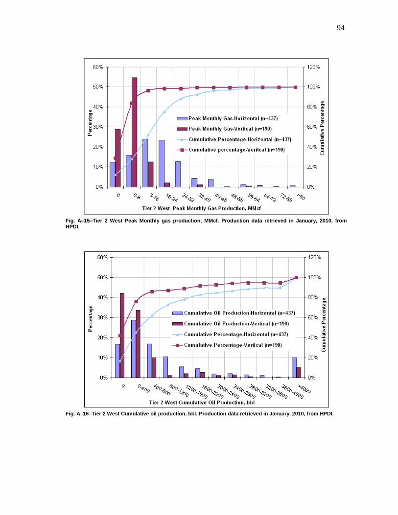
94
Fig. A–15–Tier 2 West Peak Monthly gas production, MMcf. Production data retrieved in January, 2010, from HPDI.
Fig. A–16–Tier 2 West Cumulative oil production, bbl. Production data retrieved in January, 2010, from HPDI.
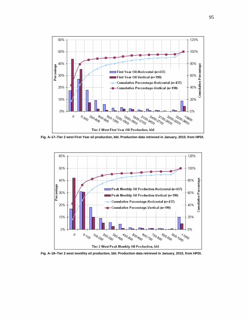
95
Fig. A–17–Tier 2 west First Year oil production, bbl. Production data retrieved in January, 2010, from HPDI.
Fig. A–18–Tier 2 west monthly oil production, bbl. Production data retrieved in January, 2010, from HPDI.
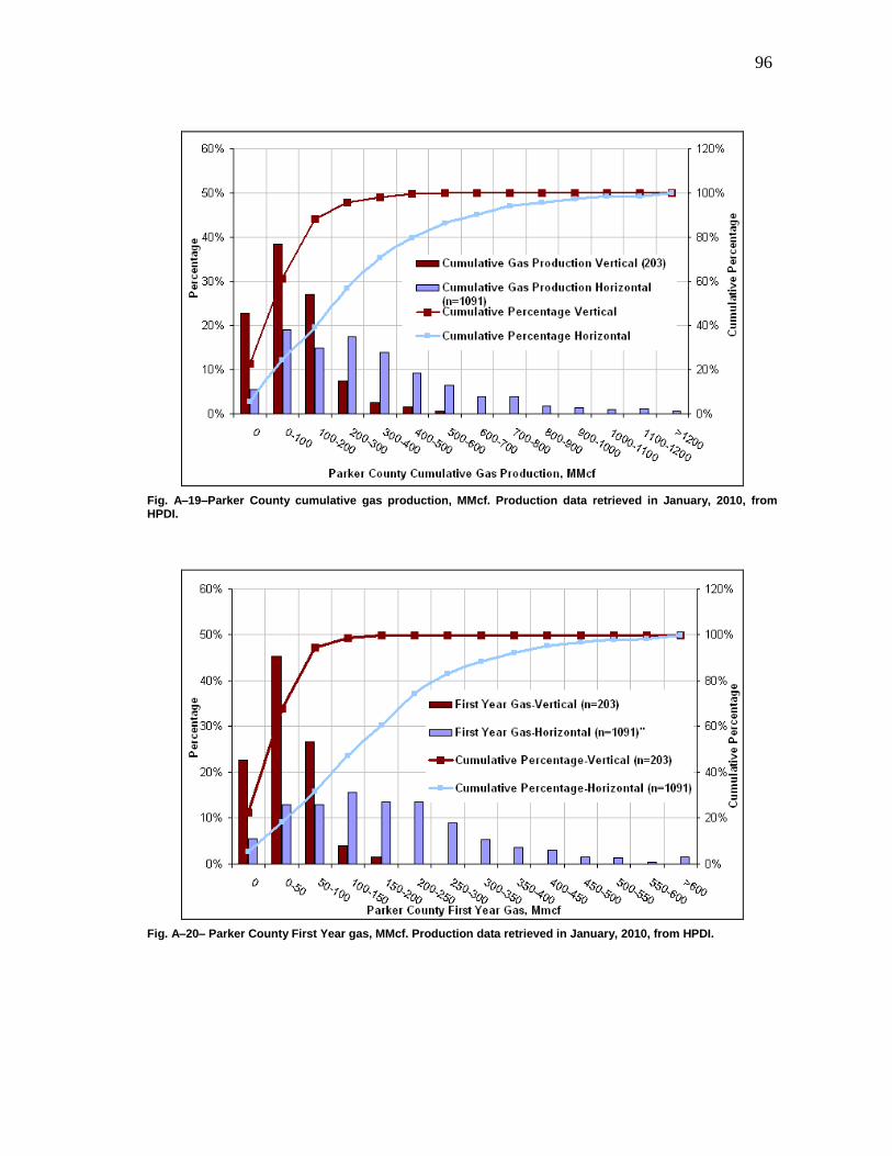
96
Fig. A–19–Parker County cumulative gas production, MMcf. Production data retrieved in January, 2010, from HPDI.
Fig. A–20– Parker County First Year gas, MMcf. Production data retrieved in January, 2010, from HPDI.
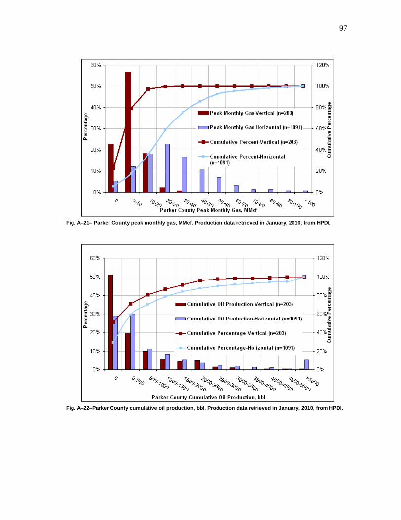
97
Fig. A–21– Parker County peak monthly gas, MMcf. Production data retrieved in January, 2010, from HPDI.
Fig. A–22–Parker County cumulative oil production, bbl. Production data retrieved in January, 2010, from HPDI.
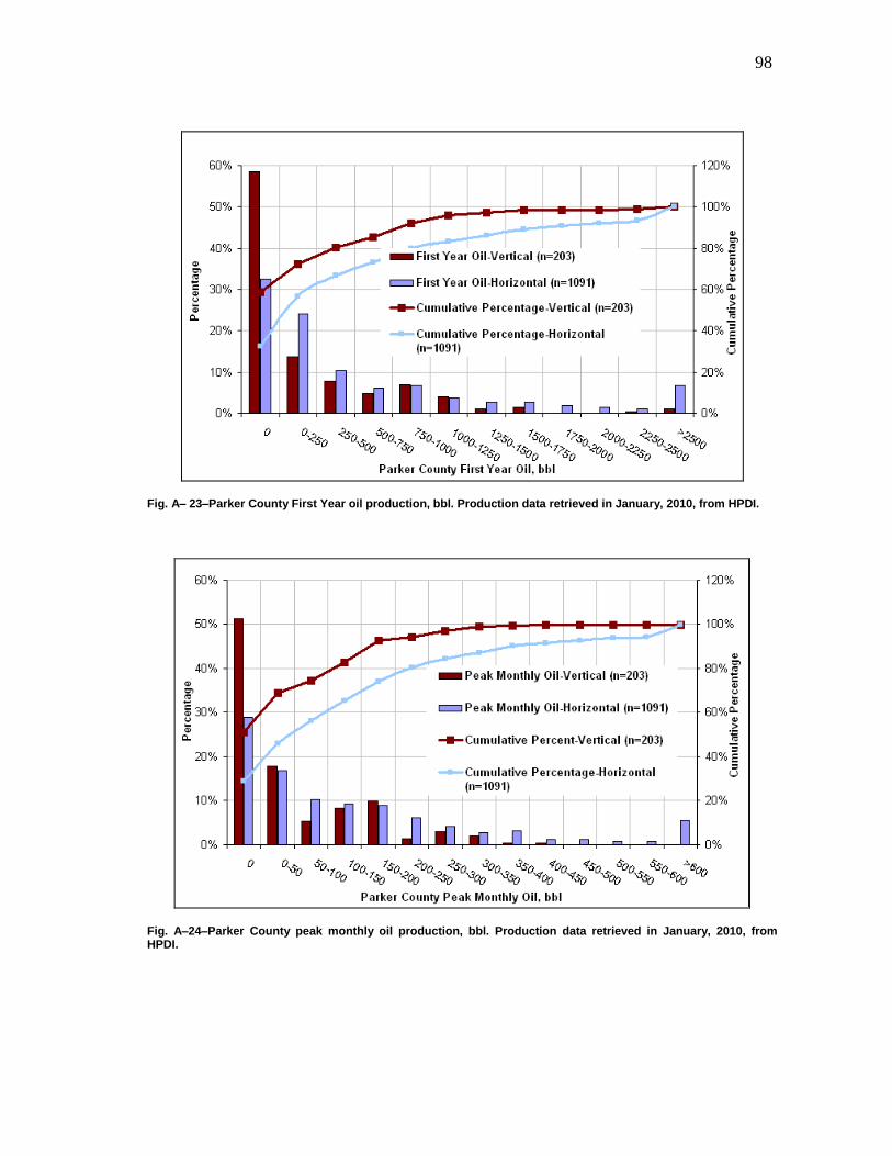
98
Fig. A– 23–Parker County First Year oil production, bbl. Production data retrieved in January, 2010, from HPDI.
Fig. A–24–Parker County peak monthly oil production, bbl. Production data retrieved in January, 2010, from HPDI.
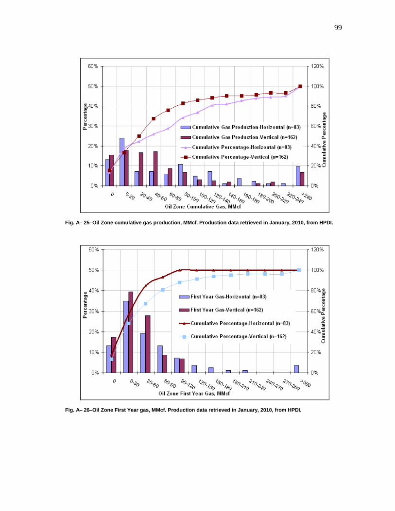
99
Fig. A– 25–Oil Zone cumulative gas production, MMcf. Production data retrieved in January, 2010, from HPDI.
Fig. A– 26–Oil Zone First Year gas, MMcf. Production data retrieved in January, 2010, from HPDI.
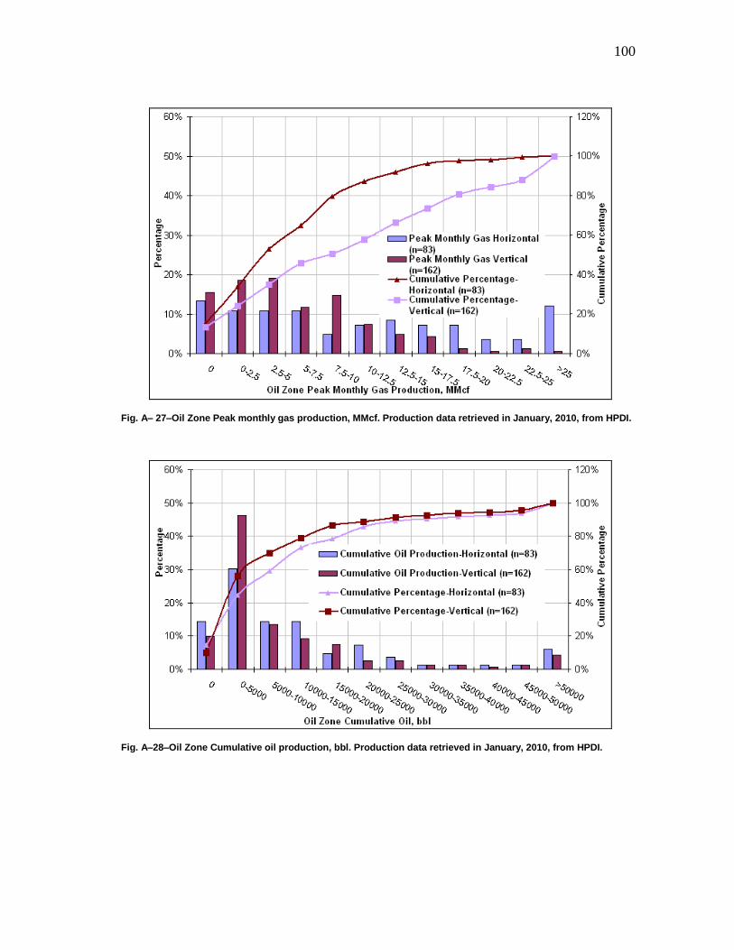
100
Fig. A– 27–Oil Zone Peak monthly gas production, MMcf. Production data retrieved in January, 2010, from HPDI.
Fig. A–28–Oil Zone Cumulative oil production, bbl. Production data retrieved in January, 2010, from HPDI.
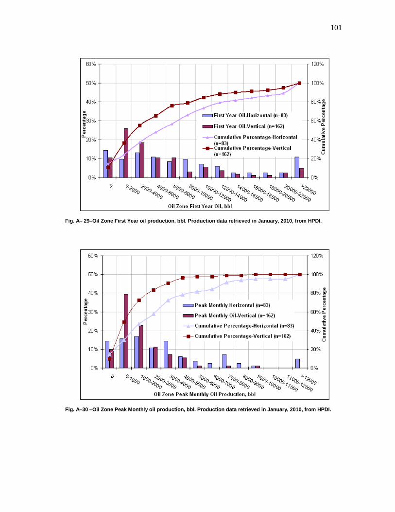
101
Fig. A– 29–Oil Zone First Year oil production, bbl. Production data retrieved in January, 2010, from HPDI.
Fig. A–30 –Oil Zone Peak Monthly oil production, bbl. Production data retrieved in January, 2010, from HPDI.

102
VITA
Yao Tian received her Bachelor of Science degree in petroleum engineering from China
University of Geosciences in 2007. She joined the Master of Science program in the Department
of Petroleum Engineering at Texas A&M University in the Fall of 2007.
Yao Tian may be reached at the Department of Petroleum Engineering, Texas A&M
University, TAMU 3116, College Station, TX 77843-3116.