An Improvement of Symbolic Aggregate Approximation

Distance Measure for Time Series

Youqiang Suna,c, Jiuyong Lib, Jixue Liub, Bingyu Suna,c, ChristopherChowd,e

aSchool of Information Science and Technology,University of Science and Technology of China, Hefei, Anhui, China

bSchool of Information Technology and Mathematical Sciences,University of South Australia, Adelaide, SA, Australia

cInstitute of Intelligent Machines, Chinese Academy of Sciences, Hefei, Anhui, ChinadAustralian Water Quality Centre, SA Water, Adelaide, SA, Australia

eSA Water Centre for Water Management and Reuse,University of South Australia, Adelaide, SA, Australia

Abstract

Symbolic Aggregate approXimation (SAX) as a major symbolic represen-tation has been widely used in many time series data mining applications.However, because a symbol is mapped from the average value of a segment,the SAX ignores important information in a segment, namely the trend ofthe value change in the segment. Such a miss may cause a wrong classifica-tion in some cases, since the SAX representation cannot distinguish differenttime series with similar average values but different trends. In this paper, wefirstly design a measure to compute the distance of trends using the startingand the ending points of segments. Then we propose a modified distancemeasure by integrating the SAX distance with a weighted trend distance.We show that our distance measure has a tighter lower bound to the Eu-clidean distance than that of the original SAX. The experimental results ondiverse time series data sets demonstrate that our proposed representationsignificantly outperforms the original SAX representation and an improvedSAX representation for classification.

Keywords: Time Series, Trend Distance, Symbolic AggregateApproximation, Lower Bound, Classification

Preprint submitted to Neurocomputing January 23, 2014

1. Introduction

Mining time series has attracted an increasing interest due to its wideapplications in finance, industry, medicine, biology, and so on. There are anumber of challenges in time series data mining, such as high dimensional-ity, high volumes, high feature correlation and large amount of noises. Inorder to reduce execution time and storage space, many high level represen-tations or abstractions of the raw time series data have been proposed. Thewell-known representations include Discrete Fourier Transform (DFT) [1],Discrete Wavelet Transform (DWT) [2], Discrete Cosine Transform (DCT)[3], Singular Value Decomposition (SVD) [4], Piecewise Aggregate Approxi-mation (PAA) [5] and Symbolic Aggregate approXimation (SAX) [6].

The SAX has become a major tool in time series data mining. TheSAX discretizes time series and reduces dimensionality/numerosity of data.The distance in the SAX representation has a lower bound to the Euclideandistance. In other words, the error between the distance in the SAX rep-resentation and the Euclidean distance in the original data is bounded [7].Therefore, the SAX representation speeds up the data mining process of timeseries data while maintaining the quality of the mining results. The SAXhas been widely used for applications in various domains such as mobile datamanagement [8], financial investment [9] and shape discovery [10].

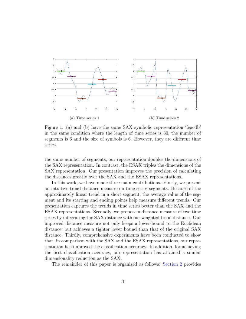
The SAX representation has a major limitation. In the SAX repre-sentation, symbols are mapped from the average values of segments. TheSAX representation does not consider the trends (or directions) in the seg-ments. Different segments with similar average values may be mapped tothe same symbols, and the SAX distance between them is 0. For example,in Fig. 1, time series (a) and (b) are different but their SAX representationsare the same as ’feacdb’. This drawback causes misclassifications when usingdistance-based classifiers.

The ESAX representation overcomes the above limitation by tripling thedimensions of the original SAX [11]. To distinguish the two time series inFig. 1, the ESAX representation adds additional symbols for the maximumand minimum points of a segment. The ESAX representations of time series(a) and (b) are ‘efffecaaaacffdbcbb’ and ‘effcefbaafcaadfbbc’ respectively.

We propose to store one value along with a symbol in the SAX to improvethe distance calculation of the SAX. Time series (a) and (b) in our representa-tion are represented as ‘0.2f1.2e−0.1a−1.2c1d−0.2b−0.3’ and ‘−0.3f−0.8e0a1.3c−1.4d0.4b0.3’respectively. Note that we store one additional value for the last segment. For

2

(a) Time series 1 (b) Time series 2

Figure 1: (a) and (b) have the same SAX symbolic representation ‘feacdb’in the same condition where the length of time series is 30, the number ofsegments is 6 and the size of symbols is 6. However, they are different timeseries.

the same number of segments, our representation doubles the dimensions ofthe SAX representation. In contrast, the ESAX triples the dimensions of theSAX representation. Our presentation improves the precision of calculatingthe distances greatly over the SAX and the ESAX representations.

In this work, we have made three main contributions. Firstly, we presentan intuitive trend distance measure on time series segments. Because of theapproximately linear trend in a short segment, the average value of the seg-ment and its starting and ending points help measure different trends. Ourpresentation captures the trends in time series better than the SAX and theESAX representations. Secondly, we propose a distance measure of two timeseries by integrating the SAX distance with our weighted trend distance. Ourimproved distance measure not only keeps a lower-bound to the Euclideandistance, but achieves a tighter lower bound than that of the original SAXdistance. Thirdly, comprehensive experiments have been conducted to showthat, in comparison with the SAX and the ESAX representations, our repre-sentation has improved the classification accuracy. In addition, for achievingthe best classification accuracy, our representation has attained a similardimensionality reduction as the SAX.

The remainder of this paper is organized as follows: Section 2 provides

3

the background knowledge of the SAX. Section 3 reviews the related work.Section 4 introduces our improved distance measure and its lower boundingproperty. Section 5 presents experimental evaluation on several time seriesdata sets. Finally, Section 6 concludes the paper and points out the futurework.

2. Background

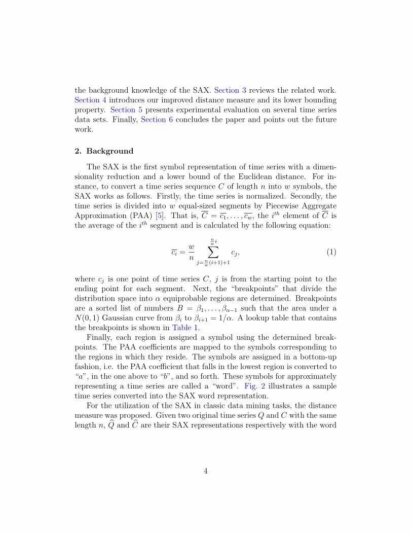
The SAX is the first symbol representation of time series with a dimen-sionality reduction and a lower bound of the Euclidean distance. For in-stance, to convert a time series sequence C of length n into w symbols, theSAX works as follows. Firstly, the time series is normalized. Secondly, thetime series is divided into w equal-sized segments by Piecewise AggregateApproximation (PAA) [5]. That is, C = c1, . . . , cw, the ith element of C isthe average of the ith segment and is calculated by the following equation:

ci =w

n

nwi∑

j= nw(i+1)+1

cj, (1)

where cj is one point of time series C, j is from the starting point to theending point for each segment. Next, the “breakpoints” that divide thedistribution space into α equiprobable regions are determined. Breakpointsare a sorted list of numbers B = β1, . . . , βα−1 such that the area under aN(0, 1) Gaussian curve from βi to βi+1 = 1/α. A lookup table that containsthe breakpoints is shown in Table 1.

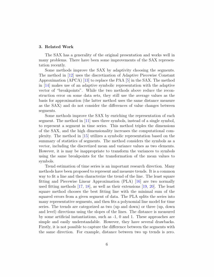
Finally, each region is assigned a symbol using the determined break-points. The PAA coefficients are mapped to the symbols corresponding tothe regions in which they reside. The symbols are assigned in a bottom-upfashion, i.e. the PAA coefficient that falls in the lowest region is converted to“a”, in the one above to “b”, and so forth. These symbols for approximatelyrepresenting a time series are called a “word”. Fig. 2 illustrates a sampletime series converted into the SAX word representation.

For the utilization of the SAX in classic data mining tasks, the distancemeasure was proposed. Given two original time series Q and C with the samelength n, Q and C are their SAX representations respectively with the word

4

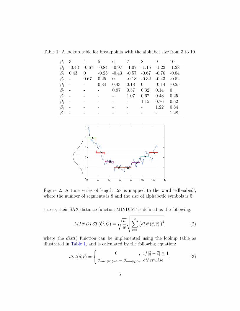
Table 1: A lookup table for breakpoints with the alphabet size from 3 to 10.

βi 3 4 5 6 7 8 9 10β1 -0.43 -0.67 -0.84 -0.97 -1.07 -1.15 -1.22 -1.28β2 0.43 0 -0.25 -0.43 -0.57 -0.67 -0.76 -0.84β3 - 0.67 0.25 0 -0.18 -0.32 -0.43 -0.52β4 - - 0.84 0.43 0.18 0 -0.14 -0.25β5 - - - 0.97 0.57 0.32 0.14 0β6 - - - - 1.07 0.67 0.43 0.25β7 - - - - - 1.15 0.76 0.52β8 - - - - - - 1.22 0.84β9 - - - - - - - 1.28

Figure 2: A time series of length 128 is mapped to the word ‘edbaabcd’,where the number of segments is 8 and the size of alphabetic symbols is 5.

size w, their SAX distance function MINDIST is defined as the following:

MINDIST (Q, C) =

√n

w

√√√√ w∑i=1

(dist (q, c)

)2, (2)

where the dist() function can be implemented using the lookup table asillustrated in Table 1, and is calculated by the following equation:

dist(q, c) =

{0 , if |q − c| ≤ 1

βmax(q,c)−1 − βmin(q,c), otherwise. (3)

5

3. Related Work

The SAX has a generality of the original presentation and works well inmany problems. There have been some improvements of the SAX represen-tation recently.

Some methods improve the SAX by adaptivity choosing the segments.The method in [12] uses the discretization of Adaptive Piecewise ConstantApproximation (APCA) [13] to replace the PAA [5] in the SAX. The methodin [14] makes use of an adaptive symbolic representation with the adaptivevector of “breakpoints”. While the two methods above reduce the recon-struction error on some data sets, they still use the average values as thebasis for approximation (the latter method uses the same distance measureas the SAX) and do not consider the differences of value changes betweensegments.

Some methods improve the SAX by enriching the representation of eachsegment. The method in [11] uses three symbols, instead of a single symbol,to represent a segment in time series. This method triples the dimensionsof the SAX, and the high dimensionality increases the computational com-plexity. The method in [15] utilizes a symbolic representation based on thesummary of statistics of segments. The method considers the symbols as avector, including the discretized mean and variance values as two elements.However, it is may be inappropriate to transform the variances to symbolsusing the same breakpoints for the transformation of the mean values tosymbols.

Trend estimation of time series is an important research direction. Manymethods have been proposed to represent and measure trends. It is a commonway to fit a line and then characterize the trend of the line. The least squarefitting and Piecewise Linear Approximation (PLA) [16] are two normallyused fitting methods [17, 18], as well as their extensions [19, 20]. The leastsquare method chooses the best fitting line with the minimal sum of thesquared errors from a given segment of data. The PLA splits the series intomany representative segments, and then fits a polynomial line model for timeseries. The trends are categorized as two (up and down) or three (up, downand level) directions using the slopes of the lines. The distance is measuredby some artificial instantiations, such as -1, 0 and 1. These approaches aresimple and easily understandable. However, they have several drawbacks.Firstly, it is not possible to capture the difference between the segments withthe same direction. For example, distance between two up trends is zero.

6

Secondly, there is not an appropriate measure to characterize the differenceof segments with different directions, such as the distance between “up”and “down” trends. Some other statistic approaches have been proposed in[21, 22, 23], but their models are complex.

4. SAX-TD: Improved SAX Based on Trend Distance

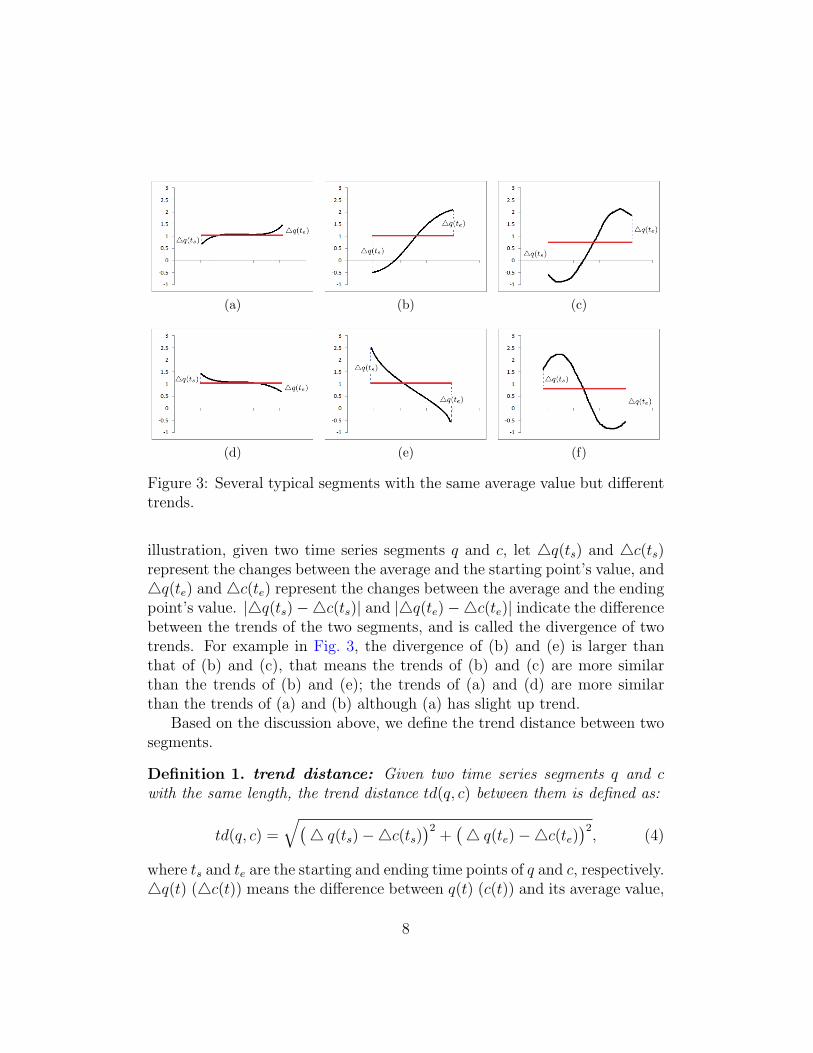
As we reviewed above, the time series segments are mapped to symbolsby their average values when using the SAX. This representation is imprecisewhen the trends of the segments are different but with similar average values.Fig. 3 lists several typical segments with the same average: (a) level and slightup, (b) obvious up, (c) down, up and then down, (d) level and slight down,(e) obvious down, (f) up, down and then up.

Trends are important characteristics of time series, and they are crucialfor the analysis of similarity and classification of time series [24]. Althoughthere are not a common definition of trend and a measurement of trenddistance in time series, the starting and the ending points are important insegment trend estimation. For example, a trend is up when the value of theending point is significant lager than the value of the starting point, whilethe trend is down when the value of the ending point is significant smallerthan the value of the starting point. It is difficult to qualitatively definea trend, such as the definitions of “significant up” and “significant down”,“significant down” and “slight down”. However, if the trend information of asegment is not utilized, the representations of a time series containing manysegments are rough.

In this paper, we do not use symbols to capture the trends of time series,but quantitatively measure the trends by calculating their distance, calledtrend distance. Because the divided segments are short, the trend in a seg-ment approximates a linear relationship in most of cases. Therefore, thestarting and the ending points approximatively determine a trend. Whenmore data points are used, the trend will be represented more precisely.However, the dimensions of the representation will be increased significantly.When we use the starting and the ending points, because of the continuityof time series data, only one extra dimension is added to one segment.

4.1. Distance Measures

We use the difference of changes between the average and the values ofstarting and ending points to quantify the distance of segments. For an

7

(a) (b) (c)

(d) (e) (f)

Figure 3: Several typical segments with the same average value but differenttrends.

illustration, given two time series segments q and c, let △q(ts) and △c(ts)represent the changes between the average and the starting point’s value, and△q(te) and △c(te) represent the changes between the average and the endingpoint’s value. |△q(ts)−△c(ts)| and |△q(te)−△c(te)| indicate the differencebetween the trends of the two segments, and is called the divergence of twotrends. For example in Fig. 3, the divergence of (b) and (e) is larger thanthat of (b) and (c), that means the trends of (b) and (c) are more similarthan the trends of (b) and (e); the trends of (a) and (d) are more similarthan the trends of (a) and (b) although (a) has slight up trend.

Based on the discussion above, we define the trend distance between twosegments.

Definition 1. trend distance: Given two time series segments q and cwith the same length, the trend distance td(q, c) between them is defined as:

td(q, c) =

√(△ q(ts)−△c(ts)

)2+(△ q(te)−△c(te)

)2, (4)

where ts and te are the starting and ending time points of q and c, respectively.△q(t) (△c(t)) means the difference between q(t) (c(t)) and its average value,

8

and can be calculated by:

△ q(t) = q(t)− q. (5)

The △c(t) is calculated in a similar way. Note that in Eq. (5), q is aknown value obtained by the PAA discretization, we just need to calculatethe △q(ts) and △q(te). We call △q(ts) and △q(te) as the trend variations ofa segment.

We incorporate the trend variations into the SAX representation. Becausethe continuity of time series data, the ending point of a segment is the startingpoint of the following segment. One segment needs only one trend variation(except the last segment). For an illustration, given two time series Q andC with the length of n, the representations with w words of them are:

Q : △q(1)q1△q(2)q2△q(3) . . .△q(w) qw△q(w+1),

C : △c(1)c1△c(2)c2△c(3) . . .△c(w) cw△c(w+1),

where q1, q2 . . . qw are the symbolic representations by the SAX,△q(1),△q(2). . .△q(w) are the trend variations, and △q(w + 1) is the change of the lastpoint. Compared to the original SAX, our representation adds w+1 dimen-sions for trend variations.

We define the distance between two time series based on the trend dis-tance as the following.

TDIST (Q, C) =

√n

w

√√√√ w∑i=1

((dist(qi, ci)

)2+

w

n

(td(qi, ci)

)2), (6)

where Q and C are the new representations of time series Q and C with thesame length n. w is the number of segments (or words), qi and ci are thesymbolic representations of segments qi and ci, respectively.

From Eq. (6), we see that the influence of the trend distance on theoverall distance is weighted by the ratio of dimensionality reduction w

n. w

nis

larger when there are more divided segments and each segment is shorter. wn

is smaller when there are fewer divided segments and each segment is longer.This is because in a short segment, the trend is likely to be linear and can belargely captured by two points and hence the weight for the trend distanceis high. When the segment is long, the trend is complex, two points areunlikely to capture the trend and hence the weight of the trend distance islow.

9

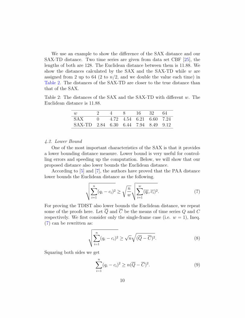
We use an example to show the difference of the SAX distance and ourSAX-TD distance. Two time series are given from data set CBF [25], thelengths of both are 128. The Euclidean distance between them is 11.88. Weshow the distances calculated by the SAX and the SAX-TD while w areassigned from 2 up to 64 (2 to n/2, and we double the value each time) inTable 2. The distances of the SAX-TD are closer to the true distance thanthat of the SAX.

Table 2: The distances of the SAX and the SAX-TD with different w. TheEuclidean distance is 11.88.

w 2 4 8 16 32 64SAX 0 4.72 4.54 6.21 6.60 7.24SAX-TD 2.84 6.30 6.44 7.94 8.49 9.12

4.2. Lower Bound

One of the most important characteristics of the SAX is that it providesa lower bounding distance measure. Lower bound is very useful for control-ling errors and speeding up the computation. Below, we will show that ourproposed distance also lower bounds the Euclidean distance.

According to [5] and [7], the authors have proved that the PAA distancelower bounds the Euclidean distance as the following.√√√√ n∑

i=1

(qi − ci)2 ≥√

n

w

√√√√ w∑i=1

(qi, ci)2. (7)

For proving the TDIST also lower bounds the Euclidean distance, we repeatsome of the proofs here. Let Q and C be the means of time series Q and Crespectively. We first consider only the single-frame case (i.e. w = 1), Ineq.(7) can be rewritten as:√√√√ n∑

i=1

(qi − ci)2 ≥√n

√(Q− C)2. (8)

Squaring both sides we get

n∑i=1

(qi − ci)2 ≥ n(Q− C)2. (9)

10

Recall that Q is the average of the time series, so qi can be represented interms of qi = Q−△qi. The same applies to each point ci in C. Thus, Ineq.(9) can be rewritten as the following.

n∑i=1

((Q−△qi)− (C −△ci)

)2 ≥ n(Q− C)2. (10)

Rearranging the left-hand side, we get

n∑i=1

((Q− C)− (△qi −△ci)

)2 ≥ n(Q− C)2. (11)

We can expand and then rewrite Ineq. (11) by the distributive law as thefollowing.

n∑i=1

(Q−C)2+n∑

i=1

(△qi−△ci)2−

n∑i=1

2(Q−C)(△qi−△ci) ≥ n(Q−C)2. (12)

Note that Q and C are independent to n, Ineq. (12) can be transformed asthe following.

n(Q−C)2+n∑

i=1

(△qi−△ci)2−2(Q−C)

n∑i=1

(△qi−△ci) ≥ n(Q−C)2. (13)

It was also proved that∑n

i=1(△qi −△ci) = 0 in [5]. Therefore, after substi-tuting 0 into the third term on the left-hand side, Ineq. (13) becomes:

n(Q− C)2 +n∑

i=1

(△qi −△ci)2 ≥ n(Q− C)2. (14)

Because∑n

i=1(△qi − △ci)2 ≥ 0, Ineq. (14) holds. Recall the definition in

(4),(td(q, c)

)2=

(△ q(ts)−△c(ts)

)2+(△ q(te)−△c(te)

)2, we can obtain

an inequality as the following (i = 1 is the starting point and i = n is theending point).

n∑i=1

(△qi −△ci)2 ≥ (△q1 −△c1)

2 + (△qn −△cn)2. (15)

11

Substituting Ineq. (15) into Ineq. (14), we get:

n(Q− C)2 +n∑

i=1

(△qi −△ci)2 ≥ n(Q− C)2 +

(td(qi, ci)

)2. (16)

According to [7], the MINDIST lower bounds the PAA distance, that is:

n(Q− C)2 ≥ n(dist(Q, C)

)2. (17)

where Q and C are symbolic representations of Q and C in the original SAX,respectively. By transitivity, the following inequality is true:

n(Q− C)2 +n∑

i=1

(△qi −△ci)2 ≥ n

(dist(Q, C)

)2+(td(qi, ci)

)2. (18)

Recall Ineq. (9), this means:

n∑i=1

(qi − ci)2 ≥ n

((dist(Q, C)

)2+

1

n

(td(qi, ci)

)2). (19)

N frames can be obtained by applying the single-frame proof on everyframe, that is:√√√√ n∑

i=1

(qi − ci)2 ≥√

n

w

√√√√ w∑i=1

((dist(qi, ci)

)2+

w

n

(td(qi, ci)

)2). (20)

The right-hand side of the above inequality is TDIST (Q,C) and the left-hand side is the Euclidean distance between Q and C. Therefore, the TDISTdistance lower bounds the Euclidean distance.

The quality of a lower bounding distance is usually measured by thetightness of lower bounding (TLB).

TLB =Lower Bounding Distance(Q,C)

Euclidean Distance(Q,C).

The value of TLB is in the range [0,1]. The larger the TLB value, the betterthe quality. Recall the distance measure in Eq. (6), we can obtain thatTLB (TDIST ) ≥ TLB (MINIDIST ), which means the SAX-TD distancehas a tighter lower bound than the original SAX distance.

In conclusion, our improved SAX-TD not only holds the lower boundingproperty of the original SAX, but also achieves a tighter lower bound.

12

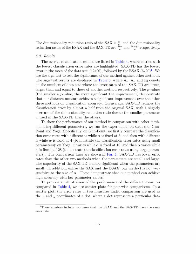
5. Experimental Validation

In this section, we will present the results of our experimental validation.Firstly we introduce the data sets used, the comparison methods and param-eter settings. Then we evaluate the performances of the proposed method interms of classification error rate, dimensionality reduction and efficiency.

5.1. Data sets

We performed the experiments on 20 diverse time series data sets, whichare provided by the UCR Time Series repository [25]. Some summary statis-tics of the data sets are given in Table 3. Each data set is divided into atraining set and a testing set. The data sets contain classes ranging from2 to 50, are of size from dozens to thousands, and have the lengths of timeseries varying from 60 to 637. In addition, the types of the data sets are alsodiverse, including synthetic, real (recorded from some processes) and shape(extracted by processing some shapes).

5.2. Comparison methods and parameter settings

Since our method aims to improve the SAX by modifying the distancemeasure, we do the evaluation on the classification task, of which the ac-curacy is determined by the distance measure. We compare the accuracieswith the classic Euclidean distance and the original SAX. To the best ofour knowledge, there is no other research improving the SAX distance bymeasuring trends. We choose an extension of SAX called as Extended SAX(ESAX) [11] to compare with. The ESAX adds two additional symbols forthe maximum and minimum values in a segment, but uses the same distancemeasure as the SAX after mapping. For example in Fig. 3, let us assume thatthe SAX words of sub-figure (b) and (e) are ‘b’, the ESAX representations ofthem are ‘abc’ and ‘cba’, respectively. Thus the distance calculated by theESAX is more accurate than that calculated by the SAX.

To compare the classification accuracy, we conduct the experiments us-ing 1 Nearest Neighbor (1-NN) classifier. The main advantage is that theunderlying distance metric is critical to the performance of 1-NN classifier,hence, the accuracy of the 1-NN classifier directly reflects the effectiveness ofa distance measure. Furthermore, 1-NN classifier is parameter free, allowingdirect comparisons of different measures.

To obtain the best accuracy for each method, we use the testing data tosearch for the best parameters w and α. For a given time series with length

13

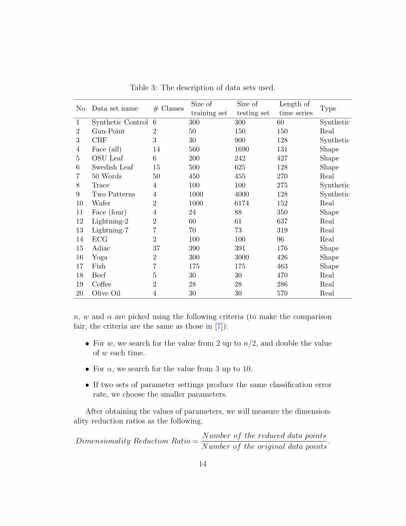
Table 3: The description of data sets used.

No. Data set name # ClassesSize oftraining set

Size oftesting set

Length oftime series

Type

1 Synthetic Control 6 300 300 60 Synthetic2 Gun-Point 2 50 150 150 Real3 CBF 3 30 900 128 Synthetic4 Face (all) 14 560 1690 131 Shape5 OSU Leaf 6 200 242 427 Shape6 Swedish Leaf 15 500 625 128 Shape7 50 Words 50 450 455 270 Real8 Trace 4 100 100 275 Synthetic9 Two Patterns 4 1000 4000 128 Synthetic10 Wafer 2 1000 6174 152 Real11 Face (four) 4 24 88 350 Shape12 Lightning-2 2 60 61 637 Real13 Lightning-7 7 70 73 319 Real14 ECG 2 100 100 96 Real15 Adiac 37 390 391 176 Shape16 Yoga 2 300 3000 426 Shape17 Fish 7 175 175 463 Shape18 Beef 5 30 30 470 Real19 Coffee 2 28 28 286 Real20 Olive Oil 4 30 30 570 Real

n, w and α are picked using the following criteria (to make the comparisonfair, the criteria are the same as those in [7]):

• For w, we search for the value from 2 up to n/2, and double the valueof w each time.

• For α, we search for the value from 3 up to 10.

• If two sets of parameter settings produce the same classification errorrate, we choose the smaller parameters.

After obtaining the values of parameters, we will measure the dimension-ality reduction ratios as the following.

Dimensionality Reduction Ratio =Number of the reduced data points

Number of the original data points.

14

The dimensionality reduction ratio of the SAX is wn, and the dimensionality

reduction ratios of the ESAX and the SAX-TD are 3∗wn

and 2∗w+1n

respectively.

5.3. Results

The overall classification results are listed in Table 4, where entries withthe lowest classification error rates are highlighted. SAX-TD has the lowesterror in the most of the data sets (12/20), followed by the ESAX (6/20)1. Weuse the sign test to test the significance of our method against other methods.The sign test results are displayed in Table 5, where n+, n− and n0 denoteon the numbers of data sets where the error rates of the SAX-TD are lower,larger than and equal to those of another method respectively. The p-values(the smaller a p-value, the more significant the improvement) demonstratethat our distance measure achieves a significant improvement over the otherthree methods on classification accuracy. On average, SAX-TD reduces theclassification error by almost a half from the original SAX, with a slightlydecrease of the dimensionality reduction ratio due to the smaller parameterw used in the SAX-TD than the others.

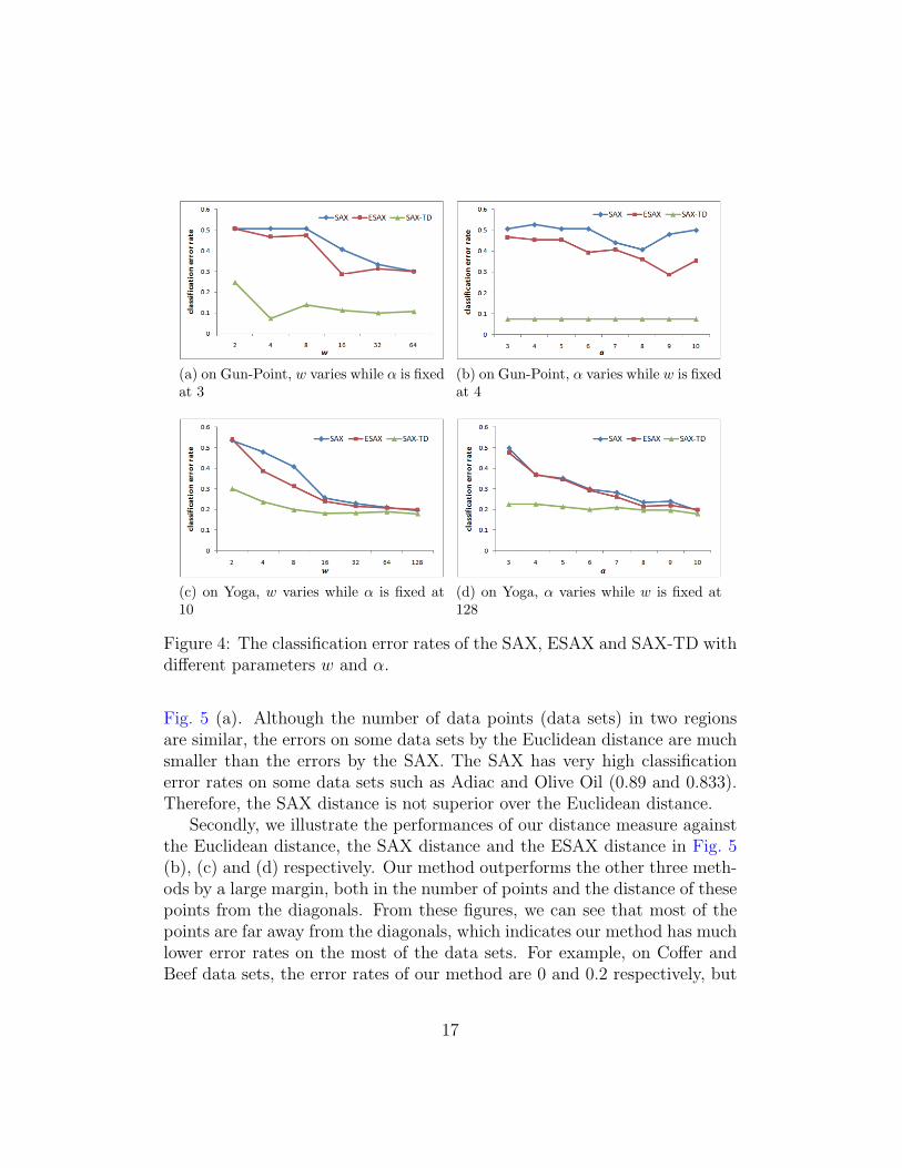
To show the performance of our method in comparison with other meth-ods using different parameters, we run the experiments on data sets Gun-Point and Yoga. Specifically, on Gun-Point, we firstly compare the classifica-tion error rates with different w while α is fixed at 3, and then with differentα while w is fixed at 4 (to illustrate the classification error rates using smallparameters); on Yoga, w varies while α is fixed at 10, and then α varies whilew is fixed at 128 (to illustrate the classification error rates using large param-eters). The comparison lines are shown in Fig. 4. SAX-TD has lower errorrates than the other two methods when the parameters are small and large.The superiority of the SAX-TD is more significant when the parameters aresmall. In addition, unlike the SAX and the ESAX, our method is not verysensitive to the size of α. These demonstrate that our method can achievehigh accuracy with low parameter values.

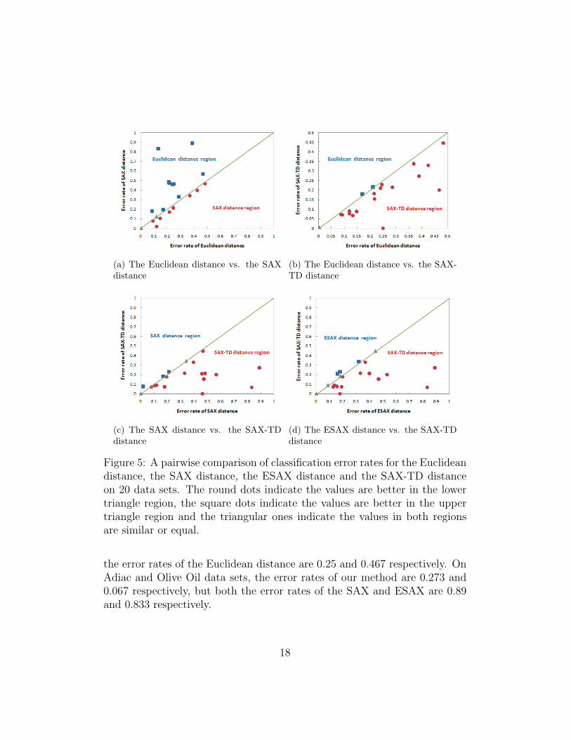
To provide an illustration of the performance of the different measurescompared in Table 4, we use scatter plots for pair-wise comparisons. In ascatter plot, the error rates of two measures under comparison are used asthe x and y coordinates of a dot, where a dot represents a particular data

1These numbers include two cases that the ESAX and the SAX-TD have the sameerror rate.

15

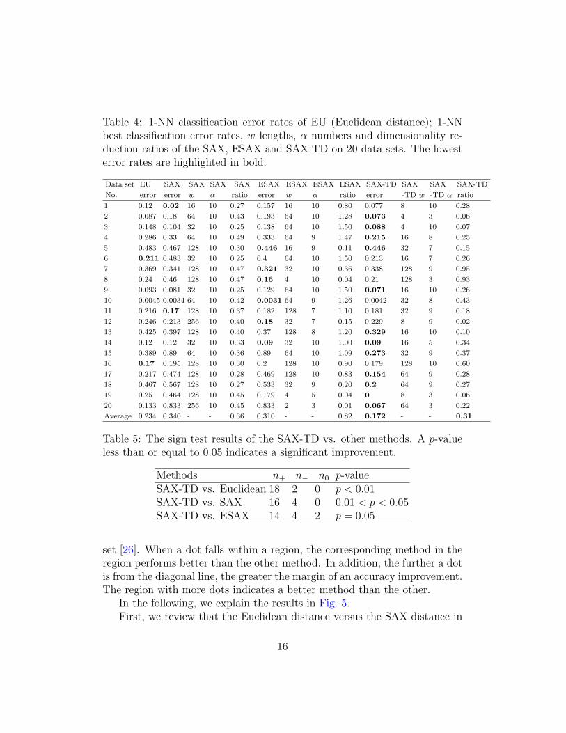
Table 4: 1-NN classification error rates of EU (Euclidean distance); 1-NNbest classification error rates, w lengths, α numbers and dimensionality re-duction ratios of the SAX, ESAX and SAX-TD on 20 data sets. The lowesterror rates are highlighted in bold.

Data set

No.

EU

error

SAX

error

SAX

w

SAX

α

SAX

ratio

ESAX

error

ESAX

w

ESAX

α

ESAX

ratio

SAX-TD

error

SAX

-TD w

SAX

-TD α

SAX-TD

ratio

1 0.12 0.02 16 10 0.27 0.157 16 10 0.80 0.077 8 10 0.28

2 0.087 0.18 64 10 0.43 0.193 64 10 1.28 0.073 4 3 0.06

3 0.148 0.104 32 10 0.25 0.138 64 10 1.50 0.088 4 10 0.07

4 0.286 0.33 64 10 0.49 0.333 64 9 1.47 0.215 16 8 0.25

5 0.483 0.467 128 10 0.30 0.446 16 9 0.11 0.446 32 7 0.15

6 0.211 0.483 32 10 0.25 0.4 64 10 1.50 0.213 16 7 0.26

7 0.369 0.341 128 10 0.47 0.321 32 10 0.36 0.338 128 9 0.95

8 0.24 0.46 128 10 0.47 0.16 4 10 0.04 0.21 128 3 0.93

9 0.093 0.081 32 10 0.25 0.129 64 10 1.50 0.071 16 10 0.26

10 0.0045 0.0034 64 10 0.42 0.0031 64 9 1.26 0.0042 32 8 0.43

11 0.216 0.17 128 10 0.37 0.182 128 7 1.10 0.181 32 9 0.18

12 0.246 0.213 256 10 0.40 0.18 32 7 0.15 0.229 8 9 0.02

13 0.425 0.397 128 10 0.40 0.37 128 8 1.20 0.329 16 10 0.10

14 0.12 0.12 32 10 0.33 0.09 32 10 1.00 0.09 16 5 0.34

15 0.389 0.89 64 10 0.36 0.89 64 10 1.09 0.273 32 9 0.37

16 0.17 0.195 128 10 0.30 0.2 128 10 0.90 0.179 128 10 0.60

17 0.217 0.474 128 10 0.28 0.469 128 10 0.83 0.154 64 9 0.28

18 0.467 0.567 128 10 0.27 0.533 32 9 0.20 0.2 64 9 0.27

19 0.25 0.464 128 10 0.45 0.179 4 5 0.04 0 8 3 0.06

20 0.133 0.833 256 10 0.45 0.833 2 3 0.01 0.067 64 3 0.22

Average 0.234 0.340 - - 0.36 0.310 - - 0.82 0.172 - - 0.31

Table 5: The sign test results of the SAX-TD vs. other methods. A p-valueless than or equal to 0.05 indicates a significant improvement.

Methods n+ n− n0 p-valueSAX-TD vs. Euclidean 18 2 0 p < 0.01SAX-TD vs. SAX 16 4 0 0.01 < p < 0.05SAX-TD vs. ESAX 14 4 2 p = 0.05

set [26]. When a dot falls within a region, the corresponding method in theregion performs better than the other method. In addition, the further a dotis from the diagonal line, the greater the margin of an accuracy improvement.The region with more dots indicates a better method than the other.

In the following, we explain the results in Fig. 5.First, we review that the Euclidean distance versus the SAX distance in

16

(a) on Gun-Point, w varies while α is fixedat 3

(b) on Gun-Point, α varies while w is fixedat 4

(c) on Yoga, w varies while α is fixed at10

(d) on Yoga, α varies while w is fixed at128

Figure 4: The classification error rates of the SAX, ESAX and SAX-TD withdifferent parameters w and α.

Fig. 5 (a). Although the number of data points (data sets) in two regionsare similar, the errors on some data sets by the Euclidean distance are muchsmaller than the errors by the SAX. The SAX has very high classificationerror rates on some data sets such as Adiac and Olive Oil (0.89 and 0.833).Therefore, the SAX distance is not superior over the Euclidean distance.

Secondly, we illustrate the performances of our distance measure againstthe Euclidean distance, the SAX distance and the ESAX distance in Fig. 5(b), (c) and (d) respectively. Our method outperforms the other three meth-ods by a large margin, both in the number of points and the distance of thesepoints from the diagonals. From these figures, we can see that most of thepoints are far away from the diagonals, which indicates our method has muchlower error rates on the most of the data sets. For example, on Coffer andBeef data sets, the error rates of our method are 0 and 0.2 respectively, but

17

(a) The Euclidean distance vs. the SAXdistance

(b) The Euclidean distance vs. the SAX-TD distance

(c) The SAX distance vs. the SAX-TDdistance

(d) The ESAX distance vs. the SAX-TDdistance

Figure 5: A pairwise comparison of classification error rates for the Euclideandistance, the SAX distance, the ESAX distance and the SAX-TD distanceon 20 data sets. The round dots indicate the values are better in the lowertriangle region, the square dots indicate the values are better in the uppertriangle region and the triangular ones indicate the values in both regionsare similar or equal.

the error rates of the Euclidean distance are 0.25 and 0.467 respectively. OnAdiac and Olive Oil data sets, the error rates of our method are 0.273 and0.067 respectively, but both the error rates of the SAX and ESAX are 0.89and 0.833 respectively.

18

5.4. Dimensionality reduction and efficiency

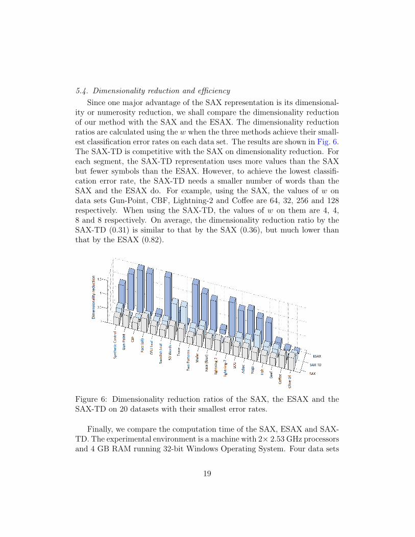
Since one major advantage of the SAX representation is its dimensional-ity or numerosity reduction, we shall compare the dimensionality reductionof our method with the SAX and the ESAX. The dimensionality reductionratios are calculated using the w when the three methods achieve their small-est classification error rates on each data set. The results are shown in Fig. 6.The SAX-TD is competitive with the SAX on dimensionality reduction. Foreach segment, the SAX-TD representation uses more values than the SAXbut fewer symbols than the ESAX. However, to achieve the lowest classifi-cation error rate, the SAX-TD needs a smaller number of words than theSAX and the ESAX do. For example, using the SAX, the values of w ondata sets Gun-Point, CBF, Lightning-2 and Coffee are 64, 32, 256 and 128respectively. When using the SAX-TD, the values of w on them are 4, 4,8 and 8 respectively. On average, the dimensionality reduction ratio by theSAX-TD (0.31) is similar to that by the SAX (0.36), but much lower thanthat by the ESAX (0.82).

Figure 6: Dimensionality reduction ratios of the SAX, the ESAX and theSAX-TD on 20 datasets with their smallest error rates.

Finally, we compare the computation time of the SAX, ESAX and SAX-TD. The experimental environment is a machine with 2× 2.53 GHz processorsand 4 GB RAM running 32-bit Windows Operating System. Four data sets

19

are used to show the running time with different w: Synthetic Control, ECG,CBF and Yoga. The maximum w values of the data sets are 16, 32, 64 and 128respectively. The α is fixed2 at the maximum value, i.e. 10. The results areshown in Fig. 7. Note that, the running time includes the transformation time(mapping values into words) and classification time (training and testing).We see that the running time increases with the increase of w. The SAX andthe SAX-TD take similar amount of time while the ESAX takes more timethan the both especially when w becomes larger. Since the SAX-TD needssmaller parameter w for achieving the best classification accuracy in mostcases, the computation time of SAX-TD is shorter than that of the SAX andESAX in many data sets.

6. Conclusions and Future Work

We have proposed an improved symbolic aggregate approximation dis-tance measure for time series. We firstly define a trend distance using thedivergences between the starting and ending points and the average. Wethen modify the original SAX distance measure by integrating a weightedtrend distance. The new distance measure keeps the important propertythat lower bounds the Euclidean distance. Furthermore, the lower bound ofour proposed measure is tighter than that of the original SAX. Accordingto the experimental results on diverse data sets, our improved measure de-creases the classification error rate significantly and needs a smaller numberof words and alphabetic symbols for achieving the best classification accu-racy than the SAX does. Our improved method has similar capability ofdimensionality reduction and has similar efficiency as the SAX.

For the future work, we intend to extend the method to other data min-ing tasks such as clustering, anomaly detection and motif discovery. Theproposed method may be utilized in improving the indexable Symbolic Ag-gregate approXimation (iSAX) [27] for terabyte sized time series.

Acknowledgment

This work has been partially supported by Australian Research CouncilDiscovery grant DP130104090 and the National Natural Science Foundation

2Since the efficiency is mainly determined by the value of parameter w, we just comparethe computation time with different w while α is fixed.

20

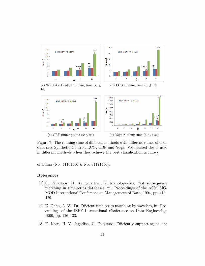
(a) Synthetic Control running time (w ≤16)

(b) ECG running time (w ≤ 32)

(c) CBF running time (w ≤ 64) (d) Yoga running time (w ≤ 128)

Figure 7: The running time of different methods with different values of w ondata sets Synthetic Control, ECG, CBF and Yoga. We marked the w usedin different methods when they achieve the best classification accuracy.

of China (No: 41101516 & No: 31171456).

References

[1] C. Faloutsos, M. Ranganathan, Y. Manolopoulos, Fast subsequencematching in time-series databases, in: Proceedings of the ACM SIG-MOD International Conference on Management of Data, 1994, pp. 419–429.

[2] K. Chan, A. W. Fu, Efficient time series matching by wavelets, in: Pro-ceedings of the IEEE International Conference on Data Engineering,1999, pp. 126–133.

[3] F. Korn, H. V. Jagadish, C. Faloutsos, Efficiently supporting ad hoc

21

queries in large datasets of time sequences, in: Proceedings of the ACMSIGMOD International Conference on Management of Data, 1997, pp.289–300.

[4] K. V. Ravi Kanth, D. Agrawal, A. Singh, Dimensionality reduction forsimilarity searching in dynamic databases, in: Proceedings of the ACMSIGMOD International Conference on Management of Data, 1998, pp.166–176.

[5] E. Keogh, K. Chakrabarti, M. Pazzani, S. Mehrotra, Dimensionality re-duction for fast similarity search in large time series databases, Knowl-edge and Information Systems 3 (3) (2001) 263–286.

[6] J. Lin, E. Keogh, S. Lonardi, B. Chiu, A symbolic representation oftime series, with implications for streaming algorithms, in: Proceedingsof the ACM SIGMOD Workshop on Research Issues in Data Mining andKnowledge Discovery, 2003, pp. 2–11.

[7] J. Lin, E. Keogh, L. Wei, S. Lonardi, Experiencing SAX: a novel sym-bolic representation of time series, Data Mining and Knowledge Discov-ery 15 (2) (2007) 107–144.

[8] H. Tayebi, S. Krishnaswamy, A. B. Waluyo, A. Sinha, M. M. Gaber,RA-SAX: Resource-aware symbolic aggregate approximation for mobileecg analysis, in: the IEEE International Conference on Mobile DataManagement, 2011, pp. 289–290.

[9] A. Canelas, R. Neves, N. Horta, A new SAX-GA methodology appliedto investment strategies optimization, in: Proceedings of the ACM In-ternational Conference on Genetic and Evolutionary Computation Con-ference, 2012, pp. 1055–1062.

[10] T. Rakthanmanon, E. Keogh, Fast shapelets: A scalable algorithm fordiscovering time series shapelets, in: Proceedings of the SIAM Confer-ence on Data Mining, 2013.

[11] B. Lkhagva, Y. Suzuki, K. Kawagoe, New time series data represen-tation esax for financial applications, in: the Workshops on the IEEEInternational Conference on Data Engineering, 2006, pp. x115–x115.

22

[12] B. Hugueney, Adaptive segmentation-based symbolic representations oftime series for better modeling and lower bounding distance measures,in: the European Conference on Principles and Practice of KnowledgeDiscovery in Databases, 2006, pp. 545–552.

[13] E. Keogh, K. Chakrabarti, M. Pazzani, S. Mehrotra, Locally adaptivedimensionality reduction for indexing large time series databases, in:Proceedings of the ACM SIGMOD International Conference on Man-agement of Data, 2001, pp. 151–162.

[14] N. D. Pham, Q. L. Le, T. K. Dang, Two novel adaptive symbolic rep-resentations for similarity search in time series databases, in: the IEEEInternational Asia-Pacific Web Conference, 2010, pp. 181–187.

[15] Z. X. Cai, Q. L. Zhong, The symbolic algorithm for time series databased on statistic feature, Chinese Journal of Computers 10 (2008) 1857–1864.

[16] H. Shatkay, S. B. Zdonik, Approximate queries and representations forlarge data sequences, in: Proceedings of the IEEE International Confer-ence on Data Engineering, 1996, pp. 536–545.

[17] P. Ljubic, L. Todorovski, N. Lavrac, J. C. Bullas, Time-series analysisof UK traffic accident data, in: Proceedings of the International Multi-conference Information Society, 2002, pp. 131–134.

[18] G. Z. Yu, H. Peng, Q. L. Zheng, Pattern distance of time series basedon segmentation by important points, in: Proceedings of the IEEE In-ternational Conference on Machine Learning and Cybernetics, Vol. 3,2005, pp. 1563–1567.

[19] M. Kontaki, A. N. Papadopoulos, Y. Manolopoulos, Continuous trend-based clustering in data streams, in: Proceedings of the InternationalConference on Data Warehousing and Knowledge Discovery, 2008, pp.251–262.

[20] M. Kontaki, A. N. Papadopoulos, Y. Manolopoulos, Continuous trend-based classification of streaming time series, in: Advances in Databasesand Information Systems, 2005, pp. 294–308.

23

[21] G. P. C. Fung, J. X. Yu, W. Lam, News sensitive stock trend prediction,in: Advances in Knowledge Discovery and Data Mining, 2002, pp. 481–493.

[22] H. Wu, B. Salzberg, D. Zhang, Online event-driven subsequence match-ing over financial data streams, in: Proceedings of the ACM SIGMODInternational Conference on Management of Data, 2004, pp. 23–34.

[23] W. B. Wu, Z. Zhao, Inference of trends in time series, Journal of theRoyal Statistical Society: Series B (Statistical Methodology) 69 (3)(2007) 391–410.

[24] T.-c. Fu, A review on time series data mining, Engineering Applicationsof Artificial Intelligence 24 (1) (2011) 164–181.

[25] E. Keogh, Q. Zhu, B. Hu, Y. Hao, X. Xi, L. Wei, C. A. Ratanamahatana,The UCR time series classification/clustering homepage, http://www.cs.ucr.edu/~eamonn/time_series_data/ (2011).

[26] H. Ding, G. Trajcevski, P. Scheuermann, X. Wang, E. Keogh, Queryingand mining of time series data: experimental comparison of represen-tations and distance measures, Proceedings of the VLDB Endowment1 (2) (2008) 1542–1552.

[27] J. Shieh, E. Keogh, iSAX: indexing and mining terabyte sized timeseries, in: Proceedings of the ACM SIGKDD International Conferenceon Knowledge Discovery and Data Mining, 2008, pp. 623–631.

24