Embed Size (px)
Citation preview
Symbolic Model Reductionfor Linear and Nonlinear DAEs
Symposium on Recent Advances in MORTU Eindhoven, The NetherlandsNovember 23rd, 2007
Thomas [email protected]
Slide 2
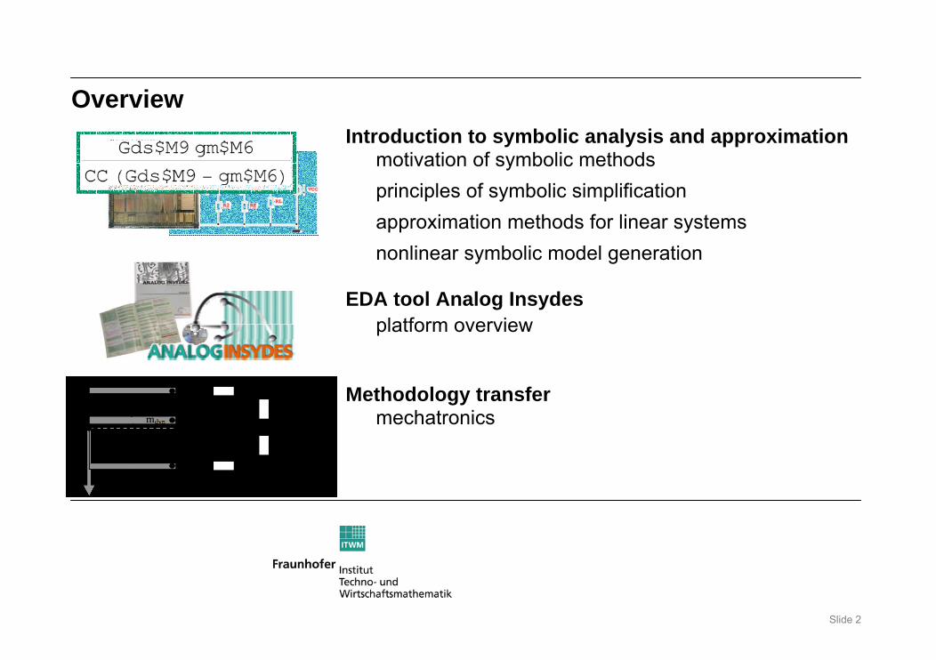
Introduction to symbolic analysis and approximationmotivation of symbolic methodsprinciples of symbolic simplificationapproximation methods for linear systemsnonlinear symbolic model generation
EDA tool Analog Insydes
Overview
platform overview
Methodology transfermechatronics
Slide 3
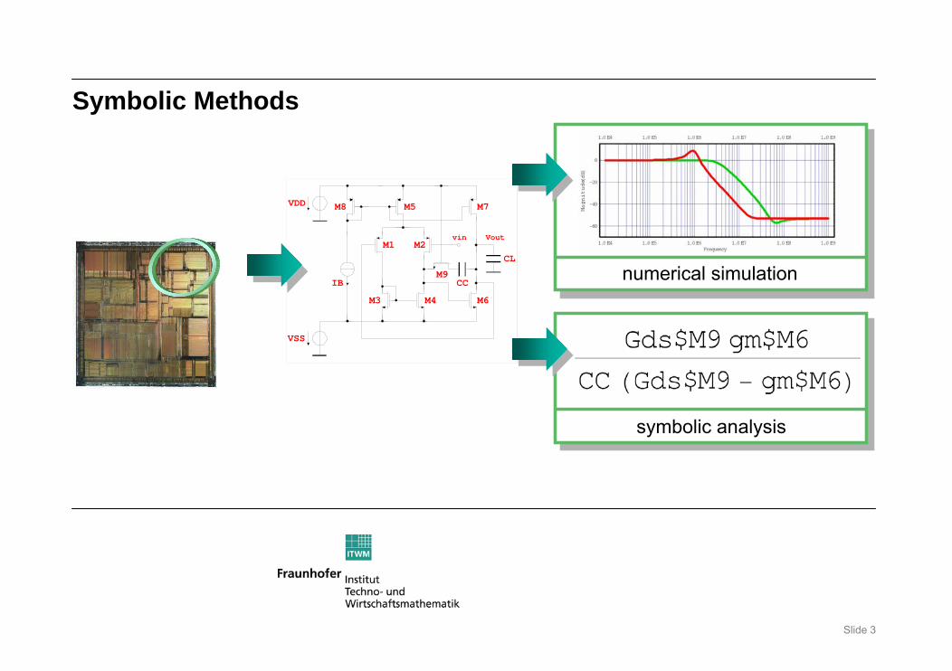
Symbolic Methods
M1
M3
IB
M4 M6
M5 M7
M2
M8VDD
VSS
vin Vout
CC
CL
M9 numerical simulation
symbolic analysis
Slide 4
A=1A=1Loop filter
F(s)Loop filter
F(s)
VCOVCO
ff ii
ff oo
Ctrl. logicCtrl. logic
Phasecomparator
Phasecomparator
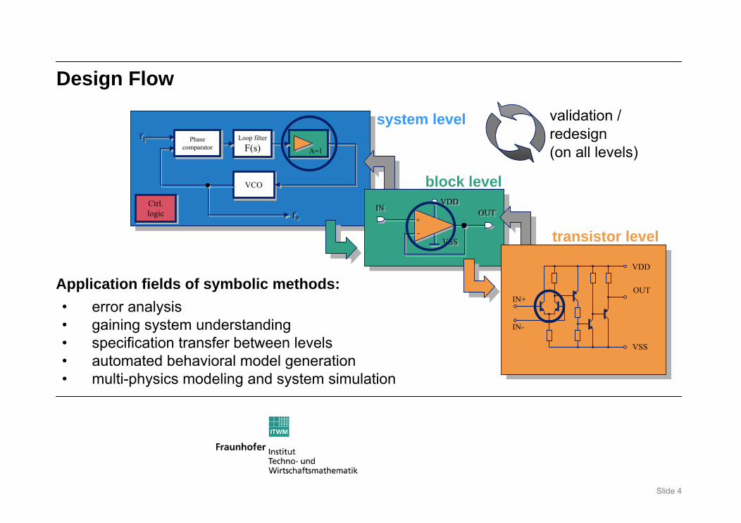
Design Flow
system level
block level
transistor level
• error analysis• gaining system understanding• specification transfer between levels• automated behavioral model generation• multi-physics modeling and system simulation
validation / redesign(on all levels)
++
--
VDDVDD
VSSVSS
ININOUTOUT
VDD
VSS
OUTIN+
IN-
Application fields of symbolic methods:
Slide 5
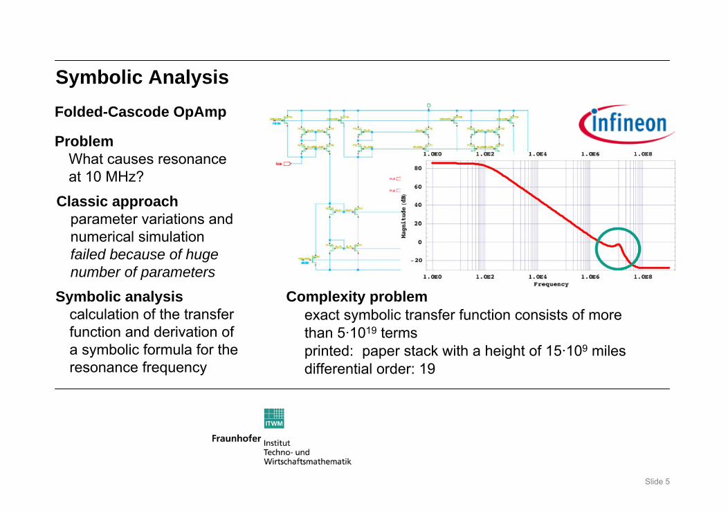
Folded-Cascode OpAmp
ProblemWhat causes resonanceat 10 MHz?
Classic approachparameter variations and numerical simulationfailed because of hugenumber of parameters
Symbolic analysiscalculation of the transferfunction and derivation ofa symbolic formula for theresonance frequency
Complexity problem
Symbolic Analysis
exact symbolic transfer function consists of more than 5·1019 termsprinted: paper stack with a height of 15·109 milesdifferential order: 19
Slide 6
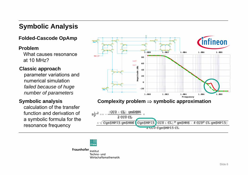
Folded-Cascode OpAmp
ProblemWhat causes resonanceat 10 MHz?
Classic approachparameter variations and numerical simulationfailed because of hugenumber of parameters
Symbolic Analysis
Symbolic analysiscalculation of the transferfunction and derivation ofa symbolic formula for theresonance frequency
Complexity problem ⇒ symbolic approximation
Slide 7
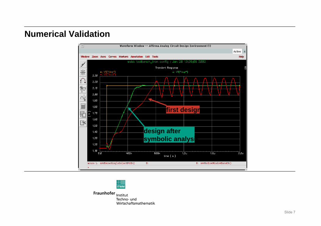
Numerical Validation
first design
design aftersymbolic analysis
Slide 8
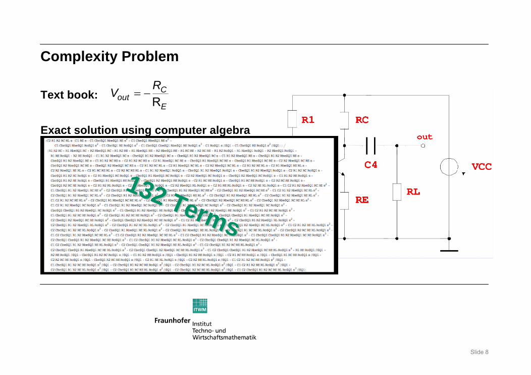
Text book:
Complexity Problem
Exact solution using computer algebra
132 Terms
132 Terms
= −R
Cout
E
RV
Slide 9
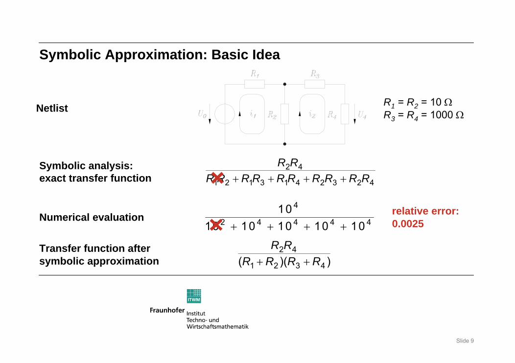
Symbolic analysis:exact transfer function
Netlist
Symbolic Approximation: Basic Idea
+ + + +2 4
1 2 1 3 1 4 2 3 2 4
R RR R R R R R R R R R
R1 = R2 = 10 ΩR3 = R4 = 1000 Ω
+ + + +
4
2 4 4 4 410
10 10 10 10 10Numerical evaluation
+ +2 4
1 2 3 4( )( )R R
R R R RTransfer function aftersymbolic approximation
relative error:0.0025
Slide 10
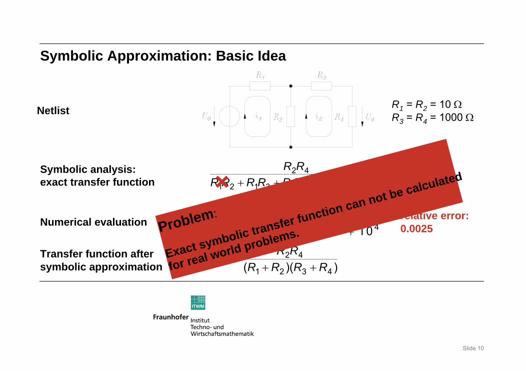
Symbolic analysis:exact transfer function
Netlist
Symbolic Approximation: Basic Idea
+ + + +2 4
1 2 1 3 1 4 2 3 2 4
R RR R R R R R R R R R
R1 = R2 = 10 ΩR3 = R4 = 1000 Ω
+ + + +
4
2 4 4 4 410
10 10 10 10 10Numerical evaluation
+ +2 4
1 2 3 4( )( )R R
R R R RTransfer function aftersymbolic approximation
relative error:0.0025Problem:
Exact symbolic transfer function can not be calculated
for real world problems.
Slide 11
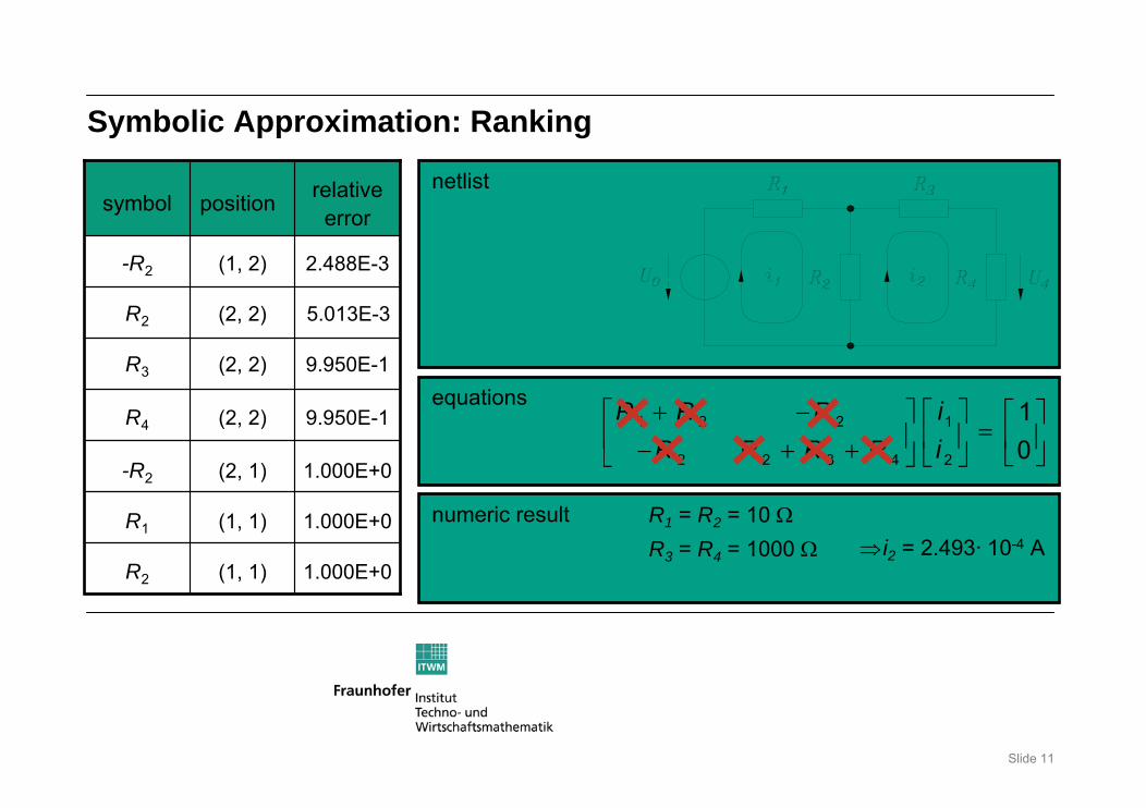
Symbolic Approximation: Ranking
equations + −⎡ ⎤ ⎡ ⎤ ⎡ ⎤=⎢ ⎥ ⎢ ⎥ ⎢ ⎥− + + ⎣ ⎦⎣ ⎦⎣ ⎦
1 2 2 1
2 2 3 4 2
10
R R R iR R R R i
netlist
numeric result R1 = R2 = 10 ΩR3 = R4 = 1000 Ω ⇒ i2 = 2.493· 10-4 A
relative error
positionsymbol
1.000E+0(1, 1)R2
1.000E+0(1, 1)R1
1.000E+0(2, 1)-R2
9.950E-1(2, 2)R4
9.950E-1(2, 2)R3
5.013E-3(2, 2)R2
2.488E-3(1, 2)-R2
Slide 12
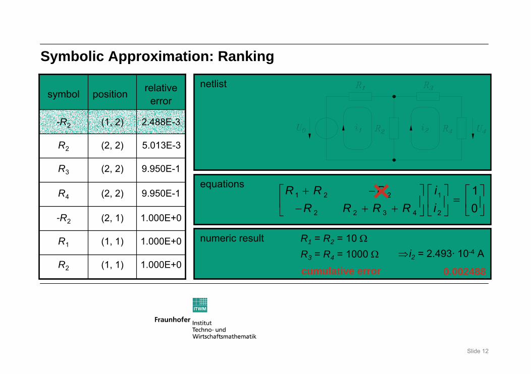
Symbolic Approximation: Ranking
equations + −⎡ ⎤ ⎡ ⎤ ⎡ ⎤=⎢ ⎥ ⎢ ⎥ ⎢ ⎥− + + ⎣ ⎦⎣ ⎦⎣ ⎦
1 2 2 1
2 2 3 4 2
10
R R R iR R R R i
netlist
numeric result R1 = R2 = 10 ΩR3 = R4 = 1000 Ω ⇒ i2 = 2.493· 10-4 A
relative error
positionsymbol
1.000E+0(1, 1)R2
1.000E+0(1, 1)R1
1.000E+0(2, 1)-R2
9.950E-1(2, 2)R4
9.950E-1(2, 2)R3
5.013E-3(2, 2)R2
2.488E-3(1, 2)-R2
cumulative error 0.002488

Slide 13
Symbolic Approximation: Ranking
equations + −⎡ ⎤ ⎡ ⎤ ⎡ ⎤=⎢ ⎥ ⎢ ⎥ ⎢ ⎥− + + ⎣ ⎦⎣ ⎦⎣ ⎦
1 2 2 1
2 2 3 4 2
10
R R R iR R R R i
netlist
numeric result R1 = R2 = 10 ΩR3 = R4 = 1000 Ω ⇒ i2 = 2.493· 10-4 A
relative error
positionsymbol
1.000E+0(1, 1)R2
1.000E+0(1, 1)R1
1.000E+0(2, 1)-R2
9.950E-1(2, 2)R4
9.950E-1(2, 2)R3
5.013E-3(2, 2)R2
2.488E-3(1, 2)-R2
cumulative error 0.0025
Slide 14
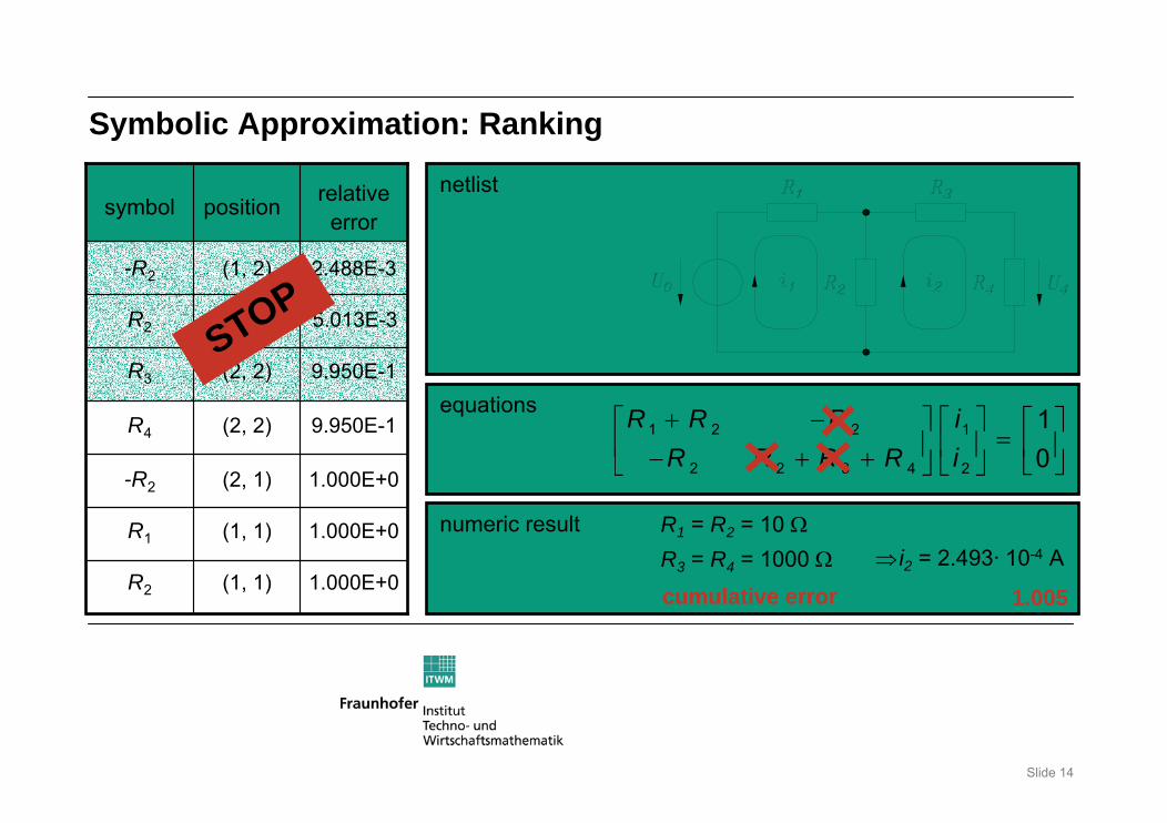
Symbolic Approximation: Ranking
equations + −⎡ ⎤ ⎡ ⎤ ⎡ ⎤=⎢ ⎥ ⎢ ⎥ ⎢ ⎥− + + ⎣ ⎦⎣ ⎦⎣ ⎦
1 2 2 1
2 2 3 4 2
10
R R R iR R R R i
netlist
numeric result R1 = R2 = 10 ΩR3 = R4 = 1000 Ω ⇒ i2 = 2.493· 10-4 A
relative error
positionsymbol
1.000E+0(1, 1)R2
1.000E+0(1, 1)R1
1.000E+0(2, 1)-R2
9.950E-1(2, 2)R4
9.950E-1(2, 2)R3
5.013E-3(2, 2)R2
2.488E-3(1, 2)-R2
cumulative error 1.005
STOP
Slide 15
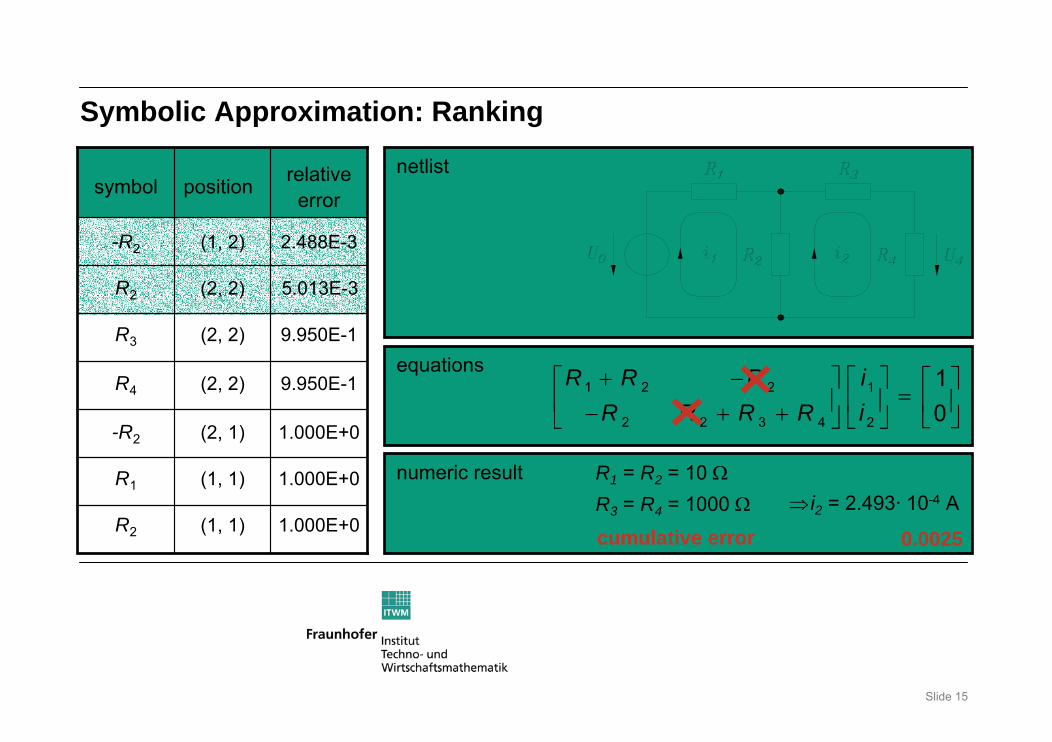
Symbolic Approximation: Ranking
equations + −⎡ ⎤ ⎡ ⎤ ⎡ ⎤=⎢ ⎥ ⎢ ⎥ ⎢ ⎥− + + ⎣ ⎦⎣ ⎦⎣ ⎦
1 2 2 1
2 2 3 4 2
10
R R R iR R R R i
netlist
numeric result R1 = R2 = 10 ΩR3 = R4 = 1000 Ω ⇒ i2 = 2.493· 10-4 A
relative error
positionsymbol
1.000E+0(1, 1)R2
1.000E+0(1, 1)R1
1.000E+0(2, 1)-R2
9.950E-1(2, 2)R4
9.950E-1(2, 2)R3
5.013E-3(2, 2)R2
2.488E-3(1, 2)-R2
cumulative error 0.0025
Slide 16
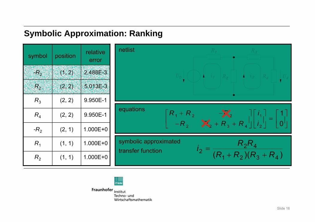
Symbolic Approximation: Ranking
netlist
symbolic approximatedtransfer function
relative error
positionsymbol
1.000E+0(1, 1)R2
1.000E+0(1, 1)R1
1.000E+0(2, 1)-R2
9.950E-1(2, 2)R4
9.950E-1(2, 2)R3
5.013E-3(2, 2)R2
2.488E-3(1, 2)-R2
=+ +
2 42
1 2 3 4( )( )R Ri
R R R R
equations + −⎡ ⎤ ⎡ ⎤ ⎡ ⎤=⎢ ⎥ ⎢ ⎥ ⎢ ⎥− + + ⎣ ⎦⎣ ⎦⎣ ⎦
1 2 2 1
2 2 3 4 2
10
R R R iR R R R i
Slide 17
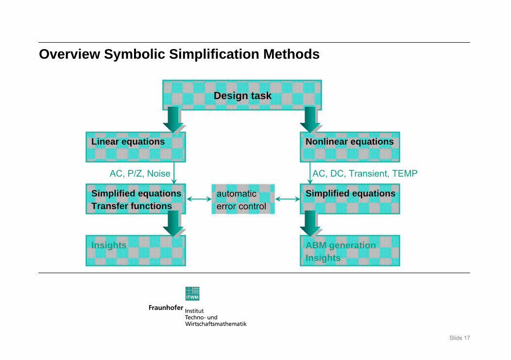
Overview Symbolic Simplification Methods
Simplified equationsTransfer functions
Simplified equationsautomaticerror control
Nonlinear equationsLinear equations
Insights ABM generationInsights
Design task
AC, P/Z, Noise AC, DC, Transient, TEMP
Slide 18
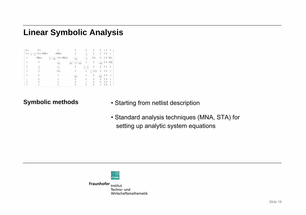
Linear Symbolic Analysis
• Starting from netlist descriptionSymbolic methods
• Standard analysis techniques (MNA, STA) forsetting up analytic system equations
Slide 19
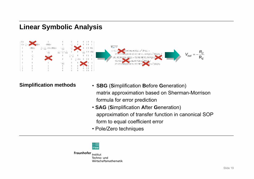
Linear Symbolic Analysis
• SBG (Simplification Before Generation)matrix approximation based on Sherman-Morrison formula for error prediction
Simplification methods
= −R
Cout
E
RV
• SAG (Simplification After Generation)approximation of transfer function in canonical SOPform to equal coefficient error
• Pole/Zero techniques
Slide 20
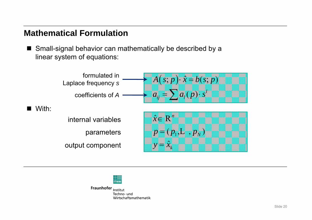
Mathematical Formulation
Small-signal behavior can mathematically be described by alinear system of equations:
( ) ˆ; ( ; )
( ) lij l
A s p x b s p
a a p s
⋅ =
= ⋅∑
formulated inLaplace frequency s
coefficients of A
1
ˆ( , , )ˆ
n
N
k
xp p py x
∈=
=
LR
With:internal variables
parameters
output component
Slide 21
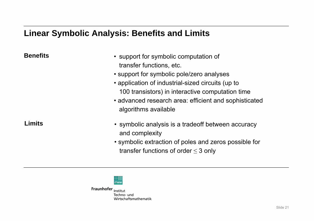
Linear Symbolic Analysis: Benefits and Limits
• symbolic analysis is a tradeoff between accuracyand complexity
• symbolic extraction of poles and zeros possible fortransfer functions of order ≤ 3 only
Limits
• support for symbolic computation oftransfer functions, etc.
• support for symbolic pole/zero analyses• application of industrial-sized circuits (up to
100 transistors) in interactive computation time• advanced research area: efficient and sophisticated
algorithms available
Benefits
Slide 22
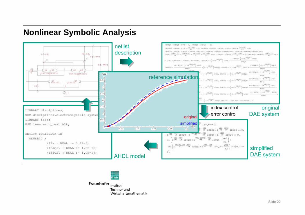
Nonlinear Symbolic Analysis
AHDL model
netlistdescription
originalDAE system
simplifiedDAE system
index controlerror control
reference simulation
originalsimplified
Slide 23
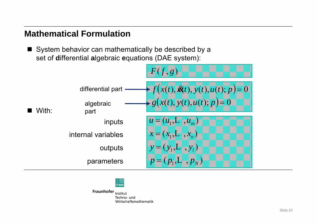
Mathematical Formulation
System behavior can mathematically be described by aset of differential algebraic equations (DAE system):
( )( ) 0);(),(),(
0);(),(),(),(=
=ptutytxg
ptutytxtxf &
),( gfF
differential part
algebraic part
1
1
1
1
( , , )( , , )( , , )( , , )
m
n
l
N
u u ux x xy y yp p p
==
=
=
LLLL
With:inputs
internal variables
outputs
parameters
Slide 24
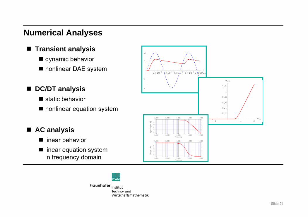
Numerical Analyses
Transient analysisdynamic behaviornonlinear DAE system
DC/DT analysisstatic behaviornonlinear equation system
AC analysislinear behaviorlinear equation systemin frequency domain
2×10 6 4×10 6 6×10 6 8×10 6 0.00001t
2
1
1
2
2 1 1 2Vin
0.2
0.4
0.6
0.8
1
1.2
vout
1.0E0 1.0E2 1.0E4 1.0E6 1.0E8Frequency
50
40
30
20
10
0
ed
ut
in
ga
M�Bd� 1.0E0 1.0E2 1.0E4 1.0E6 1.0E8
1.0E0 1.0E2 1.0E4 1.0E6 1.0E8Frequency
80
60
40
20
0
es
ah
P�ged�
1.0E0 1.0E2 1.0E4 1.0E6 1.0E8
Slide 25
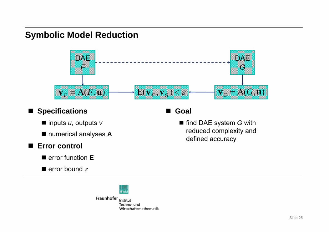
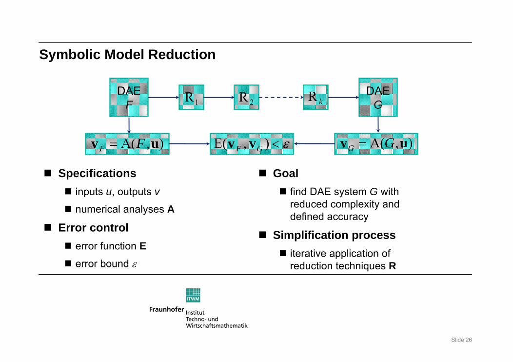
Symbolic Model Reduction
Specificationsinputs u, outputs v
numerical analyses A
Error controlerror function Eerror bound ε
),A( uv FF =
DAEF
DAEG
),A( uv GG =ε<),E( GF vv
Goalfind DAE system G with reduced complexity and defined accuracy
Slide 26
Symbolic Model Reduction
),A( uv FF =
DAEF
DAEG
),A( uv GG =ε<),E( GF vv
1R kR2R
Specificationsinputs u, outputs v
numerical analyses A
Error controlerror function Eerror bound ε
Goalfind DAE system G with reduced complexity and defined accuracy
Simplification processiterative application of reduction techniques R
Slide 27
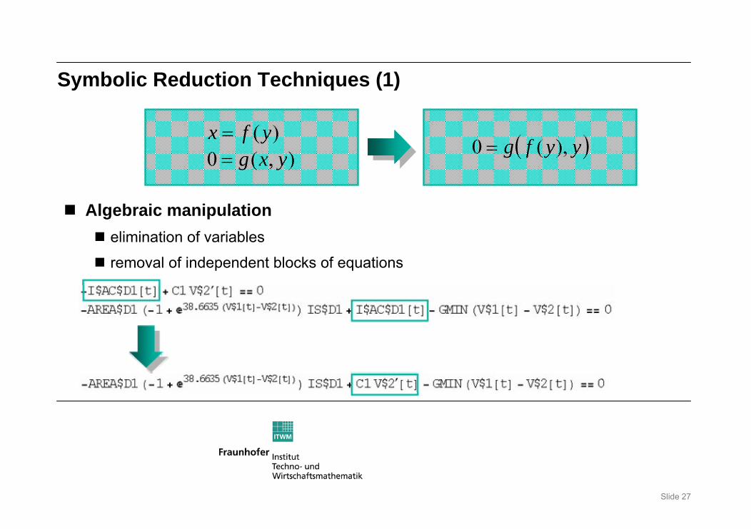
Symbolic Reduction Techniques (1)
Algebraic manipulationelimination of variables
removal of independent blocks of equations
),(0)(yxg
yfx== ( )yyfg ),(0 =
Slide 28
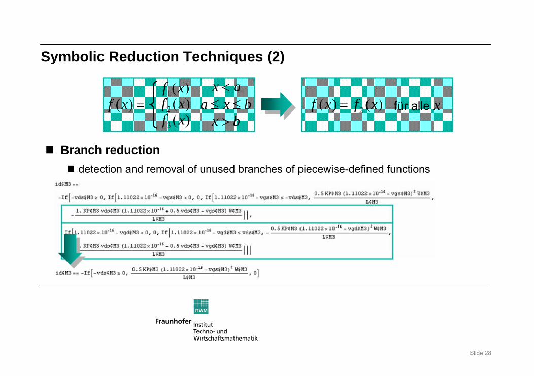
Symbolic Reduction Techniques (2)
Branch reductiondetection and removal of unused branches of piecewise-defined functions
=)(xf)(1 xf ax <)(2 xf bxa ≤≤)(3 xf bx >
)()( 2 xfxf = für alle x
Slide 29
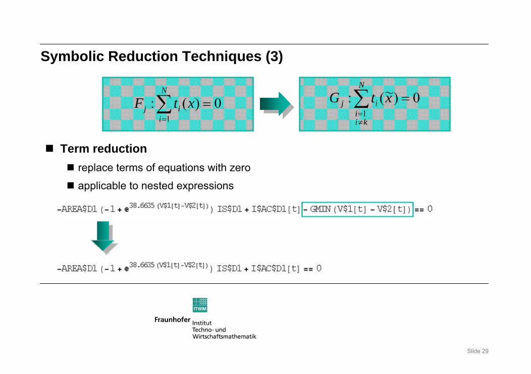
Symbolic Reduction Techniques (3)
0)(:1
=∑=
N
iij xtF 0)~(:
1=∑
≠=
N
kii
ij xtG
Term reductionreplace terms of equations with zero
applicable to nested expressions
Slide 30
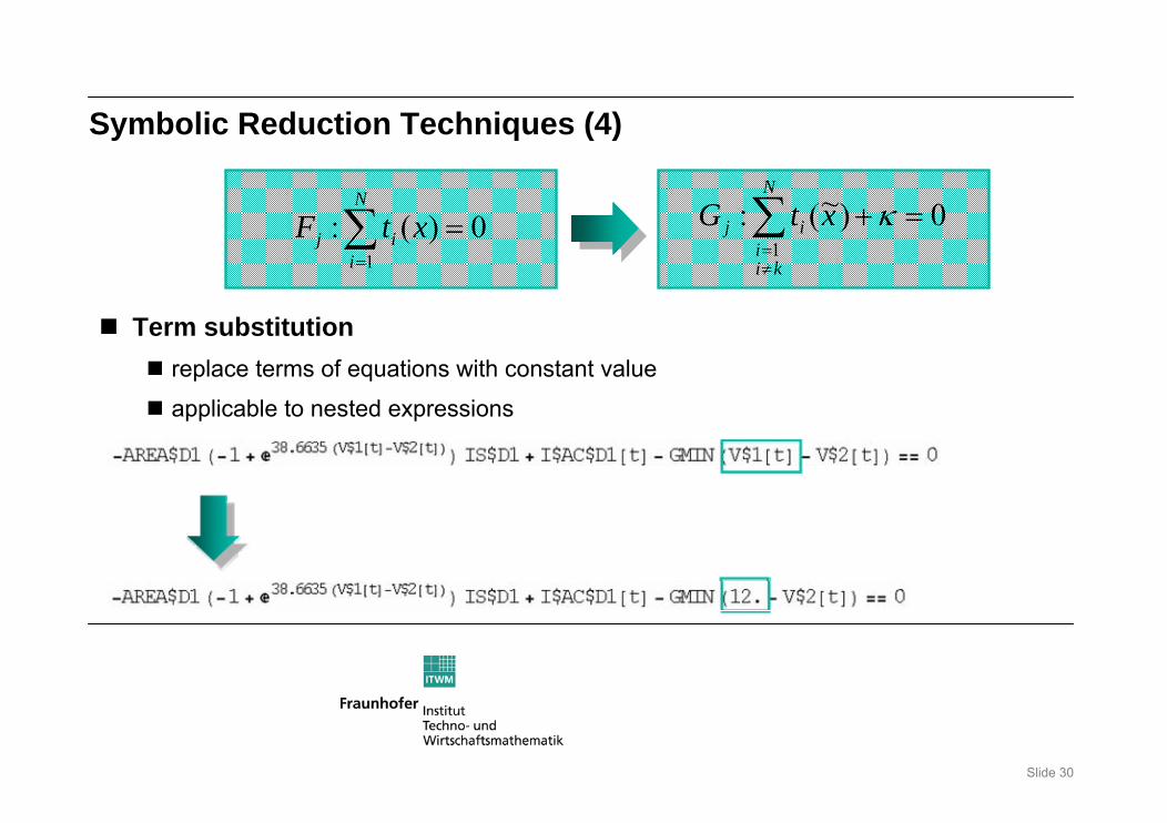
Symbolic Reduction Techniques (4)
0)(:1
=∑=
N
iij xtF 0)~(:
1=+∑
≠=
κN
kii
ij xtG
Term substitutionreplace terms of equations with constant value
applicable to nested expressions
Slide 31
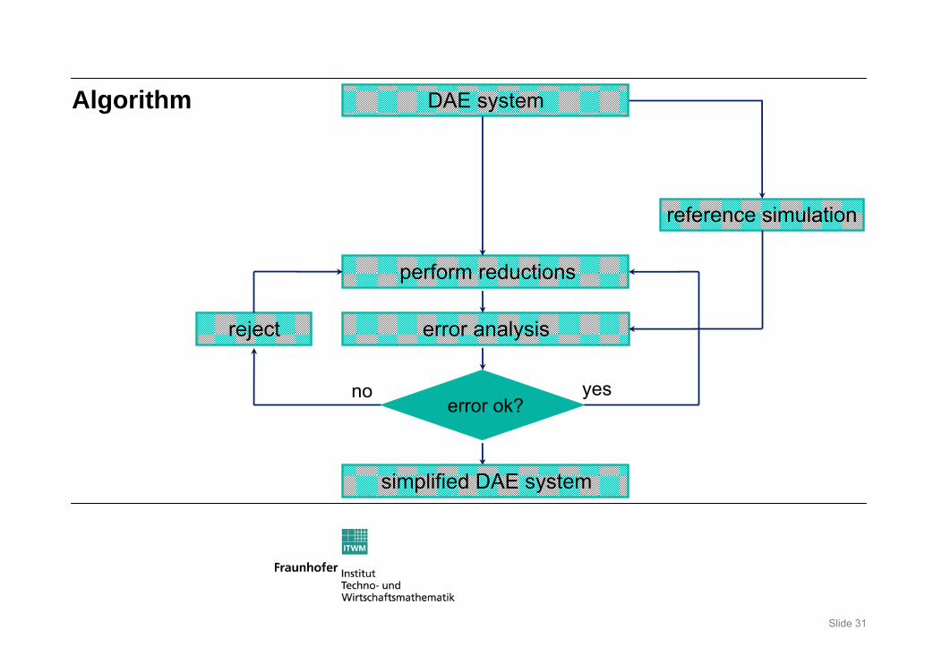
Algorithm
perform reductions
error ok?yes
reference simulation
DAE system
simplified DAE system
reject error analysis
no
Slide 32
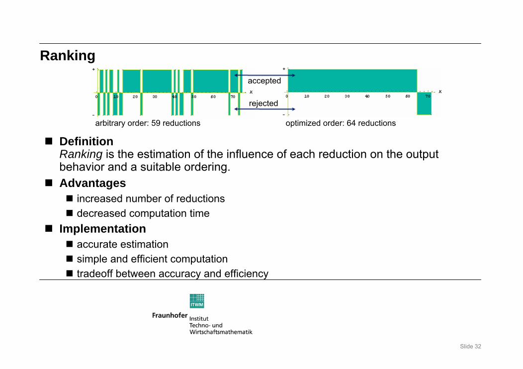
Ranking
arbitrary order: 59 reductions optimized order: 64 reductions
DefinitionRanking is the estimation of the influence of each reduction on the output behavior and a suitable ordering.Advantages
increased number of reductionsdecreased computation time
Implementationaccurate estimationsimple and efficient computationtradeoff between accuracy and efficiency
rejected
accepted
Slide 33
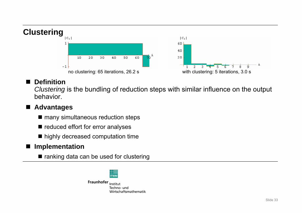
Clustering
no clustering: 65 iterations, 26.2 s with clustering: 5 iterations, 3.0 s
DefinitionClustering is the bundling of reduction steps with similar influence on the output behavior. Advantages
many simultaneous reduction stepsreduced effort for error analyseshighly decreased computation time
Implementationranking data can be used for clustering
Slide 34
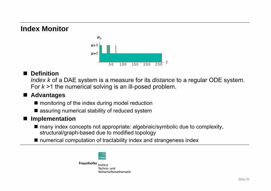
Index Monitor
DefinitionIndex k of a DAE system is a measure for its distance to a regular ODE system.For k >1 the numerical solving is an ill-posed problem.Advantages
monitoring of the index during model reductionassuring numerical stability of reduced system
Implementationmany index concepts not appropriate: algebraic/symbolic due to complexity, structural/graph-based due to modified topologynumerical computation of tractability index and strangeness index
Slide 35
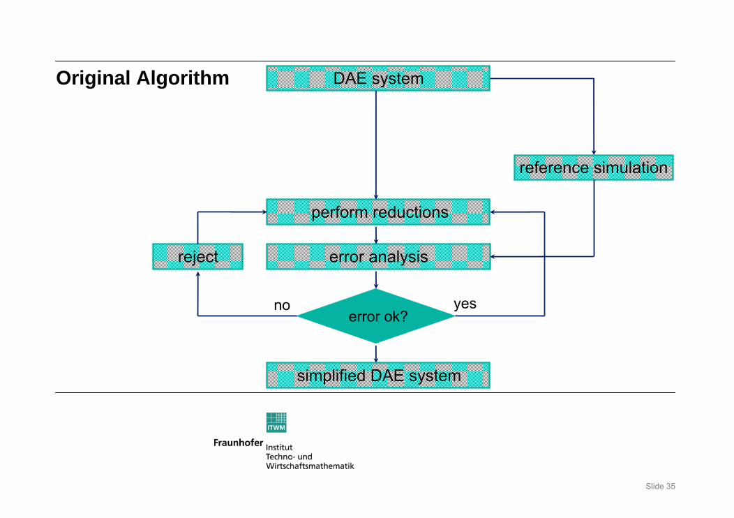
Original Algorithm
perform reductions
error ok?yes
reference simulation
DAE system
simplified DAE system
reject error analysis
no
Slide 36
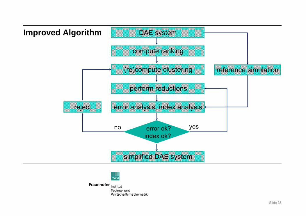
Improved Algorithm
perform reductions
yes
reference simulation
DAE system
simplified DAE system
reject error analysis, index analysis
no
(re)compute clustering
compute ranking
error ok?index ok?
Slide 37
Example Application: Operational Amplifier
VB
Vsig
1k
RF1
I4
VCC
VDD
I1
I3
Q2N2907AQ4
Q2N2222
Q5
Q2N2907A
Q3
Q2N2907A
Q7 Q8Q2N2907A
Q2
Q2N2222
Q1
Q2N2222
Q6
Q2N2907A
R1 20
R2 20
10k
RF2
RL 100k
Comp
30p
0
0
0
0
0
VDB
8
10
7
3
in
413
11
6
2
2
12
1
5
9
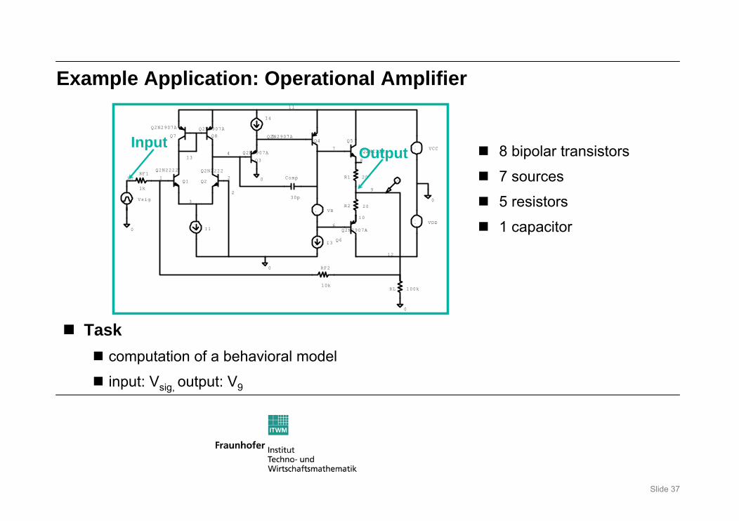
InputOutput 8 bipolar transistors
7 sources
5 resistors
1 capacitor
Taskcomputation of a behavioral model
input: Vsig, output: V9
Slide 38
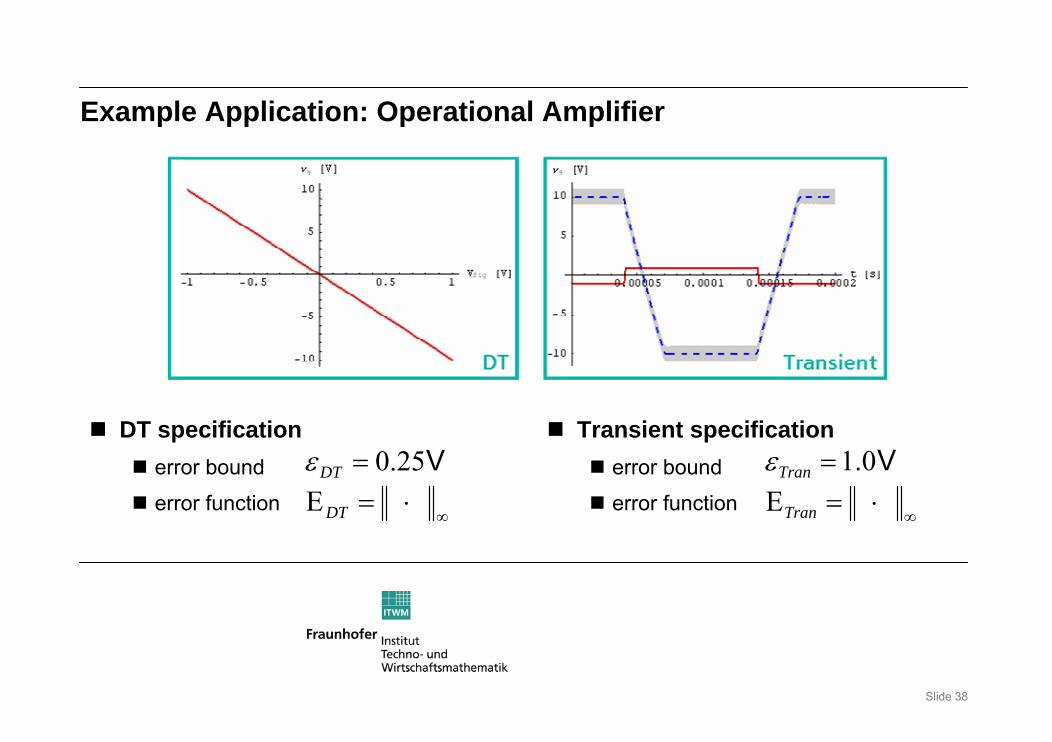
Example Application: Operational Amplifier
DT specificationerror bound
error function
Transient specificationerror bound
error function∞
⋅==
DT
DT
E25.0 Vε
∞⋅=
=
Tran
Tran
E0.1 Vε
Slide 39
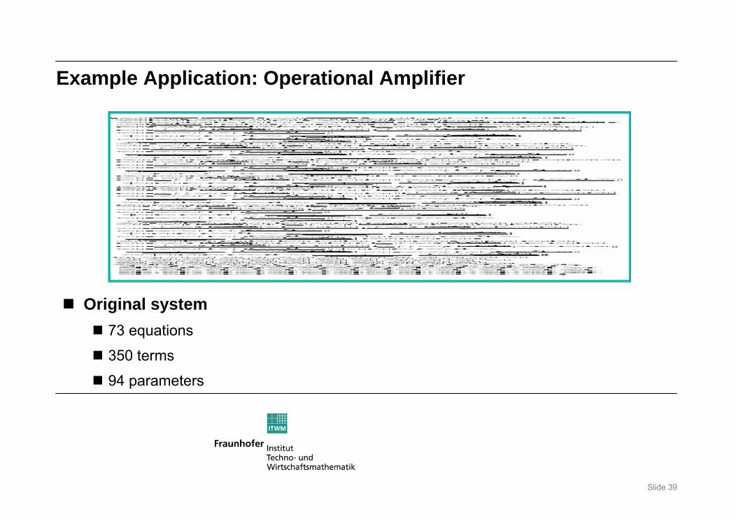
Example Application: Operational Amplifier
Original system73 equations
350 terms
94 parameters
Slide 40
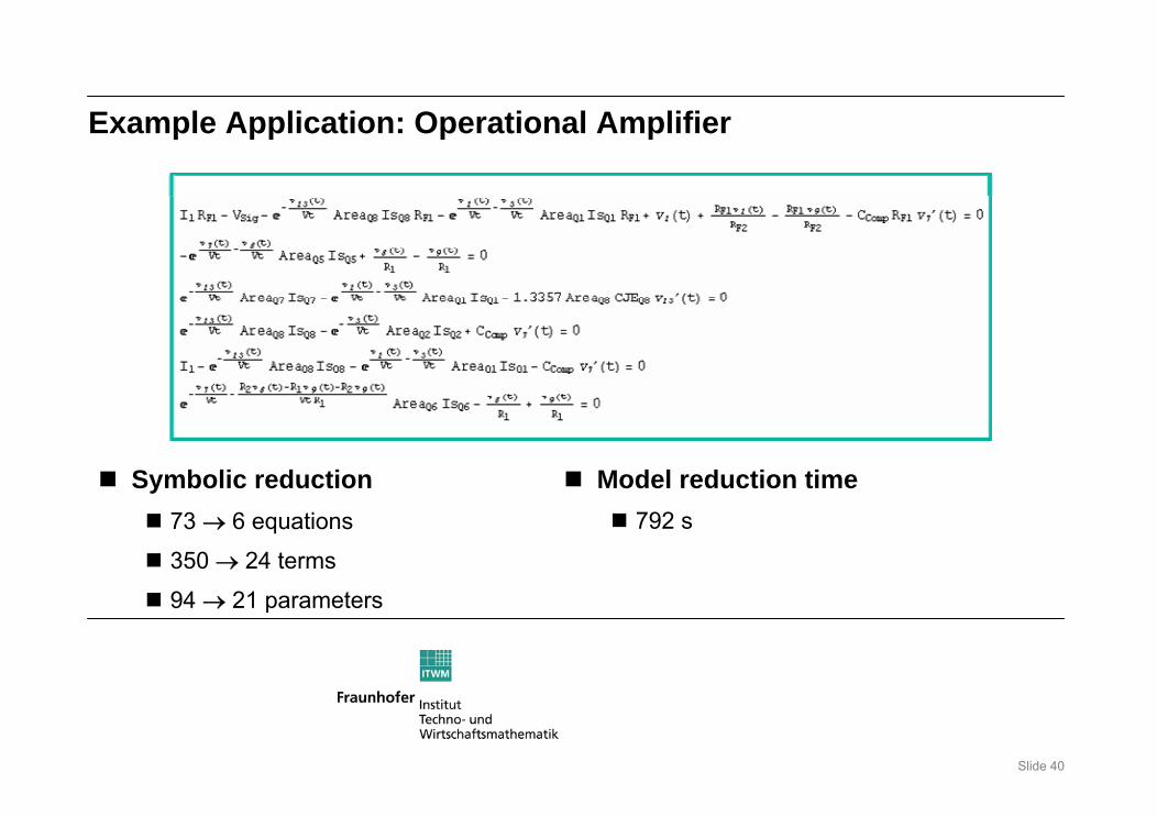
Example Application: Operational Amplifier
Symbolic reduction73 → 6 equations
350 → 24 terms
94 → 21 parameters
Model reduction time792 s
Slide 41
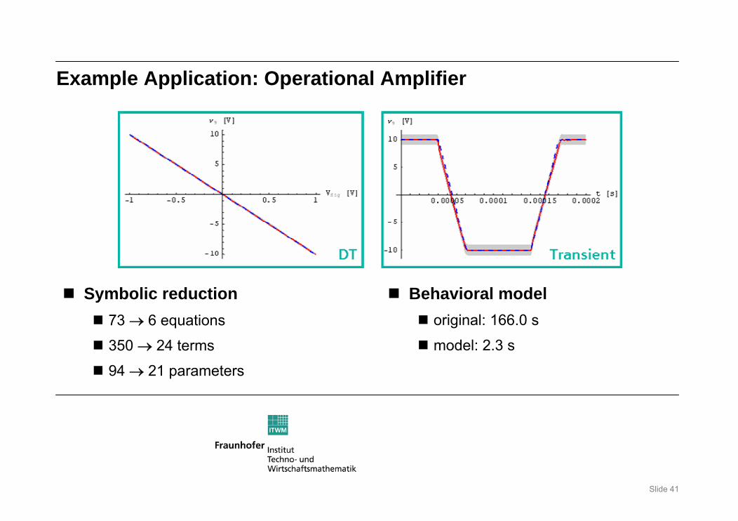
Example Application: Operational Amplifier
Symbolic reduction73 → 6 equations
350 → 24 terms
94 → 21 parameters
Behavioral modeloriginal: 166.0 s
model: 2.3 s
Slide 42
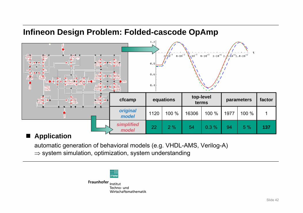
Infineon Design Problem: Folded-cascode OpAmp
cfcamp equations top-levelterms parameters factor
originalmodel 1120 100 % 16306 100 % 1977 100 % 1
simplified model 22 2 % 54 0.3 % 94 5 % 137
Applicationautomatic generation of behavioral models (e.g. VHDL-AMS, Verilog-A)⇒ system simulation, optimization, system understanding
Slide 43
Nonlinear Symbolic Analysis: Benefits and Limits
• support for automated generation of behavioralmodels for different behavioral modeling languagesand simulators
• automatic and error-controlled complexity reduction • supported analysis modes: DC-Transfer, AC, Transient
Benefits
Limits • limited circuit size (currently up to 20 transistors)• algorithms under development• explicit symbolic results for static systems
in general not possible
• due to the general mathematical conceptthe methods are also applicable to other domains(e.g. system simulation of mechatronical systems)
Synergies
Slide 44
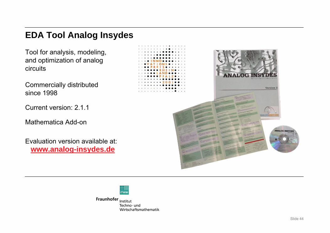
Tool for analysis, modeling,and optimization of analogcircuits
Commercially distributedsince 1998
Current version: 2.1.1
Mathematica Add-on
Evaluation version available at:www.analog-insydes.de
EDA Tool Analog Insydes
Slide 45
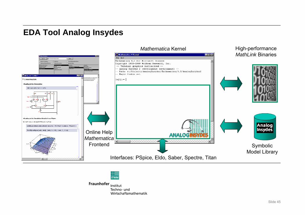
EDA Tool Analog Insydes
Mathematica Kernel
Interfaces: PSpice, Eldo, Saber, Spectre, Titan
High-performanceMathLink Binaries
SymbolicModel Library
Online HelpMathematica
Frontend
Slide 46
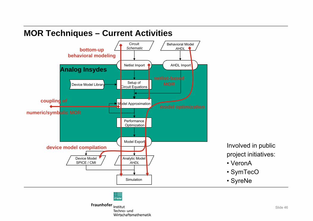
MOR Techniques – Current Activities
bottom-upbehavioral modeling
model optimization
device model compilation
Analog Insydes
CircuitSchematic
Setup ofCircuit Equations
Model Approximation
Analytic ModelAHDL
Netlist Import
Device Model Library
PerformanceOptimization
Device ModelSPICE / CMI
Model Export
AHDL Import
Behavioral ModelAHDL
Simulation
coupling of
numeric/symbolic MOR
Involved in publicproject initiatives: • VeronA• SymTecO• SyreNe
netlist-basedMOR
Slide 47
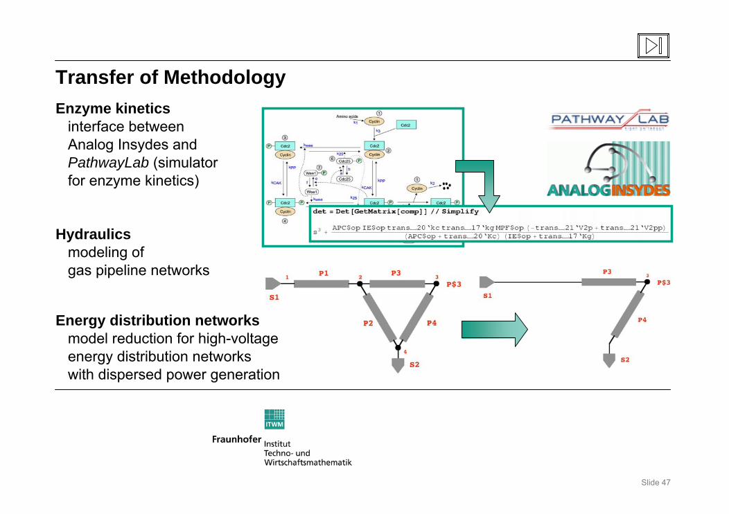
Transfer of Methodology
Hydraulicsmodeling ofgas pipeline networks
Enzyme kineticsinterface between Analog Insydes andPathwayLab (simulatorfor enzyme kinetics)
Energy distribution networksmodel reduction for high-voltageenergy distribution networkswith dispersed power generation
Slide 48
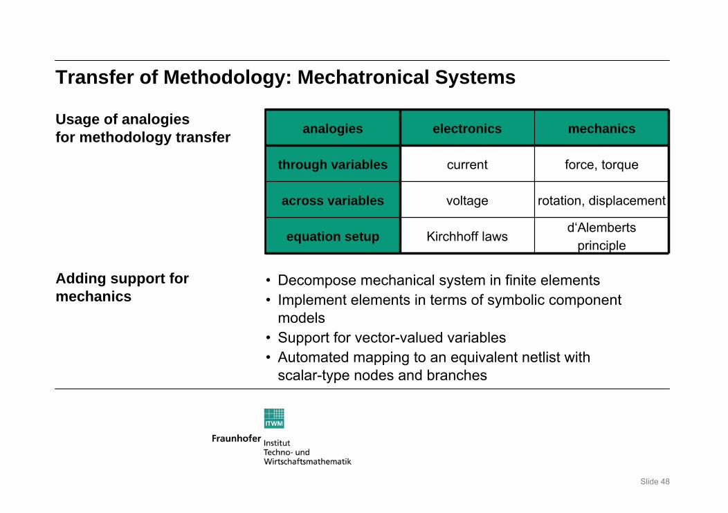
Transfer of Methodology: Mechatronical Systems
analogies electronics mechanics
through variables current force, torque
across variables voltage rotation, displacement
equation setup Kirchhoff lawsd‘Alemberts
principle
Usage of analogiesfor methodology transfer
• Decompose mechanical system in finite elements• Implement elements in terms of symbolic component
models• Support for vector-valued variables• Automated mapping to an equivalent netlist with
scalar-type nodes and branches
Adding support formechanics
Slide 49
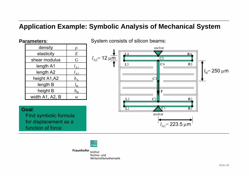
Application Example: Symbolic Analysis of Mechanical System
density ρelasticity E
shear modulus Glength A1 lA1
length A2 lA2
height A1,A2 hA
length B lBheight B hB
width A1, A2, B w
Parameters: System consists of silicon beams:
lA1= 223.5 μm
lA2= 12 μm
lB= 250 μm
Goal:Find symbolic formulafor displacement as afunction of force
Slide 50
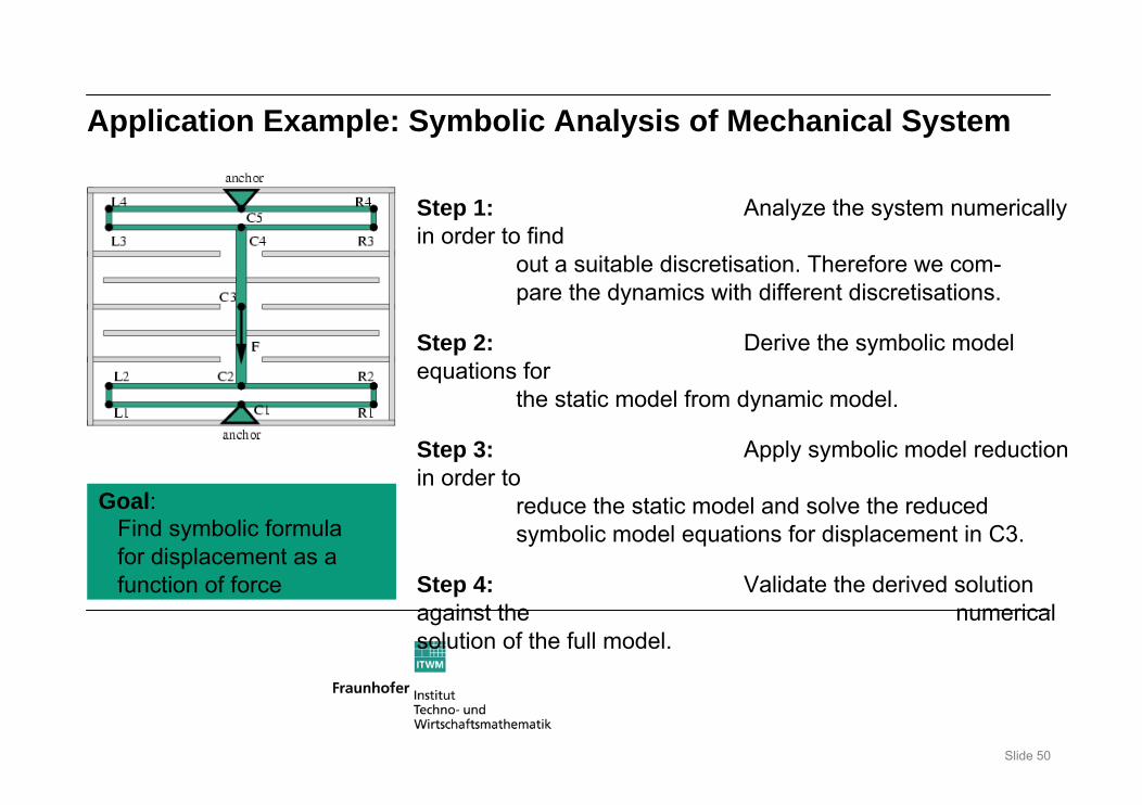
Application Example: Symbolic Analysis of Mechanical System
Goal:Find symbolic formulafor displacement as afunction of force
Step 1: Analyze the system numerically in order to find
out a suitable discretisation. Therefore we com-pare the dynamics with different discretisations.
Step 2: Derive the symbolic model equations for
the static model from dynamic model.
Step 3: Apply symbolic model reduction in order to
reduce the static model and solve the reduced symbolic model equations for displacement in C3.
Step 4: Validate the derived solution against the numerical solution of the full model.
Slide 51
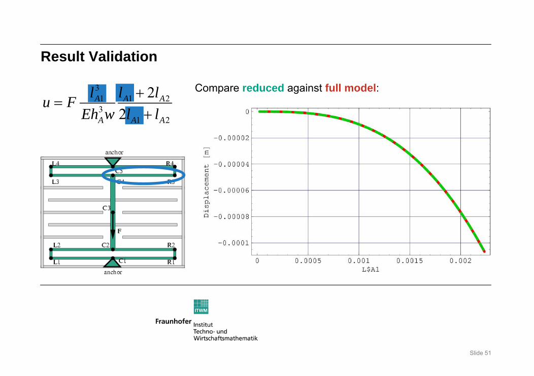
31 1 23
1 2
22
A A A
A A A
l l lu FEh w l l
+=
+
Result Validation
Compare reduced against full model:
Slide 52
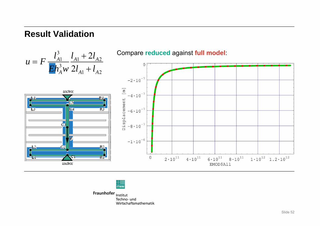
Result Validation
31 1 23
1 2
22
A A A
A A A
l l lu FEh w l l
+=
+
Compare reduced against full model:
Slide 53
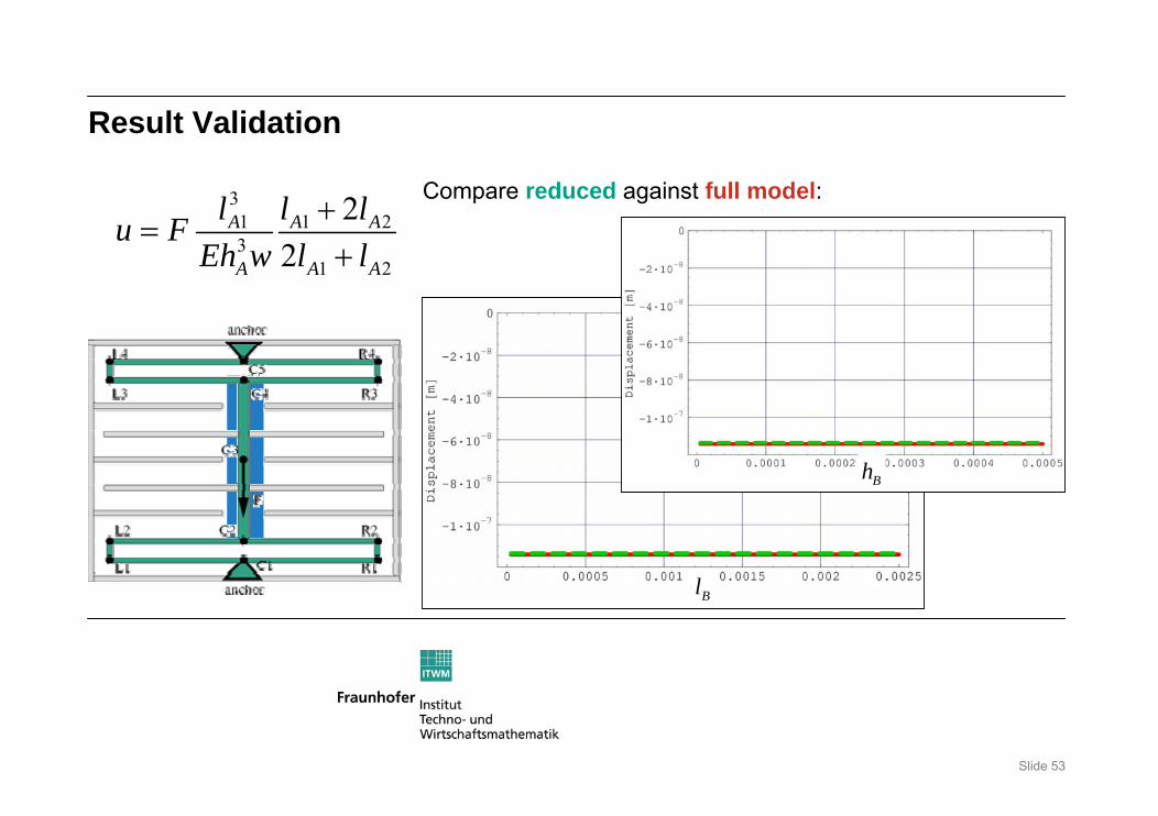
Result Validation
31 1 23
1 2
22
A A A
A A A
l l lu FEh w l l
+=
+
Bh
Bl
Compare reduced against full model:
Slide 54
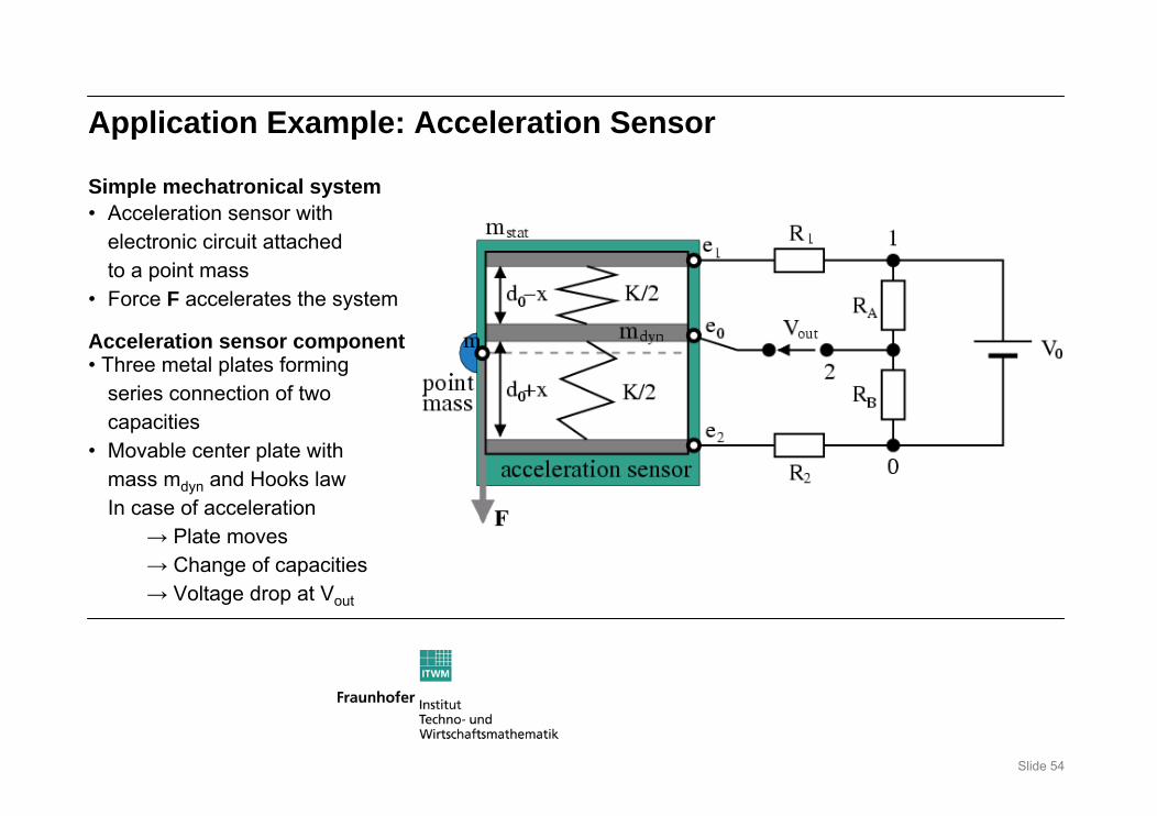
Application Example: Acceleration Sensor
• Three metal plates formingseries connection of twocapacities
• Movable center plate withmass mdyn and Hooks lawIn case of acceleration
→ Plate moves→ Change of capacities→ Voltage drop at Vout
Simple mechatronical system• Acceleration sensor with
electronic circuit attachedto a point mass
• Force F accelerates the system
Acceleration sensor component
Slide 55
Application Example: Model Reduction
Analog Insydes command CancelTerms approximates the DAE system:
Slide 56
Application Example: Model Reduction
Analog Insydes command CancelTerms approximates the DAE system
Slide 57
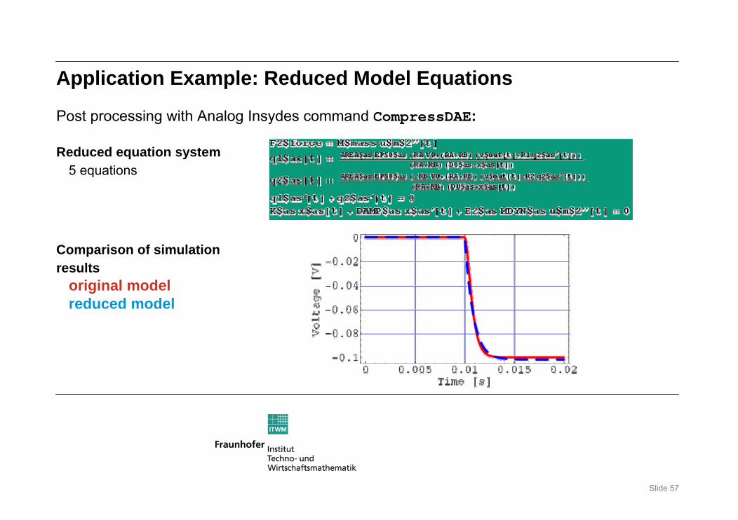
Application Example: Reduced Model Equations
Post processing with Analog Insydes command CompressDAE:
Reduced equation system5 equations
Comparison of simulationresults
original modelreduced model
Slide 58
Summary and Outlook
• Application of symbolic analysis only possible usingapproximation techniques coupled with numericsimulation
• Linear symbolic analysis used successfully for industrialcircuit analysis tasks
• Nonlinear symbolic analysis under development withpromising results
Summary
Outlook • Extension of nonlinear simplification methods
• Extension towards support for multi-physics systems
• Integration of symbolic analysis into industrial designflows