Embed Size (px)
Citation preview

SCRS/2015/167 Collect. Vol. Sci. Pap. ICCAT, 72(7): 1667-1693 (2016)
1667
AN ILLUSTRATIVE EXAMPLE OF A MANAGEMENT PROCEDURE FOR
EASTERN NORTH ATLANTIC BLUEFIN TUNA
R A Rademeyer1 and D S Butterworth1
SUMMARY
This document provides an illustrative example of the development of Candidate Management
Procedures (MPs) for the Eastern North Atlantic bluefin tuna resource. Its purpose is to draw
attention to key components of this process, including the specification of a number of
alternative Operating Models (OMs) which describe plausible dynamics for the resource, the
choices of abundance indices for use for input to MPs and of the error structures associated
with the generation of future data corresponding to those indices, and consideration of key
performance statistics related to future catch levels and resource conservation to allow
consideration of the different trade-offs between these for alternative MPs. The MPs examined
use a combination of target and slope based approaches applied to simulated future abundance
indices from Japanese longline operations and a larval survey in an area of the western
Mediterranean. MP trials are carried out for four OMs which reflect alternative resource
assessments and choices for relationships between recruitment and spawning biomass. The
greatest challenge appears to come from a scenario with both high and low recruitment
regimes when there is a change from the former to the latter. If catches are allowed to go high
to benefit from the period of high recruitment, can the change in regime be identified
sufficiently soon to allow for adequate catch limit reductions to ensure resource conservation
during the later years of lower recruitments?
RÉSUMÉ
Ce document fournit un exemple illustrant le développement de procédures de gestion possibles
(MP) pour la ressource de thon rouge de l'Atlantique Nord-Est. Son but est d'attirer l'attention
sur des éléments clés de ce processus, y compris la spécification d'un nombre de modèles
opérationnels alternatifs (OM) qui décrivent la dynamique plausible pour la ressource, les
choix des indices d'abondance à utiliser pour la saisie dans les procédures de gestion et des
structures d'erreur associées à la création de données futures correspondant à ces indices, et
l'examen de statistiques de performance clés associées à de futurs niveaux de capture et à la
conservation de la ressource pour permettre d'examiner les différents avantages et
inconvénients entre ceux-ci pour obtenir des procédures de gestion alternatives. Les procédures
de gestion examinées utilisent une combinaison d'approches basées sur la cible et sur la pente
appliquées à de futurs indices d’abondance simulés à partir des opérations palangrières
japonaises et d'une prospection larvaire dans une zone de la Méditerranée occidentale. Les
essais de procédures de gestion sont effectués pour quatre modèles opérationnels qui reflètent
des évaluations des ressources alternatives et des choix pour les relations entre le recrutement
et la biomasse reproductrice. Le plus grand défi semble provenir d'un scénario présentant des
régimes de recrutement à la fois fort et faible lorsqu'il y a un changement du premier au
dernier. Si on permet que les prises augmentent afin de bénéficier de la période de fort
recrutement, est-ce que le changement de régime peut être identifié suffisamment à l'avance
pour permettre des réductions des limites de capture adéquates pour garantir la conservation
des ressources au cours des années ultérieures de recrutement plus faible ?
1Marine Resource Assessment and Management Group, University of Cape Town, South Africa, [email protected]

1668
RESUMEN
Este documento presenta un ejemplo ilustrativo del desarrollo de posibles procedimientos de
ordenación (MP) para el atún rojo del Atlántico norte oriental. Su propósito es llamar la
atención sobre los componentes clave de este proceso, incluida la especificación de un número
de modelos operativos (OM) alternativos que describen una dinámica plausible para este
recurso, la elección de índices de abundancia para utilizarlos como entrada en los MP y de
estructuras de error asociadas con la generación de datos futuros correspondientes a estos
índices, así como la consideración de estadísticas clave de rendimiento relacionadas con
niveles futuros de captura y con la conservación del recurso para permitir la consideración de
las distintas ventajas e inconvenientes entre ellas para MP alternativos. Los MP examinados
utilizan una combinación de enfoques basados en el objetivo y en la pendiente aplicados a
índices de abundancia futuros simulados procedentes de las operaciones de palangre japonés y
a una prospección de larvas en una zona del Mediterráneo occidental. Los ensayos de los MP
se han llevado a cabo para cuatro OM, que reflejan evaluaciones alternativas del recurso y
elecciones para la relación entre reclutamiento y biomasa reproductora. El mayor desafío
parece proceder de un escenario con ambos regímenes de reclutamiento, alto y bajo, cuando
hay un cambio del primero al segundo. Si se permite aumentar las capturas para beneficiarse
del periodo de alto reclutamiento, ¿podría el cambio de régimen identificarse lo
suficientemente pronto para permitir reducciones adecuadas en el límite de captura con miras
a garantizar la conservación del recurso durante los últimos años de reclutamientos más
bajos?
KEYWORDS
Management procedure, Bluefin tuna, eastern North Atlantic, recruitment, regime shift
1 Introduction
The Management Strategy Evaluation (MSE)/Management Procedure (MP) process is subtle and sometimes
complex, and therefore it can be difficult to grasp the essences and implications if presented only in an abstract
way. In an attempt to aid the process for enhanced understanding, this document provides an illustrative example
of the development of Candidate Management Procedures (MPs) for the Eastern North Atlantic bluefin tuna
resource. Its purpose is to draw attention to key components of this process, especially the catch vs resource
depletion risk considerations that arise, so as to guide the further development of the MSE/MP process for
bluefin tuna within ICCAT.
The document first develops Operating Models (OMs) to be used to test candidate MPs (CMPs) which are based
on statistical catch-at-length (SCAL) assessments of the resource using the most recent data available, and also
sets out a few options for projecting these dynamics into the future in line with plausible future recruitment
scenarios. The data series to be used as input to the CMPs are specified, and the process used to generate future
associated observed values for these developed. Some relatively simple empirical CMPs are specified, and these
are applied to the four OMs specified for the resource to determine catch vs resource depletion risk performance.
Finally the implications of the outcomes from these calculations for the further development of the ICCAT
MSE/MP process for bluefin tuna are discussed.
2 Data and Methods
2.1 Data
The testing of the illustrative MPs in this paper requires the availability of a set of OMs, which in turn are
conditioned on the data available by developing them as SCAL assessments of the resource. The data used for
input to those assessments are listed in Appendix A, and are as originally provided in Bonhommeau et al.
(2014). Note that the assessment runs from 1950 to 2013.

1669
2.2 SCAL assessments
Appendix B provides details of the SCAL methodology applied, together with specifications for the Reference
Case (RC) OM. Figure 1 shows the spawning biomass and recruitment time series estimated for the RC, and is
followed by some further results and diagnostics: Figure 2 shows the stock-recruitment (SR) relationship and
corresponding residuals, Figure 3 shows the fits to the relative abundance index series for RC, and Figure 4
plots the commercial selectivities and the fits to CAL data.
It is immediately evident from Figure 2 that although the assessment model does respond to the recent increases
in the JLL_NEA and larval indices, the estimated abundance fails to increase to as large an extent as these
indices. To develop an alternative OM (scenario S1) that fits these indices better, the assessment was repeated
giving more weight (x12) for index data from 2010 onwards for the JLL_NEA and larval index series.
2.3 Projections
The projection methodology used is detailed in Appendix C. Note that although the assessment extends only to
2013, the 2014 catch is taken as equal to the 2014 TAC and the Commission has sets catch limits for 2015 to
2017 (details in Appendix C).
However the time series of recruitments estimated for the RC are suggestive of a shift from a lower to a higher
productivity in 1983 (see Figure 5). Scenario S2 thus supposes a regime shift that year, so that periods before
and after that date reflect different average recruitments and hence also different average pristine (unexploited)
abundances. In 2013 the higher recruitment scenario applies, but there is no guarantee that that will continue
through all future years. Hence two further OMs are defined: in the first (S2a) the high recruitment does continue
throughout the projection period, whereas in the second (S2b) the resource reverts to the lower recruitment
regime from 2020 onwards.
Figure 6 shows the historical spawning biomass trajectories for the RC, S1 and S2 (note that the S2a and S2b
scenarios are not distinguished here as they diverge only in the future).
Candidate Management Procedures
In the interests of simplicity for this illustrative exercise, the MPs investigated have been restricted to two
indices of abundance, the JPLL_NEA and the larval indices. These were selected, in part, because both seem
likely to continue and because both reflect the large recent upward change in the abundance of the resource.
Further these MPs are empirical, computing TACs directly from the abundance indices. There are two common
and simple approaches to developing such empirical MPs: target based (the TAC is adjusted up or down
depending on whether the index is above or below a chosen target level) and slope-based where this adjustment
is up or down as the recent trend in the index is either positive or negative. Usually the former approach is
preferred as it provides more stable outputs, but that alone is not appropriate here given the two regime nature of
the resource (e.g. an appropriate target under the higher recruitment scenario would be unachievable for the
lower recruitment scenario and hence lead to TACs reducing to zero). Thus a combination of the two approaches
has been attempted. The first of these takes the following form.
CMP1_x:
11
targ
//1J
JsTACTAC
y
downupydownupyy (1)
where
ys is the average of trend estimates for each of the two indices, where this trend estimate is provided by the
slope of a log-linear regression of the index against year over the last ten years (y-10 to y-1);
ii
i
i
yy
J
J
J
J1
targtarg
where i
yJ is the average of the values of index i over the most recent five years (y-5 to y-1); and
1670
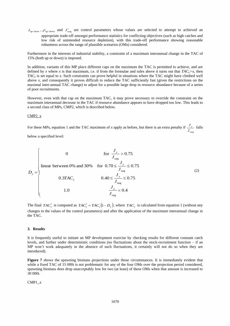
downup / ,downup / and iJ targ
are control parameters whose values are selected to attempt to achieved an
appropriate trade-off amongst performance statistics for conflicting objectives (such as high catches and
low risk of unintended resource depletion), with this trade-off performance showing reasonable
robustness across the range of plausible scenarios (OMs) considered.
Furthermore in the interests of industrial stability, a constraint of a maximum interannual change in the TAC of
15% (both up or down) is imposed.
In addition, variants of this MP place different caps on the maximum the TAC is permitted to achieve, and are
defined by x where x is that maximum, i.e. if from the formulae and rules above it turns out that TACy>x, then
TACy is set equal to x. Such constraints can prove helpful in situations where the TAC might have climbed well
above x, and consequently it proves difficult to reduce the TAC sufficiently fast (given the restrictions on the
maximal inter-annual TAC change) to adjust for a possible large drop in resource abundance because of a series
of poor recruitments.
However, even with that cap on the maximum TAC, it may prove necessary to override the constraint on the
maximum interannual decrease in the TAC if resource abundance appears to have dropped too low. This leads to
a second class of MPs, CMP2, which is described below.
CMP2_x
For these MPs, equation 1 and the TAC maximum of x apply as before, but there is an extra penalty if targJ
J y falls
below a specified level:
4.00.1
75.00.403.0
75.00.70for %30 and %0between linear
75.0for 0
targ
targ
targ
targ
J
J
J
JTAC
J
J
J
J
D
y
y
y
y
y
y
(2)
The final *
yTAC is computed as yyy DTACTAC 1* , where yTAC is calculated from equation 1 (without any
changes to the values of the control parameters) and after the application of the maximum interannual change in
the TAC.
3. Results
It is frequently useful to initiate an MP development exercise by checking results for different constant catch
levels, and further under deterministic conditions (no fluctuations about the stock-recruitment function – if an
MP won’t work adequately in the absence of such fluctuations, it certainly will not do so when they are
introduced).
Figure 7 shows the spawning biomass projections under those circumstances. It is immediately evident that
while a fixed TAC of 15 000t is not problematic for any of the four OMs over the projection period considered,
spawning biomass does drop unacceptably low for two (at least) of these OMs when that amount is increased to
30 000t.
CMP1_x

1671
The following control parameters were selected for CMP 1:
Control parameter Value
up 0.03
down 0.15
up 0.03
down 0.15
Jtarg - JPLL_NEA 0.95
Jtarg – larval 1.70
where the values of Jtarg are about 50% of the average of the levels to be expected for S2a and S2b in the absence
of exploitation.
Results have been explored for values of x = no_cap, 40 000 and 30 000t. Figure 8 shows the results for the
40 000t cap particularly for catch and spawning biomass and their probability intervals for all four OMs, with
some no_cap results are shown to provide a contrast. Figure 9 repeats this for the 30 000t cap, and Figure 10
contrasts results for the three variants of CMP1 for the lower 2.5%iles for spawning biomass, and the median
and upper 2.5%iles for catch.
Figure 11 contrasts CMP1 and CMP2 behaviour for spawning biomass and catch trajectories for all four OMs
(i.e. to check whether more stringent rules for catch reductions when the combined abundance index J drops to
low levels are successful at avoiding instances of very low abundances, particularly for the fourth OM where
there is a switch from the higher to the lower recruitment regime. Figure 11 is for the case of a 40 000t cap on
the TAC; Figure 12 repeats those results for a 30 000t cap.
4. Discussion
Figure 8 reflects satisfactory performance for the RC and the higher recruitment regime scenario S2a under
CMP1. However TACs rise too high for scenario S1 (which reflects a better fit to recent JLL_NEA and larval
abundance indices) and S2b (the switch to the lower recruitment regime), and these lead to subsequent
undesirable levels of decline in spawning biomass. This decline is ameliorated somewhat for scenario S1 given
the 40 000t TAC cap, but it needs this cap to be lowered to 30 000t to see some small improvement in this regard
for scenario S2b (Figure 9). However, such amelioration comes at a cost, particularly in terms of catch under
scenario S2a, as is evident from the comparisons across the three choices for the level of this TAC cap in Figure
10.
Given the extra restrictions of CMP2 plus the 30 000t TAC cap, there is some further improvement as regards
resource depletion for scenario S2b, but this comes at the further expense of greater (sometimes substantial)
TAC declines after 2030 (see Figure 12).
More sophisticated algorithms might attain better performance still than evident in Figures 11 and 12, but their
development is not really an immediate priority, given the illustrative nature intended for this document. The
problem arises because highly noisy (CV > 70%) indices of abundance provide indications of stock decline that
are too imprecise and too delayed to give a clear indication of the immediate status of the resource. Certainly a
more refined further attempt at an MP might include further information inputs to offset this.
However this does serve to draw attention to some key considerations in the MP development process for North
Atlantic bluefin tuna:
a) careful consideration is needed as to what monitoring data (particularly abundance indices) will almost
certainly be available in the future, so that any candidate MPs can be designed around those;
b) equally, as careful consideration is needed regarding specification of the error structures associated with
such information (specifically biases and variances) for projection purposes for the MP testing process
– hopefully such may lead to defensibly better precision than the >70% CVs applied in these illustrative
analyses; and

1672
c) thorough discussion is needed to specify future realistic recruitment scenarios and to accord then some
form of relative plausibility weights for the eventual process of selecting an MP that gives an acceptable
catch vs depletion risk trade-off.
Reference
Bonhommeau S., Kimoto, A., Fromentin, J.M., Kell, L., Arrizabalaga, H., Walter, J.F., Ortiz de Urbina, J.,
Zarrad, R., Kitakado, T., Takeuchi, Y., Ortiz, M. and Palma, C. 2014. Update of the Eastern and
Mediterranean Atlantic bluefin tuna stock. ICCAT Col. Vol. Sci. Pap. 71(3): 1366-1382.

1673
Figure 1. Spawning biomass and recruitment (number of 1-year-olds, N1) trajectories for Eastern North Atlantic
bluefin tuna for the SCAL Reference Case.
Figure 2. Stock-recruitment relationships (left-hand column) and time series of stock-recruitment residuals for
the SCAL Reference Case. Spawning stock biomass (Bsp) is in mt. The replacement line is also shown; this
intercepts the stock-recruitment plot where Bsp = Ksp.
1674
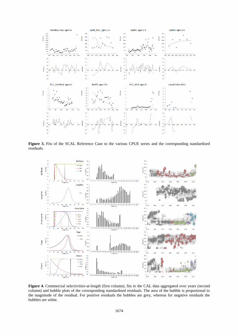
Figure 3. Fits of the SCAL Reference Case to the various CPUE series and the corresponding standardised
residuals.
Figure 4. Commercial selectivities-at-length (first column), fits to the CAL data aggregated over years (second
column) and bubble plots of the corresponding standardised residuals. The area of the bubble is proportional to
the magnitude of the residual. For positive residuals the bubbles are grey, whereas for negative residuals the
bubbles are white.

1675
Figure 5. Time series of recruitment for the SCAL Reference Case. The horizontal lines represent the 1950-1982
average (red line) and 1983-2013 average (green line).
Figure 6. Spawning biomass trajectories for the four OMs considered: the SCAL Reference Case (RC); a SCAL
run upweighting recent CPUE data (S1), and a SCAL run with a change in mean recruitment and hence carrying
capacity in 1983 (S2). Note that two different options are considered for future changes for S2.
Figure 7. Deterministic constant catch projections (0, 15 000 and 30 000 t from 2018 onwards) for the four
OMs.

1676
Figure 8. Stochastic projections (1000 simulations, median and 95%iles) under CMP1_40000 (i.e. upper cap of 40 000t on the TAC) for the four OMs. The lower 2.5%ile
spawning biomass under CMP1_nocap (no upper limit on the TAC) is also shown in green.

1677
Figure 9. Stochastic projections (1000 simulations, median and 95%iles) under CMP1_30000 (i.e. upper cap of 30 000t on the TAC) for the four OMs. The lower 2.5%ile
spawning biomass under CMP1_nocap (no upper limit on the TAC) is also shown in green.

1678
Figure 10. Comparison of various performance statistics for CMP1_nocap vs CMP1_30000 vs CMP1_40000 for the four OMs.

1679
Figure 11. Comparisons of catch and spawning biomass performance for CMP1_40000 vs CMP2_40000 (extra decrease) for the four OMs.
Figure 12. Comparisons of catch and spawning biomass performance for CMP1_30000 vs CMP2_30000 (extra decrease) for the four OMs.

1680
Appendix A
The data
Table A1: Catches in mt.

1681
Table A2: Commercial fleet catch-at-length numbers for each fleet considered.
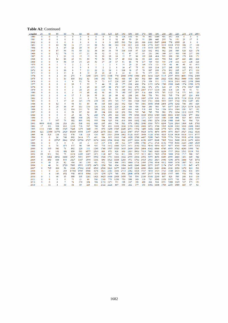
1682
Table A2: Continued

1683
Table A2: Continued

1684
Table A2: Continued

1685
Table A2: Continued
1686
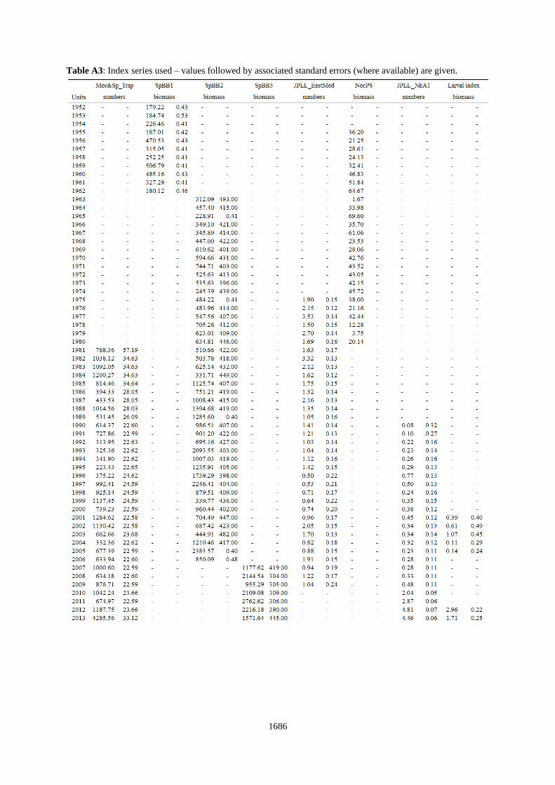
Table A3: Index series used – values followed by associated standard errors (where available) are given.

1687
Appendix B
The Statistical Catch-at-Length Model
The text following sets out the equations and other general specifications of the Statistical Catch at Length
(SCAL) assessment model applied to develop Operating Models (OMs) for the simulation testing, followed by
details of the contributions to the (penalised) log-likelihood function from the different sources of data available
and assumptions concerning the stock-recruitment relationship. Quasi-Newton minimization is then applied to
minimize the total negative log-likelihood function to estimate parameter values (the package AD Model
BuilderTM (Fournier et al. 2011) is used for this purpose). The description below includes more options than used
in this paper, but these have been included here for completeness as they may be used in later extensions.
B.1. Population dynamics
B.1.1 Numbers-at-age
The resource dynamics are modelled by the following set of population dynamics equations:
11,1 yy RN (B1)
ayZ
ayay eNN ,
,1,1
for 1 a m – 2 (B2)
mymy Z
my
Z
mymy eNeNN ,1,
,1,,1
(B3)
where
ayN , is the number of fish of age a at the start of year y (which refers to a calendar year),
m is the maximum age considered (taken to be a plus-group),
yR is the recruitment (number of 1-year-old fish) at the start of year y,
aM denotes the natural mortality rate for fish of age a,
a
f
f
ay
f
yay MSFZ ,, is the total mortality in year y on fish of age a, where
f
yF
is the fishing mortality of a fully selected age class in year y for fishery f, and
f
ayS
, is the commercial selectivity at age a for year y for fishery f.
B.1.2. Recruitment
The number of recruits (i.e. new 1-year olds) at the start of year y is assumed to be related to the spawning stock
size (i.e. the biomass of mature fish) at the mid-point of the preceding year by a Beverton-Holt stock-recruitment
relationship, allowing for annual fluctuation about the deterministic relationship:
)2(
sp
1
sp
12
R
ye
B
BR
y
y
y (B4)
where
and are spawning biomass-recruitment relationship parameters,
y reflects fluctuation about the expected recruitment for year y, which is assumed to be normally
distributed with standard deviation R (which is input in the applications considered here); these
residuals are treated as estimable parameters in the model fitting process. sp
yB is the spawning biomass in year y, computed as:
12,
sp
,
0
,
sp
s
a
TZ
ayay
m
a
ayy eNwfB
(B5)

1688
where
spawning for the stocks under consideration is taken to occur s
T months after the start of the year (here )6sT
and some natural mortality has therefore occurred, sp
,ayw is the mass of fish of age a during spawning, and
ayf , is the proportion of fish of age a that are mature.
B.1.3. Total catch and catches-at-age
The total catch by mass in year y is given by:
ay
Zf
y
f
ayay
m
a
ay
f
ay
m
a
ay
f
y ZeFSNwCwC ay
,,,
0
f
,,
0
f
,,1
(B6)
where f
ayC , is the catch-at-age, i.e. the number of fish of age a, caught in year y by fleet f,
f
ayS , is the commercial selectivity of fleet f (i.e. combination of availability and vulnerability to fishing gear)
at age a for year y; when 1, ayS , the age-class a is said to be fully selected,
f
yF is the proportion of a fully selected age class that is fished by fleet f , and
f
ayw , denotes the selectivity-weighted mid-year weight of fish of age a landed in year y by fleet f, computed
as: f
la
l
lal
f
ly
f
ay SAwSw ,,,,~ (B7)
with
lw is the weight of fish of length l; and
laA , is the proportion of fish of age a that fall in the length group l (i.e., 1, l
laA for all ages).
The matrix laA , is calculated under the assumption that length-at-age is normally distributed about a mean given
by the von Bertalanffy equation, i.e.:
2;1~ a
ta
aoeLNL
(B8)
where
a is the standard deviation of length-at-age a, which is modelled to be proportional to the expected length-at-
age a, i.e.:
ota
a eL
1 (B9)
with fixed here to 0.1 for age 1, 0.2 for age 15 and changing linearly for the intermediate .
Selectivity is estimated as a function of length and then converted to an effective selectivity-at-age:
l
la
f
ly
f
ay ASS ,,, (B10)
B.1.4. Initial conditions
For the first year (y0) considered in the model (here 1950), the numbers-at-age are estimated directly for ages 1
to aest, with a parameter which mimics recent average fishing mortality for ages above aest (aest=4 here), i.e.:
aay NN ,start,0 for
estaa 1 (B11)
and

1689
)1( 11,start,start1
a
M
aa SeNN a for 1 maaest (B12)
))1(1()1( 11,start,start1
m
M
m
M
mm SeSeNN mm
(B13)
B.2. The (penalised) likelihood function
The model is fitted to CPUE and commercial catch-at-length data to estimate model parameters (which may
include residuals about the stock-recruitment function, facilitated through the incorporation of a penalty function
described below). Contributions by each of these to the negative of the (penalised) log-likelihood (- Ln ) are as
follows.
B.2.1 Relative abundance data
The likelihood is calculated assuming that the index observed for a particular fishing fleet is log-normally
distributed about its expected value:
i
y
i
y
i
y
i
y
i
y
i
y IIII ˆnnorexpˆ (B14)
where i
yI is the index of biomass or abundance index for year y for gear/flag combination i,
mZ
ay
i
ay
i
ay
ii
yaeNSwqI
2/
,,,ˆˆ is the corresponding model estimate of biomass or
mZ
ay
i
ay
ii
yaeNSqI
2/
,,ˆˆ is the corresponding model estimate of abundance in numbers, or, in the case of the
larval index: sp
y
ii
y BqI ˆˆ
iq̂ is the constant of proportionality (catchability) for the index series, and
i
y from 2,0 i
yN .
The contribution of the index data to the negative of the log-likelihood function (after removal of constants) is
then given by:
yi
Add
i
i
yi
Add
iL22
2
22i
2nn
(B15)
where i is the standard deviation of the residuals for the logarithm of index i in year y, estimated by its
maximum likelihood value:
y
i
y
ii
yi
i IqIn2
lnln1̂
where ni is the number of data points for index i, and i
Add is the square root of the additional variance for the CPUE series, which can be estimated in the model
fitting procedure but has been set to zero in the applications considered here.
The catchability coefficient iq for index i is estimated by its maximum likelihood value:
y
y
i
yi
i IInqn ˆlnln1ˆ (B16)
The model is fit to the following abundance index series (see Table A4):
1) Mor&Sp_Trap: Moroccan and Spanish (combined) trap (1981-2013)
2) SpBB1: Spanish bait boat (1952-1962)

1690
3) SpBB2: Spanish bait boat (1963-2006)
4) SpBB3: Spanish bait boat (2007-2013)
5) NorPS: Norwegian purse seine (1955-1980)
6) JPLL_EastMed: Japanese longline fishery in east Atl. (south of 40N) and Med. (1975-2009)
7) JPLL_NEA1: Japanese longline fishery in the Northeast Atl. (north of 40N) (1990-2013)
8) Larval index: Western Mediterranean sea (2001-2013)
Note that for the applications considered hear, selectivity at age f
ayS , is year-invariant over the period for which
values of the index are available. More complex formulations are necessary should selectivity-at-age change
during such periods.
The indices' selectivities are taken to be the same as for the overall gear type, i.e.:
1) Mor&Sp_Trap: corresponds to trap
2) SpBB1, SpBB2, and SpBB3 correspond to baitboat
3) NorPS: corresponds to purse seine, and
6) JPLL_EastMed, JPLL_NEA1 and JPLL_NEA2 correspond to longline.
B.2.3. Commercial catches-at-length
The contribution of the catch-at-length data to the negative of the log-likelihood function under the assumption
of an “adjusted” lognormal error distribution (Punt and Kennedy 1997) is given by:
f y l
ff
ly
f
ly
f
ly
f
ly
f
len pnpnppnwL2
len
2
,,,,len
CAL 2/ˆ/n
(B17)
where
'
',,, /l
f
ly
f
ly
f
ly CCp is the observed proportion of fish caught in year y by fleet f that are of length l,
'
',,,ˆ/ˆˆ
l
f
ly
f
ly
f
ly CCp is the model-predicted proportion of fish caught in year y by fleet f that are of length l,
where
a
Zf
lylaay
f
lyayeSANC
2/
,,,,,ˆ (B18)
and f
com is the standard deviation associated with the catch-at-length data, which is estimated in the fitting
procedure by:
y l y l
f
ly
f
ly
f
ay
f pnpnp 1/ˆˆ2
,,,com (B19)
Commercial catches-at-length are grouped with the next length class if the proportion is less than 2%.
The lenw weighting factor may be set to a value less than 1 to downweight the contribution of the catch-at-
length data (which tend to be positively correlated between adjacent length groups) to the overall negative log-
likelihood compared to that of the CPUE data. Here 5.0lenw .
The model is fit to CAL data for each of the five fleets assumed in the model (baitboat, longline, purse seine,
traps, other) (see Table A3).
B.2.4. Stock-recruitment function residuals)
The stock-recruitment residuals are assumed to be log-normally distributed. Thus, the contribution of the
recruitment residuals to the negative of the (now penalised) log-likelihood function is given by:
2
1 1
2
R
2pen 2y
yy
ynL (B20)

1691
where
y is the recruitment residual for year y, which is estimated for year y1 to y2 (see equation (B4)),
R is the standard deviation of the log-residuals, which is input (here R=0.5).
B.3. Estimation of precision
Where quoted, 95% probability interval estimates are based on the Hessian.
B.4. Model parameters
The model input parameters are given in Table B1 below.
B.4.2. Fishing selectivity
Fishing selectivities-at-length are estimated using a four parameters double-logistic form:
122111 111 blabla
leeS (B21)
Details of the fishing selectivities used are shown in Table B2.
Table B1: Input parameters (units are gm, cm and year as appropriate) (length-weight, von Bertalanffy growth,
maturity and natural mortality at age to age 15 from ICCAT, 2012).
Model plus group (m) 15
Length-weight a=0.0000295, b=2.899 (<=100cm) and
a=0.0000196, b=3.009 (>100cm)
von Bertalanffy growth =0.093, Linf=319, t0=-0.97
Maturity-at-age 50% maturity at age 4, 100% maturity at age 5
Natural mortality 1 2-5 6 7 8 9 10+
0.49 0.24 0.20 0.18 0.15 0.13 0.10
Stock-recruitment Beverton-Holt, h=0.98*, R=0.5
* This high value was specified on input rather than estimated in the fit of the model given the absence of any clear trend in the stock-
recruitment plot.
Table B2: Details of the selectivities estimated.
Number of
parameters
estimated
Number of selectivity periods
Bait boat 4x3 Three: 1950-1962, 1963-2006, 2007-2013
Longline 4x1 One
Purse seine 4x5 Three: 1950-1980, 1981-1984, 1985-2001, 2002-2006, 2007-2013
Traps 4x2 Two: 1950-1973, 1974-2013
Other 4x3 Three: 1950-1966, 1967-1984, 1985-2013

1692
Appendix C
Projection methodology
Projections into the future under a specific Candidate Management Procedure (CMP) are evaluated using the
following steps for the Operating Model (OM) under consideration.
Step 1: Begin-year (2014) numbers-at-age
The components of the numbers-at-age vector for each gender and species at the start of 2014 are obtained from
the MLE of an assessment of the resource.
Error is included for numbers-at-ages 1 to 3 because these are poorly estimated in the assessment given limited
information on these year-classes:, i.e.:
aeNN aa
,2014,2014 2
,0 from Ra N
Step 2: Catch
These numbers-at-age are projected one year forward at a time given a catch yC for the year concerned, where
catch is specified by the CMP. This requires specification of how the catch is disaggregated by fleet to obtain f
yC and how future recruitments are generated.
The total TAC recommended by the CMP is divided in fixed proportions among the various fleet, using the 2013
proportions, i.e.:
Baitboat: 3.0%;
Longline: 7.7%;
Purse seine: 63.2%;
Traps: 22.5%
Other: 3.6%
The commercial selectivity functions are taken to stay constant in the projections (i.e. same as 2013).
The numbers-at-age can then be computed for the beginning of the following year (y+1):
11,1 yy RN (C1)
ayZ
ayay eNN ,
,1,1
for 1 a m – 2 (C2)
mymy Z
my
Z
mymy eNeNN ,1,
,1,,1
(C3)
Step 3: Recruitment
Future recruitments are provided by the Beverton-Holt stock-recruitment relationship.
)2(
sp
1
sp
12
R
ye
B
BR
y
y
y (C4)
Log-normal fluctuations are introduced by generating y factors from 2,0 RN .
Step 4: Generate data
The information obtained in Steps 1 to 3 is used to generate values of the indices of abundance (here,
JPLL_NEA and larval index only). The indices are generated from the OM, assuming the same error structures
as in the past.
The index series are generated from model estimates for corresponding mid-year exploitable numbers or
spawning biomass and catchability coefficients, with multiplicative lognormal errors incorporated:
For JPLL_NEA:
iya eeNSqI
mZ
ay
i
ay
ii
y
2/
,,ˆ (C5)
1693
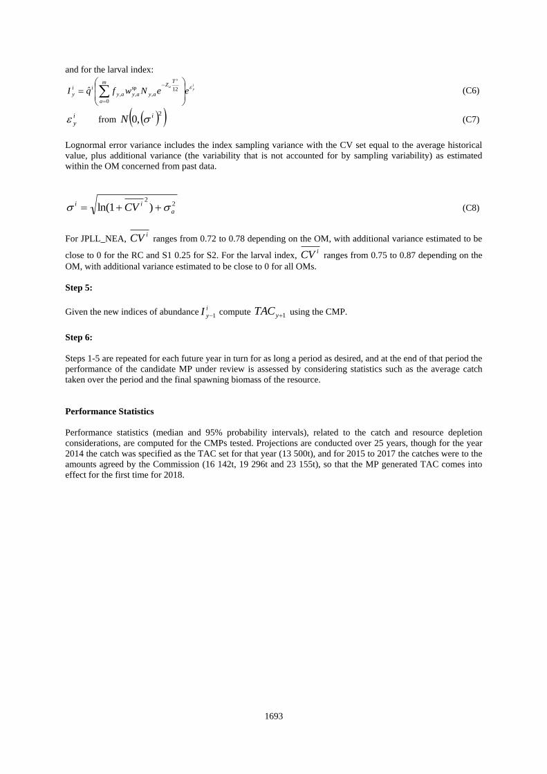
and for the larval index:
iy
s
a
eeNwfqI
TZ
ayay
m
a
ay
ii
y
12,
sp
,
0
,ˆ (C6)
i
y from 2,0 iN (C7)
Lognormal error variance includes the index sampling variance with the CV set equal to the average historical
value, plus additional variance (the variability that is not accounted for by sampling variability) as estimated
within the OM concerned from past data.
22
)1ln( a
ii CV (C8)
For JPLL_NEA, iCV ranges from 0.72 to 0.78 depending on the OM, with additional variance estimated to be
close to 0 for the RC and S1 0.25 for S2. For the larval index, iCV ranges from 0.75 to 0.87 depending on the
OM, with additional variance estimated to be close to 0 for all OMs.
Step 5:
Given the new indices of abundancei
yI 1 compute 1yTAC using the CMP.
Step 6:
Steps 1-5 are repeated for each future year in turn for as long a period as desired, and at the end of that period the
performance of the candidate MP under review is assessed by considering statistics such as the average catch
taken over the period and the final spawning biomass of the resource.
Performance Statistics
Performance statistics (median and 95% probability intervals), related to the catch and resource depletion
considerations, are computed for the CMPs tested. Projections are conducted over 25 years, though for the year
2014 the catch was specified as the TAC set for that year (13 500t), and for 2015 to 2017 the catches were to the
amounts agreed by the Commission (16 142t, 19 296t and 23 155t), so that the MP generated TAC comes into
effect for the first time for 2018.