AN EXPERIMENTAL AND NUMERICAL STUDY OF SUPERCAVITATING …

JOURNAL OF THEORETICAL

AND APPLIED MECHANICS

54, 3, pp. 795-810, Warsaw 2016DOI: 10.15632/jtam-pl.54.3.795

AN EXPERIMENTAL AND NUMERICAL STUDY OF SUPERCAVITATING

FLOWS AROUND AXISYMMETRIC CAVITATORS

S. Morteza Javadpour, Said Farahat

University of Sistan and Baluchestan, Department of Mechanical Engineering, Zahedan, Iran

e-mail: javadpour [email protected]; [email protected]

Hossein Ajam

Ferdowsi University of Mashhad, Department of Mechanical Engineering, Mashhad, Iran; e-mail: [email protected]

Mahmoud Salari

Imam Hossein University, Department of Mechanical Engineering, Tehran, Iran; e-mail: [email protected]

Alireza Hossein Nezhad

University of Sistan and Baluchestan, Department of Mechanical Engineering, Zahedan, Iran

e-mail: [email protected]

It has been shown that developing a supercavitating flow around under-water projectiles hasa significant effect on their drag reduction. As such, it has been a subject of growing attentionin the recent decades. In this paper, a numerical and experimental study of supercavitatingflows around axisymmetric cavitators is presented. The experiments are conducted in asemi-open loop water tunnel. According to the Reynolds-Averaged Navier-Stokes equationsand mass transfer model, a three-component cavitation model is proposed to simulate thecavitating flow. The corresponding governing equations are solved using the finite elementmethod and the mixture Rayleigh-Plesset model. The main objective of this research isto study the effects of some important parameters of these flows such as the cavitationnumber, Reynolds number and conic angle of the cavitators on the drag coefficient as wellas the dimensions of cavities developed around the submerged bodies. A comparison ofthe numerical and experimental results shows that the numerical method is able to predictaccurately the shape parameters of the natural cavitation phenomena such as cavity length,cavity diameter and cavity shape. The results also indicate that the cavitation numberdeclines from 0.32 to 0.25 leading to a 28 percent decrease in the drag coefficient for a30◦ cone cavitator. By increasing the Reynolds number, the cavity length is extended up to322% for a 60◦ cone cavitator.

Keywords: natural cavitation, mass transfer, water tunnel, finite element method, dragcoefficient, axisymmetric cavitators

1. Introduction

Cavitation is the formation of vapor bubbles within a liquid when the liquid pressure falls lessthan the saturated vapor pressure while the fluid temperature remains lower than the boilingtemperature at ambient conditions. Cavitation phenomena are observed in many hydrodynamicmechanical devices such as pumps, turbines, nozzles and marine propellers, which can signi-ficantly influence the performance of these devices. Cavitation may cause negative effects likestructural damages, noise production and power losses in plants, or generates positive effectssuch as drag reduction of underwater moving bodies. However, for military purposes such as tor-pedoes, it is necessary to generate partially- or fully super-cavitating regime to reduce viscousdrag intentionally.The cavitation phenomenon is divided into three stages. The initial form of cavitation is the

bubble stage which has destructive impacts on mechanical systems. Partial cavitation is another

796 S.M. Javadpour et al.

stage in which the cavity region covers some parts of the body. The last stage is supercavita-tion in which size of the produced cavity exceeds the characteristic length of the body. Whensupercavitation occurs, the drag of the bodies surrounded by the cavity is reduced significantly.This is due to reduction in the skin friction drag which depends on viscosity of the near-wallfluid flow, where the vaporous pocket of supercavity surrounds the moving underwater body.Supercavitation can also be divided into natural and ventilated cases. The natural supercavita-tion occurs when free stream velocity rises above a certain limit (U > 45m/s at sea level, whichincreases with submersion depth, or p∞ of the body. This phenomenon can also be achieved bydecreasing the ambient pressure p∞, which is only feasible in cavitation tunnels.

The static hydrodynamic forces and the cavity shape associated with cavitators were modeledby many researchers in the last decades (Logvinovich, 1969, 1980; Kuklinski et al., 2001; Vasinand Paryshev, 2001; Wang et al., 2005; Chen et al., 2006; Chen and Lu, 2008; Deng et al., 2004).

In the recent years, most of the studies related to supercavitating flows have been carriedout numerically. Choi and Ruzzene (2006) explained stability conditions of a supercavitatingvehicle using the finite element method (FEM). Hu and Gao (2010) used the cavitation model ofFluent software to simulate two-phase cavitating flows that contain water and vapor on axisym-metric bodies with disk cavitators. They showed that the vapor volume fraction and thresholdphase-change pressure within the cavity under the same cavitation number gradually ascendsas the Reynolds number increases. Huang et al. (2010) predicted the effects of cavitation over aNACA66 hydrofoil. They combined state equations of the cavitation model with a linear viscousturbulent method of mixed fluids in the Fluent software to simulate a steady cavitating flow.Since most cavitating flows are implemented at high Reynolds numbers and under unsteadyconditions, a suitable turbulence model is required to provide an accurate estimate of cavita-tion. A variety of approaches, such as standard or modified two-equation turbulence models(k − ε, k − ω), have been used to investigate the effects of turbulence on cavitating flows (Wuet al., 2005; Liu et al., 2009, Huang and Wang, 2011; Phoemsapthawee et al., 2012). Large eddysimulation (LES) is another approach used in numerical cavitation modeling recently (Wangand Ostoja-Starzewski, 2007; Huuva, 2008; Liu et al., 2010; Lu et al., 2010). Nouri et al. (2008)used a modified version of the k − ε turbulence model to simulate unsteady behavior of thecavity shedding and the re-entrant flow field. Park and Rhee (2012) studied the standard k − εand realizable k − ε turbulence models by selecting Singhal’s cavitation model at a cavitationnumber of 0.3. They observed that the standard k− ε model was more efficient in capturing there-entrant jet than the realizable k − ε model.In the past decade, several researchers have experimentally investigated supercavitating flows

around the bodies. Most of these studies focused on the shape of generated cavitation, velocityand pressure distributions of the flow field as well as control and stability of supercavitatingvehicles. Lindau et al. (2002) studied a supercavitating flow around a flat disk cavitator. Besi-de general cavitating flows, many studies on supercavitating flows have been undertaken usingexperimental and numerical methods. Experimental methods mainly rely on pressure measure-ments and image processing technology. Lee et al. (2008) studied ventilated supercavitation fora vehicle pitching up and down in the supercavity closed region. Hrubes (2001) studied a su-percavitating flow in underwater projectiles using image production and processing to examineflight behavior, stability mechanism, cavity shape and in-barrel launch characteristics. Recently,Li et al. (2008) studied the cavitating flow by the flow visualization technique using a high-speedcamera. They also measured details of the velocity field by the particle image velocimetry (PIV)to validate the computational models. The shape properties of natural and ventilated superca-vitation on a series of projectile were investigated experimentally by Zhang et al. (2007). Wuand Chahine (2007) studied supercavitation on the back of a simulated projectile and measuredthe properties of the fluid inside the supercavity. Hua et al. (2004) conducted an experimentalstudy on a cavitation tunnel with four axisymmetric bodies at different attack angles. Feng et

An experimental and numerical study of supercavitating flows... 797

al. (2002) studied behavior of a supercavitating and cavitating flow around a conical body ofevolution with and without ventilation at several attack angles. Zhang et al. (2007) performeda series of projectile and closed-loop water-tunnel experiments to study shape properties of na-tural and ventilated supercavitation. Saranjam (2013) did an experimental and numerical studyof cavitation on an underwater moving object based on unsteady effects and dynamic behaviorof the body.Most experimental studies on supercavitation have been performed in a closed-loop water

tunnel with only a few investigations examining the supercavitation flow in an open circuit watertunnel. Also, many experimental studies have been performed to obtain detailed information onthe cavity shape (Fang et al., 2002; Saranjam, 2013, Ji and Luo, 2010; Ahn et al., 2010; Zouet al., 2010). In this study, important supercavitation parameters including the shape of cavity,formation and the drag coefficient of the cavitator are investigated experimentally in a semi-openwater tunnel complemented by a numerical analysis with the CFX software.The paper is organized as follows: first a description of the physical problem followed by an

experimental and numerical analysis is presented. Then, the experimental and computationalresults are presented and discussed. Finally, a summary of the results is given and the relatedconclusions are drawn.

2. Exprimental set-up

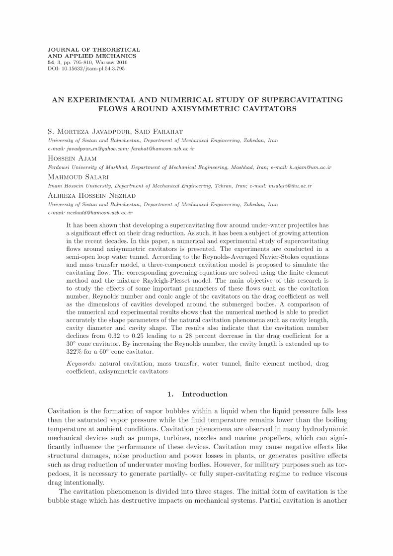
The experiments were conducted in a water tunnel located at the Marine Research Center of Iran.The tunnel is a semi-open loop water tunnel with a maximum velocity of 40m/s. The watertunnel is equipped with a computerized control system, a high frequency data acquisitioningsystem, DAS, and a high-speed camera. A schematic view of the components of the watertunnel is shown in Fig. 1. The body of the model includes cone and cylindrical parts.

Fig. 1. A schematic view of the water tunnel. The figure is not to scale

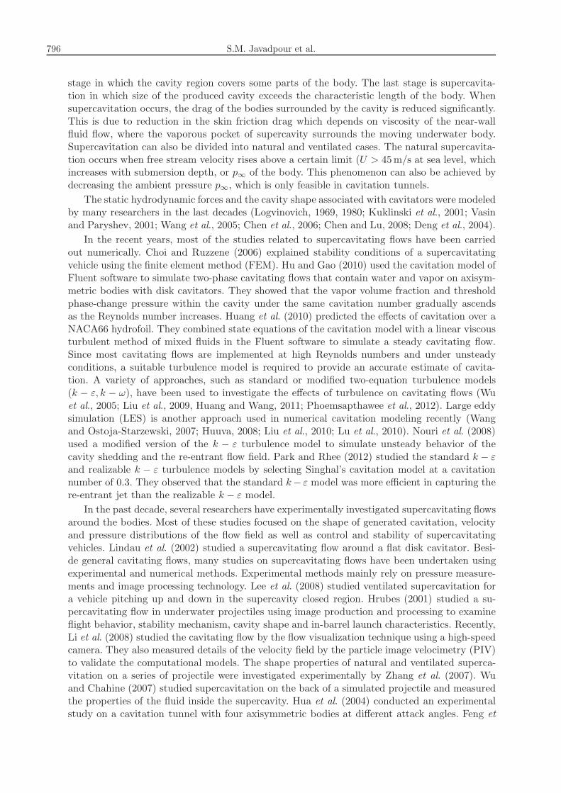
The cavitating flow generated around the symmetric cone was investigated based on theexperimental observations carried out in a water tunnel. Figure 2a shows the test section, wherethe cone cavitator is also placed. The test section has a cylindrical form with diameter of D anda length of 5D (Fig. 2b). The side walls of the test section are made of plexiglas with a highlysmoothed surface. At the outlet of the test section, atmospheric pressure conditions occur andthe fluid flow is discharged into an open surface storage tank. This water tunnel also includesa vertical cylindrical tank as the main water tank which is initially filled with pure water up


to a certain level and then the remaining volume is charged with pressurized air. Depending onthe requested speed, the pressure of the air within the tank is varied. The model is attached toan electronically-load cell mounted outside the test section. The model with the cone cavitatoris shown in Fig. 3. The base diameter of the cone cavitator is 10mm and the cone angles forthe noses are 30◦, 45◦ and 60◦. The cone length of y0 is calculated according to the cone angle.The Reynolds number (Re) based on the diameter of the test section changes from 1120000 to1480000 relative to the stream velocity within the test section.

Fig. 2. (a) Test section of the water tunnel. (b) Dimensions of the test section

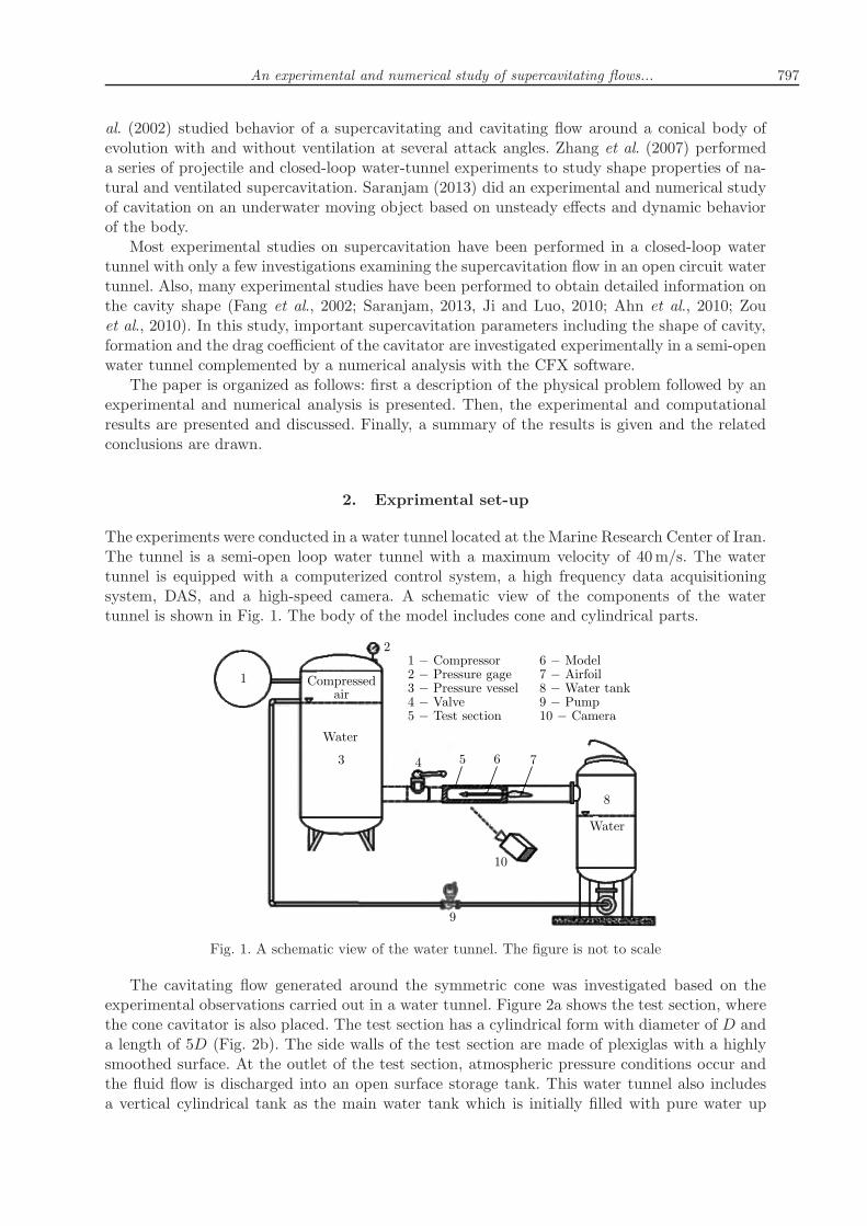
Fig. 3. A schematic view of the model and the position of pressure measurement cavities

The water tunnel was also equipped with some electronic pressure sensors to measure pres-sures in the flow. Five pressure sensors were used to gauge the pressure on the surface of thecylindrical part of the model (Fig. 3) behind the cone cavitator. Two pressure sensors werealso placed inside the test section (P6) and the water tank (P7). The accuracy of sensors was±0.01 bar. The output analog signals of the sensors were converted into digital signals via anA/D card, and the digital results were finally recorded online. It should be noted that the fre-quency of data recording was 1000Hz for all of the sensors in the experiments. The cavitationprofile formed around the cavitator was captured by a high-speed camera with a frame rate of600 fps.

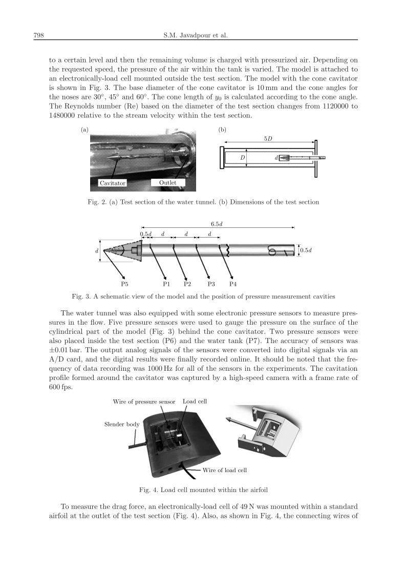
Fig. 4. Load cell mounted within the airfoil

To measure the drag force, an electronically-load cell of 49N was mounted within a standardairfoil at the outlet of the test section (Fig. 4). Also, as shown in Fig. 4, the connecting wires of


the load cell and the pressure sensor were driven out of the water tunnel test section via thatairfoil.

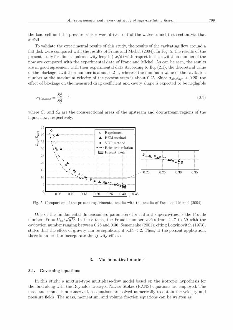
To validate the experimental results of this study, the results of the cavitating flow around aflat disk were compared with the results of Franc and Michel (2004). In Fig. 5, the results of thepresent study for dimensionless cavity length (Lc/d) with respect to the cavitation number of theflow are compared with the experimental data of Franc and Michel. As can be seen, the resultsare in good agreement with their experimental data.According to Eq. (2.1), the theoretical valueof the blockage cavitation number is about 0.211, whereas the minimum value of the cavitationnumber at the maximum velocity of the present tests is about 0.25. Since σblockage < 0.25, theeffect of blockage on the measured drag coefficient and cavity shape is expected to be negligible

σblockage =S2uS2d− 1 (2.1)

where Su and Sd are the cross-sectional areas of the upstream and downstream regions of theliquid flow, respectively.

Fig. 5. Comparison of the present experimental results with the results of Franc and Michel (2004)

One of the fundamental dimensionless parameters for natural supercavities is the Froudenumber, Fr = U∞/

√gD. In these tests, the Froude number varies from 44.7 to 59 with the

cavitation number ranging between 0.25 and 0.36. Semenenko (2001), citing Logvinovitch (1973),states that the effect of gravity can be significant if σvFr < 2. Thus, at the present application,there is no need to incorporate the gravity effects.

3. Mathematical models

3.1. Governing equations

In this study, a mixture-type multiphase-flow model based on the isotropic hypothesis forthe fluid along with the Reynolds averaged Navier-Stokes (RANS) equations are employed. Themass and momentum conservation equations are solved numerically to obtain the velocity andpressure fields. The mass, momentum, and volume fraction equations can be written as


∂ρm∂t+∂

∂xi(ρmui) = 0

∂

∂t(ρmui) +

∂

∂xj(ρmuiuj) = −

∂P

∂xi+∂

∂xj

[

µm(∂ui∂xj+∂uj∂xi

)]

+∂

∂xj(τtij)

∂

∂t(ρvαv) +

∂

∂xi(ρvαvui) = m

− −m+

(3.1)

where αv is the vapor volume fraction, ρv is vapor density, ρl is liquid density and m−, m+ are

mass transfer rates related to evaporation and condensation in cavitation, respectively. Thedensity and dynamic viscosity of the mixture is calculated as

ρm = αvρv + (1− αv)ρl µm = αvµv + (1− αv)µl (3.2)

The non-dimensional parameters of interest in this study, including the cavitation number, dragcoefficient and the Reynolds number, are defined as

σv =P − Pv12ρlU

2∞

Cd =Fd

12ρlU

2∞A

Re =ρlU∞D

µl(3.3)

where Pv, Fd and A are the vapor pressure, drag force and area of test section, respectively.

3.2. Turbulence model

The Reynolds stress can be modeled through the Boussinesq hypothesis according to thefollowing equation

τtij = µt(∂ui∂xj+∂uj∂xi

)

−2

3

(

ρk + µt∂uk∂xk

)

δij (3.4)

The standard k−ε turbulence model,which is based on the Boussinesq hypothesis with transportequations for the turbulent kinetic energy k and its dissipation rate ε is adopted for the turbu-lence closure. The turbulent viscosity µt, is computed by combining k and ε as µt = (ρmCµk

2)/ε,and the turbulence kinetic energy and its rate of dissipation are obtained from the transportequations as follows

∂(ρmk)

∂t+∂(ρmujk)

∂xj=∂

∂xj

[(

µ+µtσk

) ∂k

∂xj

]

+Gk +Gb − ρε− YM

∂(ρmε)

∂t+∂(ρmuj)

∂xj=∂

∂xj

[(

µ+µtσε

) ∂ε

∂xj

]

+Cε1ε

k(Gk + C3εGb)−Cε2ρ

ε2

k

(3.5)

where Cµ is an empirical constant (0.09). Here, the model constants Cε1, Cε2, σk and σε are 1.44,1.92, 1.0 and 1.3, respectively. The turbulent viscosity is used to calculate the Reynolds stressesto close the momentum equations. To model the flow close to the wall, a scalable wall-functionapproach has been adopted. The finite volume method is employed to discretize the integral-differential equations. The second-order upwind scheme is applied to discretize the turbulenttransportation equations.

3.3. Cavitation model

To model the cavitating flows, the two phases of liquid and vapor as well as the phasetransition mechanism between them need to be specified. In this study, a “two-phase mixture”approach is introduced by the local vapor volume, which has the spatial and temporal variationof the vapor function, as described by the transport equation together with the source terms forthe mass transfer rate between the two phases. Numerical models of cavitation differ in terms of


the mass transfer term m. The most common semi analytical models are the Singhal cavitationmodel (2002), Merkle model (1998), Schnerr and Sauer model (2001) and Kunz model (1999).In the present study, the cavitation model developed by Singhal et al. (2002) is used. Thesource terms included in the transport equation define vapor generation (liquid evaporation)and vapor condensation respectively. The source terms are functions of local flow conditions(static pressure and velocity) and fluid properties (liquid and vapor phase densities, saturationpressure and liquid vapor surface tension). The source terms are derived from the Rayleigh-Plesset equation, where high-order terms and viscosity terms can be found according to Singhalet al. (2002)

m− = CevapVchσρlρv

√

2

3

pv − pρl

ρlαlρm

m+ = CcondVchσρlρv

√

2

3

p− pvρl

ρvαvρm

(3.6)

where Cevap = 0.02, Ccond = 0.01 and Vch =√k, pv, σ and k denote the saturated pressure of

liquid, surface tension and turbulence energy, respectively.

4. Numerical method

Numerical simulation (Ansys CFX 14) can be used to detect cavitation in the cavitation flowaround the cone cavitator. It is important to note that ANSYS CFX uses the CV-FEM (controlvolume-finite element) method, with the latter having superior performance with the hexahedralmesh than with the tetrahedral one, which tends to degrade the computing efficiency.Given the application of the CV-FEM method in ANSYS CFX 14, the linearized momentum

and mass equations are solved simultaneously with an algebraic multi-grid method based on theadditive correction multi-grid strategy. The implementation of this strategy in ANSYS CFX hasbeen found to offer a robust and efficient prediction of the cavitation in pumps (Athavale et al.,2002; Pouffary et al., 2003). The high resolution scheme is adopted in space discretization tosolve the differential equation as it has the second-order space accuracy.

5. Computational domain and boundary condition

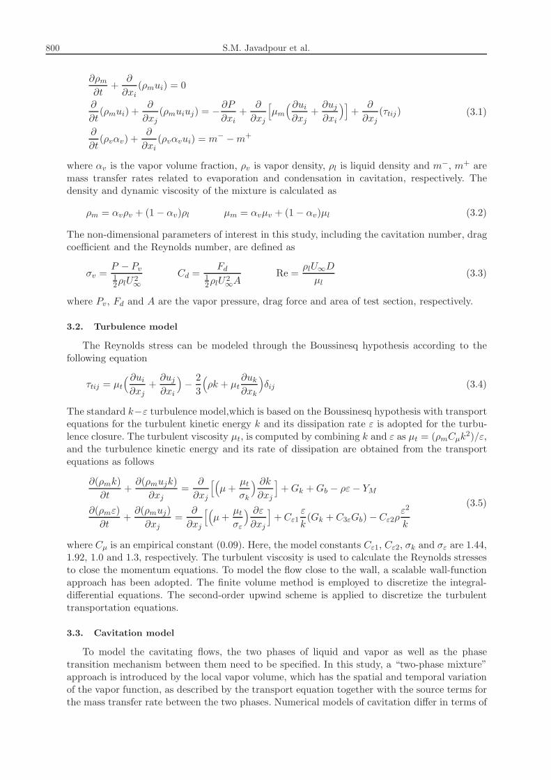
The domain of the problem and boundary conditions are shown in Fig. 6.The boundary conditions in the water tunnel are as follows:

• At the inlet, the velocity components, volume fractions, turbulence intensity and the lengthscale are specified.

• At the outlet, the pressure, volume fractions, turbulence intensity and the length scale arespecified.

• The wall of the water tunnel and cavitator is assumed to be in no slip conditions.

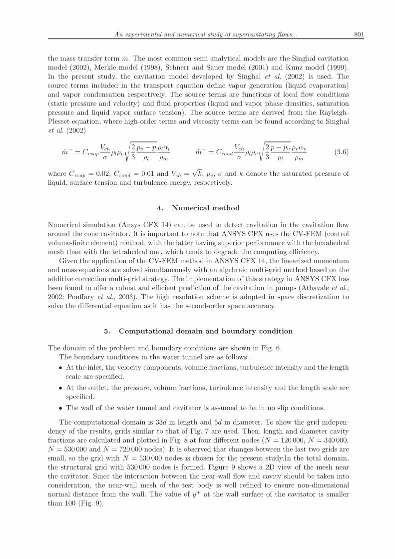
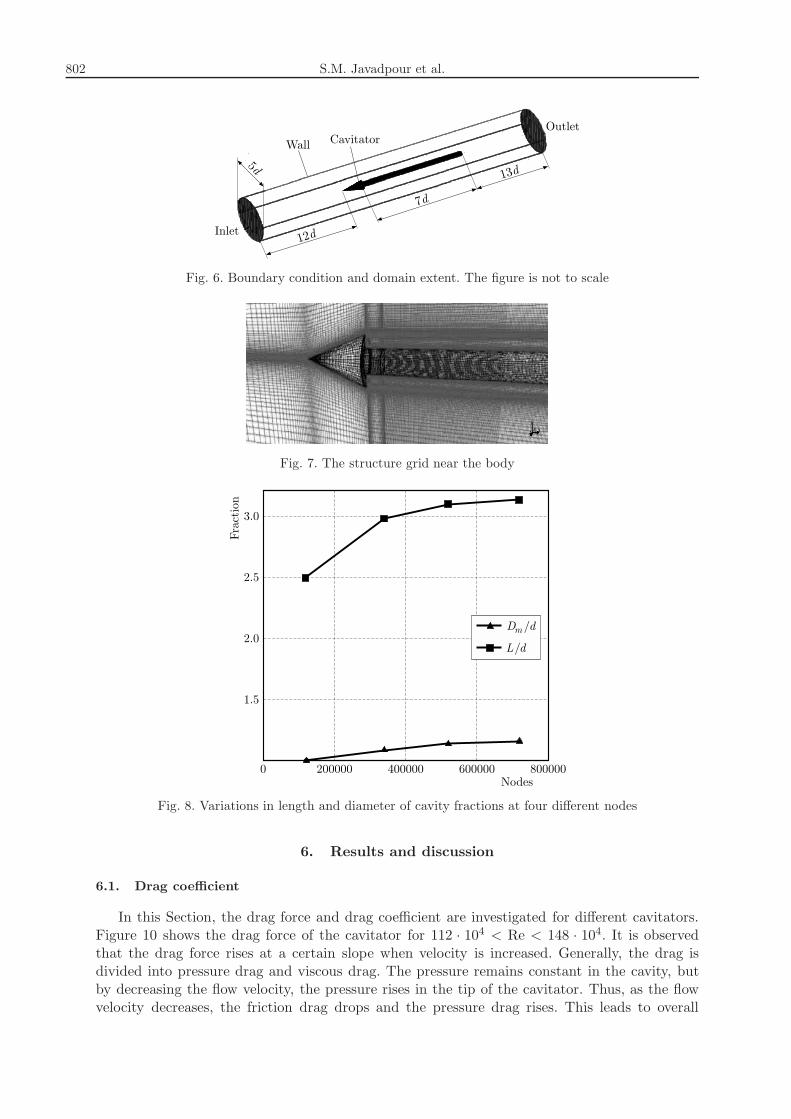
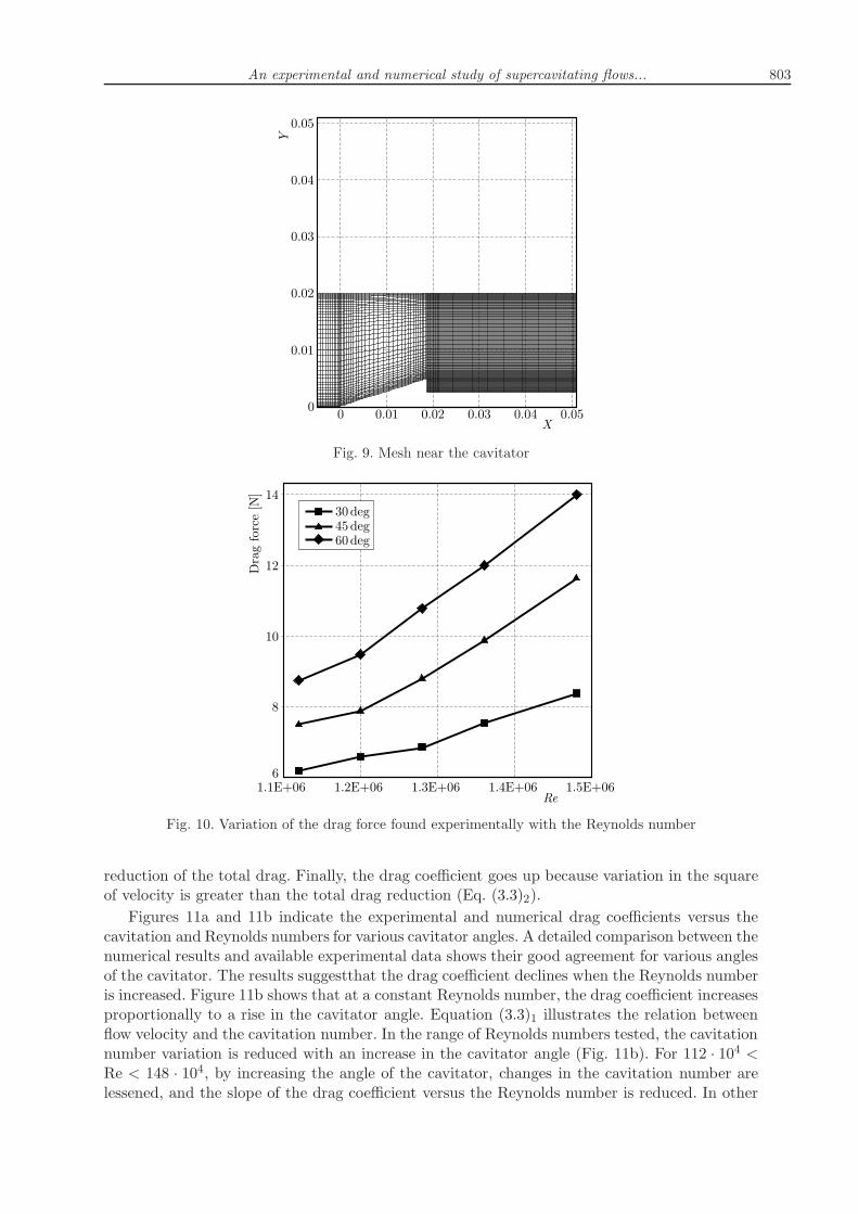
The computational domain is 33d in length and 5d in diameter. To show the grid indepen-dency of the results, grids similar to that of Fig. 7 are used. Then, length and diameter cavityfractions are calculated and plotted in Fig. 8 at four different nodes (N = 120 000, N = 340 000,N = 530 000 and N = 720 000 nodes). It is observed that changes between the last two grids aresmall, so the grid with N = 530 000 nodes is chosen for the present study.In the total domain,the structural grid with 530 000 nodes is formed. Figure 9 shows a 2D view of the mesh nearthe cavitator. Since the interaction between the near-wall flow and cavity should be taken intoconsideration, the near-wall mesh of the test body is well refined to ensure non-dimensionalnormal distance from the wall. The value of y+ at the wall surface of the cavitator is smallerthan 100 (Fig. 9).


Fig. 6. Boundary condition and domain extent. The figure is not to scale

Fig. 7. The structure grid near the body

Fig. 8. Variations in length and diameter of cavity fractions at four different nodes

6. Results and discussion

6.1. Drag coefficient

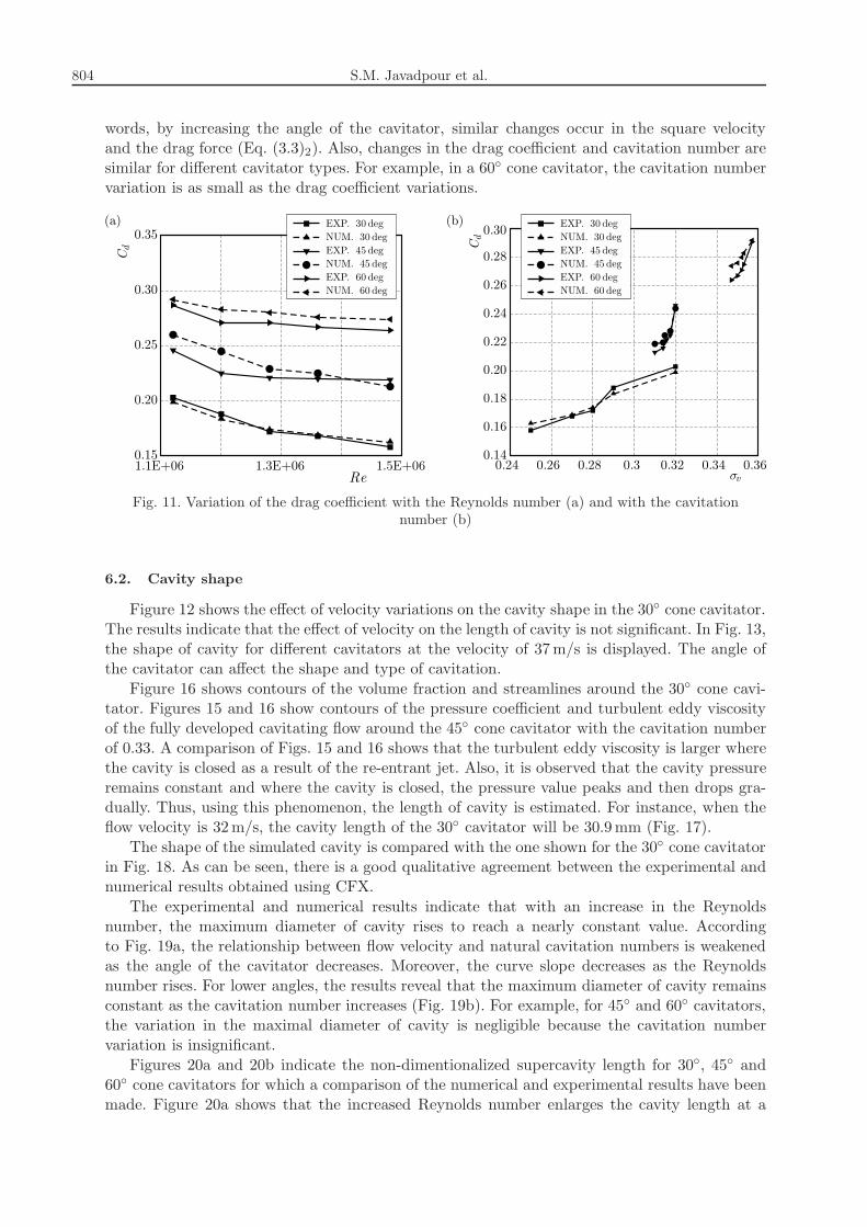
In this Section, the drag force and drag coefficient are investigated for different cavitators.Figure 10 shows the drag force of the cavitator for 112 · 104 < Re < 148 · 104. It is observedthat the drag force rises at a certain slope when velocity is increased. Generally, the drag isdivided into pressure drag and viscous drag. The pressure remains constant in the cavity, butby decreasing the flow velocity, the pressure rises in the tip of the cavitator. Thus, as the flowvelocity decreases, the friction drag drops and the pressure drag rises. This leads to overall


Fig. 9. Mesh near the cavitator

Fig. 10. Variation of the drag force found experimentally with the Reynolds number

reduction of the total drag. Finally, the drag coefficient goes up because variation in the squareof velocity is greater than the total drag reduction (Eq. (3.3)2).

Figures 11a and 11b indicate the experimental and numerical drag coefficients versus thecavitation and Reynolds numbers for various cavitator angles. A detailed comparison between thenumerical results and available experimental data shows their good agreement for various anglesof the cavitator. The results suggestthat the drag coefficient declines when the Reynolds numberis increased. Figure 11b shows that at a constant Reynolds number, the drag coefficient increasesproportionally to a rise in the cavitator angle. Equation (3.3)1 illustrates the relation betweenflow velocity and the cavitation number. In the range of Reynolds numbers tested, the cavitationnumber variation is reduced with an increase in the cavitator angle (Fig. 11b). For 112 · 104 <Re < 148 · 104, by increasing the angle of the cavitator, changes in the cavitation number arelessened, and the slope of the drag coefficient versus the Reynolds number is reduced. In other


words, by increasing the angle of the cavitator, similar changes occur in the square velocityand the drag force (Eq. (3.3)2). Also, changes in the drag coefficient and cavitation number aresimilar for different cavitator types. For example, in a 60◦ cone cavitator, the cavitation numbervariation is as small as the drag coefficient variations.

Fig. 11. Variation of the drag coefficient with the Reynolds number (a) and with the cavitationnumber (b)

6.2. Cavity shape

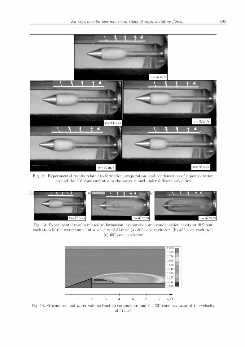
Figure 12 shows the effect of velocity variations on the cavity shape in the 30◦ cone cavitator.The results indicate that the effect of velocity on the length of cavity is not significant. In Fig. 13,the shape of cavity for different cavitators at the velocity of 37m/s is displayed. The angle ofthe cavitator can affect the shape and type of cavitation.

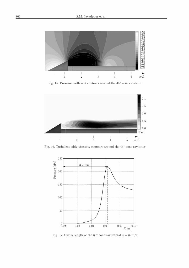
Figure 16 shows contours of the volume fraction and streamlines around the 30◦ cone cavi-tator. Figures 15 and 16 show contours of the pressure coefficient and turbulent eddy viscosityof the fully developed cavitating flow around the 45◦ cone cavitator with the cavitation numberof 0.33. A comparison of Figs. 15 and 16 shows that the turbulent eddy viscosity is larger wherethe cavity is closed as a result of the re-entrant jet. Also, it is observed that the cavity pressureremains constant and where the cavity is closed, the pressure value peaks and then drops gra-dually. Thus, using this phenomenon, the length of cavity is estimated. For instance, when theflow velocity is 32m/s, the cavity length of the 30◦ cavitator will be 30.9mm (Fig. 17).

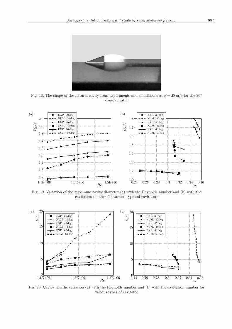
The shape of the simulated cavity is compared with the one shown for the 30◦ cone cavitatorin Fig. 18. As can be seen, there is a good qualitative agreement between the experimental andnumerical results obtained using CFX.

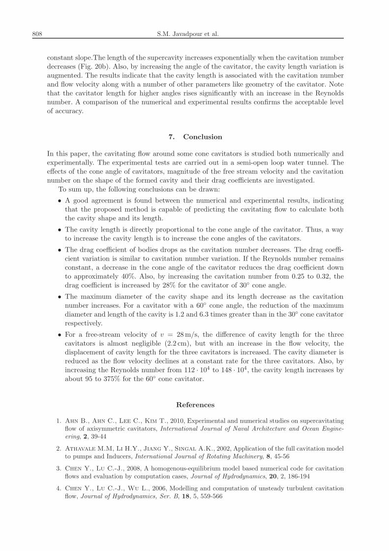
The experimental and numerical results indicate that with an increase in the Reynoldsnumber, the maximum diameter of cavity rises to reach a nearly constant value. Accordingto Fig. 19a, the relationship between flow velocity and natural cavitation numbers is weakenedas the angle of the cavitator decreases. Moreover, the curve slope decreases as the Reynoldsnumber rises. For lower angles, the results reveal that the maximum diameter of cavity remainsconstant as the cavitation number increases (Fig. 19b). For example, for 45◦ and 60◦ cavitators,the variation in the maximal diameter of cavity is negligible because the cavitation numbervariation is insignificant.

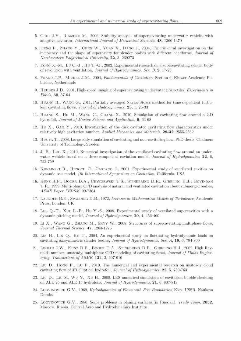
Figures 20a and 20b indicate the non-dimentionalized supercavity length for 30◦, 45◦ and60◦ cone cavitators for which a comparison of the numerical and experimental results have beenmade. Figure 20a shows that the increased Reynolds number enlarges the cavity length at a


Fig. 12. Experimental results related to formation, evaporation, and condensation of supercavitationaround the 30◦ cone cavitator in the water tunnel under different velocities

Fig. 13. Experimental results related to formation, evaporation and condensation cavity at differentcavitators in the water tunnel at a velocity of 37m/s; (a) 30◦ cone cavitator, (b) 45◦ cone cavitator,

(c) 60◦ cone cavitator

Fig. 14. Streamlines and water volume fraction contours around the 30◦ cone cavitator at the velocityof 37m/s


Fig. 15. Pressure coefficient contours around the 45◦ cone cavitator

Fig. 16. Turbulent eddy viscosity contours around the 45◦ cone cavitator

Fig. 17. Cavity length of the 30◦ cone cavitatorat v = 32m/s


Fig. 18. The shape of the natural cavity from experiments and simulations at v = 28m/s for the 30◦

conecavitator

Fig. 19. Variation of the maximum cavity diameter (a) with the Reynolds number and (b) with thecavitation number for various types of cavitators

Fig. 20. Cavity lengths variation (a) with the Reynolds number and (b) with the cavitation number forvarious types of cavitator


constant slope.The length of the supercavity increases exponentially when the cavitation numberdecreases (Fig. 20b). Also, by increasing the angle of the cavitator, the cavity length variation isaugmented. The results indicate that the cavity length is associated with the cavitation numberand flow velocity along with a number of other parameters like geometry of the cavitator. Notethat the cavitator length for higher angles rises significantly with an increase in the Reynoldsnumber. A comparison of the numerical and experimental results confirms the acceptable levelof accuracy.

7. Conclusion

In this paper, the cavitating flow around some cone cavitators is studied both numerically andexperimentally. The experimental tests are carried out in a semi-open loop water tunnel. Theeffects of the cone angle of cavitators, magnitude of the free stream velocity and the cavitationnumber on the shape of the formed cavity and their drag coefficients are investigated.

To sum up, the following conclusions can be drawn:

• A good agreement is found between the numerical and experimental results, indicatingthat the proposed method is capable of predicting the cavitating flow to calculate boththe cavity shape and its length.

• The cavity length is directly proportional to the cone angle of the cavitator. Thus, a wayto increase the cavity length is to increase the cone angles of the cavitators.

• The drag coefficient of bodies drops as the cavitation number decreases. The drag coeffi-cient variation is similar to cavitation number variation. If the Reynolds number remainsconstant, a decrease in the cone angle of the cavitator reduces the drag coefficient downto approximately 40%. Also, by increasing the cavitation number from 0.25 to 0.32, thedrag coefficient is increased by 28% for the cavitator of 30◦ cone angle.

• The maximum diameter of the cavity shape and its length decrease as the cavitationnumber increases. For a cavitator with a 60◦ cone angle, the reduction of the maximumdiameter and length of the cavity is 1.2 and 6.3 times greater than in the 30◦ cone cavitatorrespectively.

• For a free-stream velocity of v = 28m/s, the difference of cavity length for the threecavitators is almost negligible (2.2 cm), but with an increase in the flow velocity, thedisplacement of cavity length for the three cavitators is increased. The cavity diameter isreduced as the flow velocity declines at a constant rate for the three cavitators. Also, byincreasing the Reynolds number from 112 · 104 to 148 · 104, the cavity length increases byabout 95 to 375% for the 60◦ cone cavitator.

References

1. Ahn B., Ahn C., Lee C., Kim T., 2010, Experimental and numerical studies on supercavitatingflow of axisymmetric cavitators, International Journal of Naval Architecture and Ocean Engine-ering, 2, 39-44

2. Athavale M.M, Li H.Y., Jiang Y., Singal A.K., 2002, Application of the full cavitation modelto pumps and Inducers, International Journal of Rotating Machinery, 8, 45-56

3. Chen Y., Lu C.-J., 2008, A homogenous-equilibrium model based numerical code for cavitationflows and evaluation by computation cases, Journal of Hydrodynamics, 20, 2, 186-194

4. Chen Y., Lu C.-J., Wu L., 2006, Modelling and computation of unsteady turbulent cavitationflow, Journal of Hydrodynamics, Ser. B, 18, 5, 559-566


5. Choi J.Y., Ruzzene M., 2006. Stability analysis of supercavitating underwater vehicles withadaptive cavitator, International Journal of Mechanical Sciences, 48, 1360-1370

6. Deng F., Zhang Y., Chen W., Yuan X., Dang J., 2004, Experimental investigation on theincipiency and the shape of supercavity for slender bodies with different headforms, Journal ofNorthwestern Polytechnical University, 22, 3, 269273

7. Fong X.-M., Lu C.-J., Hu T.-Q., 2002, Experimental research on a supercavitating slender bodyof revolution with ventilation, Journal of Hydrodynamics, Ser. B, 2, 17-23

8. Franc J.P., Michel J.M., 2004, Fundamentals of Cavitation, Section 6, Kluwer Academic Pu-blisher, Netherlands

9. Hrubes J.D., 2001, High-speed imaging of supercavitating underwater projectiles, Experiments inFluids, 30, 57-64

10. Huang B., Wang G., 2011, Partially averaged Navier-Stokes method for time-dependent turbu-lent cavitating flows, Journal of Hydrodynamics, 23, 1, 26-33

11. Huang S., He M., Wang C., Chang X., 2010, Simulation of cavitating flow around a 2-Dhydrofoil, Journal of Marine Science and Application, 9, 63-68

12. Hu X., Gao Y., 2010, Investigation of the disk cavitator cavitating flow characteristics underrelatively high cavitation number, Applied Mechanics and Materials, 29-32, 2555-2562

13. Huuva T., 2008, Large eddy simulation of cavitating and non-cavitating flow, PhD thesis, ChalmersUniversity of Technology, Sweden

14. Ji B., Luo X., 2010, Numerical investigation of the ventilated cavitating flow around an under-water wehicle based on a three-component caviation model, Journal of Hydrodynamics, 22, 6,753-759

15. Kuklinski R., Henoch C., Castano J., 2001, Experimental study of ventilated cavities ondynamic test model, 4th International Symposium on Cavitation, California, USA

16. Kunz R.F., Boger D.A., Chyczewski T.S., Stinebring D.R., Gibeling H.J., GovindanT.R., 1999. Multi-phase CFD analysis of natural and ventilated cavitation about submerged bodies,ASME Paper FEDSM, 99-7364

17. Launder B.E., Spalding D.B., 1972, Lectures in Mathematical Models of Turbulence, AcademicPress, London, UK

18. Lee Q.-T., Xue L.-P., He Y.-S., 2008, Experimental study of ventilated supercavities with adynamic pitching model, Journal of Hydrodynamics, 20, 4, 456-460

19. Li X., Wang G., Zhang M., Shyy W., 2008, Structures of supercavitating multiphase flows,Journal Thermal Science, 47, 1263-1275

20. Lin H., Lin Q., Hu T., 2004, An experimental study on fluctuating hydrodynamic loads oncavitating axisymmetric slender bodies, Journal of Hydrodynamics, Ser. A, 19, 6, 794-800

21. Lindau J.W., Kunz R.F., Boger D.A., Stinebring D.R., Gibeling H.J., 2002, High Rey-nolds number, unsteady, multiphase CFD modeling of cavitating flows, Journal of Fluids Engine-ering, Transactions of ASME, 124, 3, 607-616

22. Liu D., Hong F., Lu F., 2010, The numerical and experimental research on unsteady cloudcavitating flow of 3D elliptical hydrofoil, Journal of Hydrodynamics, 22, 5, 759-763

23. Liu D., Liu S., Wu Y., Xu H., 2009, LES numerical simulation of cavitation bubble sheddingon ALE 25 and ALE 15 hydrofoils, Journal of Hydrodynamics, 21, 6, 807-813

24. Logvinovich G.V., 1969, Hydrodynamics of Flows with Free Boundaries, Kiev, USSR, NaukovaDumka

25. Logvinovich G.V., 1980, Some problems in planing surfaces (in Russian), Trudy Tsagi, 2052,Moscow, Russia, Central Aero and Hydrodynamics Institute


26. Lu N., Bensow R.E., Bark G., 2010, LES of unsteady cavitation on the delft twisted foil,Journal of Hydrodynamics, Ser. B, 22, 5, 784-791

27. Merkle C.L., Feng J., Buelow P.E.O., 1998, Computational modeling of the dynamics ofsheet cavitation, Proceeding of the 3rd International Symposium on Cavitation (CAV98), Grenoble,France

28. Nouri N.M., Shienejad A., Eslamdoost A., 2008, Multi phase computational fluid dyna-mics modeling of cavitating flows over axisymmetric head-forms, IUST International Journal ofEngineering Science, 19, 1/5, 71-81

29. Park S., Rhee S.H., 2012, Computational analysis of turbulent supercavitating flow around atwodimensional wedge-shaped cavitator geometry, Computers and Fluids, 70, 73-85

30. Phoemsapthawee S., Leroux J., Kerampran S., Laurens J., 2012, Implementation of atranspiration velocity based cavitation model within a RANS solver, European Journal of Mecha-nics B/Fluids, 32, 45-51

31. Pouffary B., Fortes-Patella R., Reboud J.L., 2003, Numerical simulation of cavitating flowaround a 2D hydrofoil: a barotropic approach, Fith International Symposium on Cavitation, Osaka,Japan

32. Saranjam B., 2013, Experimental and numerical investigation of an unsteady supercavitatingmoving body, Ocean Engineering, 59, 9-14

33. Schnerr G., Sauer J., 2001, Physical and numerical modeling of unsteady cavitation dynamics,4th International Conference on Multiphase Flows, New Orleans, USA

34. Semenenko V.N., 2001, Dynamic processes of supercavitation and computer simulation, RTOAVT Lecture Series on Supercavitatingows at VKI

35. Singhal A.K., Athavale M.M., Li H., Jiang Y., 2002, Mathematical basis and validation ofthe full cavitation model, Journal of Fluids Enginnering, 124, 617-624

36. Vasin A.D., Paryshev E.V., 2001, Immersion of a cylinder in a fluid through a cylindrical freesurface, Journal of Fluid Dynamics, 36, 2, 168-177

37. Wang G., Ostoja-Starzewski M., 2007, Large eddy simulation of a sheet/cloud cavitation ona NACA 0015 hydrofoil, Applied Mathematical Modelling, 31, 3, 417-447

38. Wang H., Zhang J., Wei Y., Yu K., Jia L., 2005, Study on relations between cavity form andtypical cavitator parameters, Journal of Hydrodynamics, Ser. A, 20, 2, 251-257

39. Wu J., Wang G., Shyy W., 2005, Time-dependent turbulent cavitating flow computation withinterfacial transport and filter-based models, International Journal for Numerical Methods in Flu-ids, 49, 739-746

40. Wu X., Chahine G.L., 2007, Characterization of the content of the cavity behind a high-speedsupercavitating body, Journal of Fluids Enginnering, 45, 129-136

41. Zhang X.-W., Wei Y.-J., Zhang J.-Z., Chen Y., Yu K.-P., 2007, Experimental research onthe shape characters of natural and ventilated supercavitation, Journal of Hydrodynamics, Ser. B,19, 5, 564-571

42. Zou W., Yu K., Wan X., 2010, Research on the gas-leakage rate of unsteady ventilated super-cavity, Journal of Hydrodynamics, 22, 5, 778-783

Manuscript received June 4, 2015; accepted for print November 26, 2015

Documents

AN EXPERIMENTAL AND NUMERICAL STUDY OF SUPERCAVITATING …