Embed Size (px)
Citation preview

ECONOMIC GROWTH CENTERYALE UNIVERSITY
P.O. Box 208269New Haven, CT 06520-8269
http://www.econ.yale.edu/~egcenter/
CENTER DISCUSSION PAPER NO. 860
AN EQUILIBRIUM MODEL OF SORTING IN AN URBAN HOUSINGMARKET: THE CAUSES AND CONSEQUENCES OF RESIDENTIAL
SEGREGATION
Patrick BayerYale University
Robert McMillanUniversity of Toronto
Kim RuebenPublic Policy Institute of California
July 2003
Notes: Center Discussion Papers are preliminary materials circulated to stimulate discussions and criticalcomments.
The authors would like to thank Fernando Ferreira (University of California, Berkeley) for outstanding research assistance andPedro Cerdan and Jackie Chou for help in assembling the data set. We are grateful to Joe Altonji, Pat Bajari, Steve Berry,Gregory Besharov, Greg Crawford, David Cutler, Dennis Epple, James Heckman, Vernon Henderson, Phil Leslie, Enrico Moretti,Robert Moffitt, Tom Nechyba, Steve Ross, Holger Sieg, Kerry Smith, Jon Sonstelie, Chris Taber, Chris Timmins, Chris Udry,Jacob Vigdor, and participants at the meetings of the AEA 2002, ERC Conference on Empirical Economic Models of PricingValuation and Resource Allocation 2002, IRP Summer Workshop 2001, NBER Summer Institute 2003, Public Economic Theory2003, and SITE 2001, SIEPR Workshop on Equilibrium Modeling Approaches, and seminars at Brown, Chicago, Colorado,Duke, Johns Hopkins, Northwestern, NYU, PPIC, Toronto, UC Berkeley, UC Irvine, UCLA, and Yale for providing manyvaluable comments and suggestions. This research was conducted at the California Census Research Data Center; our thanksto the CCRDC, and to Ritch Milby in particular. We gratefully acknowledge the financial support for this project providedby the National Science Foundation under grant SES-0137289 and the Public Policy Institute of California.
This paper can be downloaded without charge from the Social Science Research Network electronic libraryat: http://ssrn.com/abstract=429241
An index to papers in the Economic Growth Center Discussion Paper Series is located at: http://www.econ.yale.edu/~egcenter/research.htm

An Equilibrium Model of Sorting in an Urban Housing Market: The Causes and Consequences of Residential Segregation
Patrick Bayer, Robert McMillan, and Kim Rueben
Abstract
This paper presents a new equilibrium framework for analyzing economic and policy questions related to the
sorting of households within a large metropolitan area. We estimate the model using restricted-access Census data
that precisely characterize residential and employment locations for households the San Francisco Bay Area,
yielding accurate measures of preferences for a wide variety of housing and neighborhood attributes across
different types of household. We use these estimates to explore the causes and consequences of racial
segregation in general equilibrium. Our results indicate that, given the preference structure of households in the
Bay Area, the elimination of racial differences in income and wealth would significantly increase the residential
segregation of each major racial group, as the equalization of income leads, for example, to the formation of new
wealthy, segregated Black and Hispanic neighborhoods. We also provide evidence that sorting on the basis of race
itself (whether driven by preferences or discrimination) leads to large reductions in the consumption of housing,
public safety, and school quality by Black and Hispanic households.
JEL Classification: H0, J7, R0, R2
Keywords: Segregation, Sorting, Housing Markets, Locational Equilibrium, Residential Choice, Discrete
Choice

2
1 INTRODUCTION
A number of important features of the landscape of an urban housing market are determined by
the way that households sort among its neighborhoods. This sorting affects residential stratification on
the basis of race, income, and other family attributes, the congestion of the transportation network, and
the distribution of school quality, crime, property tax bases, and housing prices throughout the urban area.
It also has important welfare implications. A full understanding of these implications requires knowledge
of the preferences of the heterogeneous households in the metropolitan region and a model that describes
how these preferences aggregate to form an equilibrium. The primary goal of this paper is to provide
these necessary components.
To that end, we develop an equilibrium model of sorting in an urban housing market and provide
a general strategy for identifying preferences in the presence of social interactions in the location
decision. Building on McFadden’s (1978) discrete choice framework, our model allows households to
have preferences for a wide variety of housing and neighborhood attributes, including many that depend
explicitly on the way that households sort across neighborhoods in equilibrium (e.g. the quality of local
schools, the neighborhood crime rate, and the sociodemographic composition of the neighborhood). Each
household’s preferences are allowed to vary with its own characteristics, including its wealth, income,
education, race, employment location (taken as given), and family composition. The model also provides
a well-defined characterization of how these preferences aggregate to determine the equilibrium in an
urban housing market; under a set of reasonable assumptions, we demonstrate that a sorting equilibrium
always exists in this framework.
The model is estimated using newly available, restricted Census micro-data that provide precise
geographic information on the residential locations of a quarter of a million households in the San
Francisco Bay Area in 1990. Because the sorting equilibrium is not generically unique, we develop an
estimation strategy that permits estimation in the presence of multiple equilibria, exploiting the fact that in
any equilibrium, each household chooses its location optimally conditional on the decisions made by the
other households in the metropolitan region. This strategy does not require us to compute the equilibrium
as part of the estimation procedure, thereby allowing the estimation of hundreds of heterogeneity
parameters in a computationally feasible manner.
Following Berry, Levinsohn, and Pakes (1995), we allow explicitly for unobserved differences in
the quality of houses and neighborhoods. In so doing, we bring an important endogeneity problem to the

3
forefront of the analysis – namely that the value (or rent) of a house and any other neighborhood attributes
determined by the sorting of households are likely to be highly correlated with unobserved house and
neighborhood attributes. And we provide a general strategy for identifying the model in the face of this
endogeneity problem, developing an appropriate set of instruments for endogenous choice characteristics.
We show that instruments rise naturally out of the logic of the choice model itself. Because each
household’s location decision is affected by the full set of available alternatives, the housing prices and
sociodemographic composition of any particular neighborhood will be partly dependent on the wider
availability of choices in the urban housing market. In particular, characteristics of the housing stock and
land use in surrounding neighborhoods can be expected to influence, through the market equilibrium,
prices and sociodemographics of a given neighborhood. At the same time, as long as the surrounding
neighborhoods are sufficiently distant, it is unlikely that their fixed characteristics are correlated with the
unobserved features of a given neighborhood that affect household utility, allowing them to serve as valid
instruments.
The estimated model yields precise measures of the full set of preference parameters which, along
with the characterization of how these preferences aggregate to determine the market equilibrium, can be
used to explore a wide variety of economic questions concerning sorting in the urban housing market.
The model is particularly useful for carrying out urban policy analysis, providing a way to measure the
general equilibrium effects of a policy in terms of its impact on the sociodemographic composition, house
values (and rents), school quality, and crime rates of each neighborhood of the metropolitan region, its
impact on the intensity of usage of the transportation network, and clear measures of the policy’s
distributional consequences in terms of income, race, and other household attributes.
Relation to Previous Models of Sorting in an Urban Housing Market
Our framework draws on two main lines of research in the empirical urban economics literature.
Following the seminal work of McFadden (1973, 1978), many researchers have used a discrete choice
framework to study residential location decisions, as this framework provides a natural way to estimate
heterogeneous preferences for housing and neighborhood attributes.1 Relative to this literature, the key
contribution of our approach is that we explicitly control for the fact that housing prices and
neighborhood sociodemographic characteristics are determined as part of the sorting equilibrium, both 1 Important applications of this framework can be found in Anas (1982), Anas and Chu (1984), Quigley (1985), and Gabriel and Rosenthal (1989), Nechyba and Strauss (1998), and Duncombe, Robbins, and Wolf (1999).

4
when estimating the model and conducting counterfactual simulations.2 In formally characterizing the
sorting equilibrium, we build on a vast theoretical literature in urban and public economics3 and most
directly on the empirical work of Epple and Sieg (1999), which estimates an equilibrium model of
community sorting. The key contribution of our framework relative to Epple and Sieg’s analysis lies in
the flexible form that we adopt for utility, in essence expanding their vertical model of locational
differentiation to a more flexible horizontal model of differentiation.4 By combining what we see as the
best features of these two lines of the literature, our goal is to provide a general and flexible framework
useful for analyzing a wide range of economic and policy questions in urban economics and local public
finance.
The Causes and Consequences of Segregation
The main economic analysis of the paper uses the estimated equilibrium model of sorting to
explore the causes and consequences of racial segregation in the housing market. As the seminal work of
Thomas Schelling (1969, 1971, 1978) makes clear, a number of distinct microeconomic forces may
contribute to an aggregate phenomenon such as segregation. Most obviously, racial segregation could be
driven by individual residential choices related to race, either because of direct preferences for the race of
one’s neighbors or through discrimination in the housing market. The correlation of race with other
household characteristics that influence residential sorting - income, wealth, language, immigration
experience, and education – could also give rise to a sizeable amount of segregation if these other
characteristics are important in shaping residential location decisions. As Schelling noted, “color is
2 Developed concurrently with our paper is a closely related study by Bajari and Kahn (2001), which, following Bayer (1999), incorporates error terms that capture the unobserved quality of each location. In their analysis, the authors do not formally model the sorting equilibrium and do not address the correlation between the sociodemographic composition of a community and its unobserved quality, a correlation that is implied by the model. 3 Important contributions to this literature date back to the work of Tiebout (1956) and include the work of Epple, Filimon, and Romer (1984, 1993), Benabou (1993, 1996), Fernandez and Rogerson (1996), and Nechyba (1997, 1999) among others. 4 In practice, the vertical model constrains households with different characteristics and income to make the same trade-offs between community characteristics so that workers employed in the suburbs, for example, are restricted to have the same preferences for central residential locations relative to other community characteristics as workers employed in the central city. The problem of considering preferences for neighborhood sociodemographics is complicated within the Epple and Sieg framework by the fact that preferences for these characteristics may differ quite non-monotonically across households of different races and ethnicities. Simply including them as part of a public goods index would place undue constraints on these preferences. Epple and Sieg (1999) do not include such measures in their analysis, which may seriously bias estimates of preferences for local public goods, as these sociodemographic characteristics are likely to be highly correlated with the observed local public goods.

5
correlated with income, and income with residence; so even if residential choices were color-blind and
unconstrained by organized discrimination, whites and blacks would not be randomly distributed across
residences” (page 144, Schelling (1971)). Other basic mechanisms such as shared social networks or
across-race differences in preferences for housing or neighborhood attributes may also contribute to
observed segregation patterns. Our equilibrium model of sorting allows us to account for a variety of
these potential causes of segregation explicitly.
We begin our analysis of racial segregation by using the equilibrium model to better understand
the forces underlying the observed level of racial segregation. In addition to distinguishing the causes of
segregation, we also provide evidence on a potentially important consequence of segregation that arises
because the single residential location decision simultaneously determines consumption of housing,
commuting, and a wide variety of local goods (including neighborhood racial composition). In the
presence of this bundled consumption decision, strong preferences in any dimension (e.g., for
neighborhood racial composition) distort consumption in other dimensions, especially when the available
set of housing options is limited in some important way. In the presence of segregating preferences, it
may be difficult for a household to simultaneously satisfy its preferences for neighborhood racial
composition and other local goods when the number of households of the same race is relatively small
and particularly when the household has significantly different preferences from the majority of
households of the same race. The second goal of our analysis of racial segregation is to shed light on this
issue, examining the extent to which racial interactions in the location decision accentuate differences in
the consumption of housing, school quality, and public safety between white households and those of
other races.
Relation to Previous Segregation Literature
Our analysis departs from most of the prior segregation literature in both its focus and
methodology. Much of the prior literature has been concerned with documenting segregation patterns,
particularly between black and white households, and how these have changed over time.5 Recent studies
that explore the extent to which segregation might be driven by the correlation of race with other
household characteristics include Borjas (1998) and Bayer, McMillan, and Rueben (2002). Both papers
examine how the propensity of households to live in segregated neighborhoods varies with other 5 See Massey and Denton (1987, 1989, 1993), Miller and Quigley (1990), and Harsman and Quigley (1995), for instance.

6
household attributes, including income, education, language, and immigration experience, providing an
indication of the extent to which these other household characteristics affect segregation. In forming
exact predictions as to how the observed segregation patterns would change if the correlation of race and
other household attributes were altered, these studies necessarily condition on features of the urban
housing market that are not likely to be primitives. The predictions of the equilibrium model, in contrast,
are built on more reasonable primitives of the urban housing market – the underlying distribution of
choices in the urban area and preferences across different types of household.
While we do not attempt to make such a distinction in this paper, a number of studies have
focused on distinguishing whether segregation arises because of centralized discriminatory practices or
the decentralized residential location decisions made by the households of a metropolitan area, each with
preferences defined over the race of their neighbors. These studies have typically used data
characterizing differences in the prices paid for comparable houses by households of different races to
distinguish whether segregation is decentralized sorting on the basis of preferences or discrimination.
These studies have focused exclusively on race-based explanations for segregation.6 The consequences of
segregation have also been explored in another body of research that assesses, for example, how across-
MSA differences in the degree of segregation affect important outcomes such as educational attainment
and wages.7 None of these papers, however, examines the effect of segregation on racial gaps in the
consumption of housing and local public goods.
Data and a Preview of Results
Our analysis is facilitated by access to newly available restricted-access Census data, as
mentioned above. Unlike publicly available Census data, which match each household with a PUMA (a
Census area of at least 100,000 residents), these provide a household’s residential and employment
locations at the level of a Census block (a Census area with approximately 100 residents), allowing us to
characterize each household’s actual neighborhood much more accurately than has been possible in past
studies. The Census data also provide us with detailed information on the households in the sample,
6 Notable papers in this line of research include King and Mieszkowski (1973), Schnare (1976), Yinger (1978), Schafer (1979), Follain and Malpezzie (1981), Chambers (1992), Kiel and Zabel (1996), and Cutler, Glaeser, and Vigdor (1999). Perhaps the most definitive study is by Cutler, Glaeser, and Vigdor (1999), which examines segregation patterns over the full course of the 20th century, concluding that centralized racism was much more important in driving segregation in the earlier part of the century. 7 See Borjas (1995) and Cutler and Glaeser (1997) for important contributions.

7
including each household member’s race, education, income, age, immigration status, employment status,
and job location. Using these new Census data as a centerpiece, we have assembled an extensive data set
characterizing the housing market in the San Francisco Bay Area. This combines housing and
neighborhood sociodemographic data drawn from the Census with neighborhood-level data on schools,
air quality, climate, crime, topography, geology, land use, and urban density.
The estimated model provides the most complete picture of the preferences of the households in a
major metropolitan region to appear in the literature to date. We obtain precise estimates of the mean
valuations across all households of a variety of house and neighborhood attributes, including attributes
determined by the way households sort across neighborhoods. The la tter include the racial composition
of neighborhoods by households of different levels of wealth and education. We also obtain a series of
estimates showing how preferences across these choice characteristics vary with household
characteristics. In particular, our estimates of racial interactions indicate that there is a strong tendency of
households of a given race to be willing to pay much more to live in neighborhood with households of the
same race.8
The main economic analysis of the paper uses this estimated preference structure along with the
equilibrium model to calculate the new sorting equilibrium that arises as the result of a change in the
model’s primitives. To explore the causes and consequences of racial segregation, we conduct
counterfactuals that eliminate racial differences in income, education, and employment locations as well
as experiments that eliminate the preferences that give rise to social interactions in the residential location
decision – for instance, preferences for living with households of the same and other races. Our results
indicate that the elimination of racial differences in income and wealth (or education) would lead to a
significant increase in the segregation of each major racial group in the Bay Area given the preferences of
the current residents. This result and others associated with eliminating racial difference in education and
the geographic distribution of employments leads to one of the fundamental conclusions of our analysis:
given the relatively small fractions of Asian, Black, and Hispanic households in the Bay Area (each
around 10%), the elimination of racial differences in income/wealth (or, education or employment
geography) spreads households in these racial groups much more evenly across the income distribution,
allowing more racial sorting to occur at all points in the distribution – e.g., leading to the formation of
8 It is important to stress that we cannot distinguish whether the estimated racial interactions in the residential location decision are due to the preferences of each race for living with neighbors of the same race or to discrimination in the housing market. We discuss this issue at greater length in Section 5.1 below.

8
wealthy, segregated Black and Hispanic neighborhoods. The partial equilibrium predictions of the model,
which do not account for the fact that neighborhood sociodemographic compositions and prices adjust as
part of moving to a new equilibrium, lead to the opposite conclusion, emphasizing the value of the
general equilibrium approach developed in the paper.
Our analysis also provides evidence that sorting on the basis of race itself (whether driven by
preferences directly or discrimination) leads to large reductions in the consumption of public safety and
school quality by all Black and Hispanic households, and large reductions in the housing consumption of
upper-income Black and Hispanic households.9 When the portion of the preference structure that
generates racial interactions in the location decision is eliminated, upper-income Black and Hispanic
households in particular are much more likely to choose owner-occupied housing, larger houses, and
neighborhoods with much higher levels of school quality and public safety, neighborhoods that also have
a much higher fraction of other high-income and white neighbors. These results therefore point to a
fundamental consequence of racial sorting in the housing market – namely, a distortion in the
consumption of housing and local public goods by members (especially wealthy members) of racial
groups with a small numbers of individuals in parts of the income distribution.
The remainder of this paper is organized as follows: In Section 2, we set out the modeling
framework and describe the equilibrium properties of the model. The extensive new data set that we have
assembled for the analysis is described in Section 3, and estimation of the model is discussed in Section 4.
Here, we also relate our model to other methods of estimating willingness-to-pay measures for house and
neighborhood attributes. Section 5 discusses issues of identification and interpretation that arise in our
sorting model. The next two sections of the paper present our empirical analysis: the parameter estimates
of the model are given in Section 6, and Section 7 characterizes the pattern of racial segregation in the
Bay Area, before setting out results from our general equilibrium simulations. Section 8 concludes.
9 As noted previously, we remain agnostic throughout this paper as to whether these interactions arise as the result of the preferences of each race for living with neighbors of the same race or discrimination in the housing market. While this distinction has important welfare implications, the point made here concerning the impact of racial interactions on the consumption of local public goods by a population with relatively small numbers remains regardless of which explanation prevails.

9
2 AN EQUILIBRIUM MODEL OF SORTING IN THE URBAN HOUSING MARKET
We begin our analysis by setting out an equilibrium model of the housing market, first describing
the central component of this model - a discrete choice framework that governs each household’s
residential location decision - before developing the equilibrium properties of the model.
2.1 The Residential Location Decision
The residential location decisions of all households in the San Francisco Bay Area are modeled as
a discrete choice of a single residence. The utility function specification is based on the random utility
model developed in McFadden (1978) and the specification of Berry, Levinsohn, and Pakes (1995),
which includes choice-specific unobservable characteristics.
In the model, each household chooses its residence h to maximize its utility, which depends on
the observable and unobservable characteristics of its choice. Let Xh represent the observable
characteristics of house h other than price that vary with the household’s housing choice and let ph denote
its price. The observable characteristics of a housing choice include characteristics of the house itself
(e.g., size, age, and type), its tenure status (rented vs. owned), and the characteristics of its neighborhood
(e.g., sociodemographic composition, school, crime, topography, and air quality). Household i’s
optimization problem is given by:
(2.1) ihhh
ip
ih
iDh
iX
ih
hpDXVMax εξααα ++−−=
)(
where ξh is the unobserved quality of each housing unit, including the unobserved quality of the
corresponding neighborhood. The αiDDi
h term in the utility function captures the disutility of commuting
– the negative impact of the distance between household i’s workplace and house h. The final term of the
utility function, εih, is an idiosyncratic error term that captures unobserved variation in household i’s
preference for a particular housing choice.
Each household’s valuation of choice characteristics is allowed to vary with its own
characteristics, Zi, including education, income, race, employment status, and household composition.
We also assume that each working household is initially endowed with a primary employment location, li.
We treat employment status and employment location as exogenous variables throughout this paper.10
10 We discuss the impact of these assumptions on the parameter estimates in Section 5 below.

10
Each parameter associated with housing characteristics, distance to work, and price, αij, for j ∈ X, D, p,
is allowed to vary with a household’s own characteristics,
(2.2) ∑=
+=R
r
irrjj
ij Z
10 ααα ,
so equation (2.2) describes household i’s preference for choice characteristic j. The first term captures the
taste for the choice characteristic that is common to all households and the other terms capture observable
variation in the valuation of these choice characteristics across households with different socioeconomic
characteristics. This heterogeneous coefficients specification allows for great variation in preferences
across different types of household.11
The specification of utility given in equations (2.1)-(2.2) contains two stochastic components that
allow the model flexibility in explaining the observed data. The first component is the house-specific
unobservable, ξh. This term captures the common value of unobserved (to the econometrician) aspects of
a particular house and its neighborhood, that is, value shared by all households. Because many housing
and neighborhood attributes are likely to be unobserved in any data set, specifications of the utility
function that do not include such unobserved characteristics are likely to lead to biased parameter
estimates. The houses in neighborhoods with high levels of unobserved quality, for example, will
generally command higher prices and attract higher income households, ceteris paribus. Thus analyses
that do not account for unobserved characteristics will tend to attribute their impact on utility to observed
characteristics with which they are correlated.
The second stochastic component of the utility function is the idiosyncratic term εih, which is
assumed to be additively separable from the rest of the utility function. We assume that it is distributed
according to the Weibull distribution, giving rise to the multinomial logit model. With this assumption,
the probability that household i selects house h, Pih, is given by the expression:
(2.3) ∑ +−−
+−−=
kkk
ip
ik
iDk
iX
hhip
ih
iDh
iXi
hpDX
pDXP
)(
)(
ξααα
ξααα
exp
exp
where k indexes all possible house choices.
11 While it would also be possible to include random coefficients, i.e., a stochastic term in the preference specification of equation (2.2), which would allowed for unobserved heterogeneity in tastes for each house and neighborhood characteristics, we do not include stochastic terms in the analysis presented in this paper.

11
The multinomial logit assumption implies that the ratio of the probabilities between any two
choices is independent of the characteristics of the remaining set of alternatives – the IIA property. This
property is usually thought to be undesirable, as conveyed by the well-known ‘red bus-blue bus’
example.12 In housing markets, however, the IIA property helps capture a key feature that is difficult to
model directly: the fact that the houses on the market at any time may be thin relative to the full housing
stock. Given that a household is limited to purchasing houses that are on the market at the time of search,
an increase in the stock of a certain type of housing may significantly increase a household’s probability
of choosing that type of house, and perhaps even in a way that resembles the substantial increase
generally implied under the multinomial logit assumption.
Two additional elements of the specification given in equations (2.1)-(2.2) limit the impact of the
IIA property on the substitution patterns implied by this model. First, the inclusion of the commuting
distance term in the utility function ensures that a household is more likely to substitute among choices
located near its place of work, giving rise to reasonable substitution patterns in geographic space.
Second, the heterogeneous coefficients specification shown in equation (2.2) ensures that while the IIA
property holds at the individual level, it does not hold in the aggregate, allowing the model specified in
equations (2.1)-(2.2) to give rise to more plausible aggregate substitution patterns. If highly educated
households, for example, have a particularly strong taste for school quality, the introduction of a new
house in a high quality school district will tend to attract highly educated households, thereby drawing
demand away from other houses in high quality school districts. Similarly, houses that are located near
each other in geographic space will also tend to be relatively close substitutes in the aggregate, so that the
introduction of a new neighboring house will tend to be attractive to those working nearby - the same set
of households who presumably found the initial houses attractive in the first place.
2.2 Equilibrium: Definition and Properties
While the random utility specification developed above is flexible from an empirical point of
view, it also has a convenient theoretical interpretation. Without the idiosyncratic error component, εih,
this specification would suggest that two households with identical characteristics and employment
locations would make identical location decisions. Since this is unlikely to be true in the data, a useful
12 In this example, the introduction of an additional though redundant choice takes probabilities away evenly from existing choices, leaving the ratio of probabilities among existing choices unchanged, even though one such choice may be a far closer substitute for the ‘new’ choice than others.

12
interpretation of εih is that it captures unobserved heterogeneity in preferences across otherwise identical
households. Thus for a set of households with a given set of observed characteristics, the model predicts
not a single choice but a probability distribution over the set of housing choices. By working with these
choice probabilities rather than the discrete decision observed for each household in the sample, it is
straightforward to define and explore the properties of a sorting equilibrium for the class of models
depicted in equations (2.1)-(2.2). Throughout our analysis, we assume that each household’s vector of
idiosyncratic preferences εi is observable to all of the other households in the model and we use a Nash
equilibrium concept.13
Given the household’s problem described in equations (2.1)-(2.2), household i chooses house h if
the utility that it gets from this choice exceeds the utility that it gets from all other possible house choices
- that is, when:
(2.4) hkWWWWVV ih
ik
ik
ih
ik
ik
ih
ih
ik
ih ≠∀−>−⇒+>+⇒> εεεε
where Wih includes all of the non-idiosyncratic components of the utility function Vi
h. As the inequalities
depicted in (2.4) imply, the probability that a household chooses any particular choice depends in general
on the characteristics of the full set of possible house choices. In this way, the probability Pih that
household i chooses house h can be written as a function of the full vectors of house characteristics (both
observed and unobserved) and prices X, p, ξξ :
(2.5) )p,X,,( ξξih
ih ZfP =
as well as the household’s own characteristics Zi.14
When the set of draws εih for each household observed in the data is interpreted as idiosyncratic
heterogeneity in preferences for each house, working with choice probabilities is equivalent to assuming
13 It is important to point out that other interpretations concerning the exact nature of the idiosyncratic preferences are possible within this framework. We could, for example, treat each household’s idiosyncratic preferences as private information and drop the assumption that each household observed in the data stands in for a continuum of other households. In developing the theoretical properties of our model and the estimator, however, we work with the single, consistent interpretation of εε specified here, attempting to point out in footnotes when other assumptions would be equally valid. 14 For simplicity of exposition, we have included the household’s employment location in Zi and the location of the house in Xh. Note also that the h subscript on the function f simply indicates that we are solving for the probability that household i chooses house h not that the form of the function itself varies with h.

13
that each household that we observe in our sample represents a continuum of households with the same
observable characteristics. The choice probabilities depict the distribution of location decisions that
would result for a continuum of households with a given set of observed characteristics as each household
responds to its particular idiosyncratic preferences. Let the measure of the continuum of households be µ.
This assumption concerning the distribution of households requires a similar assumption about the set of
housing choices observed in the sample. In order to make the model coherent, therefore, we also assume
that each house observed in the sample represents a continuum of identical houses, and that this
continuum also has measure µ.
Market Clearing Conditions
Aggregating the probabilities in equation (2.5) over all households yields the predicted number of
households that choose each house h, hN :
(2.6) ∑•=i
ihh PN µˆ
where again µ represents the measure of the continuum of households with the same observable
characteristics as household i. In order for the housing market to clear, the number of households
choosing each house h must equal the measure of the continuum of houses that each observed house
represents:15
(2.7) hPhNi
ihh ∀=⇒∀= ∑ ,,ˆ 1µ
It is a straightforward extension of the central proof in Berry (1994) to show that under a simple set of
assumptions, a unique vector of housing prices clears the market. In particular, we can state the following
proposition:
Proposition 2.1: If Uih is a decreasing, linear function of ph for all households and εε is drawn from a
continuous distribution, a unique vector of housing prices (up to a scaleable constant) solves the system of
15 Note that the measure µ drops out of the market-clearing condition depicted in equation (2.7) and, consequently, simply serves as a rhetorical device for understanding the use of the continuous choice probabilities shown in equation (2.5) in defining equilibrium rather than the actual discrete choices of the individuals observed in the data.

14
equations depicted in (2.7), conditional on a set of households Z and houses X, ξξ . Proof: See Technical
Appendix.
Building on Proposition 2.1, the following lemma is also useful for characterizing the properties of a
sorting equilibrium in the housing market:
Lemma 2.1: If in addition to the assumptions specified in Proposition 2.1, Uih is continuous in a house
characteristic xh for each household i, the unique vector of housing prices that clears the market is
continuous in x. Proof: See Technical Appendix.
In proving Proposition 2.1, we show that it is possible to write the solution to (2.7) as a contraction
mapping in p.16 Thus, starting from any vector p, an iterative process that increases the prices of houses
with excess demand and decreases the prices of houses with excess supply at each iteration leads
ultimately to an even spread of households across houses. Writing this market-clearing vector of prices as
p*(Z, X, ξξ ), the probability that household i chooses house h can be written:
(2.8) ( )îî),X,(Z,pX,, *ih
ih ZfP =
where the notation p*(Z, X, ξξ ) indicates that the set of market-clearing prices is generally a function of the
full matrices of the household Z and house and neighborhood characteristics X, ξξ that are treated as the
primitives of the sorting model.
If the entire set of house and neighborhood characteristics that households value were not affected
by the sorting of households across residences, a sorting equilibrium would simply be defined as the set
of choice probabilities in equation (2.8) along with the vector of market clearing prices, p*. In this case,
since a unique set of prices clears the housing market, the sorting equilibrium would also be unique.
16 The conditions stated in Proposition 2.1 provide sufficient but not necessary conditions for the existence of a unique vector of market clearing prices. For example, while reasonable, the condition that ph enters Ui
h in a negative manner for every household is much more stringent than is actually necessary to ensure the uniqueness result. Ensuring that it is possible to write the solution to the system of equations depicted in (2.8) as a contraction in p is as important in practice as proving this system of equations has a unique solution. It is this feature that makes it possible to solve for the unique vector of prices conditional on a set of house and household characteristics in a computationally feasible way.

15
Defining a Sorting Equilibrium with Social Interactions
For the analysis undertaken in this paper, however, we allow households to have preferences for
the sociodemographic characteristics of their neighbors. Such preferences may arise through multiple
channels as households may value the characteristics of their neighbors directly and also value other
neighborhood attributes such as public safety and school quality that are influenced by neighborhood
sociodemographic characteristics. In general, the sociodemographic composition of neighborhood n(h)
can be written in terms of the probability that each household observed in the data chooses each house in
that neighborhood. Thus the contribution to the sociodemographic composition of neighborhood n(h)
made by household j is given by:
(2.9) ∑∈
•=)(
)(hnk
jk
jjhn PZZ
and the sociodemographic composition of neighborhood n(h) can be characterized by the vector of these
individual components: Zn(h).
If household i’s utility from choosing house h depends explicitly on a function of the
sociodemographic characteristics of the occupants of other houses in the same neighborhood n(h),
g(Zn(h)),17 we can write the choice probability defined in equation (2.8) as an explicit function of this
function of neighborhood sociodemographic characteristics:
(2.10) (( ))î,pX,,),(Zg *n(h)
ih
ih ZfP ==
Having made the non-price social interactions explicit in the sorting model, we are in a position to define
an equilibrium. In particular, a sorting equilibrium is defined as a set of choice probabilities ihP * and a
vector of housing prices p* such that the following two conditions hold:
i. The housing market clears according to equation (2.7).
ii. The set of choice probabilities ihP * is a fixed point of the mapping defined in (2.10), where
g(Zn(h)) is formed by explicit aggregation of ),(*
kjP jk ∀ according to equation (2.9).
17 For expositional simplicity, we assume that g(Zn(h)) captures both the direct and indirect channels through which neighborhood sociodemographic characteristics affect utility just described. Note, however, that this function does not capture the impact that neighborhood sociodemographic characteristics have on utility through their effect on house price.

16
The second condition in this definition ensures that, in equilibrium, each household makes its optimal
location decision given the location decisions of all other households.18
Existence
While the equilibrium is defined in terms of the set of optimal household choices and market
clearing conditions, it is easier to prove that an equilibrium exists by transforming the problem into a
fixed-point problem in the vector of neighborhood sociodemographic characteristics g(Zn(h)). By
rewriting equation (2.9) as:
(2.11) (( ))(( ))∑∑∑∑∈∈∈∈
••==••==)(
*)(
)()( î,îX,Z,g,pX,,),(g
hnk
ihnk
j
hnk
jk
jjhn ZZfZPZZ
it is easy to see that since g is defined over the vector Zn(h), the elements of which are given in equation
(2.11), this mapping along with the definition of the function g implicitly defines g(Zn(h)). Any fixed
point of this mapping, g*, is associated with a unique vector of market clearing prices p* and a unique set
of choice probabilities ihP * that together satisfy the conditions for a sorting equilibrium. In this way,
finding a vector of prices p* and choice probabilities ihP * that give rise to a sorting equilibrium can be
transformed into a fixed-point problem in g(Zn(h)). We are now able to state the following proposition
concerning the existence of an equilibrium:
Proposition 2.2: If the assumptions of Proposition 2.1 hold, (i) Uih is continuous in g(Zn(h)), (ii) g is a
continuous function of jZ jhn ∀∀)( , and (iii) g is bounded both above and below, a sorting equilibrium
exists. Proof: See Technical Appendix.
In the empirical analysis below, we assume that the utility that a household receives from choosing a
house is linear in the average sociodemographic characteristics of its neighbors. This assumption ensures
that Uih is continuous in g(Zn(h)), g(Zn(h)) is a continuous function of jZ j
hn ∀∀)( , and g(Zn(h)) is bounded by
18 Notice that while each household actually makes a discrete location decision, we define the equilibrium in terms of the vector of choice probabilities Pi
h. These choice probabilities represent the distribution of location decisions made in equilibrium by the continuum of households that each household i represents. Note that the alternative assumption that εε is observed only privately along with a symmetric Bayesian Nash equilibrium concept would allow us to define the equilibrium in terms of discrete location decisions rather than working with the choice probabilities. Existence would continue to hold under this interpretation concerning εε .

17
the maximum and minimum values of each household characteristic observed in the data. Thus, if the
assumptions of Proposition 2.1 hold, a sorting equilibrium always exists for this class of models.
Uniqueness
While it is straightforward to establish the existence of an equilibrium for the class of models
described above, a unique equilibrium need not arise. Consider an extreme example in which two types
of households that have strong preferences for living with neighbors of the same type must choose
between two otherwise identical neighborhoods. In this case, it is easy to see that the model has multiple
equilibria. In particular, two stable equilibria arise with households sorting across neighborhoods by type.
When the neighborhoods are identical except for their sociodemographic composition, the matching of
each household type with a particular neighborhood is not uniquely determined in equilibrium. Thus,
uniqueness is not a generic property of the class of models developed above.
This extreme example, however, gives an unduly pessimistic impression of the likelihood that
multiple equilibria arise in this model. Extending the simple example just described, imagine that
households of one type have significantly more income than households of the other type, that the quality
of one of the neighborhoods is significantly better than that of the other neighborhood in some fixed way,
and that households have preferences for neighborhood quality. In this case, while strong preferences to
segregate certainly ensure that households again sort across neighborhoods by type, the matching of
household type and neighborhood is made much clearer by the marked differences in income and
neighborhood quality. In general, a unique equilibrium will arise when the meaningful variation in the
exogenous attributes of households, neighborhoods, and houses hhi XZ ξ,, is sufficiently rich relative to
the role that preferences for neighborhood sociodemographic composition play in the location decision.19
Using Choice Probabilities to Define Equilibrium
In defining a sorting equilibrium, we work with continuous choice probabilities rather than the
discrete decisions made by the households observed in the sample. As mentioned, we assume that each
19 See Bayer and Timmins (2002) for a formal analysis of the conditions under which unique equilibria arise in these models. The discussion here echoes results found earlier in the network and social effects literatures; Katz and Shapiro (1994), for example, write that “consumer heterogeneity and product differentiation tend to limit tipping and sustain multiple networks. If the rival systems have distinct features sought by certain consumers, two or more systems may be able to survive by catering to consumers who care more about product attributes than network size.” Likewise, in a closely related model of neighborhood sorting, Nechyba (1999) points out that when “communities are sufficiently different in their inherent desirability, the partition of households into communities is unique.”

18
household observed in the data represents a continuum of household with identical observable
characteristics but distinct idiosyncratic locational preferences. Under this assumption, the sorting
equilibrium that arises is not affected by the particular idiosyncratic preferences εih of any single
household. The attractiveness of this assumption is obvious as it is the continuity of the choice
probabilities that we exploit in proving that a unique vector of prices clears the market and that a sorting
equilibrium always exists. If, on the other hand, we interpreted our sample as the literal extent of the
housing market, the set of prices that would clear the market (conditional on any finite set of individuals)
would no longer be unique.20 In essence, if an individual had a particularly high draw of ε for some
house, any price high enough to keep everyone else from preferring this house to others in the market and
low enough to keep this house as the optimal choice for this individual could work. Despite this range of
prices, the existence of an equilibrium would continue as this framework fits within the class of models
analyzed by Nechyba (1997, 1999).21
As we discuss in Section 4, the same assumptions that allow us to develop the theoretical
properties of the model in terms of choice probabilities also play an important role in our estimation
strategy. In particular, because uniqueness is not a generic property of the class of models developed
above, it is not possible to estimate the model using Maximum Likelihood. We develop instead a GMM
estimation procedure that requires that households do not react to the idiosyncratic preferences of any
other households in particular. Thus, by ensuring that households can effectively integrate out over εε , the
assumption that we maintain concerning εε plays an important role in generating a coherent estimation
strategy.
Finally, the use of choice probabilities does not affect the attractive properties of the underlying
discrete choice framework related to self-selection. Consider the set of choice probabilities Pih for a
20 This is true as long as εε continued to be interpreted as individual heterogeneity and each household’s idiosyncratic preferences were common knowledge. An alternative assumption that would generate similar equilibrium properties for our model would be to assume that each household’s idiosyncratic preferences were not common knowledge. This would again ensure that households could not react to the particular idiosyncratic preferences of other households in the market. 21 It is important to note, however, that given any data set, a researcher would not be able to back out a unique vector εi for each household i from an observed set of market clearing prices and location decisions. Each household’s equilibrium location decision only reveals that its idiosyncratic preferences for its chosen house exceeded its idiosyncratic preferences for each other house by a certain threshold value. In this way, the particular vector εε for any finite set of households is unidentified, making counterfactual simulations based on calculations of a new equilibrium under alternative assumptions for a particular set of households impossible. Knowing the range in which each household’s vector εε i must lie, one could conduct counterfactual simulations by randomly drawing a vector εε i for each household. This assumption is exactly equivalent to the assumption that we maintain concerning εε throughout our analysis.

19
particular household observed in the data, which represent the distribution of the discrete decisions made
by the continuum of households that the observed household represents. Among this continuum of
households, however, those households that choose each particular house h will be those that get a
relatively high draw of εih relative to the other houses in the sample. In this way, the set of households
predicted to choose each type of house observed in the data are those that place the highest value on it, as
governed by both observable household characteristics and idiosyncratic preferences.
2.3 A Restricted Version of the Model – A Standard Hedonic Price Regression
Before turning to issues involved with the identification and estimation of the equilibrium model
of sorting, it is helpful to examine a restricted version of the model. In particular, consider a specification
of the utility function in which all households share the same value for each house except through the
idiosyncratic error term:
(2.12) ihhhphX
ih pXU εξαα ++++−−== 00
Relative to the broader specification described above, this specification eliminates all non-idiosyncratic
heterogeneity in preferences and endowments (e.g., employment locations). In this case, the market
clearing condition implies that prices adjust so that the mean utility of each alternative is identical and,
consequently:
(2.13) hhhhhphX ppX XpKpX ξξαα αα
α00
0 100 ++==⇒⇒==++−−
Equation (2.13) is a standard hedonic price regression. This equivalence makes clear that a hedonic price
regression returns the mean valuation of housing and neighborhood attributes when the underlying
assumptions of the sorting model specified above (which include the assumption of a fixed stock of
housing) are combined with the additional assumption that households have identical preferences for
houses and locations.22
In the presence of heterogeneity in household preferences for housing and neighborhood
characteristics as well as locations, housing units generally provide unequal levels of mean utility in 22 This condition holds no matter what assumption is made concerning the distribution of the idiosyncratic error term and, in fact, holds in the absence of such idiosyncratic preferences.

20
equilibrium. The equilibrium mean utility that a house returns is governed by the relative scarcity of its
attributes as well as its location within the urban housing market. Consider, for example, a house with a
spectacular view of the Golden Gate Bridge. Such a view is scarce. In this case, we would expect the
equilibrium price to reflect the valuation of the view by a very wealthy individual rather than the mean
individual, thereby implying a relatively low level of mean utility in equilibrium. If such a view were less
rare, however, the price for such a house would be lower and the level of mean utility higher in
equilibrium. Consequently, in the presence of heterogeneous preferences, an adjustment must be made to
the price regression of equation (2.13) in order to return mean preferences. As we show in Section 5
below, such an adjustment arises naturally in the course of estimating the equilibrium model.
3 DATA
Our analysis is conducted using an extensive new data set built around restricted Census
microdata for 1990. These restricted Census data provide detailed individual, household, and housing
variables found in the public-use version of the Census, but unlike the public -use data, also include
information on the location of individual residences and workplaces at a very disaggregate level. In
particular, while the public-use data specify the PUMA (a Census region with approximately 100,000
individuals) in which a household lives, the restricted data specify the Census block (a Census region with
approximately 100 individuals). The restricted Census microdata thus allow us to identify the local
neighborhood each individual inhabits and to determine the characteristics of that neighborhood far more
accurately than has been previously possible with such a large-scale data set.
Our study area consists of six contiguous counties in the San Francisco Bay Area: Alameda,
Contra Costa, Marin, San Mateo, San Francisco, and Santa Clara. We focus on this area for three main
reasons. First, it is reasonably self-contained. Examination of Bay Area commuting patterns in 1990
reveals that a very small proportion of commutes originating within these six counties ended up at work
locations outside the area; and similarly, a relatively small number of commutes to jobs within the six
counties originated outside the area. Second, the area contains a racially diverse population. And third,
the area is sizeable along a number of dimensions, including over 1,100 Census tracts, and almost 39,500

21
Census blocks, the smallest unit of aggregation in our data.23 Our final sample consists of about 650,000
people in just under 244,000 households.
The Census provides a wealth of data on the individuals in the sample – race, age, educational
attainment, income from various sources, household size and structure, occupation, and employment
location (also provided at the Census block level). Throughout our analysis, we treat the household as the
decision-making agent and characterize each household’s race as the race of the ‘householder’ – typically
the household’s primary earner. We assign households to one of four mutually exclusive categories of
race/ethnicity: Hispanic, non-Hispanic Asian, non-Hispanic Black, and non-Hispanic White.24 To ensure
that our sample is representative of the overall Bay Area population, we employ the individual weights
given in the Census. Accordingly, 12.3 percent of households are categorized as Asian, 8.8 percent as
Black, 11.2 percent as Hispanic, and 67.7 percent of households as White. The full list of the household
characteristics used in the analysis, along with means and standard deviations, is given in the upper
portion of the first column of the Appendix Table 1.
Characterizing Housing Choices
Households in the model have preferences defined over housing choices, each of which is
described by the location of the housing unit,25 a vector of house characteristics, and a vector of
neighborhood characteristics that includes sociodemographic characteristics as well as other information
about the neighborhood. The Census data provide a variety of housing characteristics: whether the unit is
owned or rented, the corresponding rent or owner-reported value, property tax payment, number of
rooms, number of bedrooms, type of structure, and the age of the building.
In constructing neighborhood characteristics, we calculate measures describing the stock of
housing in the neighborhood surrounding each house. We also construct neighborhood racial, education
23 Our sample consists of all households who filled out the long-form of the Census in 1990, approximately 1-in-7 households. In our sample, Census blocks contain an average of 6 households, while Census block groups – the next level of aggregation up - contain an average of 92 households. 24 The task of characterizing a household’s race/ethnicity gives rise to the issue of what to do with mixed race households. One solution would be to assign a household with, for instance, one white and one Hispanic individual a 0.5 measure for both categories while a second option would be to use the characteristics of the household head to define the race/ethnic makeup of the household. We use this second definition and have also omitted the households that do not fit into one of these four primary racial categories (0.7 percent of all households). The results of our analysis are not sensitive to these decisions. Our final sample consists of the 243,350 households that fit into these four racial categories and live in a Census block group that contains at least one other household in our sample. 25 The latitude and longitude of each house is known at the level of the block, a Census region that contains approximately 100 housing units.

22
and income distributions based on the households within the same block group, a Census region
containing approximately 500 housing units.26 We merge additional data with each house record related
to air quality, climate, crime rates, land use, local schools, topography, and urban density. For each of
these measures, a detailed description of the process by which the original data were assigned to each
house is provided in a Data Construction Appendix.27 In generating the climate and air quality data at the
Census block level, for example, we make use of locally weighted regression techniques to assign data on
climate stations and air quality monitoring stations to a lower level of aggregation (in this case, a Census
block), as there are far fewer climate stations than Census blocks. The full list of house and neighborhood
variables, along with means and standard deviations is given in the lower portion of the first column of
Appendix Table 1.
Employment Access Measures
Two variables related to employment access are also constructed. First for employed households,
we calculate a measure of the distance from the household’s principal workplace (defined as the
workplace of the individual with the highest labor earnings in the household) to each house in the sample.
Here, the location of a house and a job is given by the centroid of the Census block in which each is
found, a household’s work location also being given in the restricted-access Census data at the block
level. Then for every house in the sample, we construct a series of employment access measures based on
the local density of jobs that employ households in each of five education categories (<HS, HS Degree,
Some College, BA Degree, Advanced Degree). Specifically, for each of these education categories E, we
calculate the access measure AhE, given by:
(3.1) ∑∈ +
=Ej jh
Eh d
A)1(
1
where djh measures the distance from house h to each job j in education category E. This employment
access measure for an education category will be large when a house is surrounded by many jobs
26 In principle, as we know the location of each house very precisely, neighborhoods could be defined to include all houses within a given radius of the house. In practice, the use of such measures yielded very similar results to those based on conventional Census boundaries, (e.g., Census blocks, block groups, or tracts), and consequently, we use Census block groups when constructing neighborhood sociodemographic measures to facilitate comparison with past research. 27 This Appendix is available online at www.economics.utoronto.ca/mcmillan/dca.htm .

23
employing individuals in that education category. Given the education level of each householder, we use
the corresponding employment access measure associated with each house to help characterize the quality
of the choice.
Refining the House Price Variables Provided in Census
For a variety of reasons, the house price variables reported in the Census are ill-suited for our
analysis. House values are self-reported and top-coded, and rents may reflect substantial tenure
discounts. Moreover, because we have implicitly defined the model and developed its equilibrium
properties in terms of a single price variable for both owner-occupied and rental properties, we must
relate house values to rents in some way.28 Consequently, we make four adjustments to the housing price
variables reported in the Census aiming to get a single measure for each unit that reflects what its monthly
rent would be at current market prices. We describe the reasoning behind each adjustment here, leaving a
detailed description of the methodology for the Data Construction Appendix.29
Because house values are self-reported, it is difficult to ascertain whether these prices represent
the current market value of the property, especially if the owner purchased the house many years earlier.
Fortunately, the Census also contains other information that helps us to examine this issue and correct
house values accordingly. In particular, the Census asks owners to report a continuous measure of their
annual property tax payment. The rules associated with Proposition 13 imply that the vast majority of
property tax payments in California should represent exactly 1 percent of the transaction price of the
house at the time the current owner bought the property or the value of the house in 1978. Thus, by
combining information about property tax payments and the year that the owner bought the house (also
provided in the Census in relatively small ranges), we are able to construct a measure of the rate of
appreciation implied by each household’s self-reported house value. We use this information to modify
28 This requirement may seem more restrictive than it actually is. Note that we treat ownership status as a fixed feature of a housing unit in the analysis. Thus, whether a household rents or owns is endogenously determined within the model by its house choice. In the model, we allow households to have heterogeneous preferences for home-ownership (a positive interaction between household wealth and ownership, for example, will imply that wealthier households are more likely to own their housing unit, as we find below) and other house characteristics. Moreover, the model could incorporate heterogeneous elasticities of demand for features of a house or neighborhood depending on whether the unit is owned or rented. The use of a single house price variable does not impose any serious restrictions on the model. 29 In Section 5, we discuss the implications of using current market prices in estimating the model along with the related issues of moving costs, rent control, and potential lock-in effects associated with Proposition 13.

24
house values for those individuals who report values much closer to the original transaction price rather
than current market value.
A second deficiency of the house values reported in the Census is that they are top-coded at
$500,000, a top-code that is often binding in California. Again, because the property tax payment
variable is continuous and not top-coded, it provides information useful in distinguishing the values of the
upper tail of the value distribution.
The third adjustment that we make concerns rents. While rents are presumably not subject to the
same degree of misreporting as house values, it is still the case that renters who have occupied a unit for a
long period of time generally receive some form of tenure discount. In some cases, this tenure discount
may arise from explicit rent control, but implicit tenure discounts generally occur in rental markets even
when the property is not subject to formal rent control. In order to get a more accurate measure of the
market rent for each rental unit, we utilize a series of locally based hedonic price regressions in order to
estimate the discount associated with different durations of tenure in each of over 40 sub-regions within
the Bay Area.
Finally, we construct a single price vector for all houses, whether rented or owned. In order to
make owner- and renter-occupied housing prices as comparable as possible, we seek to determine the
implied current annual rent for the owner-occupied housing units in our sample. Because the implied
relationship between house values and current rents depends on expectations about the growth rate of
future rents in the market, we estimate a series of hedonic price regressions for each of over 40 sub-
regions of the Bay Area housing market. These regressions return an estimate of the ratio of house values
to rents for each of these sub-regions and we use these ratios to convert house values to a measure of
current monthly rent. Again, the procedure is described in detail in the Data Construction Appendix.

25
4 ESTIMATION
Having specified the theoretical framework and described the data, we now present the procedure
that we use to estimate the model. We begin by introducing some notation that simplifies the exposition.
The terms of the utility function specified in equations (2.1)-(2.2) can be divided into a choice-specific
constant, δh, an interaction component, µih, which includes any parts of the utility function that interact
household and choice characteristics, and the idiosyncratic error term, εih. Thus the utility function can
be rewritten as:
(4.1) Vih = δh + µi
h + εih.
where:
(4.2) hhphZhXh pZX ξαααδ +−+= 000
(4.3) h
R
r
irrp
ih
R
r
irrDDh
R
r
irrZh
R
r
irrX
ih pZDZZZXZ
−
+−
+
= ∑∑∑∑
==== 110
11
αααααµ
In these equations, r indexes household characteristics, and we have explicitly separated the vector of
average neighborhood sociodemographic characteristics Z from X. The choice-specific constant δh
captures the portion of the utility provided by house h that is common to all households. In the same way,
ξh, the unobservable component of δh, captures the portion of unobserved preferences for house h that is
correlated across households, while εhi represents unobserved idiosyncratic preferences over and above
this shared component.30 Denoting the full set of parameters θ, we subdivide these into two sets in later
discussion: the set of interaction parameters in µih, θµ, and the set of parameters in δh, θδ. Here, it is worth
recalling the assumption from Section 2 that each household i observed in the sample represents a
continuum of otherwise identical households with different idiosyncratic locational preferences and that
each house h observed in the sample represents a continuum of identical houses of the same measure as
this continuum of households.
4.1 Estimation without a Generically Unique Equilibrium
30 Another way to describe ξh is that it captures the shared portion of the quality of house h (including the quality of its neighborhood) that is observed by the households in the data but not the econometrician.

26
Because uniqueness is not a generic feature of the sorting equilibrium, it is clearly not possible to
estimate the parameters of the model using Maximum Likelihood. That is, for a set of exogenously given
household characteristics Zi and house/neighborhood characteristics Xh, some regions of parameter space
give rise to multiple equilibria and therefore do not map uniquely to the set of endogenous variables,
which include the matrix of choice probabilities Pih, the equilibrium vectors of house prices p, and
neighborhood sociodemographic characteristics Z . Consequently, we develop a strategy for estimating
the parameters using the Generalized Method of Moments (GMM). In this case, the underlying
theoretical sorting model need not have a unique equilibrium. Instead, we base the estimation of most of
the model’s parameters on the assumption that the observed location decisions are individually optimal,
given the collective choices made by other households and the vector of market-clearing prices. Our
estimation strategy therefore relies on the assumption that an equilibrium in the sorting model exists and
is observed, but not the fact that this equilibrium is unique.31
In particular, we form moments based on maximizing the probability that each household chooses
its observed location conditional not only on X but also on p and Z , ignoring the fact that these latter
variables are determined as part of the sorting equilibrium. This procedure mirrors an assumption that is
typically made when researchers estimate discrete choice models with micro-data – namely that each
household is small relative to the whole population and therefore takes all variables as fixed when making
its own location decision, even those variables that are endogenously determined. More formally, the
validity of our approach derives from our assumption that each household observed in the data represents
a continuum of households with distinct idiosyncratic locational preferences. This assumption ensures
that households can each effectively integrate out the idiosyncratic preferences of all others when making
their own location decisions and consequently that no household’s particular idiosyncratic preferences
affect the equilibrium. In this way, the vector of idiosyncratic preferences εε is uncorrelated with the
prices and neighborhood sociodemographic characteristics that arise in any equilibrium.
Fitting the observed individual location decisions permits the estimation of the parameters of the
interaction term µih and the vector of choice-specific constants, δδ . However, the set of observed
residential choices provides no information that distinguishes the elements of the choice-specific constant
δδ . Consequently, it is necessary to bring additional econometric information to bear on the problem.
Given the estimate of δδ obtained from fitting the observed individual location decisions, equation (4.2) is 31 Note that this estimation procedure does not require the explicit calculation of an equilibrium, which has the attractive effect of significantly reducing the computational burden involved.

27
simply a regression equation. The most obvious approach to identifying the parameters of this equation
involves forming moments based on covariance restrictions between the observed choice characteristics
and ξh. It is immediately obvious, however, that forming covariance restrictions between ξh and ph, hZ ,
or any other choice characteristic that depends on neighborhood sociodemographic composition (such as
local school quality) is not consistent with the logic of the choice model, as any increase in the
unobserved quality of a house typically raises demand for a house and in turn its equilibrium price.
Similarly, an increase in the unobserved quality of a neighborhood will tend to increase the price of
houses in that neighborhood and alter the sociodemographic composition of the households living there in
equilibrium. In estimating equation (4.2), therefore, it is necessary to find a vector of additional
instruments W for the housing prices and neighborhood sociodemographic characteristics that are
determined endogenously in the sorting model. We discuss the specific instruments used in the analysis
in Section 5 below.32
4.2 The Estimation Procedure
The estimation procedure just outlined is straightforward to implement. For any combination of
interaction parameters and house-specific constants, δh, the model predicts the probability that each
household i chooses house h:
(4.4) ∑ ++=
k
ikk
ihhi
hP)ˆexp(
)ˆexp(µδ
µδ
Maximizing the probability that each household makes its correct housing choice, conditioning on the full
set of observed household characteristic s Zi and choice characteristics Xh, ph, hZ , gives rise to the
following log-likelihood function:
(4.5) ∑∑=i h
ih
ih PI )ln(l
32 In some empirical settings, researchers may not be interested in distinguishing the components of the vector of choice-specific constants, δδ. It is necessary to do so, however, if one is interested in calculating any individual’s willingness-to-pay for any choice characteristic or if one wants to carry out any counterfactuals – or make any
predictions – since any systematic changes in location preferences affect p and Z in equilibrium. Distinguishing
the components of δ δ immediately forces one to address the correlation of ξξ with p and Z , giving rise to the need for instruments.

28
where Iih is an indicator variable that equals 1 if household i chooses house h in the data and 0 otherwise.
The first step of the estimation procedure consists of searching over the interaction parameters and vector
of choice-specific constants to maximize l ,33 returning estimates of the interaction parameters µθ and the
vector of choice-specific constants δ . The second step of the estimation procedure uses δ along with a
set of appropriate instruments to estimate equation (4.2) via instrumental variables.34
A Computational Shortcut – Enforcing the Market Clearing Condition
When the size of the choice set grows large, it becomes infeasible to search freely over the full set
of parameters that need to be estimated in the first step of the estimation procedure (δ, θµ). Conditional
on the data and θµ, however, it is possible to ‘back-out’ an estimate of δ by enforcing the market clearing
conditions specified in equation (2.7). As it turns out, this procedure returns the vector δδ that maximizes
the likelihood function in equation (4.5), conditional on the set of interaction parameters, θµ.35
Operationally, Berry (1994) demonstrates that for any θµ, a unique vector of choice-specific constants δδ
(up to a scaleable constant) satisfies the market-clearing conditions and Berry, Levinsohn, and Pakes
(1995) provide a contraction mapping that solves for δδ . For our application, the contraction mapping is
simply:
(4.6) )ˆln(1 th
th
th N−=+ δδ
where t indexes the iterations of the contraction mapping and thN is the predicted number of households
that choose each house. Using this contraction mapping, it is possible to solve quickly for an estimate of
the full vector δ even when it contains a large number of elements, and consequently the likelihood
33 Recall that the likelihood function defined in equations (4.5) conditions on the full set of choice characteristics, including those that are endogenously determined, so that this procedure is not a Maximum Likelihood procedure, despite appearances. 34 While estimating the two steps of the estimation procedure jointly would increase the efficiency of the estimator if the instruments used in the second stage of the analysis were valid, consecutive estimation ensures that the estimates obtained in the first stage are consistent regardless of the consistency of the instruments used in the second stage. In all of the analysis presented in this paper, we use the two-step procedure. 35 The derivative of the likelihood function given in equation (4.5) with respect to δh is:
( ) ( ) ( )∑∑∑∑∑ −=−+−=∂∂+∂
∂=∂∂
≠=≠= i
ih
hi
ih
hi
ih
hih
ih
hih
ih
hPPPPP 11δδδ
)ln()ln(l

29
function can be concentrated as: ( ) ( )µµµ θθδθδ ),(ˆ, cll = . This reduces our free parameter search to θµ,
thereby dramatically reducing the computational burden in the first step of the estimation procedure.
Because the issue can lead to confusion, it is important to point out that the vector of choice-
specific constants can be estimated even if the number of housing alternatives in the sample is as large as
the number of households. In essence, estimation is possible because an increase in any particular δh
increases the probability that each household in the sample chooses house h. This increases the
probability that the model correctly predicts the house choice for the household that actually chooses
house h, but decreases the probability that all of the other households in the sample make the correct
choice, as is apparent from (4.4). As the logic of the market clearing condition makes clear, the
likelihood function is maximized when the model predicts equal demand for each house observed in the
sample. In this way, the estimate of δh for each house h is governed by the total demand for the house
rather than solely on the demand of the individual that purchases the house.36
Using a Random Sample of Alternatives
Despite the shortcut for estimating the full vector of choice-specific constants introduced in the
previous subsection, calculating choice probabilities for each household-house pair at each iteration of the
optimization routine quickly becomes computationally infeasible when the number of housing
alternatives grows large. Consequently, in order to estimate the model, we employ a sampling framework
specified in McFadden (1978) in which a randomly chosen subset of the full set of alternatives is used in
calculating each household’s contribution to the likelihood function in equation (4.5). Using this
sampling framework, McFadden shows that one can obtain consistent estimates of the model’s parameters
without calculating the full matrix of choice probabilities.
The particular procedure that we use is as follows. We first draw a large sample of households SI
and their corresponding houses SH at random from the full Census data set.37 This initial draw ensures
that SI and SH are random samples, each representative of the entire San Francisco Bay Area and that the
actual house chosen by each household in SI is in the full sample of houses SH. For each household i
and, consequently, setting the vector δ∂∂l equal to zero produces the market clearing conditions specified in
equation (2.7). 36 This discussion also makes clear why δδ is subject to a free normalization, as an increase in each element of δδ has no effect on any household’s demand for any house. 37 Census sample weights are used in this step of the analysis, ensuring that our initial sample is representative of the households and houses with the San Francisco Bay Area.

30
observed in this sample, we then construct a subset SiH of the full set of houses in the Bay Area that
consists of the household’s chosen house and a random sample of the remaining alternatives in SH. In this
way, the choice probabilities for each household that are used in the constructing the likelihood function
shown in equation (4.5) are given by:
(4.7) ∑∈
++=
iHSk
ikk
ihhi
hP)ˆexp(
)ˆexp(µδ
µδ
where the sum in the denominator is now taken over only those alternatives in the subset associated with
household i.
In practice, because we estimate choice-specific constants for each house, the precision of the
estimation procedure increases greatly if we ensure that each alternative appears in the choice set of the
same number of households. To this end, we employ the following random sampling procedure: Starting
with the assignment of each household’s chosen house, we assign each household a first additional (not
chosen) alternative by randomly re-shuffling the full set of houses across households. We then repeat this
random re-shuffling of houses as many times as is necessary to generate the desired size of the sample of
additional (not chosen) alternatives. In this way, with an additional random draw for each household, we
ensure that each alternative is sampled exactly once.
The sampling framework developed by McFadden (1978) also justifies the initial sampling
process that generates the full set of households SI and houses SH used in the analysis (i.e., the use of less
than the full census of houses) as long as the IIA property holds at the individual level. That is, if
households actually choose from the full census of houses including, for example, those that are not
sampled in the long form of the Census, no researcher will observe each household’s full choice set in the
data. In this case, the assumption that εih is distributed according to the Weibull distribution, which gives
rise to the IIA property at the individual level, ensures that the econometrician obtains consistent
estimates of the model’s parameters despite observing only a random sample of the full set of alternatives
that each household faces. While other assumptions could be made to justify the use of a sub-sample of
the full census of alternatives (i.e., that the observed sample spans the full choice set), the underlying
assumption concerning the distribution of εε justifies the use of the sample without such assumptions.38 38 It is worth noting that this does not prevent a researcher from including other stochastic elements in the utility function such as random coefficients, which allow for unobserved differences across households in willingness-to-pay for choice characteristics. All that is required to justify the general use of this kind of sampling procedure is that the final idiosyncratic component of location preferences be distributed according the Weibull distribution.

31
The use of a random sample of the full census of alternatives for each household necessitates a
slight adjustment to the calculation of the predicted number of households that choose each house that is
used in the contraction mapping (4.6). In particular, because the sampling procedure ensures that each
household’s actual choice is included in the subset of alternatives when calculating the choice
probabilities shown in equation (4.7), the predicted number of households that chooses each house used in
equation (4.6) must be corrected for this inherent over-sampling. This requires the following
straightforward adjustment:
(4.8) ∑∑≠∈=
−+++=hiSh
ih
hi
ihh
iH
PC
N
N
CP
N
CN
,
)1()1()1(ˆ
where N is the total number of alternatives in the full census, C is the number of additional (not chosen)
alternatives sampled for each household and, consequently, the number of times house h appears in other
household’s choice set, and the notation i=h refers to the household that actually chooses house h. In
equation (4.8), the first term captures the contribution to hN made by the household who actually chose
house h, while the second term sums the contributions of the other households in the sample which could
have chosen house h (i.e., the house was in the household’s randomly drawn choice set) but did not.
If one takes the full set of houses in the metropolitan area to be the relevant choice set, N is very
large, on the order of 1.5 - 2 million for the San Francisco Bay Area. Even if one counts only the number
of houses in the full set SH used in the analysis, N is typically large relative to C, and consequently,
equation (4.8) effectively reduces to:39
(4.9) ∑≠∈
+=
hiSh
ih
iH
PC
CN
,
)1(ˆ
In calculating hN for use in backing out the vector of choice-specific constants that ensures that the
housing market clears, we essentially do not count the contribution of the household that actually chooses
the house. Dropping the choice probability for the household that actually chooses a house from this
calculation is intuitive as the sampling framework described above includes this individual-house pair in
the analysis in a non-random way.
39 For a large enough sample of houses, one might assume that this sample effectively spans the full census of houses in the metropolitan area. In this way, the full census of choices would be represented in the full choice set SH drawn initially from the data.

32
Summary of the Full Estimation Procedure
The full estimation procedure that we employ can be summarized as follows:
1. Sample and Choice Set Construction
i. Draw a large sample of households SI and their corresponding houses SH at random from the
full Census data set. The sample of households is used directly in the analysis, while the
sample of houses is used in constructing subsets of alternatives for each household in (1.ii).
ii. For each household i observed in this sample, construct a subset SiH consisting of the
household’s chosen house and a random sample of the remaining alternatives in SH. These
sets are held fixed throughout the remainder of the estimation.
2. Estimation of Interaction Parameters and Choice-Specific Constants
i. For a given set of interaction parameters (those in µih), solve for the vector of choice-specific
constants δδ that implies that the housing market clears for each house (i.e., that equation (2.7)
holds).
ii. Using the vector of house-specific constants δh and µih, calculate the log-likelihood function
given in equation (4.5).
iii. Search over the interaction parameters until the objective function calculated in (2.ii) is
maximized. The estimated choice-specific constants are those calculated in (2.i) at the final
iteration.
3. Estimation of Choice-Specific Constant Regression

33
i. Using the estimated choice-specific constants from (2), estimate equation (4.2) using
instrumental variables.
4.3 Asymptotic Properties of the Full Estimator
Because our estimation procedure is somewhat non-standard, we discuss briefly the conditions
that ensure the consistency and asymptotic normality of our estimates. We begin by clarifying the
maintained assumptions concerning the data generating process. The model is estimated on data drawn
from a single, large metropolitan area. The complete metropolitan area housing market consists of a total
of I individuals who must choose from H distinct types of housing, with H assumed to be less than I.
Each individual i is characterized by a set of characteristics Zi and a set of idiosyncratic preferences εih
defined over the full set of distinct housing alternatives, and identically and independently distributed
across choices according to the Weibull distribution. Households are assumed to follow the model’s
decision rule at the true parameter vector. Each distinct housing type h is characterized by the set of
characteristics Xh, ξh. The Xh, ξh vectors are assumed to be exchangeable draws from some larger
population of possible house types.
We do not observe the full census of households and houses in the metropolitan area, but instead
observe a random sample of households SI and their corresponding houses SH of size IS and HS
respectively. Moreover, the actual house type chosen by each household in SI appears in the sample of
houses SH. Because the sample of houses is drawn randomly from the full sample of houses, the relative
market share of each house observed in SH is exactly kh/Hs, where kh is the number of times that a house
of type h is sampled. Thus, within the observed sample of housing alternatives, the relative market share
of each house type is known exactly. Finally, the random sampling technique described above is used to
draw a subset of housing alternatives for each household i in sample SI that consists of the household’s
chosen house and a random sample of the remaining alternatives in SH of size C. With this
characterization of the data generating process, our problem fits within a class of models for which the
asymptotic distribution theory has been developed. In the remainder of this section, therefore, we
summarize the requirements necessary for the consistency and asymptotic normality of our estimates and
provide some intuition for these conditions.

34
In general, there are three dimensions in which our sample can grow large: as HS, IS, or C grow
large. For any full sample of housing alternatives of size HS and any random sampling of these
alternatives of size C, the consistency and asymptotic normality of the first-stage estimates (δ, θµ) follows
directly as long as IS grows large. This is the central result of McFadden (1978), justifying the use of a
random sample of the full census of alternatives. Intuitively, even if each household is assigned only one
randomly drawn alternative in addition to its own choice, the number of times that each house is sampled
(the dimension in which the choice-specific constants are identified) grows as a fixed fraction of IS.
If the true vector δδ were used in the second stage of the estimation procedure, the consistency and
asymptotic normality of the second-stage estimates θδ would follow as long as HSà ∞.40 In practice,
ensuring the consistency and asymptotic normality of the second-stage estimates is complicated by the
fact the vector δδ is estimated rather than known. Berry, Linton, and Pakes (2002) develop the asymptotic
distribution theory for the second stage estimates θδ for a broad class of models that contains our model as
a special case and, consequently, we employ their results. In particular, the consistency of the second-
stage estimates follows as long as HSà ∞ and IS grows fast enough relative to HS such that
SSS IHH log goes to zero, while asymptotic normality at rate SH follows as long as SS IH 2)( is
bounded. Intuitively, these conditions ensure that the noise in the estimate of δδ becomes inconsequential
asymptotically and thus that the asymptotic distribution of θδ is dominated by the randomness in ξξ as it
would be if δδ was known.
Calculating Standard Errors
Estimation of the standard errors is straightforward conceptually. The covariance matrix for the
parameters θ (θµ and δ) obtained in the first stage is given by the standard likelihood formulation and can
be estimated using the outer product of the gradient:
(4.10)
∂∂∂∂
∂∂∂∂
=='
θθθll
EV
When the number of choice-specific constants is large, we can again use the concentrated likelihood
function ( ) ( )µµµ θθδθδ ),(ˆ, cll = to our advantage. Using the market-clearing conditions to back out δ
40 This condition requires certain regularity conditions. See Berry, Linton, and Pakes (2002) for details.

35
given θµ, we can calculate the gradient µθ∂∂ cl . If )(ˆ µθδ were a deterministic function of θµ, the
covariance matrix would be given by:
(4.11)
∂∂
∂∂=
'
µµθ θθµ
cc
EVll
Since )(ˆ µθδ provides only an estimate of δδ , however, we must add another term to equation (4.11) to
capture the impact of this randomness on µθ . As long as the sample of households and houses used in
the analysis is drawn at random from the full census of alternatives, this source of randomness will be
independent of the variance term shown in equation (4.11) and, consequently, the full variance matrix for
θµ is given by:
(4.12)
∂∂
+
∂∂
∂∂
=µ
δµµ
θ θθθµ
ccc
VarEVlll
'
To estimate the second term of this equation, we use a Monte Carlo procedure following Berry,
Levinsohn, and Pakes (1995). Specifically, we randomly re-draw the sample of additional (not chosen)
housing alternatives for each household independently a number of times. Using our estimate of θµ and
this new sample of housing alternatives, we calculate the gradient of the likelihood function with respect
to θµ and use the empirical variance of these calculate gradients as the estimate of Varδ.
An estimate of the covariance matrix for the second stage is given by the expression:
(4.13) 11 −− Ω= )''('')''( XPXXPPXXPXV WWWWδθ
where X represents all included regressors, W represents all instruments including the regressors that are
not instrumented, and PW = W’(W’W)-1W and Ω is the covariance matrix for the error in regression of δ
on X. Note that because the randomness in δ enters the second-stage regression as noise in the
dependent variable, it is accounted for in the covariance matrix of (4.13) when a two-step procedure is
used.

36
5 ISSUES OF INTERPRETATION AND IDENTIFICATION
This section of the paper has two main parts. The first discusses a number of key assumptions
that underlie the identification of the model and the interpretation of its parameters. In so doing, we
attempt to draw a clear distinction between the assumptions that can be weakened in future work versus
those that are more fundamental. We also discuss the likely direction and magnitude of any potential
biases. The second part of this section develops an instrumental variables strategy for identifying the
choice-specific constant regression of equation (4.2). We begin by developing a specific set of
instruments for price and neighborhood sociodemographic characteristics, providing a clear argument for
their appropriateness as instruments. We relate this identification strategy to the classic hedonic
identification problem and conclude the section by developing a set of ‘quasi-’ optimal instruments.
5.1 Assumptions and Interpretations
The Housing Market and Moving Costs
A number of features of the housing market suggest that the assumption that each household
resides in its optimal location may not hold in all cases. First, search costs and the fact that the complete
census of houses is not available at the time a household makes its location decision imply that
households may actually choose from a subset of the full set of houses in the Bay Area. Second, the cost
of moving (broadly defined) may cause a household to continue living in a housing unit that differs from
its currently most preferred housing option. A household that chooses a neighborhood with good schools
when it has school-aged children, for example, may continue to live in the same house even after the
children have finished school. Gaps between actual and optimal choices may also arise because of
changes in set of available options, as new, possibly more-preferred houses may be added to the housing
stock over time. In these cases, the root cause of the gap between preferences and location is the cost of
changing residence, which includes search costs, transaction costs, and other benefits to having a longer
tenure in a house such as relationships built up with one’s neighbors. Transactions costs alone can easily
sum to nearly a tenth of the value of a house and California’s Proposition 13 creates an additional ‘lock-
in’ effect as property taxes are assessed based on the most recent transaction price of the house. Tenure
discounts also arise in the rental markets for a variety of reasons, including formal rent control policies.
The presence of moving costs distorts our estimated preference parameters in a number of ways,
especially as they relate to changes in the household’s position in the lifecycle. To the extent that

37
households anticipate future needs when making housing decisions as young adults and do not move
quickly to re-optimize at later stages in life, our analysis will understate the degree to which current
housing preferences change with age. One approach that has been used in the literature to deal with this
issue is to estimate the model using only a sample of recent movers.41 To the extent that new movers are
systematically different than households who have lived in housing units for a longer period, however,
this approach leads to preference parameter estimates that are not representative of the full set of
households in the housing market. An alternative way to incorporate moving costs within the static
framework developed here is to estimate each household’s location decision while discounting the price
of the currently occupied house to reflect tenure discounts, transactions costs, and the ‘lock-in’ effect of
Proposition 13. In this way, for households with large implicit moving costs, the model would be able to
explain their current location as resulting partially from this implicit price discount as opposed to
preferences for the features of that house/location relative to others. Because a full characterization of the
way that these important dynamic aspects of the decision process affect the equilibrium in the urban
housing market is fairly involved, we leave a broader treatment of these issues for future work.
Discrimination in the Housing Market
Another reason that actual housing choices may differ from optimal housing choices relates to
discrimination in the housing market. If minority households face severe obstacles trying to locate in
certain neighborhoods, this may cause some households to choose houses other than their unconstrained
first choices. Consider, for example, two houses that are identical in every way except that one is located
in a predominantly white neighborhood and costs less than the other, which is located in a predominantly
black neighborhood. If racial discrimination in the housing market forces a black household to choose the
house in the predominantly black neighborhood despite the household’s preference to purchase the
cheaper house in the predominantly white neighborhood, our model will interpret this choice as a signal
that the black household is willing to pay a premium to live with black versus white neighbors. Thus,
discrimination in the housing market leads to location decisions that, from the point of view of the current
model, are observationally equivalent to decisions based on active preferences for neighborhood racial
composition. Throughout our analysis, we recognize this limitation and interpret the parameters that
41 See for example Bajari and Kahn (2000), Duncombe, Robbins, and Wolf (1999), and Quigley (1985).

38
multiply the interactions of household race and neighborhood racial composition as representing the
combination of preferences and discrimination.42
Whether the sizes of the parameters that multiply the interactions of household race and
neighborhood racial composition result from preferences or discrimination, these parameters inform us
about the importance of sorting on the basis of race in the housing market. If one thinks of discrimination
as an expression of the preferences of the discriminating group concerning the group discriminated
against, then our model essentially mis-assigns these preferences to the group discriminated against.
Thus, while the model’s estimate of the preferences of black households to live with other black
households may be overstated, the difference between this preference measure and that of white
households remains informative. Because it is the differences in estimated preferences that drive the
equilibrium predictions of the model, our inability to distinguish discrimination from direct preferences
for the race of one’s neighbors does not seriously affect the a key aim of our analysis, namely to gauge
the relative importance of racial versus non-racial factors in driving segregation.
In this way, it is worth emphasizing that the racial interactions that we estimate combine the
effects of (i) discrimination in the housing market (e.g., discrimination against recent immigrants from
China on the part of household of other races), (ii) direct preferences for the race of one’s neighbors (e.g.,
preferences on the part of a recent immigrant from China to live with other Chinese immigrants), and (iii)
preferences for race-specific portions of unobserved neighborhood quality (e.g., preferences for Chinese
groceries which are located in neighborhoods with a high fraction of Chinese residents).43
Housing Supply
42 It is worth stressing that one would generally expect discrimination to primarily affect the estimates of the interaction of household race with neighborhood racial composition rather than the interaction of household race with other choice characteristics. 43 In related work (Bayer et al. (2002b)), we extend the framework used in this paper to more directly address the issue of distinguishing preferences for self-segregation in the presence of discrimination. In particular, if discrimination were perfect, the estimation of the parameters of the model would reduce to estimating separate models for each race using only the houses inhabited by households of that race. This extension also implicitly allows household of each race to place different values on the unobservables associated with housing and neighborhood quality. In essence, this strategy uses only within-race price variation to identify the preferences of households of a given race, while continuing to control for the likely correlation of the neighborhood racial composition with unobserved housing and neighborhood quality. While the presence of discrimination in the housing market is exceedingly difficult to determine, this empirical strategy allows to us to estimate preferences under a series of alternative assumptions about discrimination – thereby, providing reasonable bounds on the actual underlying preferences.

39
Another key assumption underlying the analysis presented in this paper is that the supply of
housing is fixed. In solving for the new equilibrium that results from in a counterfactual setting, then, our
analysis does not account for any effects that come through a change in housing supply. In estimating the
model, this assumption has the advantage of capturing the durability of housing and allows us to treat
housing characteristics as exogenously rather than endogenously determined. In future work, it is
certainly possible to weaken this assumption by estimating a housing supply function along with the
utility function, conditioning the supply of new housing on the lagged supply of housing (observable in
the Census). While providing a more reasonable assumption regarding the identification of the model,
this approach also allows the housing supply to adjust as part of calculating a new counterfactual
equilibrium, thereby bringing an important dynamic aspect of the housing market into the analysis.
Employment Locations and Geography
A final important assumption that underlies the analysis is that each household’s employment
location(s) is not affected by its residential location decision. Conditioning on employment location
explicitly brings the geography of the housing market into the analysis, giving rise to reasonable
substitution patterns in geographic space and producing housing price gradients that reflect the
advantages of proximity to the many employment centers within the metro area. Another major
advantage of conditioning on employment location is that it allows for the identification of more
sophisticated stochastic structures (including nested logit and random coefficients) and, importantly, the
identification of social interactions in the sorting model.44 To distinguish these more complex stochastic
and interaction structures from a simple multinomial logit specification, one essentially needs to observe
observably identical households choosing from different choice sets. By conditioning each household’s
decision on its employment location, we assign each household a distinct geographic bliss point, thereby
giving rise to variation in the choice set across otherwise identical households.
To see how this assumption affects the estimated parameters, consider an alternative assumption
– that households first choose their residential location and subsequently find work near their residence.
In this case, while a household’s residential choice actually reveals that choice to be preferred to all other
44 In general, the presence of social interactions in the sorting process gives rise to substitution patterns that can be distinguished from any standard random utility model. Thus, variation in the choice set, which allows the econometrician to learn about substitution patterns, is essential to the identification of social interactions – if this identification is not to be based on distributional assumptions alone. For a formal treatment of this issue see Bayer and Timmins (2002).

40
houses in the metropolitan area, the eventual proximity of its workplace provides an alternative
explanation for this residential choice. Generally, then, our analysis will tend to understate the strength of
preferences for the particular attributes of the house and neighborhood that gave rise to the household’s
choice in the first place. It is worth emphasizing that the particular assumption concerning employment
location used here could be considerably weakened while continuing to incorporate the geography of the
Bay Area and generate variation in the choice set across households. A weaker assumption, for example,
would involve conditioning on the geographic distribution of employment by industry, occupation, and
education, with households choosing residential locations based on access to jobs for which they are
qualified rather than a specific job location.
5.2 Identifying Preferences in the Presence of Social Interactions and Equilibrium Prices
As the above discussion makes clear, the assumptions made in this paper related to moving costs,
discrimination in the housing market, housing supply, and employment locations can all be weakened in
future work. The central identification issue in the paper concerns the endogeneity of housing prices, ph,
and neighborhood sociodemographic characteristics, hZ . As we discussed briefly in describing the
estimation procedure, the identification of the choice-specific constant regression (equation (4.2)) requires
a set of instruments that are correlated with ph and hZ but not with unobserved housing/neighborhood
quality, ξh. In developing appropriate instruments for hZ , we provide a general solution to the problem
of identifying preferences in the presence of social interactions, while in developing appropriate
instruments for ph, we provide a solution to the classic problem of distinguishing preferences from the
equilibrium (hedonic) price function.
The instruments that we construct rise naturally out of the sorting model when households value
only the characteristics of their chosen house and the features of the surrounding neighborhood, as long as
the geographic extent of this ‘neighborhood’ is reasonably small relative to the full metropolitan area. In
this case, the attributes of houses and neighborhoods which are positioned just beyond the region that
households value directly make ideal instruments for housing prices and neighborhood sociodemographic
composition. In particular, for each house h, we form instruments that characterize the housing stock and
general land usage patterns (percent residential, commercial, industrial, etc.) beyond a threshold distance
from house h. At the same time, we are careful to include variables that describe the housing stock and
land usage within this threshold distance directly in the utility function. In developing this set of

41
instruments, we exploit an inherent feature of the sorting process – that the overall demand (as well as
relative demand of different types of households) for houses in a particular neighborhood is affected by
not only the features of the neighborhood itself, but also by the way these features relate to the broader
landscape of houses and neighborhoods in the region. In this way, we assume that the exogenous
attributes of nearby but not immediately proximate neighborhoods influence the equilibrium in the
housing market, thereby affecting prices and neighborhood sociodemographic composition, but have no
direct effect on utility.
To demonstrate the general logic of this first category of instruments, the first column of Table
5.1 reports the results of a first-stage regression that relates the price of house h to a series of attributes of
the house and neighborhood as well as a set of variables that characterize the housing stock and land
usage in concentric rings surrounding house h. Here, we make use of the highly disaggregated
geographic information in the dataset and for each Census block construct variables that characterize the
housing stock and land usage in rings with radii of 0-to-1, 1-to-3, and 3-to-5 miles.45 The regressions
reported in Table 5.1 are all conducted on a sample of 200,000 houses randomly drawn from the full set
of houses observed in the Census sample.46 The results of the regression shown in the first column of
Table 5.1 highlight the logic of our instrumental variables strategy. Consider, for example, the impact of
industrial land usage on price. While industrial land usage within a mile of a house has a significantly
negative impact on prices, this effect drops considerably in the 1-to-3 mile ring, and then turns positive in
the 3-to-5 mile ring. Interpreted in the context of the equilibrium model, this sign change suggests the
presence of market forces at work – that is, the presence of more industrial land 3-5 miles away reduces
the supply of and lowers the quality of houses in relatively close geographic proximity to the
neighborhood in question, thereby increasing the equilibrium price of houses in that neighborhood.47
Comparing the estimated parameters for the land use and neighborhood housing stock variables
within a mile to the estimated parameters for these same variables 3-to-5 away, statistically significant
sign changes are occur for the all of other land use measures and four of the six variables that characterize
the housing stock. In the two cases in which the coefficient on the housing variable does not change sign,
45 Summary statistics for these variables are presented in Appendix Table 1. 46 This sub-sample of 200,000 houses was used in the analysis rather than the full sample of approximately 250,000 due to the limitations of computer memory space that constrained subsequent portions of the analysis. The same random sample of households and houses was used throughout the analysis whenever the number of observations reported equals 200,000. 47 Note that this regression controls directly for a series of employment access variables that control for the fact that increased industrial or commercial land usage 3-5 miles out may simply pick up better employment access.
42
the estimated coefficient declines by an order of magnitude or more. In estimating the model, then, we
select 3 miles as our threshold distance, using variables that characterize the land use and housing stock in
the 3-to-5 mile ring as instruments for price and neighborhood sociodemographic characteristics,
including variables that characterize the land use and housing stock within 3 miles of the house directly in
the utility function. These instrumental variables are jointly significant in first stage regressions, as the F-
statistics reported in Table 5.1 (F = 181.98) makes clear.
In sum, then, in estimating the model we treat neighborhood sociodemographic characteristics
and price as endogenous variables and topography, housing characteristics, air quality, climate, and land
use as exogenous variables, using variables that characterize the land usage and housing stock 3-to-5
miles away as instruments. While the assumption that attributes related to topology, location, and climate
are fixed certainly seems reasonable at first glance, it is important to point out that these characteristics
will still be correlated with the unobservable if the unobservable itself depends on the way that household
sort across neighborhoods. Consequently, in treating any variables as exogenous, we assume that having
included a set of neighborhood sociodemographic characteristics in the utility function, the remaining
unobserved portion neighborhood quality is a fixed attribute that does not depend on how households sort
in equilibrium.48 In essence, then, we assume that all relevant sociodemographic characteristics are
included in the model and, consequently, while we allow crime and school quality to depend in
equilibrium on the included neighborhood sociodemographic characteristics, we assume that school
quality and crime are uncorrelated with any remaining unobserved neighborhood quality.49
The Classic Hedonic Identification Problem
While typically framed in a slightly different equilibrium framework, the identification of our
model (ignoring the additional burdens of identifying the components related to neighborhood
sociodemographics) is essentially the same as the identification problem that underlies a hedonic model
with unobserved choice characteristics – i.e., that of distinguishing the equilibrium price gradient from the
48 If, for example, households care about the average income of their neighbors and this is not included in the model, the unobservable is likely to be correlated with every included choice characteristic. In light of this problem, the best we can do is to include as many variables that describe the sociodemographic composition of the community as possible in order to limit the size of this potential bias. Importantly, this issue argues strongly against leaving neighborhood sociodemographic characteristics out of the model as a way of avoiding dealing with their endogeneity. 49 In practice, this assumption is needed to keep the number of variables that we instrument for to a manageable number.

43
marginal utility of households.50 Solutions to the problem of identifying hedonic models with unobserved
choice characteristics have only recently begun to appear in the literature and, consequently, we present a
short discussion of the issues related to the identification of our model in order to facilitate comparison of
the assumptions underlying identification.51
Following Rosen (1974), the classic strategy for estimating hedonic models involves estimating
an equilibrium (hedonic) price function in a first-stage regression and using the gradient of this price
function as the dependent variable in the household’s first-order conditions in a second stage. This
second stage of this classic estimation strategy returns both the mean and variation in preferences. Our
estimation strategy begins instead by estimating the heterogeneity in preferences along with a vector of
mean utilities δ in the first stage, identifying mean preferences in the second stage - the choice-specific
constant regression.52 In this way, the identification of our model is tied to these two stages of estimation.
Consider first the identification of the second stage regression, which uses the vector of choice-
specific constants δ estimated in the first stage. Ignoring the endogeneity of neighborhood
sociodemographic characteristics for the purposes of this discussion, equation (4.2) contains two
endogenous variables: housing price, ph, and mean utility, δh. Recall from Section 2, that when
households are identical except for their idiosyncratic locational preferences, the market clearing
condition implies that the mean utility of each house must be identical in equilibrium. In this case, then,
one of the endogenous variables is eliminated and mean preferences can be recovered by moving price to
the other side of equation (4.2) and simply regressing price on characteristics. In other words, without
household heterogeneity in preferences or geography, and with the assumption that housing supply is
fixed, the equilibrium price function simply reflects mean preferences. From the point of view of the
market clearing conditions, the logic is simple: any increase in the unobserved quality of a house, ξh, is
immediately offset by an increase in ph, leaving mean utility and individual location decisions unchanged.
50 The hedonic literature typically uses a continuous choice framework. Important contributions include Rosen (1974), Brown and Rosen (1982), Epple (1987), Bartik (1987), and Ekeland, Heckman, and Nesheim (2002). While the underlying assumptions implicit in standard discrete choice estimation differ from the standard estimation of a hedonic model (which generally assumes that the observed decision satisfies a first order condition w.r.t. each choice attribute) the fundamental nature of the identification problem, distinguishing the equilibrium price function from preferences, is the identical in both approaches. 51 A new working paper by Bajari and Benkhard (2002) presents alternative methods for identifying hedonic models of demand with unobserved product characteristics. It should also be noted that the general nature of the portion of our identification strategy related to the hedonic identification problem is derived from a long line of research in IO starting with the work of Bresnahan (1981, 1987) and Berry, Levinsohn, and Pakes (1995). 52 Throughout this discussion, we assume that the mean has been subtracted from all included household characteristics so that the choice-specific constant regression returns mean preferences.

44
When heterogeneity in preferences or geography is allowed for, an increase in the unobserved
quality of a choice alters the decisions that are made in equilibrium. If, as we find in our analysis,
unobserved quality is a normal good, an increase in the unobserved quality of a house/neighborhood
generally increases the income of the households that locate there in equilibrium. In this context, then,
the presence of δh in equation (4.2) provides the appropriate adjustment to the hedonic price equation to
return mean household preferences:
(5.1) hhhh pp
X
pXp ξδ αα
αα 00
0
0
11 +=−
This mean-utility adjustment generally depends in equilibrium on the distribution of households and their
tastes, the geographic distribution of employment, and the geographic distribution of houses and
neighborhoods and their characteristics. It is in providing a valid instrument for ph, then, that we identify
the second stage of our two-stage estimation procedure.
The identification of heterogeneous preferences and the vector of choice-specific constants in the
first stage of the estimation procedure is guaranteed in the analysis presented in this paper by our
assumption concerning the distribution of ε (i.i.d. Weibull). In general, however, it is possible to identify
much more flexible forms of this distribution, allowing, for example, individuals to have unobserved
tastes for particular choice characteristics (random coefficients). From a practical point of view, the
identification of such random coefficients derives from the same source that generates variation in our
proposed instruments for price – namely the geography of the location decision. In particular, in our
framework, the geographic distribution of employment within the Bay Area gives each household a
distinct geographic bliss point, leading to tremendous variation in a household’s perception of the choice
set depending on the location of its workplace(s) within the metropolitan area. It is this variation that
makes choices closer in geographic space closer substitutes for one another, thereby giving our
instruments, which describe the local housing and labor market conditions for each residential choice,
empirical content. This varia tion also allows us to learn about substitution patterns by observing
households with identical observable characteristics choosing from different sets of choices in different
parts of the metropolitan area. By estimating substitution patterns, one is able to reject the substitution
patterns predicted by the multinomial logit in the data and thereby distinguish more flexible forms for the
stochastic structure of the preferences. In this way, the geographic variation in preferences introduced by

45
conditioning on the distribution of employment within the Bay Area is essential for the identification of
the model. One final point is worth emphasizing: while we estimate the model using data from a single
large metropolitan area, the problem is not what is usually referred to as identification using data from a
single market, which typically implies that the researcher does not observe variation in the choice set.
Optimal Instruments
In forming an instrument for housing prices and neighborhood sociodemographic characteristics,
we exploit the fact that the overall demand (and relative demand of different types of households) for
houses in any particular neighborhood is determined not only by the features of that neighborhood, but
also by how these features rela te to the broader landscape of housing/neighborhood choices. The
instruments developed above along with the first stage regression for housing prices shown in the first
column of Table 5.1 are important precisely because they demonstrate the logic of this identification
strategy. In general, however, because we would like to instrument for a large number of choice
characteristics, the precision of the estimation is improved significantly with the use of a parsimonious set
of instruments that approximate the optimal instruments for price and neighborhood sociodemographic
characteristics. This sub-section of the paper characterizes the optimal instruments and develops
computable instruments that approximate them.
The optimal instruments for ph and hZ in the choice-specific constant regression (equation (4.2))
are given by:
(5.2)
( )
( )Ω=
∂
∂
Ω=
∂∂
|
|
0
0
hZ
h
hp
h
ZEE
pEE
αξ
αξ
that is, the expected value of ph and hZ conditional on the information set Ω, which contains the full
distribution of exogenous choice (Xh) and individual characteristics (Zi). Notice that these instruments
implicitly incorporate the impact of the full distribution of the set of choices in exogenous characteristic
space as well as information on the full distribution of observable household characteristics into a single
instrument for each endogenous variable.
Because the equilibrium in the sorting model is not generically unique, however, this expectation
is not well-defined. In particular, the calculation of this expectation requires computing the equilibrium
for the full distribution of possible parameter values and the vector of unobserved choice characteristics,

46
ξξ . Since some parameter values give rise to multiple equilibria, the expectation cannot be calculated
without some way of determining how an equilibrium is chosen in these cases. For this reason, we use a
well-defined instrument that maintains much of the inherent logic of this optimal instrument while being
straightforward to compute. This ‘quasi-’ optimal instrument is based on the predicted vector of market-
clearing prices and the distribution of neighborhood sociodemographic characteristics calculated for an
initial consistent estimate of the parameter values with (i) the vector of unobserved characteristics xx set
identically equal to 0 and (ii) the social interaction parameters (those that multiply hZ ) set equal to zero.
The first condition corresponds to using the prediction at the mean instead of the expected value while the
second condition corresponds to using the predictions based only on the exogenous choice and individual
characteristics, ignoring the role of social interactions.
The calculation of these instruments requires a consistent estimate of the model’s parameters.
Notice, however, that we can use the specific instruments developed above to provide an initial consistent
estimate of these. Operationally, then, the estimation proceeds as follows:
1. While controlling for characteristics of housing stock and land usage within 3 miles as well as employment access for household’s education category, use instruments that characterize the housing stock and land usage 3-5 miles away and employment access in multiple education categories to estimate choice-specific constant regression.
2. Using the resulting consistent parameter estimates, setting ξh=0 for all h, and eliminating all
social interactions, calculate the vector of housing prices that clears the market, ) Z,(Xp ih
* . The notation here is intended to indicate the predicted vector of market clearing prices conditional solely on the observable, exogenous characteristics of households and houses/neighborhoods.
3. Using *p along with the observable, exogenous characteristics of houses/neighborhoods, calculate the predicted choice probabilities for each household and, in the aggregate, the predicted
sociodemographic composition of each neighborhood, ( )ih
ih
* Z,X), Z,(XpZ .
4. Using Z and p* as instruments for p and Z , estimate the choice-specific constant regression.
Like the optimal instruments, the instruments that we propose provide a measure of the way that the full
landscape of possible choices affects the overall and relative demand for each house/neighborhood. In
essence, these instruments extract additional information from Ω than is contained in the vectors of choice
characteristics X, which are already used directly in estimating equation (4.2). Moreover, the single
‘quasi-’ optimal instrument for each endogenous variable combines this information in a concise manner

47
that is consistent with the logic of the sorting model. The final two columns of Table 5.1 show first-stage
price regressions that include the ‘quasi-‘ optimal instruments, both with and without the standard set of
variables shown in the first column of the table. Even conditional on the full set of standard instruments,
the optimal instruments have strong predictive power (the t-statistic on the optimal price instrument is
greater than 100) and tests for the joint significance of the full set of instruments and the optimal
instruments alone strongly reject the null in both specifications.
6 PARAMETER ESTIMATES
The estimation of the model’s parameters proceeds in two stages. The first stage returns
estimates of the interaction parameters and the set of choice-specific constants. Due to computational
constraints, these parameters are estimated using a sample of 10,000 households and their corresponding
houses drawn at random from the full Bay Area sample of nearly a quarter of million households.
Summary statistics describing the households and houses/neighborhoods in the sample of 10,000 and the
sample of 200,000 households used in separate parts of the estimation (see below) are shown in Table
Appendix 1.
The interaction parameter estimates are shown in Table 6.1. As the number of parameters in the
table indicates, the heterogeneous coefficients model of equations (2.1)-(2.2) allows for great variation in
the preferences of households for the characteristics of their housing choice. Each estimate describes a
specific taste parameter associated with the household characteristic shown in the row for the housing
choice characteristic shown in the column. The first entry in the table, for example, shows the interaction
between household income and house price. The fact that this term is positive implies that, controlling
for all of the other factors included in the model, an increase in a household’s income increases its
demand for housing versus other forms of consumption. While this initial table is helpful for gauging the
sign of each interaction parameter and the precision with which it is estimated, the exact interpretation of
these parameters in terms of a household’s marginal willingness-to-pay for specific housing and
neighborhood attributes depends on the results of the second stage of the estimation procedure.
Mean Marginal Willingness-to-Pay Measures
The second stage of the estimation procedure uses the estimated choice-specific constants as the
dependent variable in the regression equation shown in equation (4.2). Given estimates from the first

48
stage of the estimation, it is computationally possible to estimate the second stage using a much larger
sample of households and houses. Recall that the choice-specific constants that maximize the first stage
likelihood function are those that ensure that the housing market clears. For the second stage of the
estimation procedure, therefore, we expand the sample to 200,000 households and houses drawn
randomly from the full sample, backing out the set of choice-specific constants that clears the housing
market and estimating the choice-specific constant regression using this much larger sample. In
estimating the regression, we instrument for house prices and neighborhood sociodemographic
composition first using the standard set of instruments and then using the ‘quasi-’ optimal set of
instruments developed in Section 5.
The parameter estimates for a number of specifications are reported in Appendix Table 2. In
order to interpret these parameters more easily, it is helpful to transform the choice-specific constant
regression in order to report a mean marginal willingness-to-pay measure for each housing and
neighborhood attribute, α0X/α0p:
(6.1) hhhh pp
X
pXp ξδ αα
αα 00
0
0
11 ++=
The results of this transformation are reported in Table 6.2 along with a standard hedonic price regression,
i.e., an OLS regression of price on housing and neighborhood attributes. All marginal willingness-to-pay
measures reported in Table 6.2 and subsequently in Table 6.3 are in terms of monthly rent (or imputed
monthly rent when a house is owner-occupied).53
The first column of Table 6.2 reports mean marginal willingness-to-pay measures when OLS is
used in estimating the choice-specific constant regression. Column 2 uses the ‘quasi-’ optimal set of
instruments developed in Section 5, endogenizing price, Column 3 uses these same instruments adding
neighborhood sociodemographic characteristics as endogenous variables. The specification reported in
Column 3 is our preferred specification and is used in all subsequent analysis. Finally, the results for a
standard hedonic price regression are shown in Column 4.
In examining the parameters estimates reported in Table 6.2, notice first the implied coefficient
on δδ reported in the first row of each specification, which is the inverse of the estimated coefficient on
price, 1/α0p. This coefficient provides the link between the estimated mean marginal willingness-to-pay
53 See Section 3 for details concerning the price variables.

49
measure reported in this table and the interaction parameters reported in Table 6.1. As the implied
coefficient on delta decreases, the relative magnitude of the interaction parameters reported in Table 6.1
decreases, indicating in the limit (as 1/α0p à 0) that all households have the same preferences. Notice
that in this extreme case, the hedonic price regression accurately returns mean marginal willingness-to-
pay measures in the absence of heterogeneity in preferences, as the δh ‘correction’ simply drops out of
equation (6.1).
When OLS is used to estimate the δδ regression, the estimate of α0p is generally positively biased
due to the correlation of price with unobserved housing/neighborhood quality. Consequently, the implied
coefficient on δh in Column 1 is too large in magnitude, leading to an overstatement of the importance of
the heterogeneity in tastes across households. When instruments are used for price (Columns 2-3), the
implied coefficient on δh falls significantly and the estimated mean marginal willingness to pay measures
move closer to the estimates of the hedonic price regression shown in the final column of the table. The
proper estimation of α0p thus provides the key to accurately measuring the mean and heterogeneity in
household preferences for housing and neighborhood attributes, and thus it is in finding suitable
instruments for price that we provide a full solution to the standard hedonic identification problem in the
context of our model. Examining the remaining parameter estimates shown in Table 6.2, a clear pattern
emerges with our preferred mean MWTP estimates obtained via IV estimation of the choice-specific
constant regression falling in almost all cases between the extremes of the hedonic price regression and
the OLS estimate of the choice-specific constant
By instrumenting for price, we control properly for the general heterogeneity in preferences as
well as the differences in geographic preferences governed by the work location. The other major
difference between our preferred estimates of Column 3 and the standard hedonic price regression of
Column 4 is the fact that our preferred approach accounts directly for the potential correlation between
unobserved housing/neighborhood amenities and the sociodemographic composition of a neighborhood.
Because a simple comparison of our preferred specification and the hedonic price regression confounds
this change with other changes, the impact of accounting for the correlation between sorting-dependent
neighborhood amenities and unobserved characteristics can be seen most clearly by comparing the
specification reported in Column 3, which instruments for both price and neighborhood
sociodemographic characteristics, with that reported in column 2, which instruments only for price.
Instrumenting for neighborhood sociodemographic characteristics increases the estimated coefficients on

50
Percent Black by about 5% and Percent Hispanic by about 50%, suggesting that these variables are
conditionally negatively correlated with unobserved housing and neighborhood quality. It also reduces
the estimated coefficients on Percent Asian by about 20% and average income by about 10%, suggesting
that these variables are positively correlated with unobserved quality. Interestingly, the coefficient on
Percent with College Degree also increases upon instrumenting for neighborhood sociodemographic
characteristics, implying a negative correlation of this variable with unobserved housing and/or
neighborhood quality conditional on the average income and racial composition of the neighborhood.
Heterogeneity in Marginal Willingness to Pay
Given the estimates from both stages of the estimation procedure, we are now in a position to
interpret the full distribution of preferences. Table 6.3 reports a series of calculations that describe how
each household attribute affects a household’s marginal willingness-to-pay (MWTP) for each
housing/neighborhood attribute. The first row of the table describes the mean MWTP for the change
listed in the top of each column heading. For example, the mean MTWP for owner-occupied housing is
$209, for an additional room is $132, for an additional standard deviation of school quality is $27, and for
a standard deviation decrease in crime or pollution is $13 (all per month). The remaining rows of the
table report the difference in MWTP associated with the difference in household characteristics listed in
the row heading relative to the baseline. The second row, for example, reports the change in MWTP
associated with a $10,000 increase in household income, while the fourth row summarizes the difference
in MWTP for a Black versus White household. All of the measures reported for a change in a particular
household characteristic in Table 6.3 are calculated holding all other household characteristics at the
mean.
Starting with the second row of the table, the results indicate that with each $10,000 increase in
household income, a household’s MWTP increases by $40 per month for owner-occupied vs. rental
housing, $32 for housing built in the 1980s versus pre-1960, $1.30 for a standard deviation increase in
public school quality, $3.60 for a standard deviation decrease in pollution, $5.80 for a standard deviation
decrease in the crime rate, and a result particularly interesting to urban economists, a zero income
elasticity of demand for commuting distance. When income derives from dividends, interest, and capital
gains - a good indication of wealth - our estimates present a slightly different picture of the relationship of
financial well-being to demand for housing and neighborhood attributes. Comparing income from capital

51
sources vs. non-capital sources, an increase in capital income further increases demand for owner-
occupied housing but not newer housing. An increase in capital income also increases distaste for
commuting (while an increase in non-capital income does not) and especially the demand for housing
near good public schools and in safer neighborhoods.
The next three rows report differences associated with household race, revealing strong
segregating racial interactions in the residential location decision. These interactions take the expected
form – with each race having a sizeable and significant increased demand for houses in neighborhoods
with higher fractions of households of the same race. In reading the numbers associated with racial
interactions, it is important to keep in mind that these numbers represent the difference between
willingnesses to pay of households of the race specified in the row heading and households of other races
for the change in racial composition shown in the row heading. Thus, the $111 per month that
characterizes the difference between the MWTP of Hispanic versus non-Hispanic households for a 10
percentage point increase in the fraction of Hispanic versus White neighbors reflects the sum of what a
Hispanic household is willing to pay for this increase and what non-Hispanic households are willing to
pay for a 10 percent increase in the fraction of White versus Hispanic neighbors. As discussed at length
in Section 5, these differences in MWTP measures are all that are identified in the data – that is, it is
impossible to distinguish whether the estimated preference parameters associated with neighborhood
racial compositions arise because of direct preferences or discrimination in the housing market. In either
case, the size of the differences in the marginal willingness to pay measures reported in Table 6.3 implies
strong, segregating racial interactions in the residential location decision. The results also indicate strong
differences in the willingness of households of different races to pay for housing characteristics, with
Asian households in particular willing to pay a great deal for owner-occupied and newer (but not larger)
houses.
It is also important to point out that the instrumental variables strategy used in the estimation of
the model’s parameters addresses the correlation of neighborhood racial composition with any part of
unobserved quality valued by households of all races. Our estimation strategy does not, however, address
the fact that households of different races may place different values on some unobserved neighborhood
attributes. A recent immigrant from China, for example, may gain a great deal of utility from living near
Chinese groceries, restaurants, and other shops, while a recent immigrant from Mexico would not gain the
same amount of utility. Hence, the estimate differences in marginal willingness-to-pay measures reported

52
here capture both direct preferences for the race of one’s neighbors along with preferences for any other
race-specific unobservable neighborhood attributes that come along with these neighbors. The estimates
do, however, control for the correlation of overall unobserved house and neighborhood quality with
neighborhood sociodemographic characteristics.
An increase in the householder’s educational attainment raises demand for school quality and
especially highly educated neighbors and also increases distaste for commuting. An increase in the
number of adults in a household decreases demand for home-ownership and newer housing, while an
increase in the number of children is estimated to have almost no net effect on housing demand. Demand
for house size increases with both additional adults and children, but the effect is stronger when an adult
is added to the household. In general, an increase in household size also leads a household to live in more
densely populated neighborhoods with higher fractions of minority households. When the increase in
household size is the result of adding a child, however, these effects are diminished and even reversed in
the case of population density. In general, the estimated parameters provide a reasonably complete
picture of the preference structure that underlies the equilibrium in the Bay Area housing market.
7 GENERAL EQUILIBRIUM SIMULATIONS
7.1 Simulation Basics
We now use the estimated utility function parameters to conduct a series of general equilibrium
simulations designed to explore the causes and consequences of residential segregation on the basis of
race. Each of these simulations begins by changing a key primitive of the model; in one of the
simulations, for example, we give all households a random draw from the empirical income/wealth
distribution of the Bay Area sample. In this new counterfactual environment, we calculate a new
equilibrium for the model, the conditions for which are the same as those outlined in Section 2.
Specifically, an equilibrium consists of a set of location decisions for each household and a set of housing
prices such that (i) each household’s decision is optimal given the decisions of all other households, and
(ii) the set of housing prices clears the market. To calculate a new equilibrium, then, we must find a set of
housing prices that clears the market and find a fixed point of the neighborhood sociodemographic
mapping defined in equation (2.11). That is, given a set of sociodemographic characteristics for each

53
neighborhood and the vector of market clearing prices, the household location decisions predicted by the
model must aggregate up to these same sociodemographic characteristics for each neighborhood.54
The basic structure of the simulations consists of a loop within a loop. The outer loop calculates
the sociodemographic composition of each neighborhood, given a set of prices and an initial
sociodemographic composition of each neighborhood. The inner loop calculates the unique set of prices
that clears the housing market given an initial sociodemographic composition for each neighborhood.
Thus for any change in the primitives of the model, we first calculate a new set of prices that clears the
market; as discussed in Section 2, Berry (1994) ensures that there is a unique set of market clearing
prices. Using these new prices and the initial sociodemographic composition of each neighborhood, we
then calculate the probability that each household makes each housing choice, and aggregating these
choices to the neighborhood level, calculate the predicted sociodemographic composition of each
neighborhood. We then replace the initial neighborhood sociodemographic measures with these new
measures and start the loop again – i.e., calculate a new set of market clearing prices with these updated
neighborhood sociodemographic measures. We continue this process until the neighborhood
sociodemographic measures converge. The set of household location decisions corresponding to these
new measures along with the vector of housing prices that clears the market then represents the new
equilibrium.
Summary of the Calculation of the New Equilibrium55
1. Incorporate change to the primitives of the model corresponding to simulation, start with
initial measures of sociodemographic characteristics for each neighborhood. 2. Calculate unique vector of housing prices that clears the housing market (i.e., ensures that a
total of one household chooses each house). 3. Using new vector of housing prices, calculate housing choice probabilities for each
household.
54 Note that, as in the development of the equilibrium definition and properties in Section 2, all of the calculations in this section of the paper are based on the aggregation of each household’s predicted probabilities over the set of available houses rather than a single location decision. In this way, each household used in the simulations stands in for a continuum of households with different idiosyncratic preferences. See Section 2 for a more extensive discussion of this issue. 55 While this procedure always converges to an equilibrium, the model does not guarantee that this equilibrium is generically unique. In all of the calculations presented in this paper, we report results that start from the initial equilibrium and follow the procedure summarized here. Experimenting with other starting values reasonably close to the initial equilibrium led to the same new equilibrium each time.

54
4. Aggregating these probabilities to the neighborhood level, calculate new sociodemographic characteristics for each neighborhood. Replace existing measures of neighborhood sociodemographics in utility function with these new measures.
5. Repeat steps (2)-(4) until the sociodemographic characteristics calculated in (4) converge.
It is important to point out that because the model itself does not perfectly predict the housing choices that
individuals make, the neighborhood sociodemographic measures initially predicted by model, PREDICTnZ ,
will not match the actual sociodemographic characteristics of each neighborhood, ACTUALnZ .
Consequently, before calculating the new equilibrium for any simulation we first solve for the initial
prediction error associated with each neighborhood n:
(7.1) PREDICTn
ACTUALnn ZZ −=ω
In solving for the new equilibrium, we add this initial prediction error ωn to the sociodemographic
measures calculated in each iteration before substituting these measures back into the utility function.
Adjusting Crime Rates and Average Test Scores
Because some neighborhood amenities, such as crime rates and school quality, depend in part on
the sociodemographic composition of the neighborhood, it is natural to expect these neighborhood
characteristics to adjust as part of the movement to a new sorting equilibrium. Getting precise measures
of the impact of neighborhood sociodemographic characteristics on crime rates and test scores is, of
course, an exceedingly difficult exercise, as selection problems abound. For example, an OLS regression
of crime rates on neighborhood sociodemographic characteristics almost certainly overstates the role of
these characteristics in producing crime as it ignores the fact that households sort non-randomly across
neighborhoods. As a result, we take an approach that seeks to provide bounds for the characteristics of
the new equilibrium that results for each of our simulations. For one bound, we calculate a new
equilibrium without allowing crime rates and average test scores in each neighborhood to adjust with the
changing neighborhood sociodemographic compositions. For the other bound, we calculate a new
equilibrium, adjusting crime rates and average test scores in each neighborhood according the adjustments
implied by an OLS regression of the crime rate and average test score on neighborhood sociodemographic
composition. These simple production functions are shown in Appendix Table 3, with all of the variables
55
constructed to have mean zero and standard deviation one. The first bound will understate the impact of
sociodemographic shifts on the implied crime rate and average test score in each neighborhood, while the
second bound will tend to overstate the impact of these sociodemographic shifts. As the results below
indicate, these bounds provide a reasonable range for the predictions from our simulations.
7.2 Observed Segregation Patterns
To provide a benchmark for our simulation results, we begin by characterizing the patterns of racial
segregation in the Bay Area. Figure 7.1 provides a map of the central portion of the Bay Area – a region
that focuses on San Francisco and parts of Marin County and the East Bay. The map is divided into
Census block groups and the shading indicates block groups that have a majority of Asian, Black, or
Hispanic households and block groups that have more than 80% White households.56 For comparison, the
racial composition of the full Bay Area is 12.3 percent Asian, 8.8 percent Black, 11.2 percent Hispanic,
and 67.7 White. As the map indicates, while Black households make up only 9 percent of the Bay Area
population, a large number of block groups have a racial composition that contains at least 50 percent
black households. Predominantly White populations are clustered in Marin County to the north and the
more suburban areas of other counties while majority Asian block groups are concentrated in San
Francisco and Oakland. Note that while there are more Hispanic households than Black households in the
Bay Area, there are far fewer predominantly Hispanic Census block groups.
We describe the general pattern of segregation in the Bay Area by examining exposure rates.
Specifically, we define dummy variables, rij, that take the value one if household i is of race j, and zero
otherwise. For a particular neighborhood definition, we calcula te the fractions of households in each of
the four racial categories that reside in the same neighborhood as a given household; let the upper-case
notation Rik signify the fraction of households of race k in household i’s neighborhood. By averaging
these neighborhood measures over all households of a given race, we construct measures of the average
neighborhood racial composition for households of that race. Put another way, we construct measures of
the average exposure, E(rj,Rk), of households of a race j to households of race k :
(7.2) ∑
∑=
i
ij
i
ik
ij
jj r
RrRrE ),(
56 Figure 7.1 is derived from information based on the public use Census data set.

56
A variety of segregation measures are available,57 and while no single measure is perfect, we
choose to work with the exposure rate measures because they are easy to interpret and can be decomposed
in a variety of meaningful ways. It is straightforward, for example, to calculate exposure rates for various
subsets of households within each broad category (e.g. households of the same race but with different
income levels), rates that must as a matter of necessity aggregate back up to the average exposure rate for
the whole group. Exposure rates are also convenient for exploring segregation patterns across multiple
categories of race and ethnicity.
A variety of different definitions of ‘neighborhood’ and thus a variety of different ways of
defining Rik are available to us. As noted in Section 3, a neighborhood can be defined as Census
geographic area or alternatively all households within a given radius surrounding a particular house.58
Throughout our analysis we report exposure rate measures calculated for Census block groups. Table 7.1
reports measured exposure rates in three panels: Panel A – full Bay Area sample, Panel B – sample of
10,000 used in the first-stage of the estimation procedure and the simulations, and Panel C – the
predictions of the model at the estimated parameters.
Reading across the first row of the Panel A, these measures imply that Asian households in the
Bay Area live in Census block groups that have on average 23 percent Asian, 8 percent Black, 12 percent
Hispanic, and 57 percent White households. Comparing these numbers to the population of the Bay Area
as a whole - 12 percent Asian, 9 percent Black, 11 percent Hispanic, and 68 percent White - it is
immediately obvious that Asian households typically live in Census block groups with approximately
twice the fraction of Asian households than would be found if they were uniformly distributed across the
57 Among the alternatives (see Massey and Denton (1989) for a description), entropy measures summarize the degree to which the racial distributions of neighborhoods within a region differ from the region’s overall racial distribution, entropy being maximized for the region when the racial distributions at lower levels of aggregation are the same as that for the region overall (see, for instance, Harsman and Quigley (1995)). Dissimilarity indices, ranging between zero and one, provide information about the residential concentration of one race relative to others, specifically the share of one population that would need to move in order for the races in a region to be evenly distributed (see Cutler et al. (1999) for a definition). Borjas (1998) makes use of individual data, constructing a measure of segregation that takes the value one if the proportion of the individual’s own ethnic group in the neighborhood is more than twice the proportion that would be expected under random assignment of individuals, an approach that loses information about the precise extent of local segregation. 58 We considered both methods of defining neighborhoods, as the first corresponds to the approach most commonly used in the literature and the second might provide a better approximation to a household’s neighborhood in certain cases. The usual method of looking for segregation patterns across well-defined geographic units like Census tracts might give misleading results if, for example, households are sorted within the tract so that they match up with the households in neighboring tracts. However, analyses examining neighborhoods defined as observations falling within 0.25, 0.5 and 1-mile radii of a Census block produced results similar to those for Census block groups (.25 miles) and tracts (.5 and 1-mile radii).

57
Bay Area. In this case, the additional fraction of Asian households in Census block groups in which
Asian households reside is almost exactly offset by a reduction in the fraction of White households in
these neighborhoods.59
Examining the remaining exposure measures at the Census block group level, a clear pattern
emerges, with households of each race residing with households from the same race in proportions
significantly higher than their proportions for the full Bay Area. Not surprisingly given the patterns in
Figure 7.1, the most striking example of the ‘over-exposure’ of households to other households of the
same race occurs for Black households, who on average live in neighborhoods that have almost 5 times
the fraction of Black households as the Bay Area and over 8 times the fraction of Black households as the
neighborhoods in which White households typically live. White households on average live in blocks
with a lower proportion of each other race than would be found if all racial groups were evenly spread
across block groups. The ‘under-representation’ of Black households (5 percent vs. 9 percent) in
neighborhoods in which White households reside, however, is more sizeable than that of Asian (10
percent vs. 12 percent) and Hispanic (9 percent vs. 11 percent) households.
Before examining the results of our simulations, it is important to examine how well the model
predicts segregation patterns. Panels B of Table 7.1 reveals that the sample used in the estimation appears
to be slightly more segregated than the full sample, while Panel C indicates the model tends to predict
location patterns that are slightly less segregated, especially for black households. Overall, the model
gives rise to patterns that fit the segregation pattern of the Bay Area well, despite the fact that the
estimation procedure does not fit neighborhood racial compositions directly.
7.3 Exploring the Causes and Consequences of Segregation
In presenting the results of our simulations, we report both partial and general equilibrium
predictions in order to provide insight into the mechanisms that drive the general equilibrium predictions
of the model. The partial equilibrium predictions are based on allowing each household to adjust its
location decision (i.e., its probability distribution over the set of houses) while holding the price of each
house and the sociodemographic composition of each neighborhood fixed at the values observed in the
59 It is worth noting that other segregation measures such as dissimilarity indices would miss the fact that the increased exp osure of typical Asian, Black, and Hispanic households to other households of the same race is almost completely offset by a decreased exposure to White households.

58
data. The general equilibrium predictions allow neighborhood sociodemographic characteristics and
prices to adjust according to the five-step procedure described in Section 7.1
Eliminating Racial Differences in Income and Wealth
First, we consider the impact of eliminating racial differences in both non-capital income and
capital income, which will assume throughout this discussion to be a good proxy for household wealth.60
Operationally, this first simulation is conducted by replacing each household’s actual income and wealth
with a random draw from the empirical income/wealth distribution for the Bay Area. Table 7.2
summarizes the distributions of capital and non-capital income as well as other household characteristics
by race, indicating that Black and Hispanic households in the Bay Area have much lower levels of income
and wealth than Asian and especially White households.
Table 7.3 summarizes the impact of eliminating racial differences in income and wealth on
segregation patterns by reporting three sets of exposure rate measures. Panel A repeats the measures
based on the predictions of the model reported in Table 7.1. Panels B and C report the partial and general
equilibrium predictions respectively. The partial equilibrium predictions of the model imply a reduction
in segregation of 15-20% for Black, Hispanic, and White households (as measured by the over-exposure
to households of the same race) and of 2% for Asian households. These predictions mirror those
generally found in the previous literature, which indicate that differences in income explain only a modest
amount of the observed pattern of racial segregation.61 In essence, the partial equilibrium predictions
reflect the fact that eliminating racial differences in income and wealth leads to more similar demands for
housing and neighborhood attributes across race. The partial equilibrium predictions do not move even
further in the direction of reducing segregation primarily because racial interactions in the housing market
dampen the propensity of middle- and upper-income Black and Hispanic household to move into houses
in what had been middle- and upper-income neighborhoods with high fractions of White households.
In calculating the general equilibrium predictions reported in Panel C of Table 7.3, the
sociodemographic characteristics and housing prices in each neighborhood are allowed to adjust with the
change in the distribution of income and wealth across race. In direct contrast to the partial equilibrium
60 Note that even though we do not control directly for property wealth in our analysis, the estimated coefficients associated with income form capital sources will do a good job of capturing a wealth effect as long as property and non-property wealth are sufficiently correlated. 61 See, for example, Bayer, McMillan, and Rueben (2002) and, for a more complete summary of results, Massey and Denton (1993).

59
predictions, the general equilibrium predictions of the model imply a significant increase in the
segregation of each race, increasing the over-exposure of households of each race to households of the
same race by 40%-110%.
In order to understand why this overall pattern of increased segregation emerges, Table 7.4
reports the exposure of households to others of the same race broken out by income category based on (i)
the predictions of the model at the estimated parameters – the pre-simulation equilibrium, and (ii) the
general equilibrium predictions following the equalization of income and wealth across race. Results are
reported for households at the bottom of the income distribution ($0-$8500) and households at the top of
the income distribution ($65,000+).62 The results indicate increases in segregation across the board but
especially for upper-income Asian and Black households. The average exposure of upper-income Black
households to other Black households increases from 23% to 36%, while the average exposure of upper-
income Asian households to other Asian households increases from 20% to 35%. These increases are
roughly double the increased exposure of lower-income Black and Asian households to households of the
same race.
The fundamental effect of eliminating racial differences in income and wealth is to more evenly
spread households of each race across the income distribution, thereby allowing more sorting on the basis
of race to occur at each income level. This is especially apparent at the top end of the income
distribution, where the elimination of racial differences in income and wealth significantly increases the
number of Hispanic and especially Black households with high levels of income and wealth. This leads
to the formation of upper-income, segregated Black and Hispanic neighborhoods, neighborhoods that are
not prevalent in the current Bay Area equilibrium due primarily to the small number of households in
these race-income categories. Given the increased segregation of upper-income Black and Hispanic
households, it is not surprising that upper-income Asian and White households also experience an
increase in own-race exposure.
For lower-income households, eliminating racial differences in income and wealth also has the
effect of substantially increasing segregation. Black households in the Bay Area are over-represented in
the lower portions of the income distribution. For example, while 20 percent of the Black population falls
into the bottom quintile of the Black income distribution (by definition), only 6 percent of the White
population, 9 percent of the Asian population, and 10 percent of the Hispanic population have incomes 62 Results are reported using the Black income distribution in order to ensure that enough Black households are included in the upper quintile, a requirement for the disclosure of the Census data.

60
this low. Thus, eliminating racial differences in income and wealth has the effect of significantly
increasing the fraction of Asian, Hispanic, and White households among the very poor. This more even
racial distribution of the poor has an effect similar to that of upper-income households, leading to more
pronounced segregation of lower-income members of each race. Notice, for example, that the biggest
change in the exposure to other races for poor Black households is the decreased exposure to Hispanic
and Asian households post-simulation.
Returning to the partial equilibrium results, the reason for the difference in predictions is now
clear. Holding the racial composition of each neighborhood constant in the partial equilibrium case, the
elimination of racial differences in income gives households of each race much more similar preferences
(excepting the racial interactions in the location decision), leading, for example, to a modest movement of
upper-income Black and Hispanic households into what had been predominantly White, upper-income
neighborhoods. The general equilibrium simulations carry this further, adjusting the racial composition
of these neighborhoods and forming new predicted location decisions. When predictions are then based
on these new racial compositions, even more upper-income Black and Hispanic households move into
these higher quality neighborhoods. As the racial mix of the upper-income neighborhoods evens out, the
segregating, racial interactions implicit in the parameter estimates for households of all income levels lead
to the segregation of upper-income as well as lower-income households.
The general equilibrium results of additional simulations that equalized education across race are
similar to the income results presented here. We report the predicted exposure rates for these simulations
in Appendix Table 4. Taken together, the results of these simulations imply that the complete elimination
of racial differences in socioeconomic characteristics is not likely to lead to dramatic reduction in
segregation, unless the elimination of racial differences in income, wealth, and education also changes
preferences, which are assumed to be a primitive in our model. In the current environment, the estimated
parameters (and the model allows for flexibility on this) give rise to strong segregating, racial interactions
at all levels of education and income and, consequently, equalizing income (education) across race has the
effect of creating a critical mass of individuals of each race in each part of the income (education)
distribution, leading to additional racial sorting in all parts of the distribution.
Table 7.5 further clarifies the general equilibrium impact of eliminating racial differences in
income and wealth, reporting a number of consumption measures for the pre-simulation predictions of the
model, and the general equilibrium predictions of the model following the equalization of income and

61
wealth across race. The rows of the table report the average monthly house price,63 home-ownership rate,
average commuting distance, and the average consumption of house size, school quality, and crime for
each racial group. The equalization of income and wealth across race leads, as one would expect, to an
overall convergence in the consumption of all housing and neighborhood attributes as the gaps in the
average house price paid fall across the board, although never to zero. In particular, the Black-White gap
in housing prices closes from $360 to $120 and the Hispanic-White gap declines form $240 to $110.
Interestingly, commuting distances decline for all households suggesting that with a more equalized
distribution of income across race, households of each race have an easier time finding a desirable
neighborhood near their place-of-work.64 The gap in home-ownership rates between Black and White
households falls from 24 percentage points to 10, while the gap between Hispanic and White households
falls from 19 percentage points to 8. The gap in house size consumption between White and Black
households falls by more than 75 percent, while the White-Hispanic gap falls about 45 percent.
The last four rows of Table 7.5 report results for the consumption of school quality and crime
based on the two different methods described in Section 7.1. The numbers reported in the rows marked
‘unadjusted’ are based on a calculation of a new equilibrium that does not adjust the crime rates and
average test scores in each neighborhood with the changing neighborhood sociodemographic
compositions. The numbers reported in the rows marked ‘adjusted’ are based on a calculation of a new
equilibrium that adjusts crime rates and average test scores in each neighborhood according the
adjustments implied by an OLS regression of the crime rate and average test score on neighborhood
sociodemographic composition.65 The results suggest a decrease in the Black-White school quality
consumption gap of 0%-33% and a decrease in the Hispanic -White school quality consumption gap of
30%-55%. Similarly, the results suggest a decrease in the Black-White crime gap of 0-45% and a
decrease in the Hispanic -White crime gap of 10%-60%. In sum, as expected, the elimination of racial
differences in income and wealth dramatically decreases the observed gaps in the consumption of housing
and other local goods, the degree to which this is true for local public goods depending on the extent to
63 Note prices are normalized to have same mean pre- and post-experiment. This normalization does not affect location decisions due to the linear form of the indirect utility function. 64 It is important to note that the work location of each household is held fixed in this experiment. We consider the randomization of job locations in a separate simulation below. 65 While we could report the full set of results for both assumptions concerning how crime and school quality adjust, we report the results for only the ‘unadjusted’ experiment to conserve space in the paper. The primary impact that this distinction makes on the results comes in the predictions concerning the consumption of school quality and crime reported here.
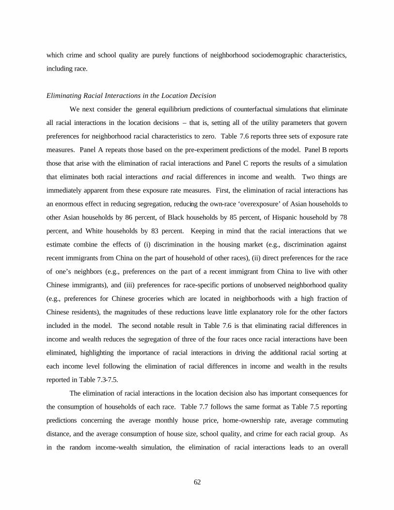
62
which crime and school quality are purely functions of neighborhood sociodemographic characteristics,
including race.
Eliminating Racial Interactions in the Location Decision
We next consider the general equilibrium predictions of counterfactual simulations that eliminate
all racial interactions in the location decisions – that is, setting all of the utility parameters that govern
preferences for neighborhood racial characteristics to zero. Table 7.6 reports three sets of exposure rate
measures. Panel A repeats those based on the pre-experiment predictions of the model. Panel B reports
those that arise with the elimination of racial interactions and Panel C reports the results of a simulation
that eliminates both racial interactions and racial differences in income and wealth. Two things are
immediately apparent from these exposure rate measures. First, the elimination of racial interactions has
an enormous effect in reducing segregation, reducing the own-race ‘overexposure’ of Asian households to
other Asian households by 86 percent, of Black households by 85 percent, of Hispanic household by 78
percent, and White households by 83 percent. Keeping in mind that the racial interactions that we
estimate combine the effects of (i) discrimination in the housing market (e.g., discrimination against
recent immigrants from China on the part of household of other races), (ii) direct preferences for the race
of one’s neighbors (e.g., preferences on the part of a recent immigrant from China to live with other
Chinese immigrants), and (iii) preferences for race-specific portions of unobserved neighborhood quality
(e.g., preferences for Chinese groceries which are located in neighborhoods with a high fraction of
Chinese residents), the magnitudes of these reductions leave little explanatory role for the other factors
included in the model. The second notable result in Table 7.6 is that eliminating racial differences in
income and wealth reduces the segregation of three of the four races once racial interactions have been
eliminated, highlighting the importance of racial interactions in driving the additional racial sorting at
each income level following the elimination of racial differences in income and wealth in the results
reported in Table 7.3-7.5.
The elimination of racial interactions in the location decision also has important consequences for
the consumption of households of each race. Table 7.7 follows the same format as Table 7.5 reporting
predictions concerning the average monthly house price, home-ownership rate, average commuting
distance, and the average consumption of house size, school quality, and crime for each racial group. As
in the random income-wealth simulation, the elimination of racial interactions leads to an overall
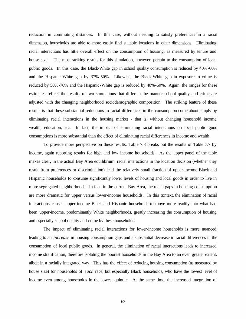
63
reduction in commuting distances. In this case, without needing to satisfy preferences in a racial
dimension, households are able to more easily find suitable locations in other dimensions. Eliminating
racial interactions has little overall effect on the consumption of housing, as measured by tenure and
house size. The most striking results for this simulation, however, pertain to the consumption of local
public goods. In this case, the Black-White gap in school quality consumption is reduced by 40%-60%
and the Hispanic-White gap by 37%-50%. Likewise, the Black-White gap in exposure to crime is
reduced by 50%-70% and the Hispanic-White gap is reduced by 40%-60%. Again, the ranges for these
estimates reflect the results of two simulations that differ in the manner school quality and crime are
adjusted with the changing neighborhood sociodemographic composition. The striking feature of these
results is that these substantial reductions in racial differences in the consumption come about simply by
eliminating racial interactions in the housing market - that is, without changing household income,
wealth, education, etc. In fact, the impact of eliminating racial interactions on local public good
consumptions is more substantial than the effect of eliminating racial differences in income and wealth!
To provide more perspective on these results, Table 7.8 breaks out the results of Table 7.7 by
income, again reporting results for high and low income households. As the upper panel of the table
makes clear, in the actual Bay Area equilibrium, racial interactions in the location decision (whether they
result from preferences or discrimination) lead the relatively small fraction of upper-income Black and
Hispanic households to consume significantly lower levels of housing and local goods in order to live in
more segregated neighborhoods. In fact, in the current Bay Area, the racial gaps in housing consumption
are more dramatic for upper versus lower-income households. In this context, the elimination of racial
interactions causes upper-income Black and Hispanic households to move more readily into what had
been upper-income, predominantly White neighborhoods, greatly increasing the consumption of housing
and especially school quality and crime by these households.
The impact of eliminating racial interactions for lower-income households is more nuanced,
leading to an increase in housing consumption gaps and a substantial decrease in racial differences in the
consumption of local public goods. In general, the elimination of racial interactions leads to increased
income stratification, therefore isolating the poorest households in the Bay Area to an even greater extent,
albeit in a racially integrated way. This has the effect of reducing housing consumption (as measured by
house size) for households of each race, but especially Black households, who have the lowest level of
income even among households in the lowest quintile. At the same time, the increased integration of

64
households dramatically reduces the substantial gaps in the consumption of local public goods that are
present in the current Bay Area equilibrium.
Geography
One final table helps to illustrate the importance of racial interactions in the housing market.
Table 7.9 reports the results of two simulations: the first eliminates racial differences in job locations
among working households, while the second eliminates racial differences in job locations and increases
the disutility of commuting ten-fold. To eliminate racial differences in job locations, we simply assign
each working household a new job location drawn at random from the distribution of employment in the
Bay Area. Importantly, this experiment only changes the geography of the location decision, not a
household’s income. As the top panel of Table 7.9 illustrates, eliminating racial differences in job
locations actually leads to an increase in the segregation of each race in equilibrium! This result is
especially striking because one might have thought the geographic distribution of employment is also
racially concentrated with the Bay Area. As it turns out, however, randomly distributing the job locations
of households of each race throughout the Bay Area leads to a substantial increase in segregation. This
result occurs because the current racial distribution of employment in the Bay Area leaves many sub-
regions of the Bay Area with a limited number of Asian, Black, or Hispanic households. In these sub-
regions, households of these racial groups have little choice but to live in neighborhoods with relatively
few households of the same race. With a more even spatial distribution of jobs, however, racially
segregated neighborhoods form throughout the metropolitan area, significantly increasing the overall
level of racial sorting.66
8 CONCLUSION
This paper makes two related contributions to the literature. First, it develops a new framework
for analyzing the sorting of households across the neighborhoods of a large metropolitan area, taking
equilibrium considerations explicitly into account. The framework’s discrete choice model enables
66 The lower panel of Table 7.9 reports results for an analogous experiment that also increases the disutility of commuting ten-fold. In this case, the segregation of households of each race is reduced as households put more weight on locations nearer their place-of-work. This additional simulation illustrates an important point, namely that the results of the job randomization simulation are highly dependent on the strength of the estimated racial interactions relative to the disutility of commuting. In the limit, as the disutility of commuting goes to –, the randomization of job locations across race would lead to perfect integration.

65
household preferences to be specified in a very flexible way, preferences that vary with a wide range of
house, neighborhood, and household characteristics. Among the choice characteristics, we allow
household utility to depend on choice-specific unobservables – unobservable, that is, to the
econometrician – forcing us to confront an important endogeneity problem: house prices and
neighborhood compositions, over which households have preferences, will be correlated with unobserved
housing and neighborhood quality. To identify preferences in the face of this, we provide a general
instrumental variables strategy and demonstrate that instruments arise naturally out of the logic of the
housing market equilibrium. Using an extremely rich dataset based on restricted access Census micro-
data, the resulting parameter estimates provide the most comprehensive view in the literature to date of
household preferences over housing and neighborhood characteristics, and of the heterogeneity in these
preferences. In general, this framework can be readily applied to answering a variety of economic and
policy questions in urban economics, local public finance, and the economics of education where a
consideration of the housing market equilibrium and the non-random sorting of households across
locations play an important role.
The second main contribution of the paper is to use these estimated parameters along with the
equilibrium model of sorting to explore a series of issues related to segregation in the housing market.
Despite controlling for the likely correlation of neighborhood racial composition and unobserved housing
and neighborhood quality, we estimate strong segregating racia l interactions in the location decision, and
while it is not possible to distinguish whether these preferences are a manifestation of discrimination or
strong tastes for self-segregation, it is very clear that racial factors play a significant role in the residential
location decision of many households. Using the estimated preferences, we then conduct a series of
general equilibrium counterfactual simulations designed to shed new light on the causes and
consequences of residential segregation.
A number of the findings from our general equilibrium analysis are striking. First, removing
racial differences in income and wealth or education leads to a marked increase in the segregation of each
race. Here, it is noteworthy that partial equilibrium calculations using the model estimates produce the
opposite conclusion, failing to account for the compounding effects of adjustments in neighborhood
socio-demographics. The key insight that the general equilibrium approach affords is that given the
combination of strong, segregating racial interactions and the relatively small fractions of Asian, Black,
and Hispanic households in the Bay Area, the elimination of racial differences in income/wealth (or,

66
education) spreads households in these racial groups much more evenly across the income distribution,
causing more racial sorting to occur at all points in the distribution – e.g., leading to the formation of
wealthy, segregated Black and Hispanic neighborhoods. Moreover, contrary to research that points to the
geographic distribution of employment as an important segregating force (e.g., Bajari and Kahn (2001)),
we find that randomizing job locations throughout the Bay Area would in fact lead to increases in
segregation. As the finding indicates, the current employment distribution combined with the cost of
commuting tends to lead different types of household to live together; spreading jobs out would permit
greater segregation, in line with self-segregating preferences. It is worth emphasizing that this result
again is due in no small part to the relatively small fraction of Asian, Black, and Hispanic households in
the Bay Area.
Eliminating the portion of the preference structure relating to preferences for neighborhood race
almost entirely eliminates segregation on the basis of race, leaving little explanatory role for factors
related to the other features included in our analysis. The elimination of racial interactions also provides
clear evidence that certain household types under-consume housing and school quality in order to live in
communities with the racial composition that they prefer. For example, we find that upper income Black
and Hispanic households would consume significantly more school quality in the absence of any
preferences for neighborhood race. This finding has important implications for policy. It indicates that
decoupling housing choice from public school assignment could lead to improvements in education
quality for a significant subset of minority households, with all the associated benefits that would bring.

67
References Anas, Alex, (1982), Residential Location Markets and Urban Transportation: Economic Theory, Econometrics and Public Policy Analysis, Academic Press, New York. Anas, Alex, and Chausie Chu, (1984), “Discrete Choice Models and the Housing Price and Travel to Work Elasticities of Location Demand,” Journal of Urban Economics, Vol 15, pp. 107-123. Bajari, Patrick and Lanier Benkhard, (2002), “Demand Estimation with Heterogeneous Consumers and Unobserved Product Characteris tics: A Hedonic Approach,” unpublished manuscript, Stanford University. Bajari, Patrick, and Matthew Kahn (2001), “Why Do Blacks Live in Cities and Whites Live in Suburbs?” unpublished manuscript, Stanford University. Bartik, Timothy, (1987), “The Estimation of Demand Parameters in Hedonic Price Models,” Journal of Political Economy , 95:81-88. Bayer, Patrick, (1999), “Essays Aimed at Understanding Observed Differences in the Consumption of School Quality,” Stanford University Dissertation. Bayer, Patrick, Robert McMillan, and Kim Rueben, (2002), “What Drives Racial Segregation? Evidence from the San Francisco Bay Area Using Micro-Census Data,” unpublished manuscript, Yale University. Bayer, Patrick, Robert McMillan, and Kim Rueben, (2002b), “Using Choice and Price Variation to Understand the Nature of Racial Preferences,” work in progress. Bayer, Patrick and Christopher Timmins, (2002), “The Identification of Social Interactions in Endogenous Sorting Models,” unpublished manuscript, Yale University. Benabou, Roland, (1993), “The Workings of a City: Location, Education, and Production,” Quarterly Journal of Economics, 108(3), pp.619-652. Benabou, Roland, (1996), “Heterogeneity, Stratification, and Growth: Macroeconomic Implications of Community Structure and School Finance,” American Economic Review, Vol. 86, No. 3., pp. 584-609. Berry, Steven, (1994), “Estimating Discrete-Choice Models of Product Differentiation,” RAND Journal of Economics, Vol. 25, pp. 242-262. Berry, Steven, James Levinsohn, and Ariel Pakes, (1995), “Automobile Prices in Market Equilibrium,” Econometrica, Vol 63, pp. 841-890. Berry, Steven, Oliver Linton, and Ariel Pakes, (2002), “Limit Theorems for Estimating the Parameters of Differentiated Product Demand Systems,” unpublished manuscript, Yale University. Borjas, George J., (1995), “Ethnicity, Neighborhoods, and Human-Capital Externalities,” American Economic Review, 85(3): 365-390. Borjas, George J., (1998), “To Ghetto or Not to Ghetto: Ethnicity and Residential Segregation.” Journal of Urban Economics, 44: 228-253 Brown, James and Harvey Rosen (1982), “On the Estimation of Structural Hedonic Price Models,” Econometrica, 50: 765-9. Cutler, David and Edward Glaeser, (1997), “Are Ghettos Good or Bad?” Quarterly Journal of Economics, August: 826-72.

68
Cutler, David, Edward Glaeser, and Jacob Vigdor, (1999), “The Rise and Decline of the American Ghetto.” Journal of Political Economy , 107(3): 455-506. Duncombe, William, Mark Robbins, and Douglas Wolf, (1999), “Retire to Where? A Discrete Choice Model of Residential Location,” unpublished manuscript, Syracuse University. Ekeland, Ivar, James Heckman, and Lars Nesheim, (2002), “Identification and Estimation of Hedonic Models,” unpublished manuscript, University of Chicago. Epple, Dennis, (1987), “Hedonic Prices and Implicit Markets: Estimating Demand and Supply Functions for Differentiated Products,” Journal of Political Economy , 107: 645-81. Epple, D., R. Filimon, and T. Romer, (1984), “Equilibrium Among Local Jurisdictions: Towards an Integrated Approach of Voting and Residential Choice,” Journal of Public Economics, Vol. 24, pp. 281-304. Epple, D., R. Filimon, and T. Romer, (1993), “Existence of Voting and Housing Equilibrium in a System of Communities with Property Taxes,” Regional Science and Urban Economics, Vol. 23, pp. 585-610. Epple, Dennis and Holger Sieg, (1999), “Estimating Equilibrium Models of Local Jurisdictions,” Journal of Political Economy , Vol. 107, No. 4., pp. 645-681. Fernandez, Raquel and Richard Rogerson, (1996), “Income Distribution, Communities, and the Quality of Public Education.” Quarterly Journal of Economics, Vol. 111, No. 1., pp. 135-164. Gabriel, S. and S. Rosenthal, (1989), “Household Location and Race: Estimates of a Multinomial Logit Model,” Review of Economics and Statistics, 71: 240-9. Harsman, Bjorn and John M. Quigley, (1995) “The Spatial Segregation of Ethnic and Demographic Groups: Comparative Evidence from Stockholm and San Francisco,” Journal of Urban Economics, 37: 1-16. Massey, Douglas S., and Nancy A. Denton, (1987), “Trends in the Residential Segregation of Blacks, Hispanics, and Asians,” American Sociological Review, 52: 802-825. Massey, Douglas S., and Nancy A. Denton, (1989), “Hypersegregation in United States Metropolitan Areas – Black and Hispanic Segregation along Five Dimensions,” Demography, 26: 373-91. Massey, Douglas S., and Nancy A. Denton, (1993), American Apartheid: Segregation and the Making of the Underclass. Cambridge, MA: Harvard University Press. McFadden, Daniel, (1973), “Conditional Logit Analysis of Qualitative Choice Behavior,” in P. Zarembka, eds., Frontiers of Econometrics, Academic Press, New York. McFadden, Daniel, (1978), “Modeling the Choice of Residential Location,” in eds. Karlquist, A., et al., Spatial Interaction Theory and Planning Models, Elsevier North-Holland, New York. Miller, V. and John M. Quigley, (1990), “Segregation by Racial and demographic Group: Evidence from the San Francisco Bay Area,” Urban Studies, 27: 3-21. Nechyba, Thomas J., (1997), “Existence of Equilibrium and Stratification in Local and Hierarchical Tiebout Economies with Property Taxes and Voting,” Economic Theory, Vol. 10, pp. 277-304. Nechyba, Thomas J., (1999), “School Finance Induced Migration and Stratification Patterns: the Impact of Private School Vouchers,” Journal of Public Economic Theory, Vol. 1. Nechyba, Thomas J., and Robert P. Strauss, (1998), “Community Choice and Local Public Services: A Discrete Choice Approach,” Regional Science and Urban Economics, Vol. 28, pp. 51-73.

69
Quigley, John M., (1985), “Consumer Choice of Dwelling, Neighborhood, and Public Services,” Regional Science and Urban Economics, Vol. 15(1). Rosen, Sherwin, (1974), “Hedonic Prices and Implicit Markets: Product Differentiation in Pure Competition,” Journal of Political Economy , 82: 34-55. Schelling, Thomas C., (1969), “Models of Segregation.” American Economic Review, 59(2): 488-93. Schelling, Thomas C., (1971), “Dynamic Models of Segregation,” Journal of Mathematical Sociology, 1: 143-186 . Schelling, Thomas C., (1978), Micromotives and Macrobehavior, Norton: New York. Tiebout, Charles M., (1956), “A Pure Theory of Local Expenditures,” Journal of Political Economy , 64: 416-424. Figure 7.1: Segregation Patterns in the Bay Area

70
Technical Appendix Proof of Proposition 2.1:67 Following the assumptions of Proposition 2.1, consider a utility specification that is a linear, decreasing function of ph:
(A.1) ihh
ip
ih
ihh
iphh
iih
ih pWpXZWV εαεαξ +−=+−= ),,(
If εε is drawn from a continuous distribution, the probability Pi
h that household i chooses house h as:
(A.2) )p,X,,( ξξih
ih ZfP =
is continuous and differentiable in p with derivatives that obey the following strict inequalities: 0<∂∂ hih pP and
hkpP kih ≠>∂∂ ,0 , if -αp
i is negative for each household i. Aggregating these probabilities over all households
yields the predicted number of households that choose each house h, hN :
(A.3) ∑•=i
ihh PN µˆ
Given the properties of Phi just described, hN is also continuous and differentiable in p with derivatives that obey
the following strict inequalities: 0ˆ <∂∂ hh pN and hkpN kh ≠>∂∂ ,0ˆ . In order for the housing market to clear,
the number of households choosing each house h must equal the measure of the continuum of houses that each observed house represents:
(A.4) hNh ∀= ,ˆ µ
Also note that for any finite values of , hkpk ≠ , hN approaches arbitrarily close to zero as ph goes to +, while
hN approach arbitrarily close to µN as ph approaches –. Holding the price of one house fixed (without loss of generality set p0 = 0), we will show that a unique
vector of prices clears the market, i.e., that a unique vector )(ˆp µµ1−= N exists. We begin by defining the element-
by-element inverse )ˆ(p, hh Nr . This function is defined as the price of house h such that the predicted value hN
exactly equals µ. That is, r is implicitly defined as:
(A.5) hpNrppN Hhhh ∀= µ)),...,ˆ(p,,...,,(ˆ21
Given the properties of the function hN defined in (A.3), this element-by-element inverse exists and is continuous
and differentiable in p. Note that rh is strictly increasing in pk and does not depend on ph. Also define the vector values r = (r1, …, rN). The element-by-element inverse allows us to transform the problem of solving for the vector inverse into a
fixed-point problem, for a vector p satisfies equation (A.4) if and only if p = )Nr(p, . The method of proof is to use
a slight variant of Brouwer’s fixed-point theorem to prove existence of a fixed point of the element-by-element inverse. It is then necessary to show that there cannot be two such fixed points.
To establish existence, first hold p0 = 0 and note that )ˆ(p, hh Nr has an upper bound. This upper bound is
)ˆ,(p' hh Nr with p' set equal to any vector in RN+1 such that pk = + for )0,(hk ≠ . Define p as the largest values
67 This proof follows directly the structure of the proof that appears in the technical appendix of Berry (1994). We simply modify it here for our problem.

71
across houses of these upper bounds. There is no lower bound for ph, but the following lemma allows one to establish existence in the absence of a lower bound. Lemma. There is a value p , with the property that if one element of p, say ph, is lower than p , then there is a house
k such that )N(p,kr > pk.
Proof of Lemma. To construct p , again set pk = +, )0,(hk ≠∀ . Then define
hp as the value of ph that sets
µ=0N . Define p as any value lower than the minimum of the h
p . Now, if for the vector p there is an element h
such that ph < p , then µ>(p)ˆ0N , which implies µ•−<∑ =
)((p)ˆ 11
NNN
h h , so there is at least one element k with
µ<(p)ˆkN . For this k , )N(p,kr > pk. Q.E.D.
Now define a new function that is a truncated version of rh: ),N(p,)N(p,~ prr hh max = . Clearly )N(p,r~ is a
continuous function which maps [ p , p ]N into itself, so by Brouwer’s fixed–point theorem, )N(p,r~ has a fixed
point, p*. By the definition of p and p , p* cannot have a value at the lower bound, so p* is in the interior of
[ p , p ]N. This implies that p* is also a fixed point of the unrestricted function )Nr(p, , which establishes existence.
A well-known sufficient condition for uniqueness is ∑ <∂∂k kh pr 1/ , which establishes that r is a
contraction mapping. By the implicit function theorem, ]/ˆ/[]/ˆ[/ hhkhkh pNpNpr ∂∂∂∂−=∂∂ . From this
∑ <∂∂k kh pr 1/ if and only if the following dominant diagonal condition holds:
(A.6) hhhk
kh pNpN ∂∂<∂∂∑≠
/ˆ/ˆ),( 0
To establish this condition, note that increasing all prices (including p0) by the same amount will not change the demand for any house. Then (A.6) follows from:
./ˆ/ˆ/ˆ/ˆ/ˆ/ˆ),(
hhhhhhk
khhhhk
kh pNpNpNpNpNpN ∂∂<∂∂+∂∂−=∂∂⇒=∂∂−∂∂ ∑∑≠≠
00
0
Q.E.D. Proof of Lemma 2.1 . Lemma 2.1 follows directly if we can show that the mapping that defines the fixed-point problem above is continuous in x, as the unique fixed-point p* of a mapping continuous in both x and p is also continuous in x. The assumption that utility is continuous in xh along with assumption about the continuous
distribution of εε implies that Phi is continuous in x for all i, which in turn implies that hN is continuous in x, which
in turn implies that the element-by-element inverse defined in (A.5) is continuous in x. Q.E.D. Proof of Proposition 2.2. Conditional on any vector g and the primitives of the model Z, X, ξξ, Proposition 2.1 implies that a unique set of housing prices clears the market and assumption (i) ensures that this vector of market-clearing prices is continuous in g. Assumptions (ii) and (iii) in turn imply that that equation (2.11), along with the definition of the function g, implicitly defines g and represents a continuous mapping of a closed interval into itself. The existence of fixed point of this mapping, g*, follows directly from Brouwer’s fixed-point theorem. Any fixed point, g*, is associated with a unique vector of market clearing prices p* and a unique set of choice probabilities
ihP * that together satisfy the conditions for a sorting equilibrium. Consequently, the existence of a fixed point, g*,
implies the existence of a sorting equilibrium. Q.E.D.

Table 5.1: First-Stage Price Regressions
First-Stage Price RegressionsDependent Variable Monthly house price Monthly house price Monthly house priceObservations 200,000 200,000 200,000Includes full set of standard variables Shown below No Yes
Coefficient Standard Error Coefficient Standard Error Coefficient Standard Error
'Quasi-' Optimal InstrumentsPrice (/1000) 385.99 3.69 378.62 3.68Percent Black -43.7 2.03 -25.85 2.33Percent Hispanic -14.13 1.83 6.95 1.99Percent Asian 6.3 2.12 30.50 2.36Percent College Degree or More 55.96 2.62 41.36 2.83Average Neighborhood Income 274.72 2.75 269.14 2.79
Standard VariablesOwner-Occupied 201.09 4.51Number of Rooms 198.87 1.16Builts 1980s 271.45 8.77Built 1960-79 15.30 5.28Pollution Index -0.82 0.59Population Density -120.95 6.00Elevation 0.64 0.01Distance to Bay -4.65 0.45Distance to Ocean -14.12 0.31Avg Min Jan Temp -15.18 1.37Employment Accessibility Index 156.30 10.500.00Industrial land use within 1 mile -351.43 25.20percentage 1-3 miles -43.69 28.47
3-5 miles 221.33 26.290.00Commercial land use within 1 mile -354.97 18.30percentage 1-3 miles 431.65 43.40
3-5 miles 273.37 41.720.00Open space within 1 mile 83.16 13.67percentage 1-3 miles -60.80 14.32
3-5 miles -28.18 14.370.00Other urban land use within 1 mile 25.46 31.79percentage 1-3 miles 513.04 68.58
3-5 miles -278.64 55.630.00Owner-occupied, large sing-fam homes within 1 mile 120.70 2.55number with 7 or more rooms (/100) 1-3 miles 6.08 0.74
3-5 miles 7.33 0.590.00Owner-occupied, small sing-fam homes within 1 mile -37.77 2.40number with 6 or fewer rooms (/100) 1-3 miles -6.89 0.82
3-5 miles -6.64 0.660.00Owner-occupied, non-sing-fam homes within 1 mile -77.07 3.58number (/100) 1-3 miles 0.42 1.43
3-5 miles 28.98 1.280.00Renter-occupied, sing-fam homes within 1 mile -101.30 6.13number (/100) 1-3 miles 6.04 2.26
3-5 miles 10.05 1.640.00Renter-occupied, in small apart building within 1 mile 15.43 1.58number (/100) 1-3 miles -10.42 0.70
3-5 miles -8.25 0.460.00Renter-occupied, in large apart building within 1 mile 5.08 1.15number (/100) 1-3 miles 1.47 0.67
3-5 miles -0.90 0.46
F-Tests for joint significance F-stat P-value F-stat P-value F-stat P-valueStandard variables -- Variables in 3-5 mile ring 181.98 0.000'Quasi-' optimal instruments 6843.67 0.000 5096.50 0.000Variables in 3-5 mile ring and 'quasi-' optimal instruments 1295.73 0.000
Note: In the subsequent analysis, standard instruments refer to the set of land use and neighborhood housing stock variables in the 3-5 mile ring. In all subsequent analysis, the land use and neighborhood housing stock variables within 1 mile and in the 1-3 mile ring are included in the utility function. The 'quasi-' optimal instruments are based on the predicted vector of market-clearing house prices and neighborhood sociodemographic characteristics using only the exogenous components of the sorting model -- full details are provided in Section 5 of the text.
72

Table 6.1: Interaction Parameter Estimates
House Characteristics Neighborhood Sociodemographic Composition Other Neighborhood Attributes Access to Work
Monthly Owner- Number Built in Built in % % % % College Average Average Pollution Population Distance Distance Crime Avg Min Distance Dist-Work EmploymentHouse PriceOccupied Rooms 1980s 1960-1979 Black Hispanic Asian Degree or Income Math Score Index Elevation Density to Bay to Ocean Index Temp To Work Squared Access Index
(/1000) More (/10000) (/100) (/100) (/100) (/1000)
Hhld Income 0.120 0.328 0.050 0.274 0.093 -0.122 -0.315 0.064 0.351 0.011 0.023 -0.007 0.002 -0.069 0.005 0.004 -0.004 0.025 0.002 -0.011 0.033(/10,000) (0.005) (0.02) (0.001) (0.047) (0.035) (0.035) (0.256) (0.047) (0.025) (0.002) (0.012) (0.001) (0.004) (0.009) (0.001) (0.001) (0.001) (0.003) (0.) (0.001) (0.014)
Captital Income 0.054 0.309 0.009 -0.089 0.031 -1.249 -0.064 -1.002 0.303 -0.015 0.151 0.020 -0.001 0.010 -0.016 -0.028 -0.007 -0.044 -0.027 0.006 0.021(/10,000) (0.017) (0.032) (0.012) (0.054) (0.356) (0.064) (0.122) (0.087) (0.058) (0.003) (0.003) (0.002) (0.022) (0.02) (0.002) (0.001) (0.001) (0.005) (0.001) (0.001) (0.006)
Black 0.129 -1.135 0.045 0.068 0.685 16.376 7.073 7.435 2.753 0.013 -1.350 0.025 0.047 -0.859 -0.071 0.047 0.030 0.020 -0.048 0.055 0.015(0.182) (0.192) (0.106) (0.58) (0.239) (0.522) (5.422) (0.932) (0.593) (0.037) (0.202) (0.026) (0.066) (0.16) (0.015) (0.012) (0.009) (0.043) (0.006) (0.006) (0.272)
Hispanic 0.198 -0.010 -0.434 0.011 -0.240 4.242 9.571 2.658 1.924 0.039 0.007 0.022 -0.088 0.239 0.008 0.033 0.011 0.004 0.063 -0.173 -0.134(0.125) (0.244) (0.068) (0.733) (0.184) (0.685) (0.888) (0.463) (0.335) (0.028) (0.276) (0.027) (0.208) (0.142) (0.002) (0.008) (0.032) (0.068) (0.005) (0.014) (0.04)
Asian 0.593 1.897 -0.807 1.198 0.621 3.852 1.611 17.974 0.956 -0.020 -0.366 0.015 -0.060 -0.118 0.022 -0.004 -0.001 -0.043 0.002 0.013 -0.022(0.129) (0.287) (0.213) (1.173) (0.176) (0.426) (0.62) (0.641) (0.475) (0.026) (0.246) (0.025) (0.051) (0.211) (0.016) (0.009) (0.012) (0.056) (0.006) (0.008) (0.037)
Some College 0.487 -0.130 0.081 -0.004 -1.516 0.171 1.934 0.963 0.093 -0.005 -0.004 0.008 -0.014(0.205) (0.314) (0.105) (0.406) (0.549) (0.633) (0.401) (0.114) (0.142) (0.025) (0.005) (0.009) (0.003)
College Degree 0.491 0.287 0.068 2.112 -0.771 -0.951 8.219 0.558 0.461 0.015 0.012 0.001 0.093(0.139) (0.113) (0.069) (0.413) (0.367) (0.587) (0.429) (0.159) (0.097) (0.006) (0.002) (0.009) (0.02)
Working 0.286 0.723 0.017 -1.549 -0.870 -1.309 -1.281 -0.429 0.413 -0.222(0.083) (0.554) (0.056) (0.481) (0.402) (0.469) (0.292) (0.001) (0.004) (0.022)
Age 0.010 0.096 0.005 -0.003 -0.100 0.018 -0.023 0.013 -0.003 0.001 0.000(0.002) (0.007) (0.002) (0.009) (0.016) (0.051) (0.035) (0.005) (0.001) (0.) (0.001)
# Persons in Hhld 0.214 -0.289 0.324 -0.763 -0.262 1.231 2.229 1.035 -1.163 0.223 0.060 -0.009 0.017 -0.032(0.035) (0.189) (0.013) (0.103) (0.034) (0.152) (0.129) (0.203) (0.178) (0.039) (0.036) (0.002) (0.005) (0.009)
# of Kids in Hhld -0.224 0.157 -0.030 0.862 0.445 -0.871 -1.600 -0.070 -0.158 -0.011 -0.311 0.002 0.018 -0.040 -0.057(0.035) (0.047) (0.049) (1.054) (0.05) (0.226) (0.192) (0.94) (0.586) (0.062) (0.055) (0.002) (0.002) (0.005) (0.015)
Income x Black -0.330(0.15)
Income x Hispanic 0.701(0.138)
Income x Asian -0.154(0.096)
College Degree x Black -4.037(1.313)
College Degree x Hispanic -0.786(1.463)
College Degree x Asian -3.206(0.828)
Note: The parameters shown describe the elements of the utility function that interact household characteristics, shown in row headings, with choice characteristics, shown in column headings. Standard errors in parentheses. Bold-face indicates statistical significance at 95 percent level.
73

Table 6.2: Implied Mean Marginal Willingness-to-Pay (MWTP) Measures
Implied Mean MWTP Measures Hedonic Price RegressionRegression Method OLS IV IV OLS
Dependent Variable in Underlying Regression Choice-specific constant Choice-specific constant Choice-specific constant House Price
Endogenous Variables in Underlying Regression None Price Price, N'hood sociodemogs. None
Instruments 'Quasi-' Optimal 'Quasi-' Optimal
Observations 200,000 200,000 200,000 200,000
Implied coefficient -1.90 -0.15 -0.15 0.00on choice-specific constant (0.02) (0.01) (0.01) (---)
Percent Black -6305.62 -605.58 -590.52 -144.02(54.47) (11.52) (13.38) (11.01)
Percent Hispanic -4654.13 -59.13 -30.95 364.00(84.07) (18.01) (24.43) (16.41)
Percent Asian -2266.60 -155.90 -186.22 76.70(6.44) (13.34) (15.86) (12.59)
Percent College Degree + -711.41 574.01 660.81 668.48(55.93) (13.09) (17.59) (10.84)
Average Income -20.96 3.96 3.58 13.54(/10,000) (2.68) (0.55) (0.55) (3.22)
Crime Rate -31.70 -1.18 -1.10 0.27(1.03) (0.23) (0.23) (0.22)
Average Math Score -8.85 0.85 0.73 1.76(0.03) (0.06) (0.06) (0.05)
Owner-Occupied 866.76 208.82 208.95 149.97(16.76) (3.67) (4.07) (3.25)
Number of Rooms 46.83 132.59 132.21 140.77(4.57) (1.57) (2.07) (0.83)
Built in 1980s 439.58 174.71 171.11 103.71(32.90) (6.88) (4.61) (4.27)
Built in 1960s, 1970s 247.16 25.84 25.63 11.70(19.49) (4.00) (3.14) (3.09)
Pollution Index -15.16 -2.89 -3.02 -1.35(1.98) (0.42) (0.41) (0.41)
Population Density -231.62 -56.87 -49.09 -43.21(22.86) (4.69) (4.68) (4.46)
Elevation -111.64 14.43 13.12 20.45(in 100 foot units) (4.78) (1.06) (1.07) (0.91)
Distance to Bay 27.96 0.39 0.42 -0.04(1.38) (0.31) (0.31) (0.27)
Distance to Ocean 24.11 -3.62 -3.30 -6.58(1.10) (0.24) (0.24) (0.22)
Avg. Min. Jan. Temperature 48.58 -0.88 -0.40 -6.50(4.60) (0.99) (0.95) (0.90)
Employment Access -54.83 -4.46 -4.44 3.13(3.61) (0.29) (0.29) (0.35)
Distance to Work -598.33 -48.67 -48.43(4.08) (0.33) (0.33)
Distance to Work - Squared 576.50 46.90 46.66(6.05) (0.49) (0.49)
Includes variables describingland use and housing stock Yes Yes Yes Yeswithin 1 mile, and 1-3 mile ring
Note: The first three columns of the table report the mean marginal willingness-to-pay (MWTP) measures implied by three different estimates of the choice-specific constant regression (equation 4.2). The regressions underlying these mean MWTP measures are shown in columns 1, 4, and 5 in Appendix Table 2.The first column reports the estimates that result when the choice-specific constant regression is estimated via OLS; the middle two columns report IV estimatesthat use the 'quasi-' optimal instruments, instrumenting for price, and price and neighborhood sociodemographic variables respectively. The final columnreturns the estimate of a standard hedonic price regression. Standard errors in parentheses. Bold-face indicates statistical significance at 95 percent level.
74

Table 6.3: Heterogeneity in Marginal Willingness-to-Pay Measures
Owner Number Built Built % Black % Hisp % Asian % College Average Average Pollution Population Crime DistanceOccupied Rooms 1980s 60s-70s vs. White vs. White vs. White Degree Income Math Score Index Elevation Density Index To Work
Change Reported: vs. Rental +1 room vs. pre-60s vs. pre-60s +10% +10% +10% +10% +$10,000 +1 st.dev. +1 st.dev. +1 st.dev. +1 st.dev. +1 st.dev. +1 mile(6-7 miles)
Mean Willingness-to-Pay 209 132 114 21 -59 -3 -19 66 36 27 -13 23 -26 -13 -42
Household Income (Non-Capital sources) 40 8 32 11 -2 -4 1 5 14 1 -4 1 -4 -6 -1(+10,000)
Household Income (Capital sources) 76 9 23 14 -17 -4 -11 4 -4 7 6 1 -4 -15 -4(+10,000)
Black -127 7 9 79 187 81 85 32 18 -57 12 9 -51 38 -6vs. White
Hispanic 4 -47 4 -27 48 111 30 23 44 1 10 -17 14 14 6vs. White
Asian 245 -88 153 77 42 19 216 16 -22 -14 7 -11 -9 -3 -3vs. White
College Degree 47 16 22 -9 -13 99 26 27 27 19 -1vs. HS degree or less
Working 91 6 -20 -10 -16 -12vs. Not working
Age 111 7 -1 -11 2 -2 6 -4(+10 years)
Number of Adults -28 41 -86 -30 13 26 12 -12 10 3 -2(+1 adult)
Number of Children -16 34 7 19 5 8 11 -15 9 -14 3 3(+1 child)
Note: The first row of table reports the mean marginal willingness-to-pay (MWTP) for the change reported in the column heading. The remaining rows report the difference in willingness to pay associated with the change listed in the row heading holding all other factors equal. All measures are in terms of monthly house price. Bold-face indicates statistical significance at 95 percent level.
75
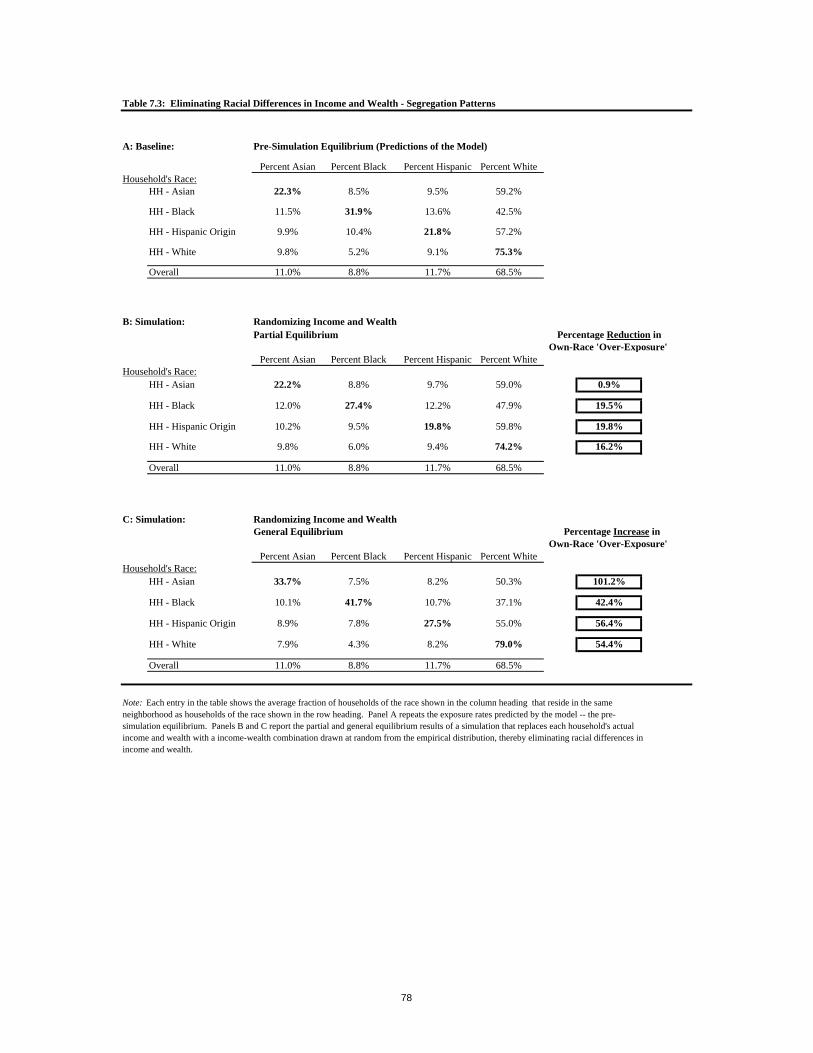
Table 7.3: Eliminating Racial Differences in Income and Wealth - Segregation Patterns
A: Baseline: Pre-Simulation Equilibrium (Predictions of the Model)
Percent Asian Percent Black Percent Hispanic Percent WhiteHousehold's Race:
HH - Asian 22.3% 8.5% 9.5% 59.2%
HH - Black 11.5% 31.9% 13.6% 42.5%
HH - Hispanic Origin 9.9% 10.4% 21.8% 57.2%
HH - White 9.8% 5.2% 9.1% 75.3%
Overall 11.0% 8.8% 11.7% 68.5%
B: Simulation: Randomizing Income and WealthPartial Equilibrium Percentage Reduction in
Own-Race 'Over-Exposure' Percent Asian Percent Black Percent Hispanic Percent White
Household's Race:HH - Asian 22.2% 8.8% 9.7% 59.0% 0.9%
HH - Black 12.0% 27.4% 12.2% 47.9% 19.5%
HH - Hispanic Origin 10.2% 9.5% 19.8% 59.8% 19.8%
HH - White 9.8% 6.0% 9.4% 74.2% 16.2%
Overall 11.0% 8.8% 11.7% 68.5%
C: Simulation: Randomizing Income and WealthGeneral Equilibrium Percentage Increase in
Own-Race 'Over-Exposure' Percent Asian Percent Black Percent Hispanic Percent White
Household's Race:HH - Asian 33.7% 7.5% 8.2% 50.3% 101.2%
HH - Black 10.1% 41.7% 10.7% 37.1% 42.4%
HH - Hispanic Origin 8.9% 7.8% 27.5% 55.0% 56.4%
HH - White 7.9% 4.3% 8.2% 79.0% 54.4%
Overall 11.0% 8.8% 11.7% 68.5%
Note: Each entry in the table shows the average fraction of households of the race shown in the column heading that reside in the same neighborhood as households of the race shown in the row heading. Panel A repeats the exposure rates predicted by the model -- the pre-simulation equilibrium. Panels B and C report the partial and general equilibrium results of a simulation that replaces each household's actualincome and wealth with a income-wealth combination drawn at random from the empirical distribution, thereby eliminating racial differences in income and wealth.
78

Table 7.2: The Distribution of Selected Household Characteristics for Households of Each Race
Variable Asian Black Hispanic White Overall
Household head (HH) is high school dropout 0.19 0.23 0.39 0.10 0.16HH graduated from high school 0.14 0.22 0.22 0.18 0.18HH has some college 0.18 0.28 0.19 0.23 0.23HH has bachelor's degree 0.33 0.20 0.16 0.32 0.29HH has advanced degree 0.16 0.06 0.05 0.17 0.14
Household income less than $12K 0.13 0.26 0.14 0.10 0.12Household income $12-20K 0.09 0.14 0.12 0.08 0.09Household income $20-35K 0.18 0.23 0.24 0.19 0.20Household income $35-50K 0.18 0.16 0.21 0.18 0.18Household income $50-75K 0.23 0.14 0.19 0.22 0.21Household income $75-100K 0.12 0.05 0.07 0.11 0.10Household receives public assistance income 0.13 0.21 0.11 0.05 0.08Household has capital income 0.48 0.17 0.25 0.56 0.48
HH over 65 0.13 0.17 0.11 0.21 0.18HH divorced 0.07 0.20 0.14 0.16 0.15Number of adults in the household 2.48 1.85 2.40 1.86 2.00Number of pre-kindergarten children in household 0.31 0.27 0.40 0.17 0.22Number of children grades K-8 in household 0.46 0.41 0.54 0.22 0.30umber of children grades 9-12 in household 0.14 0.11 0.14 0.06 0.08
Spanish spoken in household 0.01 0.04 0.68 0.03 0.10Asian language spoken in household 0.76 0.01 0.02 0.01 0.11HH not a US citizen 0.15 0.01 0.12 0.01 0.04HH a naturalized citizen 0.04 0.00 0.03 0.00 0.01HH entered the US in 1980s 0.33 0.02 0.15 0.02 0.07HH entered the US in 1970s 0.26 0.01 0.14 0.02 0.06
Number of Observations 30271 18501 26675 167897 243344
77

Table 7.1: Racial Segregation - Full Sample, Sample Used in Analysis, Model's Predictions
Average Racial Composition of Census Block Group
A: Full Sample
Percent Asian Percent Black Percent Hispanic Percent WhiteHousehold's Race:
HH - Asian 22.5% 8.3% 11.7% 57.4%
HH - Black 11.6% 40.1% 11.4% 36.9%
HH - Hispanic Origin 12.9% 9.1% 21.8% 56.2%
HH - White 10.4% 4.8% 9.3% 75.5%
Overall 12.3% 8.8% 11.2% 67.7%
B: Sample of 10,000
Percent Asian Percent Black Percent Hispanic Percent WhiteHousehold's Race:
HH - Asian 23.6% 8.0% 10.4% 58.0%
HH - Black 11.1% 41.9% 11.4% 35.6%
HH - Hispanic Origin 11.4% 9.0% 24.0% 55.6%
HH - White 10.1% 4.5% 8.8% 76.6%
Overall 11.0% 8.8% 11.7% 68.5%
C: Predictions of Model
Percent Asian Percent Black Percent Hispanic Percent WhiteHousehold's Race:
HH - Asian 22.3% 8.5% 9.5% 59.2%
HH - Black 11.5% 31.9% 13.6% 42.5%
HH - Hispanic Origin 9.9% 10.4% 21.8% 57.2%
HH - White 9.8% 5.2% 9.1% 75.3%
Overall 11.0% 8.8% 11.7% 68.5%
Note: Each entry in the table shows the average fraction of households of the race shown in the column heading that reside in the same neighborhood as households of the race shown in the row heading. Panel A reports the exposure rate measures using the full sample of 243,344 households; Panel B reports measures using the sample of 10,000 used in the first-stage of the estimation procedure; Panel C reports the same measures based on the predictions of the model.
76
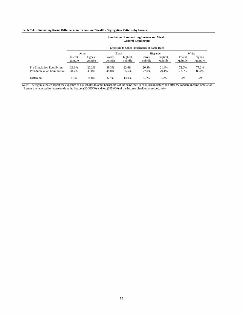
Table 7.4: Eliminating Racial Differences in Income and Wealth - Segregation Patterns by Income
Simulation: Randomizing Income and WealthGeneral Equilibrium
Exposure to Other Households of Same Race
Asian Black Hispanic Whitelowest highest lowest highest lowest highest lowest highestquintile quintile quintile quintile quintile quintile quintile quintile
Pre-Simulation Equilibrium 26.0% 20.2% 38.3% 22.6% 20.4% 21.4% 72.0% 77.2%Post-Simulation Equilibrium 34.7% 35.0% 45.0% 35.6% 27.0% 29.1% 77.0% 80.4%
Difference 8.7% 14.8% 6.7% 13.0% 6.6% 7.7% 5.0% 3.2%
Note: The figures shown report the exposure of households to other households of the same race in equilibrium before and after the random income simulation. Results are reported for households at the bottom ($0-$8500) and top ($65,000) of the income distribution respectively.
79

Table 7.5: Eliminating Racial Differences in Income and Wealth - Consumption Patterns
Simulation: Randomizing Income and WealthGeneral Equilibrium
% Reduction in % Reduction inAsian Black Hispanic White Black-White gap Black-Hisp gap
Monthly House PricePre-Simulation Equilibrium 1081.3 752.8 871.9 1115.9Post-Simulation Equilibrium - Unadjusted 1093.8 950.6 960.7 1073.6 66% 54%
Commuting Distance (miles)Pre-Simulation Equilibrium 10.70 9.86 11.42 10.80Post-Simulation Equilibrium - Unadjusted 10.06 9.84 10.91 10.24 57% -8%
Home Ownership RatePre-Simulation Equilibrium 0.624 0.368 0.418 0.605Post-Simulation Equilibrium - Unadjusted 0.612 0.480 0.500 0.580 58% 57%
House Size (rooms)Pre-Simulation Equilibrium 4.67 4.46 4.45 5.21Post-Simulation Equilibrium - Unadjusted 4.64 4.94 4.69 5.12 76% 43%
School QualityPre-Simulation Equilibrium 203.3 181.3 196.7 212.7Post-Simulation Equilibrium - Unadjusted 202.5 189.8 203.6 210.7 33% 56%Post-Simulation Equilibrium - Adjusted 202.0 181.4 201.0 212.2 2% 30%
Crime RatePre-Simulation Equilibrium 10.02 16.88 10.73 6.85Post-Simulation Equilibrium - Unadjusted 10.28 13.11 9.01 7.55 45% 62%Post-Simulation Equilibrium - Adjusted 11.44 16.90 9.82 6.76 -1% 21%
Note: This table reports the consumption of housing and local pubic goods by households of each race. Figures are reported for the pre-simulation equilibrium and the equilibrium that raises in a simulation that replaces each household's actual income and wealth witha income-wealth combination drawn at random from the empirical distribution, thereby eliminating racial differences in income and wealth.
80

Table 7.6: Eliminating Racial Interactions - Segregation Patterns
A: Baseline: Predictions of the Model
Percent Asian Percent Black Percent Hispanic Percent WhiteHousehold's Race:
HH - Asian 22.3% 8.5% 9.5% 59.2%
HH - Black 11.5% 31.9% 13.6% 42.5%
HH - Hispanic Origin 9.9% 10.4% 21.8% 57.2%
HH - White 9.8% 5.2% 9.1% 75.3%
Overall 11.0% 8.8% 11.7% 68.5%
B: Simulation: Eliminating Racial InteractionsGeneral Equilibrium Percentage Reduction in
Own-Race 'Over-Exposure' Percent Asian Percent Black Percent Hispanic Percent White
Household's Race:HH - Asian 12.5% 8.8% 10.7% 67.5% 86.4%
HH - Black 11.6% 12.3% 11.7% 63.7% 84.8%
HH - Hispanic Origin 11.4% 9.7% 14.0% 64.2% 77.7%
HH - White 11.4% 8.2% 10.2% 69.6% 83.2%
Overall 11.0% 8.8% 11.7% 68.5%
C: Simulation: Eliminating Racial Interactions and Randomizing IncomeGeneral Equilibrium Percentage Additional Reduction in
Own-Race 'Over-Exposure' with Randomized Income
Percent Asian Percent Black Percent Hispanic Percent WhiteHousehold's Race:
HH - Asian 12.1% 8.8% 11.0% 67.5% 3.8%
HH - Black 11.6% 10.8% 10.7% 66.4% 6.8%
HH - Hispanic Origin 12.4% 9.1% 15.2% 62.6% -12.0%
HH - White 11.6% 8.6% 9.7% 69.5% 1.8%
Overall 11.0% 8.8% 11.7% 68.5%
Note: Each entry in the table shows the average fraction of households of the race shown in the column heading that reside in the same neighborhood as households of the race shown in the row heading. Panel A repeats the exposure rates predicted by the model -- the pre-simulation equilibrium. Panel B reports the general equilibrium results of a simulation that eliminates the protion of household preferencesassociated with neighborhood racial composition -- that is, eliminating racial interactions in the location decision. Panel C reports the general equilibrium results of a simulation that eliminates racial interactions and randomizes income/wealth across households.
81
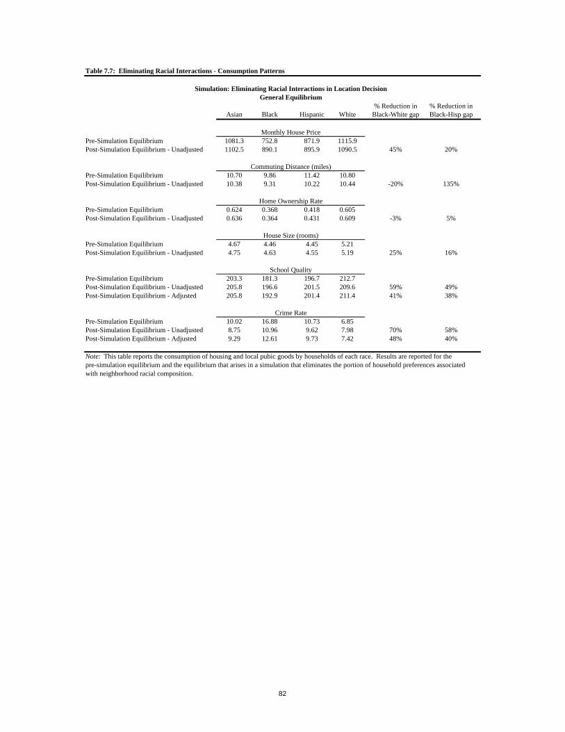
Table 7.7: Eliminating Racial Interactions - Consumption Patterns
Simulation: Eliminating Racial Interactions in Location DecisionGeneral Equilibrium
% Reduction in % Reduction inAsian Black Hispanic White Black-White gap Black-Hisp gap
Monthly House PricePre-Simulation Equilibrium 1081.3 752.8 871.9 1115.9Post-Simulation Equilibrium - Unadjusted 1102.5 890.1 895.9 1090.5 45% 20%
Commuting Distance (miles)Pre-Simulation Equilibrium 10.70 9.86 11.42 10.80Post-Simulation Equilibrium - Unadjusted 10.38 9.31 10.22 10.44 -20% 135%
Home Ownership RatePre-Simulation Equilibrium 0.624 0.368 0.418 0.605Post-Simulation Equilibrium - Unadjusted 0.636 0.364 0.431 0.609 -3% 5%
House Size (rooms)Pre-Simulation Equilibrium 4.67 4.46 4.45 5.21Post-Simulation Equilibrium - Unadjusted 4.75 4.63 4.55 5.19 25% 16%
School QualityPre-Simulation Equilibrium 203.3 181.3 196.7 212.7Post-Simulation Equilibrium - Unadjusted 205.8 196.6 201.5 209.6 59% 49%Post-Simulation Equilibrium - Adjusted 205.8 192.9 201.4 211.4 41% 38%
Crime RatePre-Simulation Equilibrium 10.02 16.88 10.73 6.85Post-Simulation Equilibrium - Unadjusted 8.75 10.96 9.62 7.98 70% 58%Post-Simulation Equilibrium - Adjusted 9.29 12.61 9.73 7.42 48% 40%
Note: This table reports the consumption of housing and local pubic goods by households of each race. Results are reported for the pre-simulation equilibrium and the equilibrium that arises in a simulation that eliminates the portion of household preferences associated with neighborhood racial composition.
82

Table 7.8: Eliminating Racial Interactions - Consumption Patterns by Income
Simulation: Eliminating Racial Interactions in Location DecisionGeneral Equilibrium
Asian Black Hispanic Whitelowest highest lowest highest lowest highest lowest highestquintile quintile quintile quintile quintile quintile quintile quintile
Home Ownership RatesPre-Equilibrium 0.391 0.785 0.253 0.548 0.209 0.628 0.397 0.758Post-Simulation - Unadjusted 0.407 0.803 0.185 0.614 0.197 0.665 0.400 0.763
House Size (rooms)Pre-Equilibrium 3.471 5.544 3.779 5.432 3.422 5.408 3.993 6.043Post-Simulation - Unadjusted 3.424 5.653 3.656 5.792 3.400 5.609 3.970 6.036
School Quality (average math score)Pre-Equilibrium 191.5 212.1 173.5 195.8 189.9 204.1 202.0 220.8Post-Simulation - Unadjusted 193.3 215.3 188.2 211.1 192.6 208.7 197.7 217.9Post-Simulation - Adjusted 191.1 214.5 184.1 210.0 193.6 209.0 198.5 220.6
Crime RatePre-Equilibrium 15.62 6.77 20.70 12.29 14.01 8.01 10.81 5.00Post-Simulation - Unadjusted 12.68 5.84 14.52 7.19 13.60 6.72 12.68 5.74Post-Simulation - Adjusted 13.79 6.26 16.33 7.85 13.63 6.64 12.51 4.88
Note: The figures shown report the consumption of housing and local public goods by households of each race in equilibrium before and after a simulation that eliminates racial interactions in the location decision. Results are reported for households at the bottom (0-$8500) and top ($65,000) of the income distribution respectively.
83
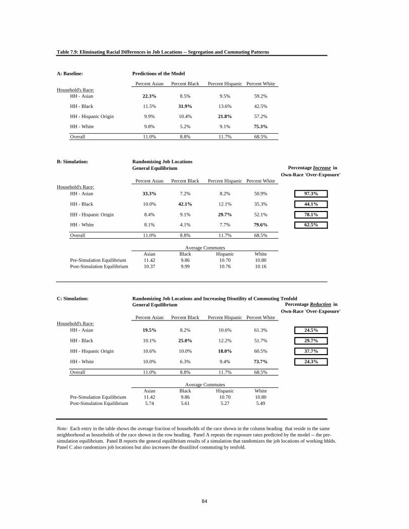
Table 7.9: Eliminating Racial Differences in Job Locations -- Segregation and Commuting Patterns
A: Baseline: Predictions of the Model
Percent Asian Percent Black Percent Hispanic Percent WhiteHousehold's Race:
HH - Asian 22.3% 8.5% 9.5% 59.2%
HH - Black 11.5% 31.9% 13.6% 42.5%
HH - Hispanic Origin 9.9% 10.4% 21.8% 57.2%
HH - White 9.8% 5.2% 9.1% 75.3%
Overall 11.0% 8.8% 11.7% 68.5%
B: Simulation: Randomizing Job LocationsGeneral Equilibrium Percentage Increase in
Own-Race 'Over-Exposure' Percent Asian Percent Black Percent Hispanic Percent White
Household's Race:HH - Asian 33.3% 7.2% 8.2% 50.9% 97.3%
HH - Black 10.0% 42.1% 12.1% 35.3% 44.1%
HH - Hispanic Origin 8.4% 9.1% 29.7% 52.1% 78.1%
HH - White 8.1% 4.1% 7.7% 79.6% 62.5%
Overall 11.0% 8.8% 11.7% 68.5%
Average CommutesAsian Black Hispanic White
Pre-Simulation Equilibrium 11.42 9.86 10.70 10.80Post-Simulation Equilibrium 10.37 9.99 10.76 10.16
C: Simulation: Randomizing Job Locations and Increasing Disutility of Commuting TenfoldGeneral Equilibrium Percentage Reduction in
Own-Race 'Over-Exposure' Percent Asian Percent Black Percent Hispanic Percent White
Household's Race:HH - Asian 19.5% 8.2% 10.6% 61.3% 24.5%
HH - Black 10.1% 25.0% 12.2% 51.7% 29.7%
HH - Hispanic Origin 10.6% 10.0% 18.0% 60.5% 37.7%
HH - White 10.0% 6.3% 9.4% 73.7% 24.3%
Overall 11.0% 8.8% 11.7% 68.5%
Average CommutesAsian Black Hispanic White
Pre-Simulation Equilibrium 11.42 9.86 10.70 10.80Post-Simulation Equilibrium 5.74 5.61 5.27 5.49
Note: Each entry in the table shows the average fraction of households of the race shown in the column heading that reside in the same neighborhood as households of the race shown in the row heading. Panel A repeats the exposure rates predicted by the model -- the pre-simulation equilibrium. Panel B reports the general equilibrium results of a simulation that randomizes the job locations of working hhlds.Panel C also randomizes job locations but also increases the disutilitof commuting by tenfold.
84

Appendix Table 1: Summary Statistics
Random Sample: 10,000* Random Sample: 200,000*
Variable Description Mean S.D. Mean S.D.
household income 53,026 52,065capital income - dividends, interest, capital gains 5,031 27,6521 if householder - Black 0.088 0.2841 if householder - Hispanic 0.110 0.3131 if householder - Asian 0.117 0.3221 if education - HS Degree or less 0.341 0.4741 if education - some college 0.222 0.4161 if education - BA Degree or more 0.437 0.4961 if someone in household working 0.688 0.464householder age (years) 47.7 16.9number of persons in household 2.61 1.57number of children under 18 in household 0.61 1.04
monthly house price 1,052 710 1,047 7321 if unit owned 0.565 0.496 0.559 0.497number of rooms 5.00 2.01 4.98 2.001 if built in 1980s 0.142 0.349 0.145 0.2351 if built in 1960s or 1970s 0.394 0.489 0.389 0.396% census block group black 0.086 0.169 0.088 0.170% census block group Hispanic 0.112 0.115 0.112 0.115% census block group Asian 0.121 0.117 0.122 0.119% census block group college degree or more 0.435 0.195 0.434 0.195average block group income 51751 29037 54900 28663average math score 207 37 207 37pollution index 24.1 4.2 24.1 4.2elevation 206 170 206 174population density 0.454 0.514 0.465 0.535distance to Bay 6.13 6.00 6.12 6.16distance to ocean 17.09 9.85 16.91 9.95crime rate 8.53 11.19 8.84 11.52avg min Jan temperature 47.2 1.9 47.6 1.9distance to work 6.11 8.32 6.12 8.28employment accessibility index 0.185 0.226 0.186 0.207
Number of owner occupied, single family homes, rooms < 7, within 1 mile 307 205Number of owner occupied, single family homes, rooms > 6, within 1 mile 173 105Number of owner occupied, non-single family homes, within 1 mile 105 169Number of renter occupied, single family homes, within 1 mile 116 72Number of renter occupied, unit in small apartment building, within 1 mile 268 423Number of renter occupied, unit in large apartment building, within 1 mile 331 711Percent land usage -- commercial, within 1 mile 0.147 0.126Percent land usage -- industrial, within 1 mile 0.039 0.087Percent land usage -- open space, within 1 mile 0.110 0.194Percent land usage -- other urban land use, within 1 mile 0.052 0.070Percent land usage -- residential, within 1 mile 0.652 0.445
Note: Summary statistics are reported for the two samples, randomly drawn from the full sample of 243,344 households used in the analysis. Due to computational constraints, the first-stage of the estimation procedure (which returns the interaction parameters and choice-specific constants) uses the sample of 10,000 and the second-stage of the estimation procedure (the choice-specific constant regressions) uses the sample of 200,000. Housing stock and land use variables are not reported for the sample of 10,000 as these variables are not used in the first-stage of the estimation, while household characteristics are not reported for the sample of 200,000 as these characteristics are not used in the second-stage of the estimation.
85

Appendix Table 2: Choice-Specific Constant Regressions
Estimates of House-Specific Constant RegressionsRegression Method OLS IV IV IV IVEndogenous Variables none House price House price House price House price
N'hood racial char. N'hood racial char.N'hood educ level N'hood educ level
Instruments Standard Standard Quasi-' Optimal Quasi-' OptimalObservations 200,000 200,000 200,000 200,000 200,000
Monthly House Price -0.525 -1.933 -2.423 -6.456 -6.488(0.006) (0.138) (0.169) (0.058) (0.059)
Percent Black -0.769 -0.775 -0.919 -0.907 -0.889(0.006) (0.008) (0.036) (0.017) (0.019)
Percent Hispanic -0.384 -0.310 0.081 -0.060 -0.032(0.007) (0.011) (0.045) (0.017) (0.025)
Percent Asian -0.193 -0.196 -0.218 -0.164 -0.196(0.001) (0.006) (0.025) (0.013) (0.017)
Percent College Degree + -0.099 0.183 -0.072 0.987 1.142(0.007) (0.026) (0.057) (0.022) (0.029)
Average Income -0.043 -0.004 -0.001 0.100 0.091(0.005) (0.007) (0.008) (0.013) (0.013)
Crime Rate -0.262 -0.207 -0.202 -0.120 -0.112(0.008) (0.011) (0.021) (0.022) (0.023)
Average Math Score -0.234 -0.132 0.036 0.276 0.238(0.001) (0.015) (0.020) (0.018) (0.018)
Owner-Occupied 0.309 0.452 0.507 0.915 0.920(0.006) (0.016) (0.019) (0.015) (0.016)
Number of Rooms 0.067 0.602 0.828 2.340 2.345(0.006) (0.053) (0.066) (0.027) (0.026)
Built in 1980s 0.074 0.129 0.204 0.362 0.356(0.005) (0.009) (0.013) (0.014) (0.014)
Built in 1960s, 1970s 0.070 0.059 0.910 0.090 0.090(0.005) (0.006) (0.008) (0.013) (0.014)
Pollution Index -0.046 -0.064 -0.034 -0.107 -0.113(0.006) (0.007) (0.008) (0.015) (0.015)
Population Density -0.089 -0.139 -0.227 -0.268 -0.233(0.008) (0.010) (0.018) (0.021) (0.022)
Elevation -0.139 -0.060 0.054 0.221 0.202(0.006) (0.011) (0.015) (0.016) (0.016)
Distance to Bay 0.123 0.099 -0.029 0.021 0.023(0.006) (0.008) (0.013) (0.016) (0.017)
Distance to Ocean 0.172 0.081 -0.070 -0.318 -0.291(0.008) (0.015) (0.020) (0.020) (0.021)
Avg. Min. Jan. Temperature 0.067 0.029 0.016 -0.015 -0.007(0.006) (0.007) (0.009) (0.016) (0.016)
Note: This table reports parameter estimates for five specifications of the choice-specific constant regression (equation 4.2). The first columnreports the estimates that result when the choice-specific constant regression is estimated via OLS; columns 2 and 3 report IV regressionestimates that use the standard set of instruments (variables that describe land use and housing stock in the 3-5 mile ring), controlling for landuse and housing stock within 1 mile and in a 1-3 mile ring, instrumenting for price and neighborhood sociodemographic characteristics, respectively. Columns 4 and 5 report IV estimates that use 'quasi-' optimal instruments. The final column is our preferred specification.
86

Appendix Table 3: OLS Crime and Education Production Functions
Production Function
Dependent Variable crime index average math scoreObservations 200,000 200,000R-Squared 0.33 0.41
Percent Black 0.285 -0.1880.005 0.005
Percent Hispanic 0.099 -0.0740.004 0.003
Percent Asian 0.088 -0.0410.003 0.003
Percent College Degree or More 0.017 0.1270.004 0.004
Average Income -0.071 0.3110.046 0.043
Note: This table shows the results of the OLS estimation of simple crime and education
quality with changing neighborhood sociodemographic composition. We use these 'adjusted' .results to provide a bound on the simulation results. Standard errors are provided below
87

Appendix Table 4: Eliminating Racial Differences in Education
A: Baseline: Predictions of the Model
Percent Asian Percent Black Percent Hispanic Percent WhiteHousehold's Race:
HH - Asian 22.3% 8.5% 9.5% 59.2%
HH - Black 11.5% 31.9% 13.6% 42.5%
HH - Hispanic Origin 9.9% 10.4% 21.8% 57.2%
HH - White 9.8% 5.2% 9.1% 75.3%
Overall 11.0% 8.8% 11.7% 68.5%
B: Simulation: Eliminating Racial Differences in EducationGeneral Equilibrium Percentage Increase in
Own-Race 'Over-Exposure' Percent Asian Percent Black Percent Hispanic Percent White
Household's Race:HH - Asian 32.0% 7.8% 8.2% 51.6% 85.5%
HH - Black 10.6% 42.8% 11.6% 34.5% 47.0%
HH - Hispanic Origin 8.7% 8.7% 24.7% 57.2% 28.7%
HH - White 8.3% 4.1% 8.7% 78.3% 44.4%
Overall 11.0% 8.8% 11.7% 68.5%
C: Simulation: Eliminating Racial Differences in Income, Wealth, and EducationGeneral Equilibrium Percentage Increase in
Own-Race 'Over-Exposure' Percent Asian Percent Black Percent Hispanic Percent White
Household's Race:HH - Asian 33.3% 8.0% 8.4% 50.0% 97.0%
HH - Black 10.8% 39.9% 10.0% 38.9% 34.8%
HH - Hispanic Origin 9.0% 7.5% 24.0% 58.8% 21.9%
HH - White 8.0% 4.6% 8.9% 77.9% 37.6%
Overall 11.0% 8.8% 11.7% 68.5%
Note: Each entry in the table shows the average fraction of households of the race shown in the column heading that reside in the same neighborhood as households of the race shown in the row heading. Panel A repeats the exposure rates predicted by the model -- the pre-simulation equilibrium. Panel B reports the general equilibrium results of a simulation that randomizes education across households.Panel C reports the results for a simulation that randomizes, education, income, and wealth.
88