Embed Size (px)
Citation preview

Graduate Theses, Dissertations, and Problem Reports
2002
Growth equilibrium modeling of urban sprawl on agricultural lands Growth equilibrium modeling of urban sprawl on agricultural lands
in West Virginia in West Virginia
Yohannes G. Hailu West Virginia University
Follow this and additional works at: https://researchrepository.wvu.edu/etd
Recommended Citation Recommended Citation Hailu, Yohannes G., "Growth equilibrium modeling of urban sprawl on agricultural lands in West Virginia" (2002). Graduate Theses, Dissertations, and Problem Reports. 1547. https://researchrepository.wvu.edu/etd/1547
This Thesis is protected by copyright and/or related rights. It has been brought to you by the The Research Repository @ WVU with permission from the rights-holder(s). You are free to use this Thesis in any way that is permitted by the copyright and related rights legislation that applies to your use. For other uses you must obtain permission from the rights-holder(s) directly, unless additional rights are indicated by a Creative Commons license in the record and/ or on the work itself. This Thesis has been accepted for inclusion in WVU Graduate Theses, Dissertations, and Problem Reports collection by an authorized administrator of The Research Repository @ WVU. For more information, please contact [email protected].

Growth Equilibrium Modeling of Urban Sprawl
on Agricultural Lands in West Virginia
Yohannes G. Hailu
Thesis submitted to the College of Agriculture, Forestry, and Consumer Sciences
at West Virginia University in partial fulfillment of the requirements
for the degree of
Master of Science in
Agricultural and Resource Economics
Randall S. Rosenberger, Ph.D., Chair Tesfa G. Gebremedhin, Ph.D.
Timothy T. Phipps, Ph.D.
Department of Agricultural and Resource Economics
Morgantown, West Virginia 2002
Key words: Growth Equilibrium, Model, Land Use, Agricultural Land, Urban Fringe, Land Conversion, Development, Employment, Population.
Copyright 2002 Yohannes G. Hailu

ABSTRACT
Growth Equilibrium Modeling of Urban Sprawl on Agricultural Lands in West Virginia
Yohannes G. Hailu
With dynamic economic and social changes, increasing pressure is exerted on natural
resources management. Agricultural land resources particularly face growing pressure of
conversion to non-agricultural uses from population and development demands for land.
The continual conversion of agricultural land may have implications in terms of the loss
of prime farmland, irreversible landscape changes, deteriorating environmental quality,
and interference with rural lifestyles. This study models urban sprawl on agricultural land
in a growth equilibrium modeling approach where the population-employment
simultaneous equations system is estimated using two-stages-least-squares while changes
in agricultural land is estimated using OLS on West Virginia data. Results of the study
indicate that population and employment growth induce reallocation of agricultural lands,
with population accounting for a significant pressure on agricultural land conversion.
Poor agricultural performance and urban adjacency significantly induces conversion and
facilitates sprawl at urban fringes. Results also indicate that Federal and NGOs land
conservation programs significantly reduce changes in agricultural land density.

iii
With great honor to my role model Gebremeskel Gebremariam Habteyonas

iv
ACKNOWLEDGEMENT
This research work would have never been highly enhanced if it were not for the
assistance and encouragement of people who vested their time and effort for its
completion.
I would like first to extend my sincere appreciation and recognition to my chair advisor,
Randall S. Rosenberger (Ph.D.), for his remarkable guidance, vital criticism, sheer
professionalism, intellectual ideas, painstaking and critical review, and for creating a
warm and friendly working atmosphere. I am also indebted for his effort to expose me to
the professional world of research and excellence.
I am also grateful to my committee members, Tesfa G. Gebremedhin (Ph.D.) and
Timothy T. Phipps (Ph.D.), for their critical comments, intellectual discussions, and for
creating a friendly working atmosphere. I am also indebted for their encouragement and
professional guidance that assisted me in staying throughout the program.
I would like also to extend my appreciation to colleagues and friends for their suggestions
and advices that contributed to the improvement of the research work.
I thank you all.
The Researcher.

v
TABLE OF CONTENTS
ACKNOWLEDGEMENT …………………………………………………………….. iv
TABLE OF CONTENTS ……………………………………………………………… v
LIST OF TABLES ……………………………………………………………………..vii
LIST OF FIGURES …………………………………………………………………….viii
CHAPTER I : INTRODUCTION ……………………………………………………… 1
1.1. Problem Statement ………………………………………………………1
1.2. General Review of Previous Works ……………………………………. 9
1.3. Objective of the Study …………………………………………………..11
1.4. Methods of Analysis …………………………………………………….11
1.5. Organization of the Study ……………………………………………….12
CHAPTER II: ECONOMIC THEORY OF LAND RESOURCE ALLOCATION,
USE, AND CONVERSION …………………………………………….14
2.1. Background ……………………………………………………………….14
2.2. General Review of Early Land Rent, Use, and Allocation
Theories ………………………………………………………………….17
2.3. Development of Early Bid-Rent Functions and Land Allocation ……….21
2.4. Economics of Land Use, Allocation, and Conversion ………………..…25
2.5. Mathematical Analysis of Land Use Decisions and Allocation
in a Microeconomics Framework ………………………………………...31
2.5.1. Mathematical Consideration of Land-Use and
Location Decisions by Businesses ………………………….32
2.5.2. Mathematical Consideration of Land-Use and
Location Decisions for Personal Consumption
Purposes (Consumers) ………………………………………..38

vi
CHAPTER III: MODELING AGRICULTURAL LAND CONVERSION
IN A REGIONAL GROWTH FRAMEWORK …………………….….45
3.1. General Modeling Overview ……………………………………………….45
3.2. Empirical Model ……………………………………………………………51
3.3. Sources of Data and Statistical Summary of Variables …………………….61
CHAPTER IV: EMPIRICAL RESULTS AND ANALYSIS …………………………...67
4.1. Empirical Results Presentation ……………………………………………..67
4.2. Analysis of Results …………………………………………………………73
4.2.1. Analysis of the Population Density Model …………………...74
4.2.2. Analysis of the Employment Density Model …………………83
4.2.3. Analysis of the Agricultural Land Density Model ……………90
CHAPTER V: SUMMARY AND CONCLUSION …………………………………….97
5.1. Summary ……………………………………………………………………97
5.2. Conclusion ……………………………………………………………….…99
5.3. Policy Recommendations ………………………………………………….102
5.4. Limitations of the Study and Areas of Further Study ……………………..104
Bibliography …………………………………………………………………………...106
vii
LIST OF TABLES
Table 1: Definition of Specified Variables ………………………………………….. 56
Table 2: Data Type and Source Summary …………………………………………… 63
Table 3: Descriptive Statistics Summary …………………………………………….. 65
Table 4. Empirical Result for the Population Density Structural
Model (1990-1999) ………………………………………………………… 71
Table 5. Empirical Result for the Employment Density Structural
Model (1990-1999) ………………………………………………………… 72
Table 6. Empirical Result for the Agricultural Land Density Change
Model (1990-1999) ………………………………………………………… 73

viii
LIST OF FIGURES
Fig. 1. US Population Growth (in millions): 1900-2050 ………………………………...3
Fig. 2. Farm Land in US: 1940-1992 …………………………………………………….6
Fig. 3. Land Use Changes in United States: 1982 – 1992 ..……………………………..7
Fig. 4. Bid Rent Function for Land situated at a certain distance ……………………….23
Fig 5. Bid Rent functions of Three Agricultural Activities and Land Distributional Pattern ………………………………………………………….…..24 Fig 6. Bid Rent Functions of Three Sectors and Resulting Land Distribution Pattern ……………………………………………………………….25
Fig. 7. Interdependent Circular Flow Chart ……………………………………………. 46 Fig. 8. Reduced Form Specialized Two Sectors Circular Flow Chart ……………….… 48 Fig. 9. New Acres of Developed Land in Non-Metropolitan Areas, 1992-1997 ………………………………………………………………………..77
Fig. 10. Annual Rate of Development, 1982-1997 ………………………………….…..80
Fig. 11. Percentage Change in Population: 1990 – 1999 ………………………………..81
Fig. 12. Job Growth: 1990-1998 ………………………………………………………...84
Fig. 13. Interstate Road Map: West Virginia ……………………………………………85
Fig. 14. Crop Land Converted to Developed Land by NRCS Region, 1982 – 1992 ……………………………………………………………………..90
Fig. 15. Acres of Non-Federal Developed Land, 1997 ………………………………….91
Fig. 16. Population Changes: 1990-2000, West Virginia ……………………………….93
CHAPTER I
INTRODUCTION
1.1. PROBLEM STATEMENT
Throughout history, there has been an intricate relationship between mankind, natural
resources and the environment. In a prolonged timeframe, this intricate relationship has
been changing as a response to varying natural, social, political, technological and
economic forces.
In the past centuries, total world population was relatively small and consequent
consumption pressure on resources was limited. The archaic technological know-how on
resource control and use has limited pressure on resources. This particularly contributed
to maintaining a natural balance between ecosystems and human populations around the
world.
Different sources indicate that world population was about 190 million by 200AD, about
360 million by 1300AD, 813 million by 1800 AD, 2.07 billion by 1930 AD, 4.456 billion
by 1980 AD, and about 6.08 billion by 2000 AD1. This global trend in population growth
has resulted in increasing pressures on resources, which demanded critical emphasis on
the allocation of the scarce global natural resources.
Recent exponential population growth and dynamically changing economic activities
over space and time resulted in concern about the nature and health of our relationship
with the natural world. Heated debates on issues of land use systems, land degradation,
environmental pollution, energy supply, wildlife extinction, and reduced natural resource
stocks on the one hand and land use planning, environmental management, alternative
renewable energy planning, wildlife protection, and natural resource management policy
issues on the other are all indications of the urgency of reconsideration on (and
1 For more detail refer http://futuresedge.org/World_Population_Issues/Historical_World_Population.html.
1

precautious approaches to) the relationship between economic agents and natural
resources. Of special importance is human dependence on natural systems for the
provision of food and fiber.
One of the natural resources facing demographic, economic and technological pressures
is agricultural land. Consequently, today there are growing concerns and issues around
land use systems and preservation. Historically, land has been a critical input defining
economic and social life in almost all parts of the world. Its significance ranged from
defining community identity and political territory to the very basic provision of a way of
life for agrarian societies and transformed economies.
This study focuses on conversion of agricultural land to development and urban uses.
Agricultural land has faced pressures from two dimensions, from population pressure and
alternative economic activities competing for land and from growing global demand to
meet food and fiber requirements. Although the growing global demand for food and
fiber has been met through improved agricultural technologies and agro-genetics, in
many instances, the competition for land between different economic activities has
resulted in conflict of interest and consequent government intervention through land use
policies and different incentive schemes.
Currently, the conversion of agricultural land for urban and development uses worldwide
is an important issue. The World Resource Institute, in its 1996-97 land conversion
assessment, reported that although the amount of land converted to urban uses may be
small globally, a trend is emerging in both developed and developing countries; cities
from Los Angeles to Jakarta, Indonesia, are rapidly expanding outward, consuming ever
greater quantities of land. This urban sprawl, characterized by low-density development
and vacant and derelict land, leads to the wasteful use of land resources, higher
infrastructure costs, and excessive energy consumption and air pollution because of the
greater use of motorized transport.2
2 For detailed account of the issue refer http://www.wri.org/wri/wr-96-97/ee_txt2.html.
2

In the policy arena, the United Nations is concerned about the land conversion trend and
its implication to global food security and sustainable development. In its Millennium
Summit under the name New Century, New Challenges, the UN set policy and
implementation priorities for this century. The UNs concern about land conversion
issues is evident in its policy statement Defending the soil: the best hope of feeding a
growing world population from shrinking agricultural land may lie in biotechnology, but
its safety and environmental impact are hotly debated.3
Similarly, population growth and a changing economy away from agricultural and
manufacturing to services and technology in the United States has created pressure on
agricultural land through development demands and competition for other land uses.
Trends in land management issues indicate that there is growing concern about the
conversion of agricultural lands to other uses as cities and towns expand and demand
more land.
Estimates of population growth in the US indicate that starting with WWII, population
pressure has intensified and may continue to grow at a steady pace.
Fig. 1. US Population Growth (in millions): 1900-2050
Source: U.S. Bureau of the Census, Current Population Reports, adopted in Diamond, Henry L. & Patrick F. Noonan, (forwarded by
Laurance S. Rockefeller), Land Use in America, 1996. p. 86.
3
3 Refer UN millennium challenges and policies at http://www.un.org/millennium/sg/report/summ.htm.

Figure 1 shows that US population has recently been growing at relatively high rates. The
impact on agricultural land has come, among other factors, through increased demand for
housing and development. With growing income and purchasing power in the US, a
significant proportion of farmland has been converted to urban, housing, recreational, and
other development uses. In fact, the World Resource Institute reports, urban population
growth [in US] has slowed to 1.3 percent per year, yet urban development continues to
encroach on surrounding lands as residents abandon inner cities and move to the suburbs.
The total amount of land dedicated to urban uses increased from 21 million hectares in
1982 to 26 million hectares in 1992. In one decade, 2,085,945 hectares of forestland,
1,525,314 hectares of cultivated cropland, 943,598 hectares of pastureland, and 774,029
hectares of rangeland were converted to urban uses.4
Rapid population growth in cities and towns can have a dual effect on agriculture. It can
lead to urban encroachment on agricultural lands and facilitate the conversion process as
well as result in increased demand for food and fiber. Even though technology in
agricultural production can play a big role in increasing output, this may not mean that
the United States could not become a deficit producer of some major crops in the future.
Because of constantly increasing prices and shortages of food across the world, some
observers expect that the continued loss of farmland to urban uses may interfere with the
US's long-run ability to produce food and fiber for its increasing population and for the
rest of the world (Vesterby, Heimlich and Krupa, 1994; Plaut, 1980).
Farmland has been continually declining because of complex economic interactions and
demographic factors. Figure 2 shows the trend in farmland in the US, which indicates the
state of the problem.
4 Refer detailed report at http://www.wri.org/wri/wr-96-97/ee_txt2.html.
4
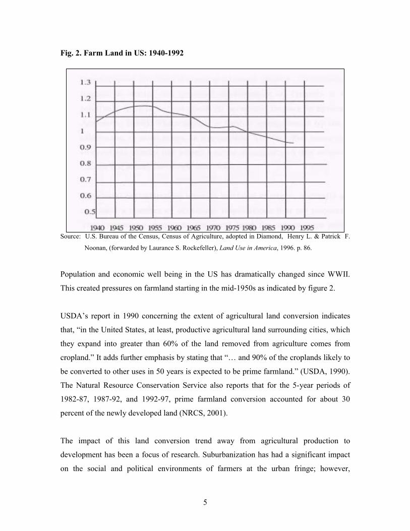
Fig. 2. Farm Land in US: 1940-1992
Source: U.S. Bureau of the Census, Census of Agriculture, adopted in Diamond, Henry L. & Patrick F.
Noonan, (forwarded by Laurance S. Rockefeller), Land Use in America, 1996. p. 86.
Population and economic well being in the US has dramatically changed since WWII.
This created pressures on farmland starting in the mid-1950s as indicated by figure 2.
USDAs report in 1990 concerning the extent of agricultural land conversion indicates
that, in the United States, at least, productive agricultural land surrounding cities, which
they expand into greater than 60% of the land removed from agriculture comes from
cropland. It adds further emphasis by stating that and 90% of the croplands likely to
be converted to other uses in 50 years is expected to be prime farmland. (USDA, 1990).
The Natural Resource Conservation Service also reports that for the 5-year periods of
1982-87, 1987-92, and 1992-97, prime farmland conversion accounted for about 30
percent of the newly developed land (NRCS, 2001).
The impact of this land conversion trend away from agricultural production to
development has been a focus of research. Suburbanization has had a significant impact
on the social and political environments of farmers at the urban fringe; however,
5

6
relatively little is known about its economic impact on agriculture (Lopez, Adelaja, and
Andrews, 1988). The concern is further strengthened by the fact that land converted to
other uses, in most cases, is irreversible. The fact that many current land use choices have
irreversible effects has added a sense of urgency to this subject (The North East Regional
Center for Rural Development, 2002).
Continual and alarming rates of land use changes, especially away from agricultural uses
can have a number of economic implications that are important for policy consideration.
The competing demands for rural land for urban uses lead to a gradual diminishing
supply of prime agricultural land. As a result, land brought into production to compensate
for farmland losses is often of lower quality, and is marginal in agricultural productivity
(Ramsey and Corty, 1982).
Fig. 3. Land Use Changes in United States: 1982 - 1992
Source: U.S. Soil Conservation Service, National Resource Inventory, 1992., adopted in Diamond, Henry L. & Patrick F. Noonan,
(forwarded by Laurance S. Rockefeller), Land Use in America, 1996. p. 86.
The National Resource Inventory similarly reports particular concern on the effect of
agricultural land conversion on croplands. Figure 3 shows the change in land use in one
decade (1980-1990) in the United States and shows the relative change in agricultural
land use in the stated period.

Although agricultural land preservation policies increased the total quantity of
agricultural land in the period, development pressures impacted the state of agricultural
land, particularly cropland, which by their very nature are typically prime farm lands.
Development of adjacent agricultural lands can also interfere with the efficiency of
farming practices. With increasing rural land development, consequent demand for public
facilities arises and claims even more land. Regulation of farming practices and increased
property taxes as well as speculation on land can reduce farming practices and their
efficiency. As prime farm land shrinks and the need of land for non-agricultural uses
accelerates over time, the quality of farm family life disappears and the values that spring
from living close to that land is diminished. The quality and rate of conversion of rural
land affects not only the productive capacity of food and fiber, but it also affects the rural
economies, environmental quality, and other socio-economic activities.
The trend of agricultural land development has triggered public policy debate on land use
management. However, the agricultural land policy debate has centered on the adequacy
of the land base to provide food and fiber at some "reasonable price" in the future
(Brewer and Boxley, 1981). This is a valid national concern, but exclusive attention to
this issue has obscured the more widespread and immediate national concern over land
use change and agriculture in urbanizing areas (Platt, 1985; Anderson, et al, 1975). In
view of the urgency of the matter and public concern, it is important to study the problem
more closely and understand the complex interaction and effect of the existing conversion
challenges to economic systems and social welfare in the coming generations. Closer
investigation of the issue can provide more information to policy makers and decision
makers in land use planning decisions.
This study focuses on the nature and implications of the land conversion situation in West
Virginia. Development of rural lands to other uses indicates a permanent loss of scenic
views, open space, wildlife habitat and rural life style. Some studies indicated increased
use of land for residential, commercial, industrial, extractive, and recreational uses and
for transportation, public utilities, community facilities, and government installations
7

(State MRP Land Use Committee, 1976; Tall and Colyer, 1989). The Census of
Agriculture 1992 also reported that the total number of farm acres in West Virginia
declined by over three percent from 3.37 million acres in 1987 to 3.27 million acres in
1992.
A substantial amount of land in and around the small towns and their constituting
counties located near large centers, particularly in the eastern Panhandle, is being used
for second or retirement homes, campground and weekend recreational use, or has been
purchased for profitable investments. Most of these developments seek flat, well-drained
land. However, the quantities of such land, which are usually used for farming, are
severely limited in most West Virginia communities. As a result, such losses of land
make it difficult or impossible to maintain rural land for agricultural uses because returns
to land in agriculture are low relative to other uses in West Virginia (MRP, 1976).
Agricultural technologies compensated in many other states by increasing yields and
lessening the impact of conversion of land from being noticed. However, the revolution
in agricultural production techniques creates a disadvantage for areas such as West
Virginia. A large proportion of the land is steeply sloped, with the most productive land
being converted to housing, commercial, or industrial uses. Since returns on land in
agriculture are low relative to other land uses, specific policies are needed to protect the
remaining agricultural areas.
From the economic perspective, a major criticism of agricultural preservation measures is
that they are based on limited information about the impacts of sub-urbanization on
agricultural production and income (Gardner, 1977). Hence, a study of the conversion of
agricultural land in West Virginia is an important task and may shed light as to the extent
of the problem and alternative land management schemes in the state.
It is finally appropriate to comment that understanding the balance between humans and
nature with all the complex interactions is a timely and wise endeavor, as Donald Worster
(1993) beautifully suggests that: the way we use the land reflects our understanding of
8

nature and our perception of ourselves. If widespread degradation is an indication that our
understanding of nature is narrow, it also suggests that so too is our perception of our
own role in the functioning of natural system. (quoted in Diamond and Noonan, 1996).
1.2. GENERAL REVIEW OF PREVIOUS WORKS
Conversion of agricultural land to urban uses is a phenomenon currently affecting
countries as population growth, existing agricultural practices and shifts in economic
activity interact dynamically. Suburbanization, which is characteristic of many regions of
the US, has been accelerated in the post war period by federal tax policies that subsidized
single family housing and state and local highway construction. As a result, housing and
their infrastructural development have occurred in predominantly agricultural areas
(Lopez, et al, 1988).
More recently, urban land has increased by 2.4 million acres from 1970 to 1980. Defined
metropolitan land areas increased by 60 percent between 1970 and 1985 and recently
encompassed 16 percent of U.S. land (Heimlich and Reining, 1989). Barkley and
Wunderlich (1989) added that a 1988 survey showed that 3.5 percent of rural land
transferred each year, of which 88.4 percent is agricultural land. Likewise, the Census of
Agriculture (1992) reported that areas in the United States increased by 30 million acres
from 25.5 million acres in 1960 to 55.9 million acres in 1990. According to Pimentel and
Giampietro (1994), over the next 60 years urbanization will diminish the U.S. arable land
base of 470 million acres.
Public facilities encouraged by a growing population also claim a significant proportion
of agricultural land. Over the past 200 years, for instance, the expansion of these systems
has covered 260 million acres, approximately half of which was arable land (Berry,
1978).
There are different theories explaining what forces drive land conversion. One factor
focuses on the difference in rates of return from land due to its use and its relative
location as explained by Von Thuenen location theory. The conversion process presented
9

by R.F. Muth based on this theory suggests that land use patterns and the market price of
land are established by relative rental gradients for urban and agricultural uses.
Conversion of land to urban uses proceeds in concentric circles around a central city;
then, at the equilibrium boundary between urban and agricultural uses, relative rents of
competing uses are equal. Policy changes that favor suburbanization and growing
housing demand associated with population growth shift the urban and rural rent gradient
so that the equilibrium boundary moves away from the city center. Land speculation can
cause the market value of agricultural land to rise above the agricultural use value before
conversion if the expected urban rent at the conversion date over the planning horizon
exceeds the current agricultural rent (Lopez, et al, 1988).
The implications of this theory of land conversion have resulted in diverse analyses and
understanding among different concerned scholars and policy analysts. For instance,
Krupa and Vesterby (ERS) concluded that contrary to popular opinion, urbanization
does not necessarily mark the end of agriculture in rapidly growing counties. Farmland
does tend to decrease in counties where rapid population growth is sustained over several
decades. But changes in crops to high value fruit and nut; vegetables; and nursery and
green house products more than compensate for losses of other crops in real market
value. These changes can be attributed in part to the adaptive nature of agriculture...
(Krupa & Vesterby, 2001, p.11).
However, many still insist that there are a number of direct and indirect implications that
are not fully compensated during the conversion process. Vesterby, et al. (1994) raise
issues revolving around the value of land that may fail to be accounted for in the
valuation process. Aside from issues of productivity of the agricultural sector impacted
by conversion processes, urbanization of rural land does raise issues at the State and local
levels with regard to protecting watersheds, maintaining air quality, providing open
space, preserving rural life styles, preventing urban sprawl, and preserving local
economies. These values are usually not internalized in the market price of farmland.
10
Many studies also measure the direct effects of the loss of farmland to urban uses in
terms of output reduction and income losses. Indirect impacts on the farming community
could also include regulatory restrictions on farming practices with sub urbanization,
technical impacts, and speculative influences. When farmers become uncertain about the
future viability of agriculture in their area, farmland production falls, as does farming
income. Ultimately, the critical mass of farming production needed to sustain the local
farming economy collapses (Berry 1976; Daniels and Nelson 1986; Daniels 1986;
Lapping and Fitzsimmon 1982).
Farmers can also face insecurity in their future operation that may lead them to reduce
investments in farming. They may also await conversion of their land to other non-
agricultural uses - an effect called the impermanence syndrome. Land use policies,
therefore, should address the impermanence impact on the agricultural sector vis-à-vis
land management schemes.
Hence, understanding the full impacts of alternative land management policies and the
existing relationships between urban and rural agricultural land allocations is key to
addressing the land use challenge.
1.3. OBJECTIVES OF THE STUDY
The general objective of this study is to measure the direct and indirect effects of
migration on farmland conversion in West Virginia. Specifically, the objectives are to:
1. Model the effect of population changes on agricultural land conversion.
2. Model the effect of employment changes on agricultural land conversion.
3. Model other factors associated with population and employment changes and
agricultural land conversion.
1.4. METHODS OF ANALYSIS
This study will use extensive descriptive and qualitative analysis. To facilitate the
understanding of descriptive relationships in land use processes, extensive secondary data
11
is collected. This will provide an initial understanding of the extent of the problem in
West Virginia and possible trends.
Secondary data is collected from different sources including the US Census of
Agriculture, County and City Data Books, REIS, and on-line sources.
The database will also provide a base to undertake econometric analysis to understand the
effects of suburbanization on agricultural lands. Particularly changes in population,
income, employment, land in farming and other competing uses, and geographical
location aspects and accessibility information will be relied upon for econometric
evaluation of the problem.
This study will typically employ an econometric model following the Carlino-Mills
Growth Model with relevant adjustments to address the objective of this study. This
model was initially used to explore the determinants of population and employment
densities inter-regionally. The model uses changes in employment and population with
other relevant exogenous variables to explain county growth by estimating a system of
equations model using two-stage least-squares method (TSLS) (Carlino & Mills, 1987).
This general growth model has been applied in different studies for different purposes by
making adjustments to the original model. For instance, Deller et al. (2001) employed the
Carlino-Mills model to study the role of amenities and quality of life in rural economic
growth, and in Duffy-Deno (1997) to study the economic effect of endangered species
preservation in the non-metropolitan west.
1.5. ORGANIZATION OF THE STUDY
This thesis consists of five distinct chapters. Chapter One provides a general introduction
to the statement of the research problem, the objectives, methods of analysis and a
general review of the land use literature. It also introduces the research ideas and
direction. Chapter Two provides an overview of the land use theories development and a
microeconomic theoretical framework for land use decision processes and optimal
location and land size considerations by economic agents. It provides the necessary
12

theoretical intuition for the specified model. Chapter Three builds the empirical model
with detailed specification of the variables of the model. It specifies a system of
equations growth model to estimate the change in economic and demographic factors on
agricultural lands. Chapter Four focuses on the presentation and analysis of the empirical
results generated from the specified model. Finally, Chapter Five will provide a summary
of the research.
13

CHAPTER II
ECONOMIC THEORY OF LAND RESOURCE
ALLOCATION, USE, AND CONVERSION
2.1. BACKGROUND
Economics, as a formally organized and scientific field, has been expanding and
encompassing numerous areas of interest since the time of Adam Smith. Though basic
questions of what to produce, how to produce and for whom to produce are general
concerns of every society from the earliest times history can record, a concise and more
scientific approach to address such general and numerous specific societal questions has
grown in the past few centuries.
As a particular field, economics has been dealing with resource use and allocation
problems. Economic resources bounded by the natural, physical, and technical growth
constraints on the one hand, and growing human insatiable needs on the other has created
pressure on the use and allocation of scarce resources.
Knowledge in the understanding and management of natural environments and all
endowed resources has increased throughout human history. However, global population
increases, unwise and unsustainable resource utilization practices, distorted allocation
policies, and alarmingly growing new human needs and the justifiable desire to maintain
an already achieved economic status have all engendered further pressure on the use of
scarce economic resources.
Economic resources have different characteristics requiring different methods of
management and distribution. It is generally true that resources are bound to economic
forces of demand and supply in determining their value and distribution once they are
made accessible to the market. However, specific behavior of resources and their relative
14

abundance will also play a significant role in determining the value and distribution of
those resources.
Of the four factors of production, the land resource has a peculiar characteristic of zero
price elasticity in physical supply and a high opportunity cost in economic supply.
Among other reasons, this coupled with physical immobility make the determination of
its value and distribution different from other factors.
Labor mobility within and across nations, some degree of capital mobility, and the
freedom of entrepreneurs to locate in areas of high incentive and productivity have all
played roles in price adjustments and value convergence among economic resources
across space. Land, however, is constrained by its physical immobility or spatial fixity in
alternative economic use which consequently limits value adjustments across space in its
wider dimension. Hence, it is no wonder that land resources have captured the interest of
many economists since the pre-Classical economics period.
In Neo-classical microeconomics, though it is possible to subject land to a general frame
of marginalist analysis, its specific physical behavior and high opportunity costs of
conversion to alternative uses by themselves deserved a cautious approach. This is one
fundamental reason why policies related with land reform, reallocations as well as free
market distribution, permit the coordination and redirection of trends in land use practices
through regulations and/or different incentive schemes.
More recently, the sustainable use of land between different competing economic
activities along with an understanding of implications for coming generations is receiving
growing attention. As land use changes affect not only land, per se, but also on the
environment and other natural amenities, its analysis within a comprehensive sustainable
economic framework is a definite requirement.
Though markets are an ambiguously efficient means of resource distribution under
certain assumptions, failure of markets to address the crucial issues of externalities and
15

16
sustainability in natural resource allocation can result in adverse long-term consequences;
as Theodore Roosevelt, 26th President of the United States, beautifully puts it:
To waste, to destroy our natural resources, to skin and exhaust the land instead of using
it so as to increase its usefulness, will result in undermining in the days of our children
the very prosperity which we ought by right to hand down to them amplified and
developed5.
This chapter generally deals with the genesis of economic theory of land value and
allocation from the pre-Classical period to the Neo-Classical marginalist approach to
understand the root and further developments in land use and allocation economics. It
also includes an application of a neo-classical framework for the determination of goal
maximizing location preferences. This will provide a sound theoretical foundation for the
econometric analysis in this thesis.
Through time, land has been converted to different uses for different economic,
technological, institutional, legal, and policy reasons. The conversion of land across
sectors, however, is not without implications to environmental quality, income growth,
and welfare changes across sectors. Of particular interest for this study is the conversion
of agricultural lands to nonagricultural uses. This conversion process through time could
have implications on quality of life, preservation of environmental and other natural
amenities, farm income, sustainable agricultural production, as well as on public interests
of open space, farming tradition, and landscape preservation standards.
5 Quotation adopted from http://www.stthomas.edu/recycle/land.htm

2.2 GENERAL REVIEW OF EARLY LAND RENT, USE, AND ALLOCATION
THEORIES
Land rent and use issues have been focal points for theoretical development in the early
pre-classical, classical, and neoclassical periods of economics. Although the nature of
land issues change from period to period and from generation to generation, some
fundamental attributes of land value and use were investigated at some depth. Most
earlier studies in the area starting in the 17th century focused on agrarian land uses.
Recently, with societal transformation to more industrial and service economies,
differential land rents and competing uses has gained more attention.
Though limited in depth and focus of analysis, pre-classical analysts had devoted time to
investigating the value and use of land. Some even consider that land-rent first became
area of vigorous theoretical interest for the works of the seventeenth-century mercantilists
(Keiper, et al., 1961).
This period revealed early theoretical interest in the theory of value, particularly in the
development of an early rent concept in land and labor. Generally, land use theories in
this period can be inferred from the works of prominent contributors of the period.
William Petty, one such contributor, states that the extrinsic value of land may be derived
by taking the average of all bargains undertaken at a definite given time period (Wilson,
1894). He summarizes value as one that is generated from a net return on the use value of
land and the other aspect depending on average bargaining value which could be
influenced by the market condition. On the relationship between land value and
population, Petty argues that rent of land near places of high population increases due to
the honor and satisfaction of having land there (Keiper, et al., 1961).
Cantilon demonstrates that the allocation and use of land depends on the return different
activities promise to bring to that land (Cantilon, 1755). Similarly, Turgot addresses the
same question in his argument that competition sets the price of leases of land (Turgot,
1770).
17
Classical Period economists generally measured value in terms of labor cost which
entered extensively in international trade analysis based on comparative labor cost
advantages and production and distribution issues. Extensive writings have also been
made in land rent theories and allocations.
One of the contributors to classical land rent theory is Adam Smith, whose work greatly
shaped economic thinking of his period and laid a foundation for the later development of
economics. Smith treats the rent of land as a monopoly price, it is not at all proportioned
to what the landlord may have laid out upon the improvement of the land, or to what he
can afford to take; but to what the farmer can afford to give. (Smith, 1776). His classical
land use theory takes into account the influence of competition between different
economic activities on land use and allocation as well as the role of distance and
transportation cost in land rent and use. The influence of distance from a particular city or
populous area on land rent is that rent not only varies with fertility of land but it also
varies with location. Land near a town gives a greater rent than land equally fertile in a
distant location. Though the production cost may not be different, the produce costs more
to bring it to the to the distant market (Ibid, 1776).
Smith argues that good transportation facilities like roads, canals, and navigable rivers
will diminish transportation costs and makes distant places more accessible. This
encourages the cultivation of the remote, which is the most expensive location of the
country (Ibid, 1776). With regard to land conversion between different uses, Smith states
that an acre of land will produce a much smaller quantity of the one species of food than
of the other, the inferiority of the quantity must be compensated by the superiority of the
price. If it was more than compensated, more corn land would be turned into pasture; and
if it was not compensated, part of what was in pasture would be brought back into
corn.(Ibid, 1776).
Another significant contributor to the theory of land rent in the classical period is David
Ricardo. His rent theory recognizes that there is an upward trend in human demography
and location friction, and competition for resources will create rent. In describing the
18

behavior of rents for fertile and surrounding marginal lands, Ricardian theory develops a
concentric circle type of analysis. With three types of land arranged according to their
fertility with 1 being the most fertile, the theory states that as the competition for
marginal lands increases, the rent for the more fertile ones will increase. As land of lesser
quality, say third quality, is put into use rent rises on the second by the difference of their
productivity. Similarly, the rent for first quality land will also increase since its rent is
greater than that of the second quality. As population grows, which shall force a country
to depend on worse quality land, rent on all fertile land rises (Ricardo, 1817).
An extension in Classical land theory is introduced by John Stuart Mill who brought the
concept of opportunity costs into the theory. Mill views land rent as the rent which any
land yields in excess of its produce beyond what would be returned to the same capital if
employed on the worst land in cultivation(Mill, 1848). This addition to rent theory
involves an element of opportunity cost as the rent of a given land is compared to
whatever is in excess if that capital is invested in poor land. Mill argues that the value
of goods that are scarce is entirely determined by demand and supply (Ibid, 1848).
Therefore, it can generally be concluded about the rent theories of classical economists
that the period reflected a tendency of rent theory genesis from Smiths and Ricardian
labour value based interpretations to a more complex and extended concept of Mill with
the introduction of opportunity cost.
As a break away from pure classical thinking of economic value and exchange, the neo-
classical period evidences a new paradigm of economic thinking. Bringing into the core
of economics the philosophical ideas of utilitarianism, it approaches consumer behavior
from a utility point of view and profit maximization motives from a business point of
view and generates a whole set of microeconomic behavioral analysis from that angle.
By 1866, one of the founders of the neo-classical thinking, William Javons, stated his
view of utilitarian economics that a true theory of economy can only be attained by
going back to the great springs of human action - the feelings of pleasure and pain.
19
(Javons, 1866). Under this micro-economic framework, exchange of goods and services
can occur to the extent where utility is successively created until a point where the
diminishing marginal utility will remove all utility incentives for a given price.
In contrast to classical theory of labor value, another founder of neo-classical economics,
Carl Menger, argues that value is not embodied in goods but rather on the satisfaction of
human needs (Menger, 1871). Neo-classical economics treats land as a commodity
subject to the forces of demand and supply. For instance, Menger argues that the
treatment of the value of land is not exceptional among goods. Menger argues that
whenever a question arises as to the determination of the value of land, it is subject to the
general laws of value determination (Ibid, 1871).
Similarly, Alfred Marshal argues the rent of land is no unique fact, but simply the chief
species of a larger genus of economic phenomena; and that the theory of the rent of land
is no isolated economic doctrine but merely one of the chief applications of a particular
corollary from the general theory of demand and supply (Marshall, 1890).
On the study of land conversion to different uses, Henderson developed the concept of
margin of transference. This concept states that land is at the margin of transference if
its rent is just sufficient to protect its being converted to other alternative uses (Keiper, et
al., 1961).
Today, with the transformation of the American economy from agrarian to industrial and
now services, as well as the improvement of communication technology and resulting
lower accessibility costs, the competition over a given convenient space is intense.
Business and residential location decisions expand to greater distances from the center of
the city or administrative centers. Though the allocation of land at a particular space and
with given natural features among different economic activities will follow the same
basic economic principles, the process, however, is by no means trivial.
20

The consideration of buying a piece of land for residence for instance can be treated the
same way as a consideration for the purchase decision of a common commodity in terms
of economic behavior. As Robert M. Haig argues in selecting a residence, one can be
thought as buying accessibility precisely as one buys consumer goods. One hence
compares location and resulting costs of friction, rent, time and commuting costs which
are matched with derived satisfaction and resources to place the consumption decision
(Haig, 1926).
Finally, households decide their location based on their utility maximization derive and
resources; producers make similar decisions of location based on their maximization
tendency. The point where these two forces balance determines location (Losch, 1954).
The trend in value and allocation theories indicate the transformation of economic
thinking from Classical labor value based approach to the marginal value based approach
of Neo-Classical Economics.
2.3. DEVELOPMENT OF EARLY BID-RENT FUNCTIONS AND LAND
ALLOCATION
Development of early bid rent functions and its early mathematical treatment is
associated with the work of von Thunen. Different economic historians and writers
attribute his work as an early sign of departure from classical thinking to neo-classical
thought, especially in the theory of distribution and application of marginalist analysis.
Von Thunens land allocation theory gives a more complete picture of the allocation
process by bringing competition and transportation savings in a mathematical bid-rent
function. Von Thunen starts with certain assumptions that could be relaxed to meet
reality. The assumptions ask to:
Consider a very large town in the center of a fertile plain which does not contain any
navigable rivers or canals. The soil of the plain is assumed to be of uniform fertility
which allows cultivation everywhere. At a great distance the plain ends in an uncultivated
wilderness, by which this state is absolutely cut off from the rest of the world. This plane
21

is assumed to contain no other cities but the central town and in this all manufacturing
products must be produced; the city depends entirely on the surrounding country for its
supply of agricultural products. All mines and mineral deposits are assumed to be located
right next to the central town. (Brooks, 1987).
The main concern under such a case is to determine how distance from the city affects the
efficient allocation of land for different economic activities. The model specifies that
each economic activity (in agriculture) can bid a rent at a particular location per unit of
land offering a bid the maximum of which is equal to the value of the product minus all
the costs of production, including transportation cost. Competition among producers
ensures that the actual rent bid will be the largest. Potential profit for any product
diminishes with distance at a rate equal to the transportation cost (Ibid, 1987).
Following Von Thunens argument, we can write the bid rent function in a simple
mathematical form as: Rn = pQ - wiXi - Dt where Rn is the net revenue per unit of land
from the products of that land situated at distance t from the central market, Q is output
and Xi is the set of all inputs needed to produce Q per unit of land, p and w representing
input and output prices per unit respectively and Dt denotes the cost of transporting Q to a
unit of distance. Rn can be viewed as the maximum any bidder can offer since it does not
make any economic sense to offer for a specific parcel of land at a specific location a bid
that is more than what that land is economically worth. Hence, it follows that any change
in input and output prices as well as any improvement in transportation technology is
going to affect the optimal allocation of land and effect the spatial feature of land uses.
(see Brooks, 1987).
To graphically generate a bid-rent function from Rn = pQ wiXi Dt, we may identify net
revenue (maximum bid) on the vertical axis and distance on the horizontal axis. Thus, by
taking the intercepts we can draw the bid rent function (figure 4).
22

Fig. 4. Bid Rent Function for Land situated at a certain distance.
Rn
pQ-wX
0 (pQ-wXi) / t t It can be noted from the bid rent function that changes in input and output prices as well
as improvement in transportation technology can affect net revenue. This results in
different bid rent functions for different economic activities and will result in different
spatial land use distributions.
Following Von Thunens concept of concentric circle analysis, it is possible now to see
what happens if more than one activity on a parcel of land occurs under conditions of full
competition. For a three-crop example in agriculture, Fig. 5 indicates the allocation
pattern that can result. Assume three crops A, B , and C compete over a favorable
location. Lets assume now that Rn A > Rn B > Rn C Qi > 0; where Rn is net revenue
(maximum bid). It is evident that with distance and constant transport technology and
input and output prices, the net revenue of A, B, and C diminishes as distance from a
market increases as transportation cost saving declines. Hence, the land will be allocated
in such a way that A bids out locations near the center followed by B and C as shown in
figure 5. The crop offering the highest net revenue at a given location will outbid other
activities and the land will be put to that use. However, it is clear that relaxing the
assumptions of a constant technology coefficient and constant input and output prices, the
land use pattern will be varying and dynamic over space, although the same behavioral
pattern can generally be captured.
23

Fig 5. Bid Rent functions of Three Agricultural Activities and Land Distributional Pattern
Source: Adopted from http://faculty.washington.edu/~krumme/450/exercises/landuse.gif
An interesting issue will arise when consideration is given to differential rents arising
from spatial competition involving different sectors. Though the same principle applies, a
general concentration of sectors across space may be observed for reasons of higher
returns in certain sectors per given distance and agglomeration economies. Fig 6
demonstrates a hypothetical land use distribution across three sectors. It shows that retail
activity will prevail over space up to a concentric circle with radius of d1 and
manufacturing within a distance of d2-d1 from the central market and residential
concentrations in the area d3-d2. For the whole distance 0d3 the upper margins of the
bid rent functions forms the rent gradient.
Viewing the allocation process dynamically, the market price for each product is
simultaneously determined and depends not only on its supply and demand condition, but
also on the prices of other goods and services associated with it. Thus, the supply and
spatial location of agricultural industry depends on its price and prices of other goods
(Ibid, 1987).
24

Fig 6 Bid tion
. Rent Functions of Three Sectors and Resulting Land Distribu Pattern
ource: http://www.uncc.edu/~hscampbe/landuse/b-models/C-bidrent.html
2.4. ECONOMICS OF LAND USE, ALLOCATION, AND CONVERSION
As discussed in section 2.2, the study and understanding of land rent, use, and allocation
has been the concern of theoretical study for a long time. However, a deeper
nderstanding of the land use process with changing individual and societal economic
eeds across space is still creating economics modeling and policy challenges.
ial
growth. It is a zone of mixed land-use elements and characteristics in which rural
also commercial, educational, recreational, public service and other largely extensive
inistrative, sense too, the
area is only partially assimilated into the growing urban complex. (Thomas, in Johnson,
S
u
n
This study deals with the conversion of agricultural lands to non-agricultural uses,
especially at the urban fringe. Urban fringe is meant as the:
underdeveloped space into which a town or city expand by circumferential or rad
activities and modes of life are in rapid retreat, and into which not only residential, but
uses of land are intruding. In a land-use, and often in an adm
ed., 1974).
25

Throug ention
because partly
because new construction activities in the city pose architectural preservation questions.
n the other hand, changes on the edge of the city are related with the conversion of land
ities due to scattered and
nplanned rural development, frictions in land use, deterioration of environmental
rueckner and Fansler, 1983,
. 479). In many cases, the positive externalities of the rural sector are not accounted for
l benefits from agricultural lands such as open space,
nvironmental quality, and impediments to urban sprawl. Many of these benefits have
h time, the change in spatial features in the cities has received greater att
the redevelopment of inner cities addresses difficult social problems and
O
to urban uses. This could involve basically a greater alteration than other forms of land
use changes taking place in urban areas. (Johnson, ed., 1974).
This new spatial feature definitely creates friction among economic sectors in their
competition for land as well as on social and environmental interactions. This, however,
increases societal costs in terms of increasing costs of amen
u
quality, disruption of local production methods and farming practices, and transformation
of rural landscapes into urban type developments. Suburban developments also affect the
value of agricultural land and different use competitions can reduce the effectiveness of
the agricultural sector. In many cases, conversion processes do not account for
externalities associated with land conversion and as such their long-term implications to
societal welfare should be properly gauged and understood.
Consequently, through the transformation of pastoral farmland into often-unattractive
suburbs, sprawl is thought to disrupt a natural balance between urban and non-urban land
uses, leading to a deplorable degradation of the landscape (B
p
in the value of the converted land to other uses. Irwin and Bockstael suggest in their
estimation of open space spillovers using a hedonic pricing model of residential property
sales that the positive amenity value associated with open space may not be identified.
(Irwin and Bockstael, 2001).
From a policy perspective, the conversion of agricultural lands to non-agricultural
(development) uses has been a critical public issue. In recent years, attention has
focused on preserving loca
e
26

public characteristics and, as a consequence, will tend to be undersupplied by private
producers (Plantinga and Miller, 2001, p. 56).
Understanding the forces behind land conversion to non-agricultural uses is particularly
relevant in modeling and predicting land use changes. Pressure on agricultural land can
generally be seen from the rural agricultural sector point of view as well as from city
ressure points of view to explain the origin and effect of factors of conversion.
time and
ace, however, are a number of theories trying to identify the possible sources of factors
or
burbanization. In the 1960s, the interstate highway system and racial tensions were
ay be demanded for direct consumption needs as in housing or for manufacturing and
p
With increases in urban population and residential and employment preference towards
the edge of cities, the conversion process becomes eminent unless interrupted by policy
measures. Behind the forces of population and employment changes across
sp
affecting the suburbanization process. One class of theoretical explanation for
suburbanization stresses fiscal and social problems of central cities: high taxes, low
quality public schools and other government services, , crime, congestion and low
environmental quality. These problems lead affluent central city residents to migrate to
suburbs, which induces further out-migration (Mieszkowski and Mills, 1993, p. 137).
In the context of the United States, different reasons are generally attributed as causing
suburbanization pressures during different decades. During the 1950s, it was claimed that
home mortgage insurance by the federal government was responsible f
su
popular explanations of decentralization. More recently, crime and schooling
considerations have been prominent explanations of urban decentralization. (Ibid, 1993).
Although land development pressures can be seen from a different perspective,
theoretically they can be generalized in a microeconomic framework of utility and profit
maximization motives with location and land size being relevant decision factors. Land
m
other commercial purposes.
27

In the case of private housing demand for land, open space is often cited as a primary
attractor of urban and suburban residents to exurban areas located just beyond the
metropolitan fringe. Included in the rural amenities afforded by open space are scenic
iews, recreational opportunities, and an absence of the disamenities associated with
havior may be summarized by households compensated demand functions
efined by the level of utility achieved under prices P(t)). Land not being used in the
roblem. In a two industry analogy, arranging zones and industries can be
rranged in an increasing distance from centers such that the ith industry occupies zone i
d uniform
cross the region. The equilibrium condition requires that for the ith industry to occupy
one i, its bid rent mu rent is required at least to be
introduced into the system. Among other factors, population growth and employment
v
development, such as traffic congestion and air pollution. (Irwin and Bockstael, 2001, p.
668).
Mills argues that that households endowed with perfect knowledge of P(t), the vector of
residential service prices at time t, select the residential service that maximizes their
utility. This be
(d
provision of residential services is taken up by some unspecified alternative use. (Mills,
1978, p. 228).
In the case of industrial and other commercial demand for land, generally locations that
minimize costs and help maximize profits are desired. Miyao provides a general approach
of the location p
a
(i = 1, , m). In the long-run competitive equilibrium, satisfying the long-run zero profit
condition, the ith industry bid rent at distance x can be expressed as ri(x),
Ci[ri(x),w] = pi qi(x) (i= 1, , m)
where Ci, pi, qi, and w are the ith industrys per unit production cost, output price and per
unit transport cost, and the wage rate respectively. The wage rate is assume
a
z st be one of the highest, i.e., the bid
equal to other industries everywhere in the zone; i: ri(x) ≥ rj(x) for all j = 1, , m.
(Miyao, 1977).
Within these general frameworks, a number of relevant factors of influence can be
28
expansion are relevant factors in influencing the land conversion process. They
simultaneously interact to influence one another and the demand for land across different
nd uses.
density at the edge of the CBD, and is the gradient or the constant
ercentage change in the population density per unit change in distance from the CBD.
nd conversion from rural to urban uses have intensified concern among
any persons. (Muth, 1961).
s. (Fisher, 1956).
rbs indicates that the decentralization of
sidential places from the central city is followed by the decentralization of employment.
la
Brueckner shows that under certain simplifying assumptions about preferences and
technology, population density is shown to have an exponential form (Brueckner, 1982),
D(θ) = D0e-θ, where θ is the distance from the CBD (Central Business District), D0 is the
population
p
(Brueckner, in Mieszkowski and Mills, 1993, p. 138). However, with expanding
population, greater distances from the city edge are brought under settlement
consideration.
Barlowe argues that irrespective of the opinion one holds on the ambigeous question of
population control, it need to be understood that the population growth pressure has a
significant impact on the demand for land and its products (Barlowe, 1958). Consequent
problems of la
m
With increasing suburbanization, need arises in the suburban areas to develop socio-
political and economic institutions, transport and public utility infrastructure, health and
education services and other attendant social needs facilitating the conversion of land to
more intensified suburban use
Simultaneously interacting, employment also plays a major role in affecting land use
patterns over space and in affecting the conversion of land away from agriculture.
Though direction of causation between employment or population is a debatable issue,
the Natural Evolution Theory of cities and subu
re
Hence, firms moved to the suburbs following the change in population location
preferences, to provide services and to benefit from lower suburban land and labor costs.
29
However, the movement of employers to suburban areas further stimulates a change in
population across regions as employees followed them. (Mieszkowski and Mills, 1993).
Generally, in a competitive land market the price for land equals the present discounted
value of the stream of future rents. Thus, if rents from development exceed agricultural
rents in the future, the higher rents from future development will be capitalized into the
current price of agricultural land. (Plantinga and Miller, 2001). Hence, as the
evelopment pressure intensifies following the out-migration of population and
d use issue.
other variables of interest
presented as:
rent, y is income and t is per round-trip mile commuting cost. The result
stablishes that with the increase in the urban population, the edge of the city must
expand as the need ar ase in agricultural land
nt raises the opportunity cost of urban land relative to agricultural land and results in a
more compact city. An increase in income increases the demand for housing and results
d
businesses to suburban areas, more land will be put into use for housing and development
purposes as these economic activities might provide a better bid than competing
agricultural and other rural economic activities.
From a theoretical perspective, establishing a sound relationship among factors that
interact in the land conversion process is crucial. Understanding such interplay of
locational (spatial) objective maximization decisions of households and businesses
provides a microeconomics perspective of the lan
Some studies provide a microeconomic approach to land use issues and establish relevant
relationships between economic behaviors and location in a comparative static analysis.
For example, Brueckner and Fansler provide comparative static emphasis of Wheaton
(1974) indicating specific relationships between distance and
re
x/L > 0, x/ra< 0, x/y > 0, x/t < 0,
where x is the distance to the urban-rural boundary, L is the urban population size, ra is
agricultural land
e
ises for more people to be housed. An incre
re
30

31
in an expanding city margin. Finally, a rise in per mile commuting cost lowers disposable
income at any given location, and hence reduces housing demand which results in less
pressure towards city edges. (Brueckner and Fansler, 1983).
Similarly, Plantinga and Miller provide a discussion of the competitive land market study
of Capozza and Helsey (1989). The model provides equilibrium rents from developed
land as: - - R(t,z) = A + rC + (T/L)[z(t) z]
where A is a constant annual agricultural rent, T is commuting cost, L is a fixed land
requirement, z is distance to the city center, and z(t) is the distance from city boundary to
a city center. The comparative static results establish that development rents are rising
through time at a fixed location (R(t,z)/t > 0) resulting from population pressures.
Population growth expands the city boundary (z(t)/ t > 0) and confers location rents on
existing developed land. With an increase in distance away from the central city,
development rents decline (R(t,z)/ t < 0) due to the falling of rents to offset increasing
commuting costs. (Plantinga and Miller, 2001).
Therefore, though a microeconomic framework provides a general theoretical base to
analyze land use changes, the inclusion of employment, population, commuting costs,
distance from urban center, farm rents, developments prices, and many more variables of
interest within the general microeconomics and regional growth realm are all relevant and
can enrich the understanding of land use changes and allocation frictions.
2.5. MATHEMATICAL ANALYSIS OF LAND USE DECISIONS AND
ALLOCATION IN A MICROECONOMICS FRAMEWORK6
So far, the general theoretical reasoning behind the guiding economic principles of land
use and allocation has been discussed. Among other things, a decision to locate at a
specific place can be affected by prices, transport technology, location preference, degree
6 For detailed mathematical and graphical analysis refer to Alonso, (1964).

of competition, legal systems, population pressures, degree of reg
ment policies, and so forth.
ional growth,
govern
s exogenous. For the purpose of current analysis, we
an limit the demand for land to commercial, residential and agricultural purposes and
t through transportation costs. In the case of
gricultural businesses, to simplify the analysis, lets assume that fertility is constant over
ortation
from arket.
Where π = total profits
L = land cost
Land can be allocated to lots of purposes starting from government institutional
requirements to purely commercial ends. The decision to place government institutions
and public facilities at a particular location rests on a lot of social and economic factors
and in most cases can be viewed a
c
see how pressures like population and business and employment expansion affect the
agricultural sector or land in agriculture.
2.5.1. Mathematical Consideration of Land-Use and Location Decisions by
Businesses
Lets assume that the objective of a given firm is to maximize profit by taking into
account the effect of location on profi
a
a given location so that the factor entering into the decision is the cost of transp
the nearest m
Then, following the theoretical microeconomic framework of Alonso, (1964), it is
possible to characterize the behavior of a profit maximizing firm mathematically as:
(1) Max π = R - C L
R = total revenue
C = total operating costs
32
A th t hand side variables are alsoll of e righ some function of distance and land size.
ubstit ing w e relationship as:
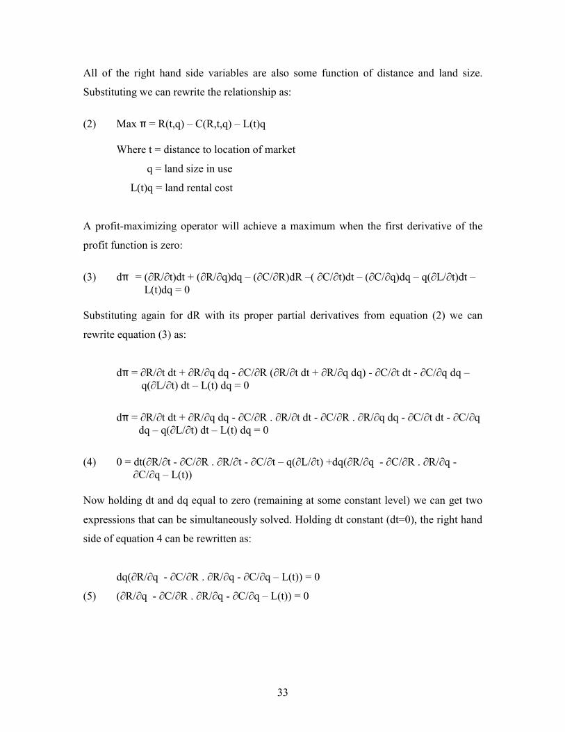
) Max π = R(t,q) C(R,t,q) L(t)q
Where t = distance to location of market
q = land size in use
profit-maximizing operator will achieve a maximum when the first derivative of the
(∂C/∂R)dR ( ∂C/∂t)dt (∂C/∂q)dq q(∂L/∂t)dt
ubstituting again for dR with its proper partial derivatives from equation (2) we can
dπ = ∂R/∂t dt + ∂R/∂q dq - ∂C/∂R (∂R/∂t dt + ∂R/∂q dq) - ∂C/∂t dt - ∂C/∂q dq
dπ = ∂R/∂t dt + ∂R/∂q dq - ∂C/∂R . ∂R/∂t dt - ∂C/∂R . ∂R/∂q dq - ∂C/∂t dt - ∂C/∂q
) 0 = dt(∂R/∂t - ∂C/∂R . ∂R/∂t - ∂C/∂t q(∂L/∂t) +dq(∂R/∂q - ∂C/∂R . ∂R/∂q - ∂C/∂q L(t))
remaining at some constant level) we can get two
xpressions that can be simultaneously solved. Holding dt constant (dt=0), the right hand
side of
(5) R/∂q - ∂C/∂q L(t)) = 0
S ut e can rewrite th
(2
L(t)q = land rental cost
A
profit function is zero:
(3) dπ = (∂R/∂t)dt + (∂R/∂q)dq L(t)dq = 0 S
rewrite equation (3) as:
q(∂L/∂t) dt L(t) dq = 0
dq q(∂L/∂t) dt L(t) dq = 0
(4
Now holding dt and dq equal to zero (
e
equation 4 can be rewritten as:
dq(∂R/∂q - ∂C/∂R . ∂R/∂q - ∂C/∂q L(t)) = 0
(∂R/∂q - ∂C/∂R . ∂
33
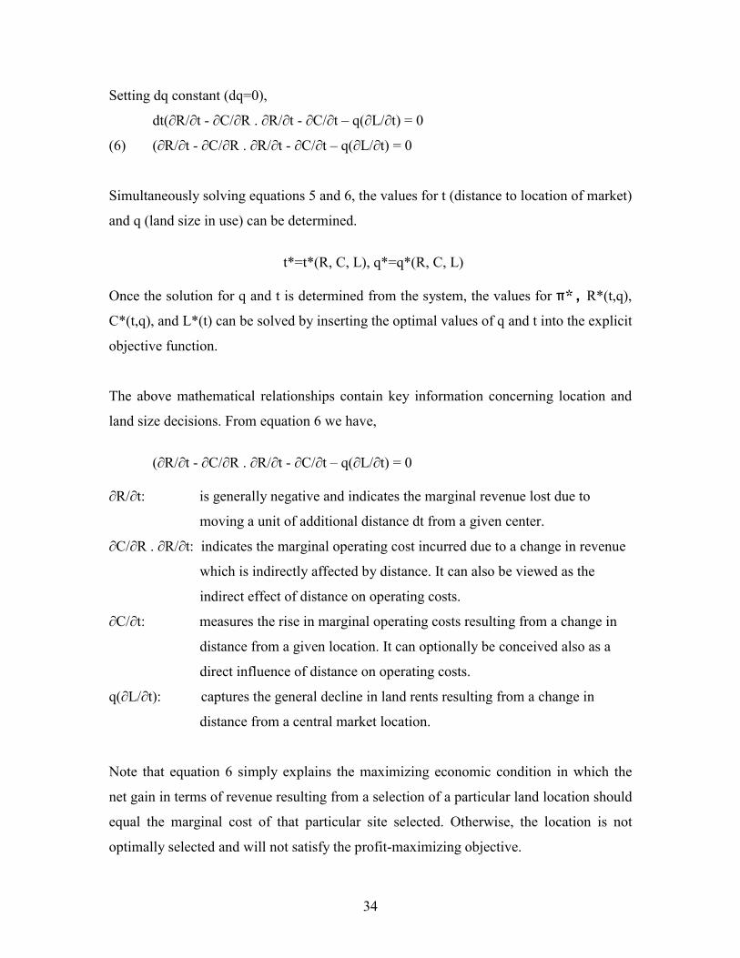
Setting dq constant (dq=0),
imultaneously solving equations 5 and 6, the values for t (distance to location of market)
nd q (land size in use) can be determined.
C, L)
t ystem, the values for π*, R*(t,q),
*(t,q), and L*(t) can be solved by inserting the optimal values of q and t into the explicit
he above mathematical rela on concerning location and
land size decisions. From equation 6 we have,
ly negative and indicates the marginal revenue lost due to
moving a unit of additional distance dt from a given center.
istance. It can also be viewed as the
s.
C/∂t: measures the rise in marginal operating costs resulting from a change in
d
rwise, the location is not
dt(∂R/∂t - ∂C/∂R . ∂R/∂t - ∂C/∂t q(∂L/∂t) = 0
(6) (∂R/∂t - ∂C/∂R . ∂R/∂t - ∂C/∂t q(∂L/∂t) = 0
S
a
t*=t*(R, C, L), q*=q*(R,
Once he solution for q and t is determined from the s
C
objective function.
T tionships contain key informati
(∂R/∂t - ∂C/∂R . ∂R/∂t - ∂C/∂t q(∂L/∂t) = 0 ∂R/∂t: is general
∂C/∂R . ∂R/∂t: indicates the marginal operating cost incurred due to a change in revenue
which is indirectly affected by d
indirect effect of distance on operating cost
∂
distance from a given location. It can optionally be conceived also as a
direct influence of distance on operating costs.
q(∂L/∂t): captures the general decline in land rents resulting from a change in
distance from a central market location.
Note that equation 6 simply explains the maximizing economic condition in which the
net gain in terms of revenue resulting from a selection of a particular land location shoul
equal the marginal cost of that particular site selected. Othe
optimally selected and will not satisfy the profit-maximizing objective.
34

Information concerning the plot size decision can similarly be generated from equation 5.
holds general information about the influence of land size on revenue and cost both
ffect of land size on the cost of production.
C/∂q Captures the change in cost caused by a unit change in the size of land
s generally positive. It is the direct effect of
from
omparative Statics Considerations
,
s well as a number of regulatory and institutional factors can
ffect the cost and revenue structures as well as the value of land. This will dynamically
activities. Though dynamics is beyond the intent of
It
directly and indirectly. This can explicitly be noted from each expression in equation 5.
From equation 5 we have,
(∂R/∂q - ∂C/∂R . ∂R/∂q - ∂C/∂q L(t)) = 0 ∂R/∂q Captures the change in revenue due to a unit change in plot size
∂C/∂R . ∂R/∂q Measures the effect of a change in revenue from a change in the size of
operation which is cause by the increase in land size. In a sense this
measures the indirect e
∂
put under operation which i
land size decision on cost.
L(t) Measures the marginal cost of land.
Similarly, equation 5 reiterates the economic condition that the benefit obtained
determining land size to put in use should equate the costs associated with it at the
margin. Otherwise, a selected land size will not be optimal and hence will not satisfy the
profit maximization goal.
C
In the previous mathematical setup, distance and land size variables were solved for given
levels of revenue, cost and land price. In a way the solution can be regarded as a snapshot
picture of an equilibrium given the mentioned variables at some level. However
technology and markets a
a
affect the spatial feature of economic
this research work, particular mathematical comparative statics are developed and
discussed below to shed light on the effect of exogenous variables on decisions of location
and land use.
35

Restating the profit maximization mathematical expression and solving for first order
conditions gives:
(7) Max π = R(t,q) C(R,t,q) L(t)q
∂π/∂t = ∂R/∂t (∂C/∂R)(∂R/∂t) - ∂C/∂t q(∂L/∂t) = 0
∂π/∂q = ∂R/∂q (∂C/∂R)(∂R/∂q) - ∂C/∂q L(t) = 0
/∂t (R, C, L, t, q)
∂π/∂q = ∂π/∂q (R, C, L, t, q)
Totally
(8) /∂t)/∂L]dL + [∂(∂π/∂t)/∂t]dt
+ [∂(∂π/∂t)/∂q]dq = 0
[∂(∂π/∂q)/∂C]dC + [∂(∂π/∂q)/∂L]dL +
(∂π/∂q)/∂q]dq = 0
ifferentiations can be restated for convenience as:
qtdt + πqqdq = 0
Sep cision variables from the others)
sults in:
Hence, ∂π/∂t = ∂π
differentiating 3 and 4 gives:
d(∂π/∂t) = [∂(∂π/∂t)/∂R]dR + [∂(∂π/∂t)/∂C]dC + [∂(∂π
(9) d(∂π/∂q) = [∂(∂π/∂q)/∂R]dR +
[∂(∂π/∂q)/∂t]dt + [∂
With alternative notations the above d
dπt = πtRdR + πtCdC + πtLdL + πttdt + πtqdq = 0
dπq = πqRdR + πqCdC + πqLdL + π
arating endogenous and exogenous variables (or de
re
(10) πttdt + πtqdq = - πtRdR - πtCdC - πtLdL
(11) πqtdt + πqqdq = - πqRdR - πqCdC - πqLdL
Restating in a matrix form:
πtt πtq
πqt πqq
dt -
dq -
πtRdR - πtCdC - πtLdL
πqRdR - πqCdC πqLdL =
36
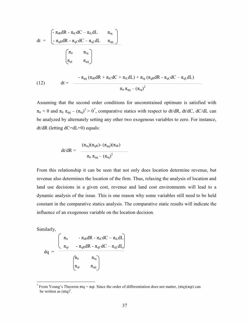
- πqq (πtRdR + πtCdC + πtLdL) + πtq (πqRdR - πqCdC πqLdL)
πtt πqq (πtq)2
Assum er conditions for unconstrained optimum is satisfied with
πtt < 0 comparative statics with respect to dt/dR, dt/dC, dC/dL can
e analyzed by alternately setting any other two exogenous variables to zero. For instance,
(πtq)(πqR)- (πqq)(πtR)
tt qq tq
on of the firm. Thus, relaxing the analysis of location and
nd use decisions in a given cost, revenue and land cost environments will lead to a
eason why some variables still need to be held
is. The comparative static results will indicate the
fluence of an exogenous variable on the location decision.
- πtRdR - πtCdC πtLdL πtq
dL πqq dt = - πqRdR - πqCdC πqL
π π tt tq
qt qq π π
(12) dt =
ing that the second ord
and πtt πqq (πtq)2 > 07,
b
dt/dR (letting dC=dL=0) equals:
dt/dR = π π (π )2
From this relationship it can be seen that not only does location determine revenue, but
revenue also determines the locati
la
dynamic analysis of the issue. This is one r
constant in the comparative st tics a ala n ys
in
Similarly,
πtt - πtRdR - πtCdC πtLdL
πqt - πqRdR - πqCdC πqLdL dq =
π π
π π tt tq
qt qq
37
7 From Youngs Theorem πtq = πqt. Since the order of differentiation does not matter, (πtq)(πqt) can be written as (πtq)2.

- πtt (πqRdR + πqCdC + πqLdL) + πqt (πtRdR + πtCdC + πtLdL)
tt qq tq
generated for dq/dR, dq/dC, and dq/dL. For instance,
e
dq/dL = (πtt)(πqq) (πtq)2
he comparative static results from the consideration of the optimal land size decision and
spect to changes in those exogenous variables.
nd-Use and Location Decisions for Personal
ers)
ith
gard to location and plot size use can be characterized as follows.
(14)
t = the location/distance from a given population center
The co maximize the level of attainable utility arising from a decision
a
t generates its own utility, including scenic values and safe
(13) dq = π π (π )2
Comparative static results can be
dq/dL (by letting dR=dC=0) provid s:
(πqt)(πtL)- (πtt)(πqL) T
exogenous variable of interest can provide relevant information on the sensitivity of
optimal land size considerations with re
2.5.2. Mathematical Consideration of La
Consumption Purposes (Consum
Yet another spatial pressure on the use of land comes from consumers for purposes of
residence and related personal uses, or as usually referred to as direct consumption.
Mathematically, following Alonso, (1964), the economic behavior of consumers w
re
Max U=U(h, q, t)
Where U = Utility
h = a bundle of all other goods and services the consumer may prefer to
consume
q = the quantity of land preferred for direct uses
nsumers goal is to
to consume a given combination of h, q, and t. Location (t) could be viewed as
consumable commodity as i
38

n . h can be viewed as a Hicksian bundle or a comeighborhoods posite good the consumer
ay pr er to c
ity of each that the consumer may prefer to consume cannot
xceed the available resource of the consumer the budget constraint. Mathematically, it
8
price of land at a given location t
q = the quantity of land for private consumptive uses
k muting to a center from location/distance t
ome, what level of h (a
distance
ility within the existing budget
n dU = 0. Totally
n
m ef onsume.
However, the choice of a maximum level of utility by the consumer is limited by a
budget constraint. It can generally be stated that given the utility maximization objective
of the consumer, the budget of the consumer (income) can be fully allocated among
consumption options of h, t and q. From this it can be stated that the price of these
options times the quant
e
can be expressed as:
(15) Y=Phh + P(t)q + Ck (t)
where Y = income
Ph = price of the composite good/commodity bundle
h = a basket of preffered consumption goods/commodity bundle
P(t) = the
C (t) = the cost of com
The decision problem to the consumer here is, given prices and inc
consumption bundle), q (land size to use for private purposes), and t (at what
from the center of activity) will satisfy maximum ut
constraint. The utility function, U=U(h,q,t), is at maximum whe
differe tiating U we get:
(16) dU = (∂U/∂h)dh + (∂U/∂q)dq + (∂U/∂t)dt = 0 Holding t constant at some given distance (dt=0) we have:
8 The setup of the budget constraint implicitly suppresses possible savings. Consequently, it disregards utility associated with savings. This topic is not critically relevant to the present case, however, Y can be
viewed as discretionary income (total income less obligatory payments for example, taxes and savings) for allocation among goods to attain maximum utility associated with that level of resource.
39

dU = (∂U/∂h)dh + (∂U/∂q)dq = 0
(∂U/∂h)dh = (-∂U/∂q)dq
8) - dh/dt = (∂U/∂t)/( ∂U/∂h)
portant information can also be captured by totally differentiating the budget
e in income affects h, q, k and p.
This m unt of h one can afford changes. Similarly, the
amount e amount we can afford to spend on commuting changes
ic k (t)). The price of land also changes as it depends on
here it is located. However, assuming perfect competition in all markets, the prices
Phdh + P(t)dq + [(dCk(t)/dt) + q(dp(t)/dt)]dt = 0
ince the problem deals with a three-dimensional surface, a cross section at a constant Y
cross sectional
(17) - dh/dq = (∂U/∂q)/( ∂U/∂h)
Now holding q constant at some size (dq=0) we have:
dU = (∂U/∂h)dh + (∂U/∂t)dt = 0
(∂U/∂h)dh = (- ∂U/∂t)dt
(1
Im
constraint. From equation 15 we can see that a chang
eans as income changes, the amo
of land preferred and th
(impl itly affecting location since C
w
remain unaffected by a change in income since a given consumer has limited influence
over market prices, as there are many buyers and sellers. Therefore, dY can be expressed
as:
(19) dY=(∂Y/∂h)dh + (∂Y/∂q)dq + (∂Y/∂Ck(t))(∂Ck(t)/∂t)dt + (∂Y/∂p(t))(∂p(t)/∂t)dt= 0 Substituting the relevant partial derivatives from equation 2 we get:
dY = Phdh + P(t)dq +(dCk(t)/dt)dt + q(dp(t)/dt)dt = 0
(20)
S
can be evaluated by holding t and q variables constant separately. The
representation when t is held constant is:
40

Phdh + P(t)dq = 0
h
h
etting t vary and holding q constant, the cross sectional representation yields:
h k + q(dp(t)/dt)]dt = 0
/dt) + q(dp(t)/dt)]dt
q(dp(t)/dt)]/ Ph
- dh/dq = P(t)/ Ph = - dh/dq = (∂U/∂q)/( ∂U/∂h
(23)
- dh/dt = (∂U/∂t)/( ∂U/∂h) = -dh/dt = [(dCk(t)/dt) + q(dp(t)/dt)]/ Ph
(t)/dt) + q(dp(t)/dt)]/ Ph
imization and the budget constraint conditions, the
consumer will optimally decide on the allocation of the budget between h*, q*, and t*.
Equatio ion condition.
f Substitution of land and the
omposite goods should equal their price ratios. Similarly, equation 24 dictates that the
ite
oods, [(dCk(t)/dt) + q(dp(t)/dt)] associated with (∂U/∂t) deserves some explanation.
P dh = - P(t)dq
(21) - dh/dq = P(t)/ P
L
P dh + [(dC (t)/dt)
Phdh = - [(dCk(t)
(22) -dh/dt = [(dCk(t)/dt) +
Equating equations 17 and 21:
P(t)/ Ph = (∂U/∂q)/( ∂U/∂h)
Equating equations 18 and 22:
(24) (∂U/∂t)/( ∂U/∂h) = [(dCk
Therefore, solving for the utility max
ns 23 and 24 hold key information about the utility maximizat
Equation 23 dictates that at optimal the Marginal Rate o
c
Marginal Rate of Substitution between distance and the bundle of goods should equal
their price/marginal cost ratio. Though Ph is easily understood as price of the compos
g
(dCk(t)/dt) captures the change in commuting cost with a change in distance and
q(dp(t)/dt) captures a resulting change in land prices with a change in distance.
41

From equation 24, we can extract one more vital piece of information. One can easily
argue that Ph , ∂U/∂h, q ≥ 0. Prices and quantities are typically positive.9 Utility increases
as a person gets more and more consumable commodities hence ∂U/∂h > 0. However,
∂U/∂t < 0 since the further one is located from the center of activity, the more discomfort
nd disutility may arise through spending more time and resources on commuting.
bles
ill not alter the microeconomic foundation if amenity values are translated in the market
Lagrangian expression and solving for first order conditions yields:
a
dCk(t)/dt>0 as commuting costs increase with distance. Therefore, it is possible to isolate
dp(t)/dt < 0 for the whole relationship to hold. Thus, it can be concluded that the
individual will commute so long as |dp(t)/dt| ≥ dCk(t)/dt, i.e, so long as the savings in
land associated with distance from a center exceeds the marginal cost of transportation to
the center. The person avoids locations where dCk(t)/dt > |dp(t)/dt|, ceteris paribus.
An interesting argument can be raised that though the commuting cost is greater than the
savings from land, such locations may be preferred if they have high quality natural
amenities that are not reflected in the market. In this case, it is assumed here that all other
variables that interact in the system are assumed constant. The inclusion of such varia
w
or if such considerations directly enter the utility function of individuals.
Comparative Static Considerations
As in the case of firms, similar comparative statics analysis can be developed for the
utility maximization problem. Setting up and solving the system for first order conditions
yields:
(25) Max U=U(h, q, t)
s.t. Y=Phh + P(t)q + Ck (t)
Setting up the
9 Under rare analytical circumstances prices can assume negative values when resources are received with a
per unit payment for receiving them. Poultry litter could be an example. Litter can be used as an input in a farm while the chicken producer may pay per unit price for disposing his litter off his plant to the farm. Hence the farmer can get the litter at a negative price. This discussion is irrelevant for most economic analysis since it is a rare economic phenomenon.
42
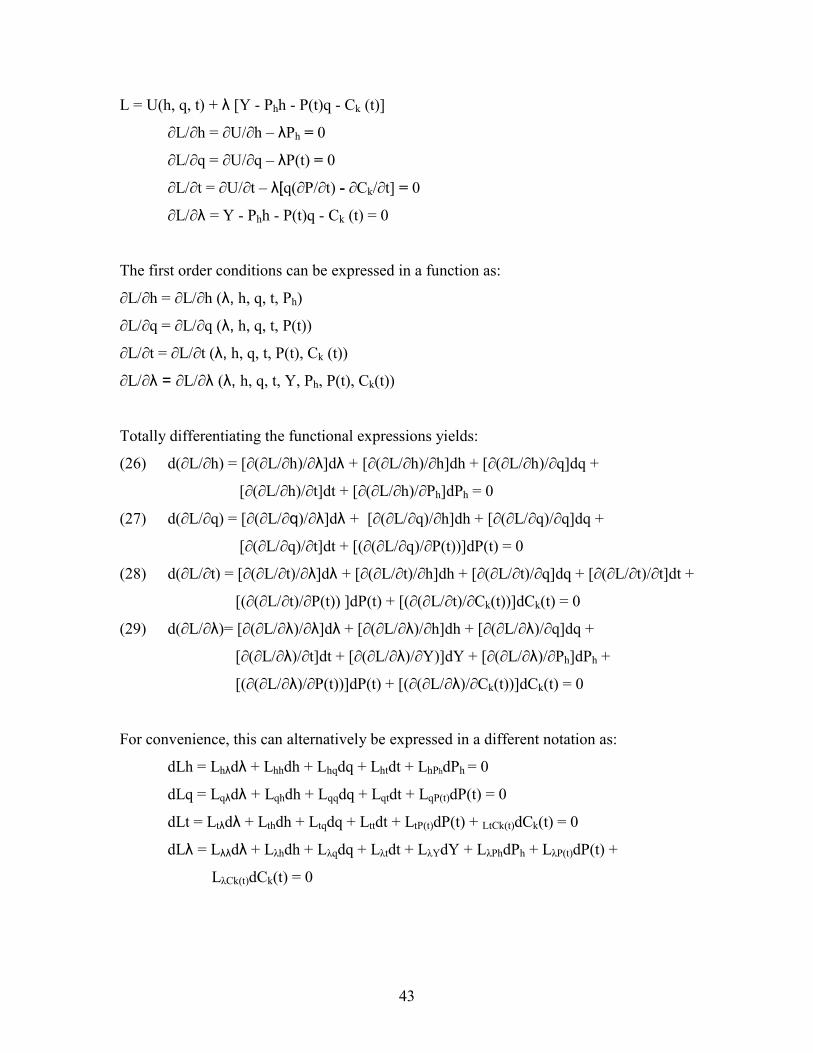
L = U(h, q, t) + λ [Y - Phh - P(t)q - Ck (t)]
L/∂q = ∂U/∂q λP(t) = 0
L/∂λ = Y - Phh - P(t)q - Ck (t) = 0
The fir expressed in a function as:
∂L/∂h =
L/∂q =
L/∂t =
L/∂λ = ∂L/∂λ (λ, h, q, t, Y, Ph, P(t), Ck(t))
ctional expressions yields:
]dλ + [∂(∂L/∂h)/∂h]dh + [∂(∂L/∂h)/∂q]dq +
∂(∂L/∂h)/∂Ph]dPh = 0
/∂q)/∂h]dh + [∂(∂L/∂q)/∂q]dq +
[∂(∂L/∂q)/∂t]dt + [(∂(∂L/∂q)/∂P(t))]dP(t) = 0
(∂L/∂t)/∂q]dq + [∂(∂L/∂t)/∂t]dt +
L/∂λ)/∂q]dq +
k(t) = 0
n as:
dLλ = Lλλdλ + Lλhdh + Lλqdq + Lλtdt + LλYdY + LλPhdPh + LλP(t)dP(t) +
∂L/∂h = ∂U/∂h λPh = 0
∂
∂L/∂t = ∂U/∂t λ[q(∂P/∂t) - ∂Ck/∂t] = 0
∂
st order conditions can be
∂L/∂h (λ, h, q, t, Ph)
∂ ∂L/∂q (λ, h, q, t, P(t))
∂ ∂L/∂t (λ, h, q, t, P(t), Ck (t))
∂
Totally differentiating the fun
(26) d(∂L/∂h) = [∂(∂L/∂h)/∂λ
[∂(∂L/∂h)/∂t]dt + [
(27) d(∂L/∂q) = [∂(∂L/∂q)/∂λ]dλ + [∂(∂L
(28) d(∂L/∂t) = [∂(∂L/∂t)/∂λ]dλ + [∂(∂L/∂t)/∂h]dh + [∂
[(∂(∂L/∂t)/∂P(t)) ]dP(t) + [(∂(∂L/∂t)/∂Ck(t))]dCk(t) = 0
(29) d(∂L/∂λ)= [∂(∂L/∂λ)/∂λ]dλ + [∂(∂L/∂λ)/∂h]dh + [∂(∂
[∂(∂L/∂λ)/∂t]dt + [∂(∂L/∂λ)/∂Y)]dY + [∂(∂L/∂λ)/∂Ph]dPh +
[(∂(∂L/∂λ)/∂P(t))]dP(t) + [(∂(∂L/∂λ)/∂Ck(t))]dC
For convenience, this can alternatively be expressed in a different notatio
dLh = Lhλdλ + Lhhdh + Lhqdq + Lhtdt + LhPhdPh = 0
dLq = Lqλdλ + Lqhdh + Lqqdq + Lqtdt + LqP(t)dP(t) = 0
dLt = Ltλdλ + Lthdh + Ltqdq + Lttdt + LtP(t)dP(t) + LtCk(t)dCk(t) = 0
LλCk(t)dCk(t) = 0
43

Rearran
(30)
Lqtdt = -LqP(t)dP(t)
2) Ltλdλ + Lthdh + Ltqdq + Lttdt = -LtP(t)dP(t) - (LtCk(t)dCk(t)
3) Lλλdλ + Lλhdh + Lλqdq + Lλtdt = -LλP(t)dP(t) - LλCk(t)dCk(t) - LλYdY - LλPhd Ph
Rule to the
h dh/dy, dh/ Ph etc and any
Hessian matrix is negative
ular economic agent. The final spatial feature, thus, will be determined by the
ynamics of economic interests and competition.
ging:
Lhλdλ +Lhhdh + Lhqdq + Lhtdt = -LhPhdPh
(31) Lqλdλ + Lqhdh + Lqqdq +
(3
(3
Lλλ Lλh Lλq Lλt dλ -LλP(t)dP(t) - LλCk(t)dCk(t) - LλYdY - LλPhdPh
LhPhdPh Lhλ Lhh Lhq Lht dh = -
Lqλ Lqh Lqq Lqt dq -LqP(t)dP(t)
Ltλ Lth Ltq Ltt dt -LtP(t)dP(t) - LtCk(t)dCk(t)
Solutions for dλ, dh, dq and dt can be generated by applying Cramers
matrices. Comparative statics can be carried out on d /dp,
other relationship of interest provided that the bordered
definite.
To conclude, economic agents operate to maximize gains given different constraints. The
allocation of land at a given location thus depends on which economic agent promises the
payment of the highest bid rent depending on the relative benefit of the location (land) to
any partic
d
44

CHAPTER III
MODELING AGRICULTURAL LAND CONVERSION IN A
REGIONAL GROWTH FRAMEWORK
3.1. GENERAL MODELING OVERVIEW
The a ong
different competing economic agents have been a concern for different disciplines.
Numerous analyses have focused on this challenging issue from quite diverse perspective
and approaches.
present topic of interest, land is one consumable good (for housing,
creation, open space, ) that provides utility to consumers. Similarly, producers
and to different uses can be captured accordingly.
nalysis and modeling of land use across different sectors of an economy and am
As outlined in the previous chapter, economic agents behave in maximizing behavioral
interests. Consumers generally maximize utility given the consumption of different goods
and services available in their endowment basket, which is subject to the individuals
income. For the
re
generally behave to maximize profits by efficiently utilizing factors to supply goods
and/or services. Land, as a significant factor input, determines the cost as well as the
revenue structure of business enterprises. Hence, an efficient location decision, as well as
efficient land size determination are criteria in the profit maximization endeavor. The
competition for land results in spatial frictions that are evident across a given landscape
through time.
Understanding the underlying economic motives of economic agents and capturing
behavioral friction across space is a complex undertaking and a critical requirement in the
modeling process of land use. A change in economic activity across space and gradual
conversion of l
Generally, the competing demands for a fixed physical supply of land for different uses
can be treated as a special case of the overall determination of the flow of resources
45

46
(factors), products and services in an economy. Broadly viewed, this process can be
represented by the circular flow chart in figure 7.
Fig. 7. Interdependent Circular Flow Chart
Traditionally, consumers (households) are treated as suppliers of factors (labor; capital)
to producers through the factor market and earn factor compensation and income.
Producers use these factor supplies in the production process to supply goods and
services to consumers through the product market to generate profits. Government
operates as providing the required market infrastructure, legal settings, and policies to
coordinate producers and consumers. This emphasizes a unidirectional flow of resources
and products across the economy.
However, as indicated in figure 7, the flow of resources is multidirectional involving use
friction. Consumers (households) do not only supply factors but can also demand them
from the factor market and producers not only demand factor inputs, they can decide to
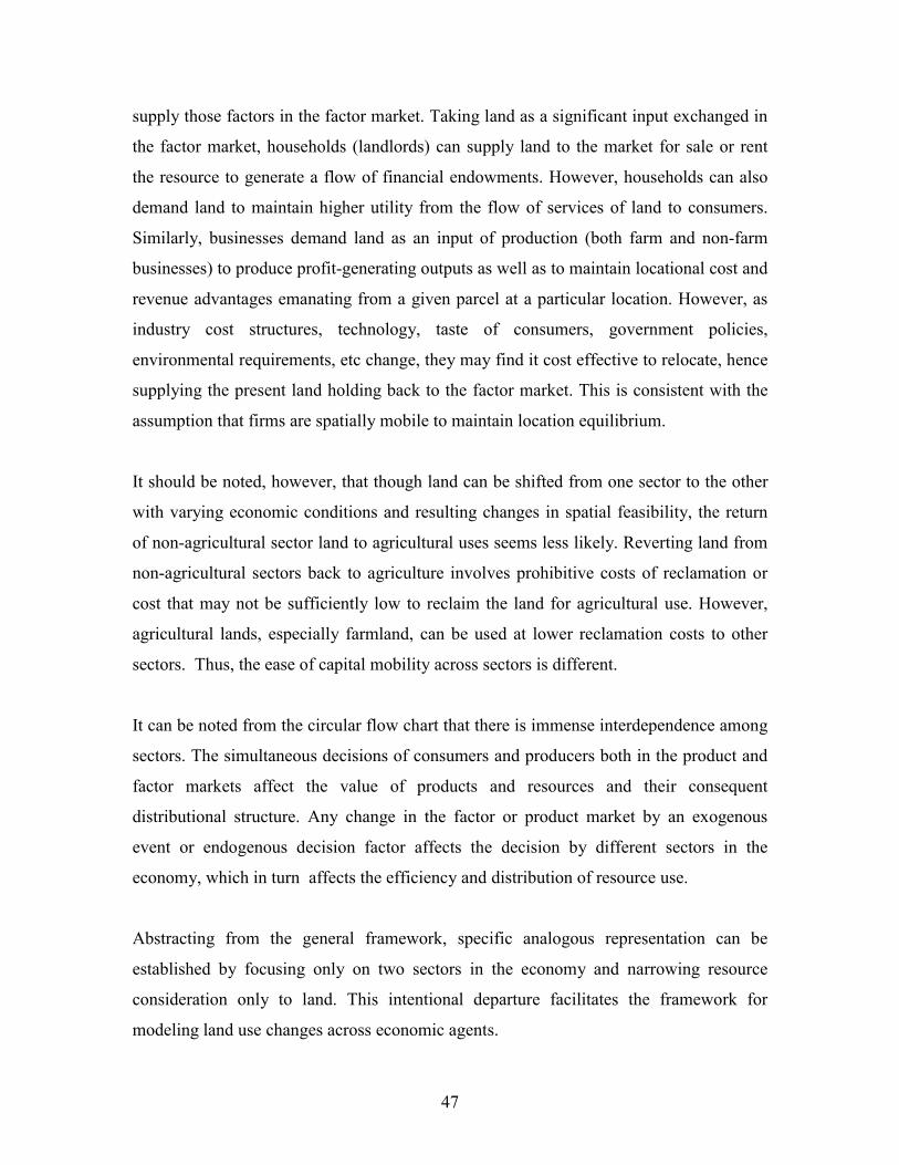
supply those factors in the factor market. Taking land as a significant input exchanged in
the factor market, households (landlords) can supply land to the market for sale or rent
e resource to generate a flow of financial endowments. However, households can also
se. However,
gricultural lands, especially farmland, can be used at lower reclamation costs to other
sectors in the
conomy, which in turn affects the efficiency and distribution of resource use.
modeling land use changes across economic agents.
th
demand land to maintain higher utility from the flow of services of land to consumers.
Similarly, businesses demand land as an input of production (both farm and non-farm
businesses) to produce profit-generating outputs as well as to maintain locational cost and
revenue advantages emanating from a given parcel at a particular location. However, as
industry cost structures, technology, taste of consumers, government policies,
environmental requirements, etc change, they may find it cost effective to relocate, hence
supplying the present land holding back to the factor market. This is consistent with the
assumption that firms are spatially mobile to maintain location equilibrium.
It should be noted, however, that though land can be shifted from one sector to the other
with varying economic conditions and resulting changes in spatial feasibility, the return
of non-agricultural sector land to agricultural uses seems less likely. Reverting land from
non-agricultural sectors back to agriculture involves prohibitive costs of reclamation or
cost that may not be sufficiently low to reclaim the land for agricultural u
a
sectors. Thus, the ease of capital mobility across sectors is different.
It can be noted from the circular flow chart that there is immense interdependence among
sectors. The simultaneous decisions of consumers and producers both in the product and
factor markets affect the value of products and resources and their consequent
distributional structure. Any change in the factor or product market by an exogenous
event or endogenous decision factor affects the decision by different
e
Abstracting from the general framework, specific analogous representation can be
established by focusing only on two sectors in the economy and narrowing resource
consideration only to land. This intentional departure facilitates the framework for
47

48
Suburban and rural land, as indicated earlier, can be demanded for direct use by
consumers and by agricultural and non-agricultural producers. Consumers demand for
land can be motivated by a number of factors. As indicated in figure 8, consumers
(households) tend to demand more sub-urban and rural land as population pressure and
urban congestion intensifies and as the quality of life including natural amenities tend to
be valued higher by households for housing and recreational purposes. Households can
also be attracted to suburban areas for employment as there are growing small business
enterprises across the urban fringe and emerging rural economies.
The demand of rural and suburban land for agricultural land purposes is motivated by
fertility and location factors affecting the profit of farmers, the agglomeration of farms in
the farm environment, and the farming tradition maintained for generations. However,
with intensified competition over suburban land on the one hand and lesser per acre
return of agricultural enterprises on the other has led to the conversion of land to other
non-agricultural uses. This implies that the agricultural sector is not only a source of
demand for land, but is also a net supplier of rural land for other competing uses.
Fig. 8. Reduced Form Specialized Two Sectors Circular Flow Chart.
DemandLand fertility Closeness to markets Farm agglomeration Locational cost savingFarming tradition etc
Population growth in cities Urban Congestion Sub-urban natural amenities Location convenience Residential preferences Employment
PRODUCERS: AGRICULTURAL
PRODUCERS: NON-AGRI.
CONSUMERS
Demand Sub-Urban and Rural Land
Competition, Value, and Use
Transport cost savings Population growth & market centers Agglomeration economies Land cost saving Locational labor cost savings etc
Natural amenity endowment Positive surrounding externalities Fertility Locational endowment Physical characteristics etc
Further Suburbanization
Relative gravity and use conversion Relative gravity and use conversion
Relative gravity and use conversion
Qua
litie
s
Demand
Supply
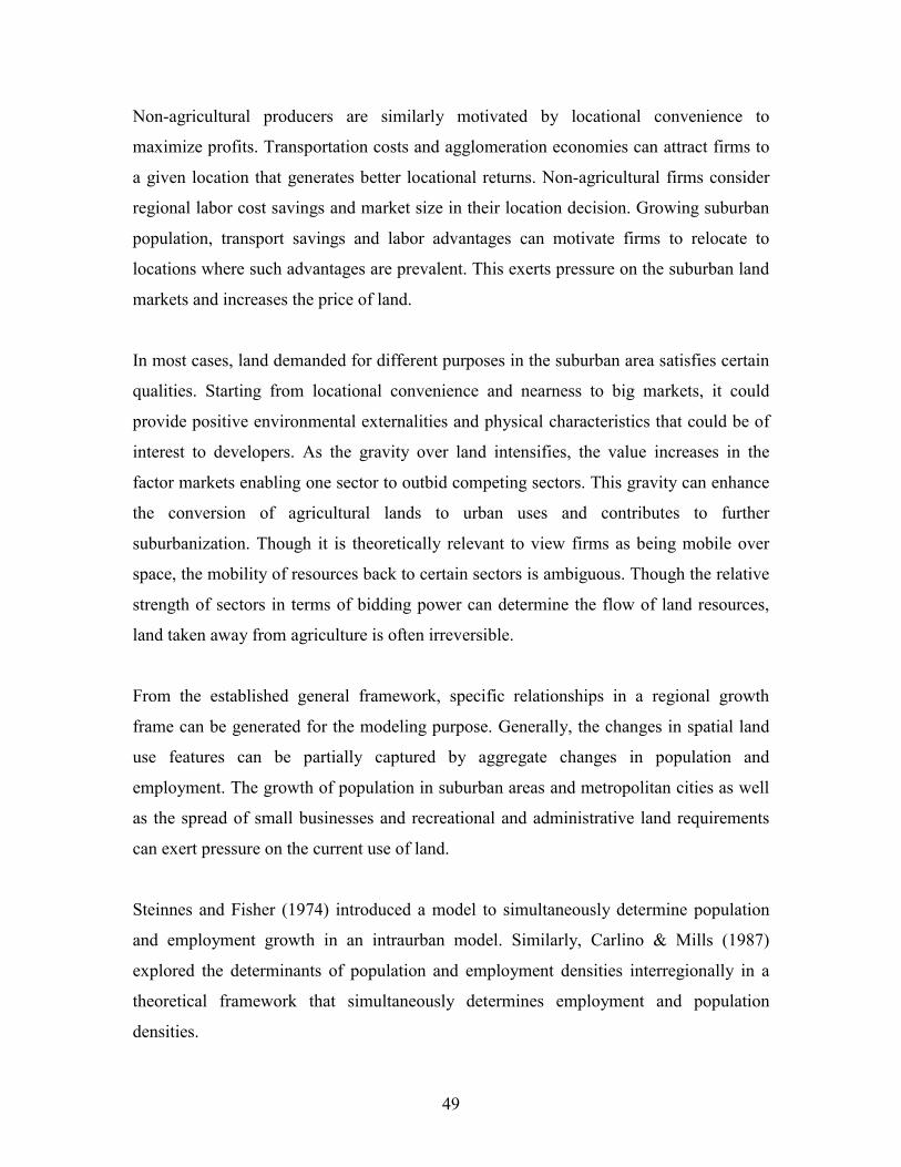
Non-agricultural producers are similarly motivated by locational convenience to
maximize profits. Transportation costs and agglomeration economies can attract firms to
a given location that generates better locational returns. Non-agricultural firms consider
regional labor cost savings and market size in their location decision. Growing suburban
population, transport savings and labor advantages can motivate firms to relocate to
locations where such advantages are prevalent. This exerts pressure on the suburban land
markets and increases the price of land.
In most cases, land demanded for different purposes in the suburban area satisfies certain
qualities. Starting from locational convenience and nearness to big markets, it could
provide positive environmental externalities and physical characteristics that could be of
interest to developers. As the gravity over land intensifies, the value increases in the
factor markets enabling one sector to outbid competing sectors. This gravity can enhance
the conversion of agricultural lands to urban uses and contributes to further
burbanization. Though it is theoretically relevant to view firms as being mobile over
densities.
su
space, the mobility of resources back to certain sectors is ambiguous. Though the relative
strength of sectors in terms of bidding power can determine the flow of land resources,
land taken away from agriculture is often irreversible.
From the established general framework, specific relationships in a regional growth
frame can be generated for the modeling purpose. Generally, the changes in spatial land
use features can be partially captured by aggregate changes in population and
employment. The growth of population in suburban areas and metropolitan cities as well
as the spread of small businesses and recreational and administrative land requirements
can exert pressure on the current use of land.
Steinnes and Fisher (1974) introduced a model to simultaneously determine population
and employment growth in an intraurban model. Similarly, Carlino & Mills (1987)
explored the determinants of population and employment densities interregionally in a
theoretical framework that simultaneously determines employment and population
49

In the Carlino-Mills model, a general equilibrium approach addresses that both
households and producers are geographically mobile. Consumers maximize utility, which
epends on purchased goods and services, on locations relative to work places, and on
s. They assume that firms and households adjust to disequilibrium by
ies Act through the
stimation of the relationship between the number of listed species in a county and
d
spatially varying nonmarket amenities. A conventional budget constraint equates income
to the sum of spending on goods and services. Profit-maximizing firms production costs
vary by location because of regional comparative advantages, including transport cost
differentials, regional variation in labor supply, agglomeration economies, and state and
local taxe
distributed-lag adjustment equations. In such a model, equilibrium population and
employment are simultaneously determined. (Carlino & Mills, 1987).
A similar approach is also followed by Deller, et al., (2001) to investigate the nature and
extent of economic structural change in the United States with a particular focus on the
role of non-market amenity attributes. Based on free migration assumptions they identify
the effects of amenity-based attributes on regional economic growth.
Following a similar modeling technique, Duffy-Deno, (1997) employed the regional
growth model to analyze the economic effects of the Endangered Spec
e
county employment growth during the 1980s. In this disequilibrium model of regional
growth, where households and firms are assumed to be geographically mobile, a log-
linear distributed adjustment lag model is introduced for population and employment
interactions.
Following the spirit of the Carlino-Mills model, this research work employs the regional
growth model to investigate the simultaneous interaction of employment, population, and
agricultural lands to capture the impact of growth on agricultural land conversion in West
Virginia.
50

3.2. EMPIRICAL MODEL
s interaction of population, employment, agricultural land and other relevant
ariables of interest would provide a picture of land conversion processes in the study
ssumed that consumers maximize utility by the consumption of a vector of goods
nd services. Consumers consume goods and services as well as location and nonmarket
migrate until utilities are equalized at different alternative locations.
is also assumed that firms and households adjust to disequilibrium by distributed-lag
be
imultaneously determined in such a general equilibrium model, along with population
Regional growth models are one approach to capture the effects of growth factors on the
conversion of agricultural lands. As specified in the previous section, employment and
population growth changes can explain the pressure on resources. Capturing the
simultaneou
v
area.
The empirical model is specified following the Carlino-Mills general equilibrium model
where firms and households adjust to disequilibrium by distributed-lag adjustment
equations.
It is a
a
amenities to maximize their utility. Consumers are mobile over locations that maximize
utility. The consumption of the vector of consumer choices is limited by income (budget).
Households
Producers are assumed to maximize profit from the production of goods and services.
Firms select locations to capture locational cost and revenue advantages, minimize the
cost of transportation, benefit from agglomeration, and regional labor supply differences.
Firms enter and leave regions until competitive profits are equalized across regions.
It
adjustment equations. In a general equilibrium framework, population and employment
are affected not only by each other, but also by a variety of other variables that affect
numbers of jobs consistent with competitive profit rates and number of people consistent
with equalized utility levels among places. In principle, many such variables might
s
and employment (Carlino & Mills, 1987).
51

Thus, following the assumptions and simultaneous determination process, the general
model can be specified as:
(1) E* = ΨEP + ΦEΩ
(2) P* = Ψ
E
PE + ΦPΩP
here E is total employment, P is total population, ΩE and ΩP are vectors of exogenous
uilibrium levels of employment and population depend on the
ctu of employment and pop f other factors belonging to
the E and ΩP.
E = Et-1 + E(E* - Et-1)
(4) P = Pt-1 + P(P* - Pt-1)
Where and are speed-of-adjustment coefficients with 0 ≤ ≤ 1, and t-1 is a one
period lag. This indicates that current employment and population are dependent on one
period lagged levels of population and employment and on the change between
equ um values and one lagged d t speed-of-adjustment values
of P. Substituting E* and P* a ves:
E
(5) E = E ΨEP + E ΦEΩ + (1-E) Et-1
)
W
variables that affect employment (E) and population (P), and * indicates equilibrium
levels of E and P. Hence, eq
a al level ulation and on a vector o
sets Ω
Population and employment are likely to adjust to equilibrium values with substantial
lags (Mills & Price, 1984). Thus a distributed lag adjustment equation can be introduced
as:
(3)
E P E, P
ilibri period values adjuste a
E and in equ tions 3 and 4 gi
E = Et-1 + E(ΨEP + ΦEΩ - Et-1)
P = Pt-1 + P(ΨPE + ΦPΩP - Pt-1)
Rearranging terms gives:
E
(6 P = PΨPE + P ΦPΩP + (1-P) Pt-1
52
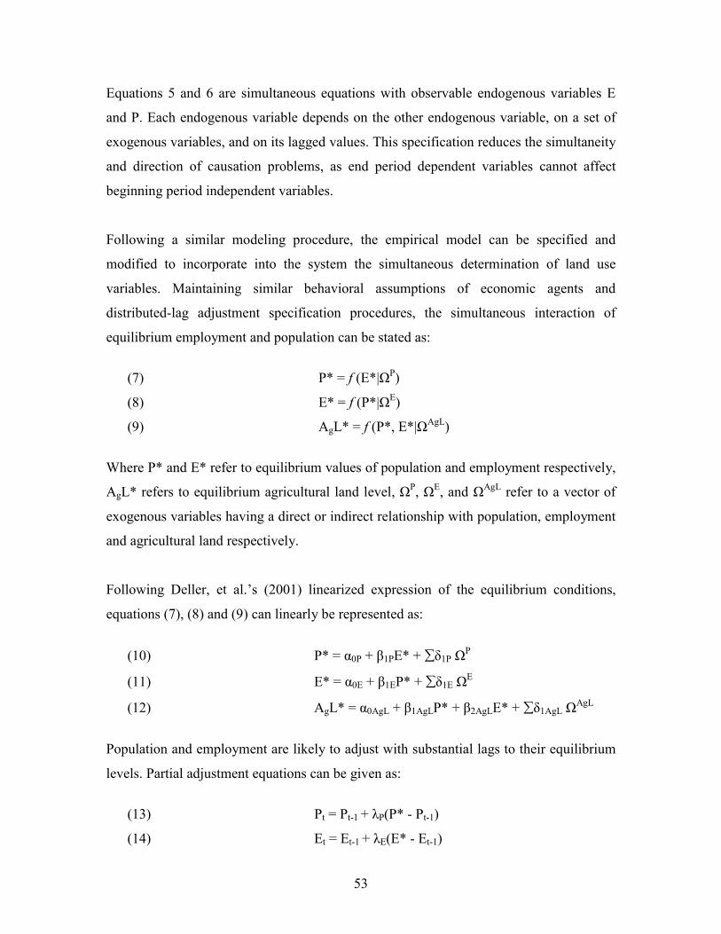
Equations 5 and 6 are simultaneou ogenous variables E
nd P. Each endogenous variable depends on the other endogenous variable, on a set of
n its lagged values. This specification reduces the simultaneity
nd direction of causation problems, as end period dependent variables cannot affect
beg period independent variab
ollowing a similar modeling procedure, the empirical model can be specified and
modified to incorporate into the system the simultaneous determination of land use
variables. Maintaining similar behavioral assumptions of economic agents and
distributed-lag adjustment specification procedures, the simultaneous interaction of
equilibrium employment and population can be stated as:
(7) P* = f (E*|ΩP)
, and ΩAgL refer to a vector of
xogenous variables having a direct or indirect relationship with population, employment
and ultural land respectively.
Fol o the equilibrium conditions,
quations (7), (8) and (9) can linearly be represented as:
AgL* = α0AgL + β1AgLP* + β2AgLE* + δ1AgL ΩAgL
s equations with observable end
a
exogenous variables, and o
a
inning les.
F
(8) E* = f (P*|ΩE)
(9) AgL* = f (P*, E*|ΩAgL)
Where P* and E* refer to equilibrium values of population and employment respectively,
AgL* refers to equilibrium agricultural land level, ΩP, ΩE
e
agric
lowing Deller, et al.s (2001) linearized expression f
e
(10) P* = α0P + β1PE* + δ1P ΩP
(11) E* = α0E + β1EP* + δ1E ΩE
(12)
Population and employment are likely to adjust with substantial lags to their equilibrium
levels. Partial adjustment equations can be given as:
(13) Pt = Pt-1 + λP(P* - Pt-1)
(14) Et = Et-1 + λE(E* - Et-1)
53

whe nt,
t-1 and Et-1 are initial conditions of population and employment.
P Pt-1)
Et-1)
nd employment levels
spectively.
ubstituting the linear expressions of P* and E* (equations 10 and 11) into equations (15)
and (16) results in:
(17) ∆P = Pt - Pt-1 = λP(α0P + β1PE* + δ1P ΩP - Pt-1)
t t-1 E 0E 1E 1E t-1
earranging and substituting the expressions we have:
∆P = α0P + β1PPt-1 + β2PEt-1 + β3P ∆E + δ1P ΩP
(20) ∆E = α0E + β1EPt-1 + β2EEt-1 + β3E ∆P + δ1E ΩE
Not the speed-of-adjustment λ b d f ent
arameters α, β, and δ. (Deller, et al., 2001).
corporating the change in agricultural land in combination with population and
em ent changes, the system of
P
β3E ∆P + δ1E ΩE
(23) ∆AgL = α0AgL + β1AgLPt-1 + β2AgLEt-1 + β3AgL∆P+ β3AgL∆E+ δ1AgLΩ AgL
re λP and λE are speed-of-adjustment coefficients for population and employme
P
Rearranging terms:
(15) ∆P = Pt - Pt-1 = λ (P* -
(16) ∆E = Et - Et-1 = λE(E* -
where ∆P and ∆E are change in county level population a
re
S
(18) ∆E = E - E = λ (α + β P* + δ ΩE - E )
R
(19)
e that coefficient ( ) is em edde in the linear coe fici
p
In
ploym equations growth model can be specified as:
(21) ∆P = α0P + β1PPt-1 + β2PEt-1 + β3P ∆E + δ1P Ω
(22) ∆E = α0E + β1EPt-1 + β2EEt-1 +
54
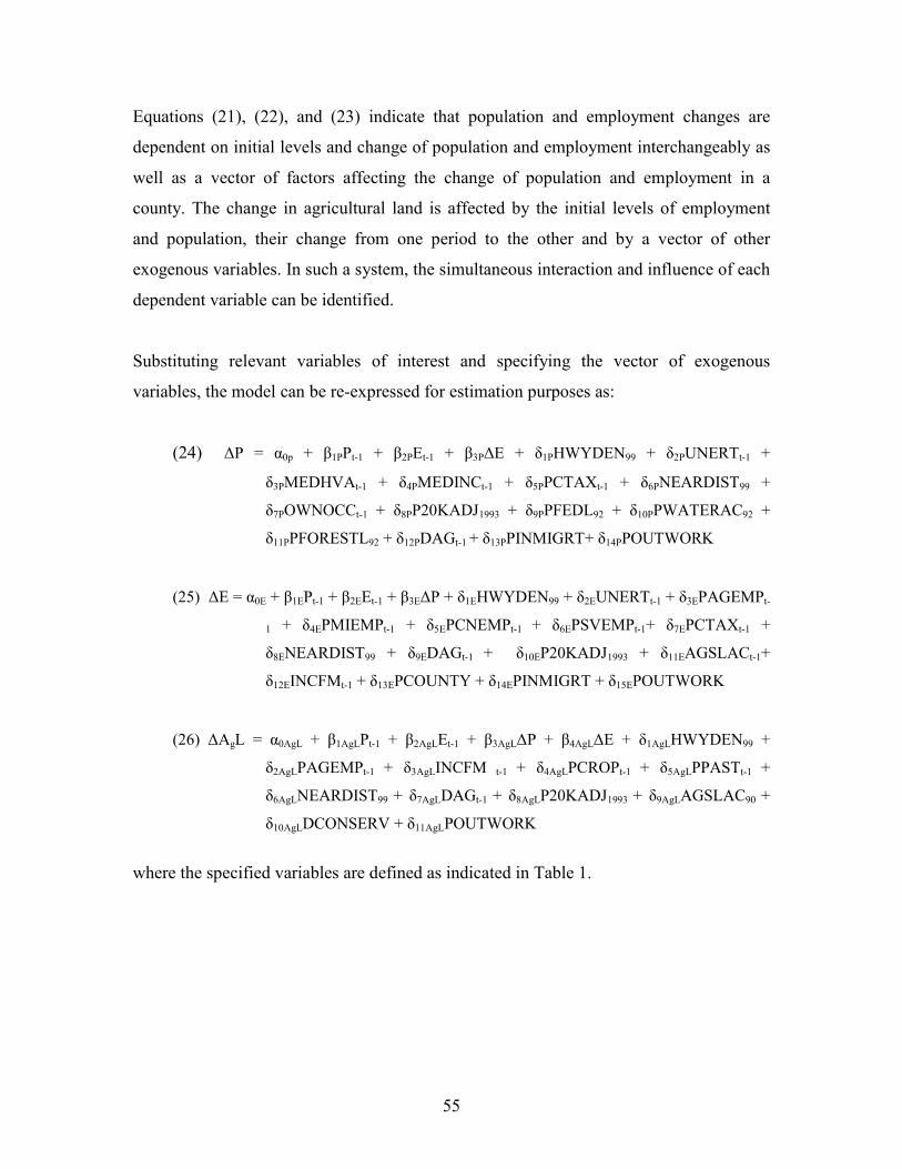
Equations (21), (22), and (23) indicate that population and employment changes are
dependent on initial levels and change of population and employment interchangeably as
ell as a vector of factors affecting the change of population and employment in a
cou he cha al levels of employment
and lation, d by a vector of other
exo s varia h a ch
ependent variable can be identified.
8PP20KADJ1993 + δ9PPFEDL92 + δ10PPWATERAC92 +
δ11PPFORESTL92 + δ12PDAGt-1 + δ13PPINMIGRT+ δ14PPOUTWORK
RTt-1 + δ3EPAGEMPt-
1 + δ4EPMIEMPt-1 + δ5EPCNEMPt-1 + δ6EPSVEMPt-1+ δ7EPCTAXt-1 +
T D E
2
(26) ∆AgL = 0 2 EN99 +
δ2AgLPAGEMPt-1 + δ3AgLINCFM t-1 + δ4AgLPCROPt-1 + δ5AgLPPASTt-1 +
NE I 9 9
C L RK
where the specifie
w
nty. T nge in agricultural land is affected by the initi
popu their change from one period to the other an
genou bles. In suc system, the simultaneous interaction and influence of ea
d
Substituting relevant variables of interest and specifying the vector of exogenous
variables, the model can be re-expressed for estimation purposes as:
(24) ∆P = α0p + β1PPt-1 + β2PEt-1 + β3P∆E + δ1PHWYDEN99 + δ2PUNERTt-1 +
δ3PMEDHVAt-1 + δ4PMEDINCt-1 + δ5PPCTAXt-1 + δ6PNEARDIST99 +
δ7POWNOCCt-1 + δ
(25) ∆E = α0E + β1EPt-1 + β2EEt-1 + β3E∆P + δ1EHWYDEN99 + δ2EUNE
δ8ENEARDIS 99 + δ9E AGt-1 + δ10EP20KADJ1993 + δ11 AGSLACt-1+
δ1 EINCFMt-1 + δ13EPCOUNTY + δ14EPINMIGRT + δ15EPOUTWORK
α AgL + β1AgLPt-1 + β AgLEt-1 + β3AgL∆P + β4AgL∆E + δ1AgLHWYD
δ6AgL ARD ST 9 + δ7AgLDAGt-1 + δ8AgLP20KADJ1993 + δ AgLAGSLAC90 +
δ10AgLD ONSERV + δ11Ag POUTWO
d variables are defined as indicated in Table 1.
55
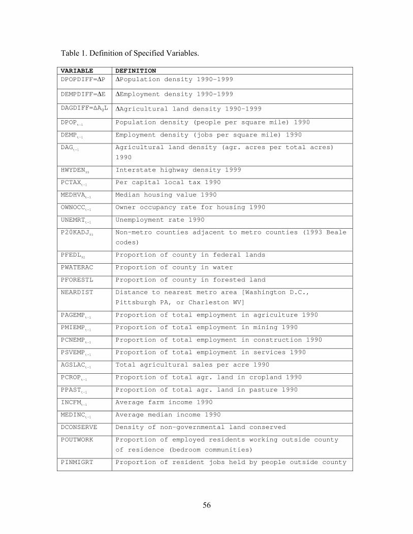
Table 1. Definition of Specified Variables.
ARIABLE DEFINITION VDPOPDIFF=P Population density 1990-1999
DEMPDIFF=E Employment density 1990-1999
DAGDIFF=∆AgL Agricultural land density 1990-1999
DPOPt-1 Population density (people per square mile) 1990
DEMPt-1 Employment density (jobs per square mile) 1990
DAGt-1 Agricultural land density (agr. acres per total acres)
1990
HWYDEN99 Interstate highway density 1999
t-1
t-1
OWNOCC
codes)
Pittsburgh PA, or Charleston WV]
PAGEMPt-1 Proportion of total employment in agriculture 1990
PMIEMPt-1 Proportion of total employment in mining 1990
P
t-1
t-1
PCTAX Per capital local tax 1990
MEDHVA Median housing value 1990
t-1 Owner occupancy rate for housing 1990
UNEMRTt-1 Unemployment rate 1990
P20KADJ93 Non-metro counties adjacent to metro counties (1993 Beale
PFEDL92 Proportion of county in federal lands
PWATERAC Proportion of county in water
PFORESTL Proportion of county in forested land
NEARDIST Distance to nearest metro area [Washington D.C.,
PCNEMPt-1 Proportion of total employment in construction 1990
PSVEM t-1 Proportion of total employment in services 1990
AGSLACt-1 Total agricultural sales per acre 1990
PCROPt-1 Proportion of total agr. land in cropland 1990
PPASTt-1 Proportion of total agr. land in pasture 1990
INCFM Average farm income 1990
MEDINC Average median income 1990
DCONSERVE Density of non-governmental land conserved
POUTWORK Proportion of employed residents working outside county
of residence (bedroom communities)
PINMIGRT Proportion of resident jobs held by people outside county
56
The model speci erent variables
on the bles. The change in population density is
simultaneously determined by changes in employment and initial population conditions
as generated from the interaction growth model. The change in employment density,
however, is also cified in equation (24).
edian housing value, percentage of houses that are owner occupied, and median
median household income and a reduction in property values expand the
tility maximizing goods bundle, including housing and recreational site choices. This
lation equation and directly through its
ffect on crime rates and safety affecting individual location decisions for housing and
fication identifies direct and indirect relationships of diff
of interest change in the endogenous varia
affected by a vector of other variables as spe
Highway density, nearest distance, and adjacency to urbanized areas variables try to
capture the direct effect of accessibility on population changes. It is expected that the
more accessible a county is, the more (higher) the population density change is in the
location.
M
household income in the sample counties can also be thought of as directly influencing
demographic changes. These variables try to capture population changes derived from
housing and property values in spatial location decisions. It can be argued that an
increase in
u
tends to positively influence population growth.
Per capita tax rates and unemployment are also specified to capture their direct influence
on population. Labor mobility attributes in terms of in-migrating and out-migrating labor
is also introduced. Generally, a higher unemployment rate can reduce population in two
ways; indirectly through reducing people coming to a specific location in search of job
(employment effect) captured by =E in the popu
e
other purposes in that specific location. Generally, the effect of per capita tax on
population could be viewed as negatively related. Those counties with higher per capita
taxes might see people out-migrating to other locations of light fiscal burden or vice
versa. However, it can also be argued that people can also prefer high per capita tax rates
if the area is less populated and has the natural amenities intact than places with high
57

population and congestion and less fiscal burdens. The sign has to be empirically
determined to conclude on both possibilities.
Finally, the listed agricultural variables are related with population changes through the
provision of natural amenities, federal land preservation, and intensity of the agricultural
activity that have a direct bearing on property values and employment opportunities that
directly and indirectly affect population changes.
ted. Extension of highway infrastructure makes the temporary in-
igration of labor and effort supply decisions of distant labor easier. These have a direct
r instance, a growing service industry can attract
mployment from other relatively less paying sectors. This can lead to employment cuts
Similarly, employment density changes are affected by initial employment conditions as
well as change in population for the study period as determined in the simultaneous
equation system. A vector of other relevant variables also directly interacts with
employment growth.
Again, highway densities, distance from metropolitan or urban areas and adjacency to
urbanized areas capture the effects of accessibility on employment changes. Generally,
the more accessible or exposed a county or specific region is, increasing employment
growth can be expec
m
bearing on employment changes.
The decomposition of employment into different sectors identifies the influence of each
employment sector on the overall employment change in West Virginia. Interrelationship
of sectors should carefully be noted to capture the impact of employment change of one
on the overall employment. Fo
e
by other employers to raise the wage and salary. Similarly, the effects of these different
sectors are in part reflected in their overall mobility. For example, the services sector may
be much more mobile than the other sectors. The construction sector typically expands
and contracts based on the demand for their products. Resource-dependent sectors
(agriculture, mining) have limited mobility, as they require location-specific inputs (land,
minerals) in their production processes. Though the actual impact can separately be
58
studied in an impact analysis framework, the interrelationship of different employment
sectors and their influence on overall employment is recognized.
The direct relationship between per capita taxes and unemployment rate with
employment growth is analogous with the effect on population. Higher tax structures can
discourage new businesses and can motivate relocation of businesses and employees to
reduce tax burdens. Analogously, counties with tax incentives can attract more new
usinesses. Hence, the level of imposed tax is generally inversely related with
riculture in retaining its land use as measured by its profitability
nd use of land. Not only is the agricultural sector important for farm employment
employment and population densities will indirectly influence the change (conversion) of
b
employment creation. However, consideration of other factors of positive importance to
businesses and households can offset the negative impact of higher taxes and induce them
to move to areas of high fiscal burden if savings from other attributes of the area are
greater. Higher unemployment rates can also directly affect employment growth trends.
High unemployment regions attract lesser in-migrating laborers as compared to regions
with boosting employment opportunities and high employment growth. This regional
unemployment rate differential can affect and explain some portion of the change in total
employment variations.
Another source of change in employment densities arises from the agricultural sector.
Agricultural sales volume, average farm income (agricultural sales plus all transfer
payments), and agricultural land density measures are specified to capture the
competitive ability of ag
a
opportunities and off-farm employment opportunities through agricultural sectors
backward and forward linkages with other sectors, a decline in agricultural land density
and the shrinking of the agricultural sector will result in a direct cut of farm employment
opportunities as well as related off-farm employment. This directly and indirectly affects
the change in employment density.
Finally, much research focus is placed on the change in agricultural land densities. From
the model specification, it is clear that all those factors simultaneously affecting
59
agricultural lands. From the specification, it is clear that initial employment and
population states and their density changes over the study period will determine the
gricultural land converted to other uses.
es. It is expected that the more the agricultural
tes are accessible or have improved communication and transportation facilities, the
entification whether
rime farmland is being lost at a greater rate than marginal farmland. The model further
al land. Increasing agricultural employment share might indicate
asibility of the sector in a region given certain circumstances. Hence, rapid changes in
agricultural employment could be linked with the size and dominance of the sector.
a
Highway density, distance measures, and adjacency to urbanized areas are specified to
capture accessibility influences on agricultural lands. Though these variables have an
indirect bearing on agricultural land conversion through their interaction with population
and employment densities, they also have a direct effect on the change in agricultural
lands through access and resulting pressur
si
higher will be the conversion rate of agricultural lands to other uses.
Decomposing total agricultural lands into selected crop and pasturelands in the model
tries to isolate the relative impact of those agricultural uses on total agricultural land
densities in each county. It is expected that these changes will significantly explain some
portion of the changes in agricultural land densities. That is, farmers tend to allocate
prime land for crop production. This breakout may enable the id
p
specifies that initial agricultural densities will have a bearing for the end of period
densities. Some studies indicate that farmers decisions to sell land not only depend on
their farm situation but also on the decision of other farmers (speculation effects) in the
previous years. Hence, initial period land densities will capture some inherent consequent
conversion decisions.
The change in agricultural land densities is also expected to be partially explained by
initial period agricultural employment and average farm incomes. Changes in farm
employment not only affect the agricultural land density through its effect on
employment changes (simultaneously determined in the model) but it is also positively
related with agricultur
fe
60

However, it should also be noted that increased mechanization could reduce employment
while improving competitiveness of the sector. The final relationship between the two
could be blurred. Thus, agricultural sales per acre are included to capture the total value
of agricultural production per acre in a region.
Finally, to determine the influence or significance of conservation practices on the
conversion of agricultural lands, a conservation variable is introduced to measure the
marginal effect of private land conversion efforts on agricultural land densities.
3.3. SOURCES OF DATA AND STATISTICAL SUMMARY OF VARIABLES
The study of land use involves the interaction of different economic sectors
ncompassing different sources of pressure on current and past land use practices. Any
or the purpose of this study, generally five broad categories of data were required for
ory
the REIS
969-1999 CD time series database provided by the US Bureau of Economic Analysis.
e
attempt to reasonably capture the effect of the changes of exogenous variables on land
use practices, therefore, demands extensive data gathering and organization.
F
analytical purposes covering the study decade from 1990 to 1999/2000. The first categ
of data gathered is in relation to employment (and unemployment) and population
statistics. The empirical model follows a growth model with a simultaneous interaction
between employment and population. As such, it requires a bulk of employment and
population data for estimation completeness. The data are obtained from
1
A second set of data gathered was focused on agricultural land, agricultural production,
and agricultural income statistics. This particular information is required to capture the
relative strength of the agricultural sector vis-à-vis other economic activities in West
Virginia and to enable the estimation of agricultural land conversion equation in the
simultaneous equation systems. Significant amounts of data of this type were gathered
from the US Agricultural Census (US-AgCen.) and partially from the REIS database.
61

A third set of data on distance and accessibility information is measured and compiled to
identify the influences of spatial attributes on agricultural lands. It is quite evident that
the accessibility and nearness impacts on agricultural land are exerted, among other
things, through new changes in employment and residential location decisions. The
identification and representation of such effects in the model requires the selection of
proxy variables and collection of accessibility and distance measure data. Accessibility
nd distance measure data were generated in the Natural Resource Analysis Center GIS
all the categories, the nature of the collected data is secondary. Data is gathered from
ral Resource Analysis Center, at West Virginia University.
a
Lab (NRAC-GISLab) (WVU Division of Resource Management).
The data gathering process also included the collection of data relating to per capita
income, housing values, housing ownership proportions, and taxes information. This set
of data could help identify the impact of income changes, housing demand and fiscal
factors on the agricultural land conversion process. The County and City Data Books
(Cty. & Cit. DB) statistical publications provided by the US Census Bureau are primary
sources of the required data.
Finally, a detailed breakdown of agricultural land in to different agricultural uses like
farming, pasture, and forestry as well as open water resources are identified to capture
detailed information on what particular land use in agriculture is influenced by the
conversion pressure in West Virginia. US Agricultural Census and USDA publications
provided these data.
In
secondary sources government publications, census information, institutional reports, as
well as other public information service publications (see Table 2 for list of data sources).
Relevant information dealing with spatial physical distance of county seats from selected
metropolitan areas and infrastructure density measures for 55 West Virginia counties is
generated in the Natu
The specified growth model requires a set of initial period conditions that need to be
compared with an end of study period to capture changes in the specified variables of
62

interest in the model. For the present study, the decade 1990-1999/2000 is selected for
growth comparison and analysis. Thus, the data set is a cross-sectional two time period
data collected for the initial condition information for 1990 and end of period, 1999/2000,
condition.
Table 2. Data Type and Source Summary. Data type Source
Population by county REIS
Total farm employment REIS
Total non-farm employment REIS
Proportion
Employment by county REIS
of total employment in services REIS
Proportion of total employment in agriculture REIS
Proportion of total employment in mining REIS
Proportion of total employment in construction REIS
Median housing value Cty. & Cit. DB
Owner occupancy rate for housing Cty. & Cit. DB
Median housing income Cty. & Cit. DB
Per capital local tax Cty. & Cit. DB
Unemployment rate Cty. & Cit. DB
Agricultural land US-AgCen.
Forested land US-AgCen.
Total agr. land in cropland US-AgCen.
Proportion of total agr. land in pasture US-AgCen.
Proportion of county in water US-AgCen.
Federal lands US-AgCen.
Total agricultural sales per acre US-AgCen./REIS
Total farm income US-AgCen./REIS
Non-metro counties adjacent to metro counties (1993 Beale codes) USDA-ERS
Interstate highway density NRAC-GISLab
Distance to nearest metro area NRAC-GISLab
ses, the data set is transformed into de r
mile, per capita, and other transformed measures. This sta e
tance, a small population change
For econometric estimation purpo nsity and pe
acre, per square ndardizes th
data for different sized counties. For ins in a county with
63
an initial small population can result in high percentage changes. Replacement by
population density can reduce the size of related biases.
A general feature of the collected data is given in Table 3. It provides mean, standard
deviation, range and other summary statistics describing the general characteristics of the
collected data. The descriptive statistical summary provides pre-estimation general
pictures of the growth momentum in West Virginia in general; though the pictures are
average and aggregated.
First, population density changes indicate a small overall change in population growth in
West Virginia. However, county level observation shows that there are fast population
growth counties (like in the Eastern Panhandle) with growth rates more than 10% per
annum. There are other counties showing negative population growth rates due to out
migration to other counties and states. However, overall the change in population for the
study period is small.
Employment measures are decomposed into different employment source sectors.
Overall, there is relative employment growth in the construction, agricultural and mining
sectors. In some counties, mining and service employment opportunities account for a
maximum of 40% and 36% of the labor force respectively. However, a growing
proportion of the labor force is getting employment opportunities in the service sector.
Basically, service sectors are located in areas of growing population. Hence, service
sectors are sources of potential land competition with the agricultural sector.
It can also be noted that there is a significant regional difference in farm income, per
capita taxes, median income, median house value, and unemployment rates. For instance,
housing value ranges across counties from a minimum average value of $15,800 to a
maximum of $84,100. These spatial property values, income divergence, tax burden
skewed distribution, and spatial job opportunity differences can provide incentives to
move regionally to take advantage their differing regional patterns. Though the regions
with high housing values and taxes could also be regions of high employment growth due
64

to population concentrations, they could simultaneously also act as regions of fiscal
burdens and high property values. The interaction of these facts determines location
decisions in a complex manner.
Table 3. Descriptive Statistics Summary. VARIABLE MEAN STD.DEV. MINIMUM MAXIMUM CASES SQMI 437.938182 210.976202 83.0000000 1039.80000 55
DPOP90 94.4027576 102.885929 9.54163565 478.107345 55
DPOP99 94.8291925 100.055310 9.64054025 449.331450 55
DEMP90 42.6650532 59.9165901 4.87142600 294.030132 55
DEMP99 47.0563274 64.9026674 5.58532638 327.382298 55
PAGEMP90 6.41665915 5.79358527 .000000000 23.6085466 55
PMIEMP90 7.54832662 8.50551502 .0243902439 40.5964763 55
PCNEMP90 5.63545214 2.59362898 1.21816168 15.4994925 55
PSVEMP90 20.9485112 5.47152502 10.5118167 36.2870685 55
INCFM90 19.8700195 20.2110563 .000000000 110.703704 55
PCTAX90 315.109091 126.388975 90.0000000 881.000000 55
MEDINC90 19557.4727 3829.39479 12855.0000 30941.0000 55
MEDHVA90 44614.5455 10725.6601 15800.0000 84100.0000 55
OWNOCC90 76.8090909 4.54586799 62.1000000 84.3000000 55
UNEMRT90 11.1109091 3.97956227 4.60000000 22.0000000 55
NUMFAR90 309.454545 191.776569 9.00000000 799.000000 55
PCROP90 39.6417178 11.2313300 8.54481208 75.6449615 55
PPAST90 52.9475403 13.7772745 26.0751157 111.386139 55
PWOOD90 42.6156020 11.3394297 8.27139549 74.2789411 55
AGSLAC90 83.2182608 70.2368806 .000000000 354.362151 55
HWYDEN99 .0227272727 .0364871639 .000000000 .170000000 55
PFEDL 4.96747732 10.2238671 .000000000 51.6926651 55
PWATERAC 1.36024057 1.23787414 .290603810 5.38720539 55
PFORESTL 67.3496292 15.1707480 22.8212703 93.7207944 55
NEARDIST 62.4085866 25.4404087 .000000000 126.141517 55
LINFAR90 59403.4182 45445.4879 258.000000 179736.000 55
LINFAR99 59668.0727 45197.5176 150.000000 184359.000 55
POPDIFF .426434886 9.72424259 -28.7758945 40.5853051 55
EMPDIFF 4.39127422 9.02990465 -22.5662651 33.3521657 55
DAG90 .224806543 .131307675 .953916233E-03 .553643845 55
DAG99 .231872868 .139350835 .554602461E-03 .544027314 55
DAGDIFF .00706632547 .0604841383 -.397497314 .0698747964 55
P20KADJ .254545455 .439620283 .000000000 1.00000000 55
65
D ric to ultur dica hat
on average a greater proportion of agricultural land is allocated to forest, pasture, and
c s re s in a e rved all
for the study period.
he accessibility measure in terms of distance from metropolitan areas indicates that on
verage counties are 62 miles from major metropolitan areas. This provides information
final note should be made at this point that the above general pictures are aggregated
ecomposition of total ag ultural land in different agric al uses also in tes t
rop use spectively. A light change gricultural land d nsity is obse over
T
a
on the possible urbanization influence of counties in West Virginia. Similarly, the
dummy coding of counties adjacent to selected urbanized counties indicates that 75 per
cent of the rural counties are adjacent to selected urbanized areas.
A
and potentially vary across individual sample counties. The whole interaction and county
level movement is captured by the specified growth model, which is estimated and
analyzed in the next chapter.
66
CHAPTER IV
EMPIRICAL RESULTS AND ANALYSIS
.1. EMPIRICAL RESULTS PRESENTATION
the last chapter, the modeling procedure of the agricultural land conversion process
based on a system of equations g iscussed in depth. Following the
model specification, expected signs of theoretically consistent variables were briefly
discussed. This se of the model.
The system of equations model is estimated using two econometric techniques. The
simultaneous equations system of employment and population is separately estimated, as
the change in agricultural land is not endogenized in the population-employment system.
It is argued that changes in agricultural lands may not be a reasonable predictor of
changes in population and employment across space; though they may have a degree of
influence on such variables. However, the changes in population and employment growth
ave a significant direct bearing on agricultural land conversion. Hence, agricultural land
lation, but not with
hanges in agricultural land. Hence, the 2SLS is used to overcome estimated coefficient
4
In
rowth model was d
ction primarily presents the estimated empirical results
h
density changes are estimated using an Ordinary-Least-Squares (OLS) estimation
technique while the simultaneous interaction of employment and population are captured
through a Two-Stages-Least-Square (2SLS) econometric technique.
The simultaneous determination of employment and population equilibrium levels makes
the estimation of the equation system with OLS biased and inconsistent. This is
particularly due to the fact that some of the regressors are endogenous and could be
correlated with the error terms. To adjust for simultaneity bias, a 2SLS method is
employed. The simultaneity test undertaken, using Hausmans Specification Test, showed
significant simultaneity between changes in employment and popu
c
bias and inconsistency and address the simultaneity introduced in the structural model.
67

A two-stages-least-square method works in a way to possibly reverse the correlation of
the endogenous explanatory variables, in the structural model, and the error terms by
substituting the explanatory endogenous variables with closely related (correlated) proxy
variables. 2SLS systematically creates such proxy variables (instrumental variables) by
estimating a regression for the endogenous explanatory variables and using the estimated
alues as instrumental variables in the model (Studenmund, 2001).
he specified variables
ould also be potentially encountered. Multicollinearity is addressed by re-specifying
losely vary
a predictable fashion. Existence of heteroskedasticity, autocorrelation, and simultaneity
tions associated with
em will have different values and therefore be heteroskedastic. (Ibid, 2001, pp. 347 -
348).
v
As a cross-sectional one period lagged model, existence of autocorrelation in the model is
not likely. In the three estimated models, this is evident with Durbin-Watson statistics
being closer to 2. However, the existence of multicollinearity and heteroskedasticity is
likely. Generally, multicollinearity results in inefficient estimates that tend to increase
standard errors of the estimated coefficients. Unexpected signs of t
c
suspected variables and dropping highly correlated variables from the model.
It will be noted that the estimated models exclude certain theoretically specified
variables. The initial estimation involved high correlation in some of the specified
variables. For instance, farm income and farm sales as well as median housing value and
median income are highly correlated. Selective exclusion of one of two highly correlated
variables is undertaken since they predict more or less the same behavior or c
in
are tested and corrected using appropriate econometric approaches. The results reflect the
growth model after the necessary econometric diagnoses are made.
It is also potentially arguable that cross-sectional panels involve high variance in
observations due to size and other unevenly distributed factors of the sample area leading
to heteroskedastic results. Such results plague data with a wide disparity in the observed
values of the variables. In fact, the larger the disparity between the size of observations
in a sample, the larger the likelihood that the error term observa
th
68

The statistical summary (Table 3) indicates that there is variation in the aggregated
minimum and maximum values of certain observed variables arising from differences in
the nature of the 55 counties in West Virginia. This raises potential heteroskedastic
estimates arising from the nature of observation in the sample counties. Hence,
heteroskedasticity is hard to avoid if economic topics are going to be studied cross
sectionally. (Ibid, 2001, p. 348).
There are different econometric techniques available to test for the existence of
heteroskedasticity. One technique of diagnosis is the Park Test. This test identifies
possible heteroskedasticity in the model in a three step process: first, from the OLS
estimated regression equation residuals are obtained, then, the natural log of the squared
residuals is regressed as a dependent with the natural log of the proportionality factor (a
variable believed to vary in some proportion with the error terms) as an explanatory
ariable, finally, the coefficient of the proportionality factor is tested, using t-test, for
s and enables to undertake inference with better degree of accuracy (Ibid
001).
v
statistical significance in explaining the variance of the error terms. Significance indicates
that there is possible heteroskedasticity problem in the model. The White test, on the
other hand, diagnosis the simultaneous existence of a number of proportionality factors in
the model. By first obtaining the squared of the residuals from the OLS estimated model,
it is regressed as a dependent variable against all independent variables, the square of
each independent variables, and the cross products of all the explanatory variable. The
resulting regression is tested for overall statistical significance using the Chi-Square test.
(Ibid, 2001).
There are numerous ways of correcting heteroskedasticity in a model. For the purpose of
this research, the heteroskedasticity-corrected standard errors method will be used. This
techniques adjusts the standard errors of the possibly heteroskedastic model without
altering the estimated coefficients (since heteroskedasticity affects the standard error
without biasing the estimated coefficients in the model). It provides more accurate
standard error
2
69

However, the implication of multicollinearity and heteroskedasticity in the estimates is
the increase in the standard errors of the estimated coefficient and affected t-scores while
leaving the estimated coefficients still centered around their true mean. In such
circumstances, though statistical inference is bound to have a certain degree of error, the
estimates can represent their true mean values and could be used for analytical purposes.
The empirical estimation of the population density equation is provided in Table 4. The
sults indicate that the included variables in the model explain about 71.47% of the
ther studies. Results of Carlino and Mills, (1987), Deller et.al. (2001), and Duffy-Deno
estimates are not
gnificantly affected by serial correlation problems. A value of 4 would indicate strong
skedasticity using Whites consistent covariance
stimators, and variable specification is adjusted to overcome associated multicollinearity
ies in different sample regions.
re
variation in population density changes. Most of the estimated variables have expected
signs as stipulated in Chapter Three. However, some parameter estimates have large
standard errors resulting in statistical insignificance in the equation.
High standard errors in some variables are also observed in structural models applied in
o
(1997, 2001) specified structural models reveal higher standard errors for some of the
specified variables. A higher level of variance in standard errors might indicate the
existence of econometric problems.
The Durbin-Watson test for autocorrelation indicates that the
si
negative autocorrelation, 0 would indicate extreme positive serial correlation, and 2
would indicate possibly no serial correlation. For a one period lagged estimation process
autocorrelation is not expected to be a problem.
The result is corrected for hetero
e
problems.
Aside from the diagnostic econometric considerations, most of the estimated coefficients
have theoretically logical and consistent coefficients. Thus, results using West Virginia
data substantiates similar arguments in other stud
70

Table 4. Empirical Result for the Population Density Structural Model (1990-1999).
Table 5 summarizes the empirical estimation of the employment density equation in the
system. The specified variables capture 65.85% of the variation in employment density.
As in the population density case, most of the variables have expected signs though the
standard error for most of the estimates is large relative to the parameter estimates.
As is true with many one lag period models, autocorrelation is almost non-existent, as
indicated by the Durbin-Watson statistic of 2.3. The signs of the estimated employment
ensity model for significant number of the specified variables is theoretically consistent. d
71
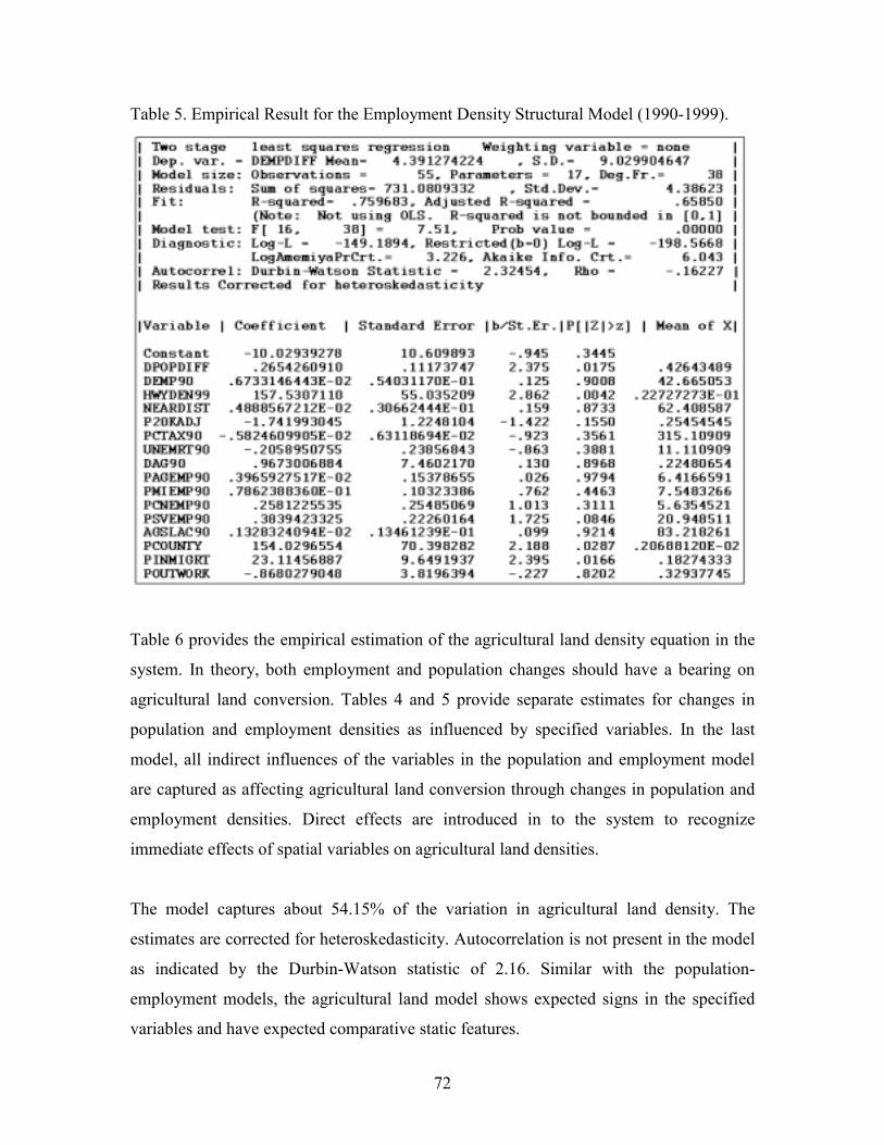
Table 5. Empirical Result for the Employment Density Structural Model (1990-1999).
Table 6 provides the empirical estimation of the agricultural land density equation in the
system. In theory, both employment and population changes should have a bearing on
agricultural land conversion. Tables 4 and 5 provide separate estimates for changes in
population and employment densities as influenced by specified variables. In the last
model, all indirect influences of the variables in the population and employment model
are captured as affecting agricultural land conversion through changes in population and
employment densities. Direct effects are introduced in to the system to recogniz
mediate effects of spatial variables on agricultural land densities.
variables and have expected comparative static features.
e
im
The model captures about 54.15% of the variation in agricultural land density. The
estimates are corrected for heteroskedasticity. Autocorrelation is not present in the model
as indicated by the Durbin-Watson statistic of 2.16. Similar with the population-
employment models, the agricultural land model shows expected signs in the specified
72

Table 6. Empirical Result for the Agricultural Land Density Change Model (1990-1999).
Generally, the empirical results provide important information about the land conversion
processes in West Virginia. The results are consistent with expectations and other
empirical results in the literature.
4.2. ANALYSIS OF RESULTS
The system of equations model results are generated from the two stages least squares
and ordinary least squares estimates. The employment and population density changes,
generated from the simultaneous interaction models are depicted in tables 4 and 5;
similarly output for agricultural land density is provided in table 6. This analysis focuse
ealing with land conversion indicators. The analysis for
e three models is given in the following separate sections.
s
on the interpretation of the econometric results, interaction of the three models and
comparative reference of the generated results with USDAs Natural Resource
Conservation Service GIS maps d
th
73

4.2.1. Analysis of the Population Density Model
In the model specification, change in population (population in 1999 minus population in
1990) is specified as one of the significant factors explaining the conversion of
agricultural lands. Population, though directly and indirectly interacting with changes in
agricultural lands, is by itself affected by a number of other explanatory factors. These
variables have an indirect bearing on agricultural lands through their direct effects on
opulation density changes.
y a number of reasons. One of them is
the spatial difference in fiscal burdens. The population density model indicates that per
apita tax areas while traveling to work in the metropolitan
reas. Such kinds of spatial features are expected to be observed in the Eastern
rovided in chapter three. Though there
re different ways of capturing access as a variable, interstate highway density
p
Population changes are explained in the literature b
capita tax in the base period (PCTAX90) is negatively related with changes in population
density, though the standard error of the variable is high. Following the result, it can be
expected that an increase in tax burdens in some areas may cause a decline in the
population growth in that area as tax burdens are minimized through relocation decisions.
Due to high tax burdens, for instance, a large number of people reside in adjacent non-
metropolitan and lower per c
a
Panhandle, Charleston, and other urbanized locations of influence. Hence, fiscal
attributes of locations can influence to a degree the location decision of households
responding to their cost and income constraints.
This result may be better explained if the sample included neighboring metropolitan
places and urbanized sites as tax burdens are typically higher and movement to regions of
low tax burdens (like West Virginia) may be evident. The West Virginia model, however,
still captures tax differential playing a role in influencing trends of population density
changes as evidenced by sign on PCTAX90 in Table 4.
Access, as a predictor of population density changes is well argued in the literature.
Comparative static results of the argument are p
a
74

(HWYDEN99) in each county and physical nearness to metropolitan areas (NEARDIST)
are selected as proxies to predict changes in population density.
According to population growth theories, it can be expected that nearness to metropolitan
areas and urbanized locations would affect population growth positively. However,
nexpected sign and high insignificance is found for the relationship between highways
n density.
and adjacent
cations.
tage of houses that are owner occupied (OWNOCC90) is significantly
ssociated with population density changes. The result indicates that rates of owner
u
and changes in population density in West Virginia. The result may indicate that since
interstate density in West Virginia is small and since the distribution of the interstate
network is limited to a few counties in the state, interstate highways may be a poor
predictor of changes in population density in the state. The results show an insignificant
influence of interstate highway in predicting changes in populatio
Nearness to metropolitan and urbanized areas demonstrates a demographic tendency that
as distance from these central locations increases, population density decays at some rate.
The negative coefficient for NEARDIST captures such a decaying nature of population
growth with distance. The result is intuitive in that as distance increases from central
places (to possibly rural locations), the transportation and other public facilities decline in
supply and economic cost of movement to distant areas (areas of job and frequently
visited recreational site) increases. This is an important result as similar population
patterns have a significant bearing on agricultural lands at the sub-urban
lo
The result for the relationship between adjacency to urbanized areas (P20KADJ) and
changes in population density indicates an insignificant negative relationship. This may
indicate that counties that are adjacent to urbanized areas do not significantly show much
difference in population change than the non-adjacent counties. This may imply that
population changes are not limited to adjacent counties but has spread to non-adjacent
rural counties.
The percen
a
75

occupancy positively affect density change in population. This makes sense in two ways.
First, that a higher rate of owner occupancy indicates that people decide to stay in that
location for an extended period of time, which positively affects the population density in
the location of settlement. However, beyond this obvious physical relationship one can
infer that higher rates of owner occupancy is normally observed, among many groups,
with in-migrating high income families and retired (senior) citizens. Hence, relating the
x burden analysis and the wealth of natural amenities in West Virginia, gradual
ulation density
hanges might indicate that the change in population is little affected by unemployment
ta
movement to West Virginia from surrounding high tax and less natural amenity supply
areas is possible. The spread of new retirement houses and recreational and residential
facilities in some parts of West Virginia is one justification for the result.
There is also a significant positive relationship between changes in population densities
and unemployment rates (UNEMPRT90). Intuitively, regions of high unemployment
attract fewer people through the employment and crime effects. The unexpected negative
sign in the population density model, however, may mean that across the 55 sample
counties in West Virginia, population density changes are higher in counties with higher
rates of unemployment. Generally, rural counties face higher rates of unemployment.
Furthermore, the positive relationship between unemployment and pop
c
considerations but rather by other factors. Again, the groups that are less averse to
unemployment are affluent and retired people. Thus, an inference may be made that the
change in population in West Virginia are affected by the natural growth rates as well as
by the influx of affluent and senior citizens as also evidenced by the high rates of owner
occupancy.
76

77
Fig. 9. New Acres of Developed Land in Non-Metropolitan Areas, 1992-1997.
Source: USDA, Natural Resources Conservation Service, Resource Assessment Division, Washington,
D.C., 2001.
Studies associate positively the relationship between population growth and pressure on
natural amenities. In a structural simultaneous equations model, for instance, Duffy-Deno
(1997) measured the pressure exerted on endangered species due to changes in population
and employment. A similar result is indicated between changes in population density and
natural amenities – percentage of agricultural land in water (PWATERAC) and
percentage of agricultural land in forest (PFORESTL) in this study. The model estimates
indicate a significant negative relationship between population change and forested
counties and a negative but insignificant relationship with density of surface water (lakes,
rivers).
Consistent with the model specification and sign expectation, the result may indicate that
high changes in population density is occurring in areas where there is decreasing

proportions of forest and water acres, which might indicate influences of the population
change on the stock of natural amenities.
Intuitively, inference can be made that if population change is influenced by nearness to
urbanized areas, then access (nearness) indirectly affects agricultural land conversion
through population pressures. (The result for agricultural land density and its relation to
ccess reinforces this analysis). Hence, the result supports that regions with more
rleston in the southwest, Morgantown in the
orth central and the Eastern Panhandle in the northeast parts of West Virginia. The spots
7 where the shaded federal
nd region in the southeastern part of West Virginia is free from significant development
a
exposure to urban influence attract higher rates of population and increase pressure on
natural endowments and agricultural lands. Figure 7 supports this result. The map
indicates new development spots that are highly spatially associated with nearness
(accessibility) to urbanized areas of Cha
n
are also regions of high population growth in West Virginia.
The relationship between population density changes and percentage of counties in
federal ownership (PFEDL) is also indicated in table 4. The result indicates a significant
inverse relationship between federal preservation programs and population density
changes. An increase in federal land will negatively affect population density changes,
i.e., federal land preservation programs can slow population growth in some regions. This
can happen in many ways. One possible way is that preservation programs, by limiting
the encroachment of residential land to federal land reserves, physically limit the spread
of population pressures. This is particularly evident in figure
la
pressures. Another way a federal land preservation program affects population growth is
through the effect on the value of land. By physically limiting the economic supply of
land to other uses, preservation programs can increase the market value of land hence
reducing the incentive to buy land. This can push development and housing demands of
land to neighboring counties where land reservations are not significant in affecting land
and property values. The interaction of these processes within the context of a large land
reservation program (like more than 65% for the southeastern region) hence negatively
influences the spread and growth of population.
78

The result also estimates a significant positive relationship between population density
changes and median housing value (MEDHVA90). The model estimate result for the
relationship between median housing value and change in population was not as
intuitively expected. The positive relationship may imply that higher population density
changes are occurring in areas of higher median housing value in West Virginia. This
may be due to the fact that regions of high population experience high demand for
properties. This can raise property values in the face of higher demands from increasing
population through time. This can yield a positive relationship between housing value
nd population concentration.
g, they are cheaper when compared to the adjacent
etropolitan D.C. area, making the Eastern Panhandle a substitute for the high property
agricultural activities.
a
However, it may also be argued that areas of growing housing and property value,
ceteris paribus, attract less population in-migration and hence slowdown the density
change in population. The data set does not account for the fact that though property
values are increasing in population centers in West Virginia, it could be true that still they
are relatively cheaper when compared to surrounding metropolitan and urbanized areas.
For instance, the housing value in the Eastern Panhandle is increasing at a significant
scale but still faces increasing demand. One reason for this could be the fact that though
property values are increasin
m
values in D.C. Since the study is concentrated in West Virginia, economic activities in
the surrounding states are not included in the dataset. The result can thus be attributed to
sampling limitations.
On the relationship between population density change and agricultural land density
(DAG90), the population density model estimates a negative relationship, which is
intuitive. This may imply that changes in population are associated with declining
agricultural lands. A growth in population not only requires increased public facilities, it
also requires housing, recreational, and other attendant land demanding necessities. This
comes in direct competition over the use of land, especially in areas of significant
79
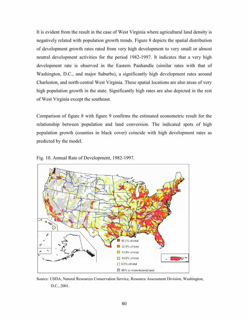
80
It is evident from the result in the case of West Virginia where agricultural land density is
negatively related with population growth trends. Figure 8 depicts the spatial distribution
of development growth rates rated from very high development to very small or almost
neutral development activities for the period 1982-1997. It indicates that a very high
development rate is observed in the Eastern Panhandle (similar rates with that of
Washington, D.C., and major Suburbs), a significantly high development rates around
Charleston, and north-central West Virginia. These spatial locations are also areas of very
high population growth in the state. Significantly high rates are also depicted in the rest
of West Virginia except the southeast.
Comparison of figure 8 with figure 9 confirms the estimated econometric result for the
relationship between population and land conversion. The indicated spots of high
population growth (counties in black cover) coincide with high development rates as
predicted by the model.
Fig. 10. Annual Rate of Development, 1982-1997.
Source: USDA, Natural Resources Conservation Service, Resource Assessment Division, Washington,
D.C., 2001.

81
This further justifies the conclusion that population change (rather than employment
driven changes) accounts for the major conversion situation in West Virginia. The growth
of population in locations of high unemployment rates and high median housing values
reinforces that population changes drive most of the population conversion than
employment generation, though they are also significant factors in explaining the
conversion of agricultural land to non-agricultural uses.
Fig. 11. Percentage Change in Population: 1990 – 1999.
Source: Adopted from U.S. Bureau of Census by Condon, Childs, and Bogdan, Bureau of Business and
Economic Research, West Virginia University, Sept. 2000.
The relationship between employment and population is addressed in some detail in the
specification. The results for the association of proportion of county jobs held by outside
county residents (PINMIGRT), proportion of residents employed outside the county
(POUTWORK), and changes with total employment density (EMPDIFF) are provided in

table 4. Generally, a positive relationship is found between changes in population density
with total employment changes and proportion of residents employed in a different
county while a negative relationship is found with proportion of county non-resident
employment.
The result may imply that counties with high proportion of employed residents who work
outside a county (bedroom communities), face high population density changes, and
counties with high proportion of resident jobs held by people outside the county face low
population changes. Joint consideration of the two results may indicate that changes in
population density are high in counties with favorable access to locations of urban
development. With considerations of urban negative externalities (congestion, crime and
safety, tax burden, etc), people may prefer to stay in suburban counties and work in cities
or urbanizing counties, as returns to efforts are higher. For example, high rates of
population increases are recorded in the Eastern Panhandle where significant number of
people work in Washington, D.C., metropolitan area and reside in the Eastern Panhandle
ounties. Similar behaviors are true around Charleston and major urbanizing locations in
ed
might contribute to the on going argument as to whether employment
llows jobs or jobs follow employment. From the result, it may be inferred that in the
c
West Virginia. Thus, the result might imply that population changes, and thus increas
competition for land, are high in the suburban counties.
The result also estimates a positive but insignificant relationship between population
density changes and employment change. This coefficient estimate directly tests the
relative influence of the simultaneous endogenous variable employment difference
(EMPDIFF) - on population density changes. Contributing to the debate on whether
population attracts employment or vice-versa, the results indicate that employment
creation has a positive, but statistically insignificant influence on population growth
trends in West Virginia as compared to the influence of population on employment
growth. This
fo
case of West Virginia the argument that employment changes drive population density
changes is rather weak.
82

To summarize the population density model, the following comparative static results for
West Virginia are confirmed by the results of the study:
∂(DPOPDIFF)/∂(NEARDIST) < 0, ∂(DPOPDIFF)/∂(P20KAD) < 0, ∂(DPOPDIFF)/∂(OWNOCC90) > 0,
∂(DPOPDIFF)/∂(UNEMPRT90) > 0, ∂(DPOPDIFF)/∂(PWATERAC) < 0, ∂(DPOPDIFF)/∂(PFORESTL)
< 0, ∂(DPOPDIFF)/∂(PFEDL) < 0, ∂(DPOPDIFF)/∂(MEDHVA90) > 0, ∂(DPOPDIFF)/∂(DAG90) < 0,
4.2.2. Analysis of the Employment Density Model
The employment model captures significant information
∂(DPOPDIFF)/∂(PINMIGRT)< 0, ∂(DPOPDIFF)/∂(POUTWORK) > 0, ∂(DPOPDIFF)/∂(DEMPDIFF) > 0.
concerning employment density
hanges and their relationship to key variables of research interest. Table 5 summarizes
d access implies that locations endowed with better access (for
xample, interstate highways) attract more employment opportunities as access reduces
abeled at different growth rates.
terestingly, such spatial clusters of employment growth are associated with access.
infrastructure amenities. This result can be compared with figures 10 and 11 that shows
c
the output for the econometric estimation.
On the influence of access to employment density changes, the result indicates a
significant positive relationship between employment changes and improved access.
Specifically, a significant positive relationship is observed between employment growth
and highway density (HWYDEN99) while a weak positive relationship is estimated for
the relationship with the distance from nearest metropolitan county (NEARDIST)
measure.
Consistent with logical expectations, the significant positive relationship between
employment and improve
e
the costs of transportation and exposes new markets separated by transportation barriers.
Figure10 indicates regions of high population growth l
In
Employment growth centers are centered significantly across regions of high access of
that employment densities and location of interstate highways are spatially correlated.
83
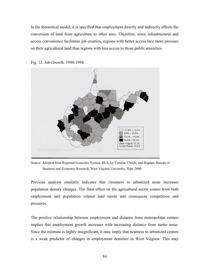
84
In the theoretical model, it is specified that employment directly and indirectly affects the
conversion of land from agriculture to other uses. Therefore, since infrastructural and
access convenience facilitates job creation, regions with better access face more pressure
on their agricultural land than regions with less access to those public amenities.
Fig. 12. Job Growth: 1990-1998.
Source: Adopted from Regional Economic System, BEA, by Condon, Childs, and Bogdan, Bureau of
Business and Economic Research, West Virginia University, Sept. 2000
Previous analysis similarly indicates that closeness to urbanized areas increases
population density changes. The final effect on the agricultural sector comes from both
employment and population related land needs and consequent competition and
pressures.
The positive relationship between employment and distance from metropolitan centers
implies that employment growth increases with increasing distance from metro areas.
Since the estimate is highly insignificant, it may imply that nearness to urbanized centers
is a weak predictor of changes in employment densities in West Virginia. This may

further indicate that changes in employment densities are occurring in locations that are
not close to urbanized locations. In addition, the employment growth occurring in West
Virginia may be heterogeneously distributed beyond the speculated urban expansion
effects.
Fig. 13. Interstate Road Map: West Virginia.
Source: Adapted from Natural Resource Analysis Center GIS resources, West Virginia University.
The model result for the relationship between adjacency to urbanized areas and changes
in employment densities indicates an insignificant and negative relationship. This may
imply that counties that are adjacent to urbanized areas showed no significant difference
in employment than those that are not adjacent. This may further imply that employment
growth is not significantly limited to adjacent counties, but rather is dispersed in non-
adjacent counties as well.
85

The employment density model estimates a negative relationship between per capita
taxes and employment density changes. Theoretically, firms choose locations that
minimize the total costs of the operation. If costs vary across space, then mobility of
firms across space to capture cost advantages is expected. Similarly, the result indicates
that employment growth is negatively associated with high tax locations as firms may
relocate to take advantage of tax structures that vary across space. This result is
consistent with theoretical expectation that firms will be less attracted to regions of high
tax burdens.
A negative relationship between employment density growth and unemployment rates
(UNEMPRT90) is observed in the result indicated in table 5. Though it may be argued
that regions of high unemployment have lower labor costs that could attract employment
growth, it is not justified in the case of West Virginia. Given the nature of employment
growth, a high proportion of growth is observed in the service sector. Such services (like
fast food, malls, recreational facilities) are spread across areas of high population
owing
ounties). Hence, it could be possible that the lower income of high unemployment areas
ifferent sectors. The relevant sectors of analytical interest are
e percentage of employment in the agricultural (PAGEMP90), mining (PMIEMP90),
significantly and directly related with counties dominated by the service sector.
growth (demand factor) and areas of better purchasing power capacity (fast gr
c
and high poverty counties could have adverse negative implications on employment
growth opportunity.
The change in employment, in the model specification, is decomposed into different
sectors of interest to capture the sources of employment density changes through
employment changes in d
th
construction (PCNEMP90), and service (PSVEMP90) sectors. The results from the
model indicate that construction, mining, and agricultural sector employment have a
positive but highly insignificant relationship with changes in total employment. The
agricultural sector in particular poorly explains total changes in employment density in
West Virginia. This may imply that these sectors account for insignificant variation in
employment density changes in the state. However, a change in employment density is
86

Figure 10 indicates higher rates of employment growth, which are basically concentrated
in areas of high population density. The growing percentage of employment in the service
nd construction industry might infer the spread of service based new industries and
del estimates a positive relationship between agricultural sales
LAC90) and employment density changes. Intuitively, it could be expected on the
positive
ales per acre as production switches to high valued crops. In a way,
a
emerging construction activities in the state. Growth in the service sector may generate
new employment opportunities. This can negatively influence employment in the
agricultural sector.
From this result, it can indirectly be inferred that pressure on agricultural employment
and hence, on the viability of the agricultural sector across regions is influenced by the
growing new economy. The implication on agricultural land conversion thus becomes
evident.
Interestingly, the mo
(AGS
contrary that changes in non-agricultural employment may exert pressure on the
agricultural sector affecting the income and feasibility of the agricultural sector.
However, the result opens room for many possible educated guesses. Ambiguously, the
increase in employment and population in the suburban and other high employment
growth areas can be thought of as a source of growing agricultural output market for local
farmers. This may mean that not only do negative externalities caused by development
exist, but also there are positive externalities associated with market creation for farm
products. Nonetheless, a critical argument can also be raised that since employment
competes for land and labor with the agricultural sector, negative effects on the
agricultural sector may be encountered. This ambiguity leads to the direction of marginal
effects with increasing employment and purchasing power growth, does the
effect of market creation exceed the negative effect of resource conversion to other
sectors? This by itself could be an area of separate research. For the purpose of current
analysis though, it would be enough to recognize the possible external benefits of
employment growth to agricultural market extension as evidenced by the result of the
model. It is expected that specialty markets for agricultural products would result in
higher agricultural s
87

the result is recognizing the fact that employment growth need not necessarily have only
deral land preservation programs, the result indicates a positive and significant
lationship between proportion of land owned by a county and changes in employment
nt issues, it can further be linked that counties with better employment growth
nd access can experience changes in in-migrating labor that may significantly affect
negative effects on the agricultural sector, but could possibly support some market
creation.
Unlike fe
re
density. With the federal land preservation program, it was indicated that it slows
changes in population density and might push development pressures to counties with
significantly less federal land preservation. However, the result for the relationship when
a county owns proportionate land is significantly positive which may imply that counties
with significant land ownership saw significant changes in employment. This may be due
to the fact that such counties might provide incentives on their county land to encourage
employment opportunity growth and development to overcome poverty and development
bottlenecks in the state. Through the model set up, this will have an indirect effect on the
conversion of agricultural lands to such development uses.
Incorporating labor mobility aspects into the employment density model, a significant
positive relationship is estimated between total employment changes and the proportion
of resident county jobs held by people outside a county. This indicates that a high change
in employment density is associated with counties that draw workers from neighboring
areas. Generally, labor migrates to areas of better probability of employment and areas of
high return per supply of labor effort. However, in this case, people are commuting from
adjacent counties for employment, potentially due to the shortage of a labor force in the
county with jobs.
Figure 10 depicts counties in West Virginia experiencing different rates of job growth.
Associating the result with previous discovery on the association of access and
employme
a
changes in total employment densities. Since the employment density model predicted an
insignificant relationship between changes in agricultural employment and changes in
88

total employment densities and a significant positive association with service sector
growth, this labor in-migration result might imply some degree of pressure on
agricultural lands excreted by non-agricultural sector pressures.
On the other hand, counties with bedroom communities (proportion of resident labor
employed outside the county) experienced negative changes in employment density.
Though intuitive, the result is highly insignificant. Intuitively, counties with high
proportion of resident labor force working outside the county face lower changes in
employment density. Better compensation and incentives can attract county labor to
pply their effort outside the county. With increasing significance of bedroom
rced in the employment model. A change in population significantly
fluences employment growth. One inference that can be generated from this result is
of West Virginia for the
onsidered period of 1990 1999/2000.
su
communities, a slower growth in employment in a county could be experienced.
A positive relationship is also found in the result on the relationship between changes in
employment density and population changes. The significant positive relationship
between population changes (POPDIFF) and employment density change provides
further information to the previous result on whether people follow jobs or jobs follow
people argument presented in the previous section. The conclusion that jobs follow
people is also reinfo
in
that combining the results from the two models, population pressures account for higher
land conversion influences than employment growth in West Virginia.
Figure 12 reinforces the conclusion from the model by indicating that for the northeastern
region in general, residential (household) demand accounts for a significantly higher rate
of agricultural land conversion (72% of the converted crop land, while for business
purposes it stands at 14%) to non-agricultural uses for the 1982 1992 period. Though
employment also significantly interacts in the conversion process, its effect is relatively
less that population pressures. This result also holds for the case
c
89
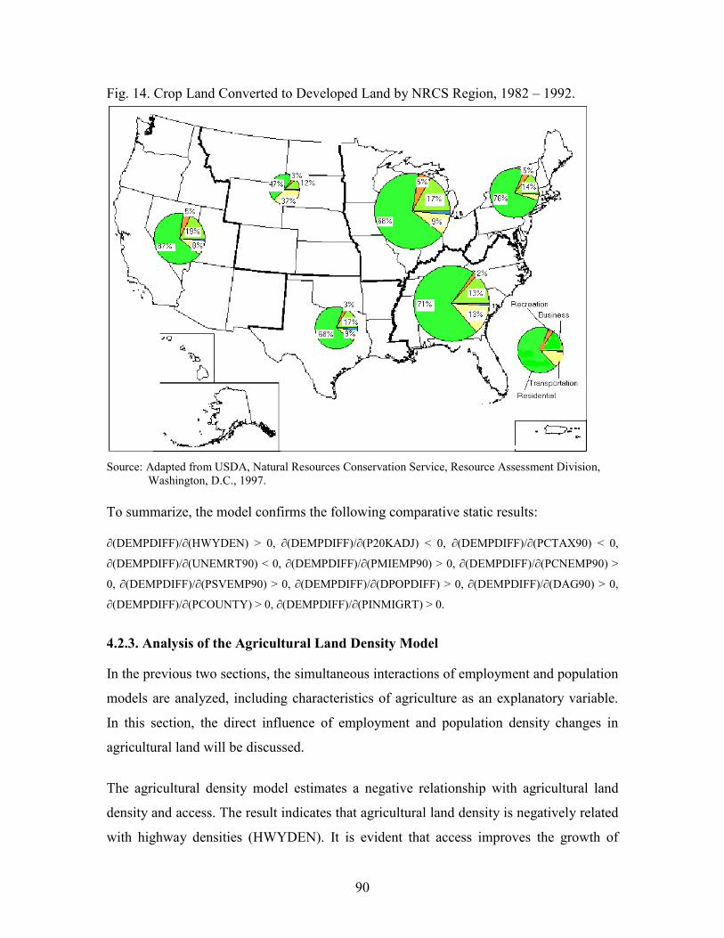
90
Fig. 14. Crop Land Converted to Developed Land by NRCS Region, 1982 – 1992.
Source: Adapted from USDA, Natural Resources Conservation Service, Resource Assessment Division, Washington, D.C., 1997. To summarize, the model confirms the following comparative static results: ∂(DEMPDIFF)/∂(HWYDEN) > 0, ∂(DEMPDIFF)/∂(P20KADJ) < 0, ∂(DEMPDIFF)/∂(PCTAX90) < 0,
∂(DEMPDIFF)/∂(UNEMRT90) < 0, ∂(DEMPDIFF)/∂(PMIEMP90) > 0, ∂(DEMPDIFF)/∂(PCNEMP90) >
0, ∂(DEMPDIFF)/∂(PSVEMP90) > 0, ∂(DEMPDIFF)/∂(DPOPDIFF) > 0, ∂(DEMPDIFF)/∂(DAG90) > 0,
∂(DEMPDIFF)/∂(PCOUNTY) > 0, ∂(DEMPDIFF)/∂(PINMIGRT) > 0.
4.2.3. Analysis of the Agricultural Land Density Model
In the previous two sections, the simultaneous interactions of employment and population
models are analyzed, including characteristics of agriculture as an explanatory variable.
In this section, the direct influence of employment and population density changes in
agricultural land will be discussed.
The agricultural density model estimates a negative relationship with agricultural land
density and access. The result indicates that agricultural land density is negatively related
with highway densities (HWYDEN). It is evident that access improves the growth of

91
employment in a region, as confirmed by the employment model in the last sections. At
the same time, it also tends to diminish agricultural land densities due to increased
pressure. The result is confirmed by the negative comparative static result for the
agricultural land - access relationship. Expansion of highways has facilitated the increase
in population and employment concentrations directly impacting land holdings for
different agricultural activities.
Fig. 15. Acres of Non-Federal Developed Land, 1997.
Source: Adapted from USDA, Natural Resources Conservation Service, Resource Assessment Division, Washington, D.C., 2000.
As indicated in figure 13, development pressures are highly associated with road
infrastructure developments in West Virginia. This can be inferred by comparing the
distribution of development spots with interstate road developments (figure 11). This
result is consistent with the conclusions that agricultural land conversion intensifies near
transportation facility developments and decays as distance from accessed areas
increases.

The positive result describing the relationship between changes in agricultural land and
nearness (NEARDIST) to urbanized centers was not theoretically expected. The direct
effect of distance on agricultural land conversion was expected to decay as distance
increased from the urbanized centers. However, the estimated relationship is highly
insignificant and could be a poor proxy to capture locational variation through physical
istance.
A more appropriate measure of the influence of location on agricultural land conversion
may be the adjacency dummy proxy (P20KADJ) that measures the influence on rural
communities of being adjacent to urbanized areas as compared to not being adjacent to
urbanized locations. The result, at a 2 percent significance level, indicates that those
counties that are adjacent to urbanized areas experienced 37.9% more changes
(variations) in their agricultural land density as compared with those counties that are not
adjacent to urbanized locations. This result can be related with the finding in the
population density model that agricultural lands density is negatively related with
changes in population density. Generally, higher population pressure is expected in
urbanized and suburbanized locations that have more pressure on land for growing non-
agricultural purposes. From this perspective, it can be inferred that counties that are
adjacent to urbanized locations experiencing 37.9% more variation in their agricultural
land density have more pressure on land use and allocation that may negatively affect
agricultural land densities.
tion growth concentration in West Virginia. Significant
lusters of population growth can be observed adjacent to urbanized and sub-urbanized
gricultural land density occur in areas where there are high changes in
population density. This result is logically consistent with the theoretical expectation that
d
Figure 14 indicates popula
c
areas.
On the relationship between changes in population density (DPOPDIFF) and agricultural
land density (DAGDIFF), the relationship estimate shows (in table 6) a positive
relationship between the two endogenous variables. This result indicates that high
changes in a
92
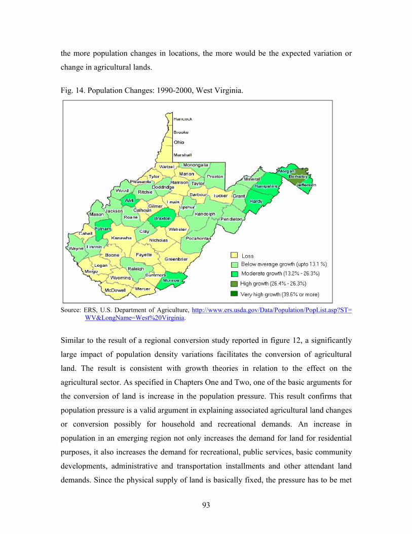
93
the more population changes in locations, the more would be the expected variation or
change in agricultural lands.
Fig. 14. Population Changes: 1990-2000, West Virginia.
Source: ERS, U.S. Department of Agriculture, http://www.ers.usda.gov/Data/Population/PopList.asp?ST= WV&LongName=West%20Virginia.
Similar to the result of a regional conversion study reported in figure 12, a significantly
large impact of population density variations facilitates the conversion of agricultural
land. The result is consistent with growth theories in relation to the effect on the
agricultural sector. As specified in Chapters One and Two, one of the basic arguments for
the conversion of land is increase in the population pressure. This result confirms that
population pressure is a valid argument in explaining associated agricultural land changes
or conversion possibly for household and recreational demands. An increase in
population in an emerging region not only increases the demand for land for residential
purposes, it also increases the demand for recreational, public services, basic community
developments, administrative and transportation installments and other attendant land
demands. Since the physical supply of land is basically fixed, the pressure has to be met

by changing the economic supply of land through reallocation from other sectors. In
suburban fringes and rural areas, where the dominant economic activity could be
griculture, this sector faces growing challenges of economic, legal, and administrative
lt. Ultimately, this results in
conversion of agricultural lands to meet growing population needs. The result for West
Virginia indicates similar tendencies.
However, a specific argument can be raised about what particular agricultural land use is
typically affected by the conversion pressures. Modeling agricultural lands classified into
two major uses cropland (PCROP90) and pastureland (PPAST90) the result in the
agricultural density model indicates that croplands are positively related with changes in
agricultural land density while pastureland is negatively related with the total agricultural
land density changes. The proportion of cropland is modeled as a proxy for prime
farmland establishing a rational expectation that farmers will allocate their land according
to the priority that best lands are put into crops and relatively marginal lands are set aside
for pasture land and other relevant agricultural activities. Thus, the relationship with
cropland indirectly captures changes in prime farmland.
more cropland. In addition, areas with a greater proportion of farmland in pasture saw
smaller changes in farmland. This may indicate that in those counties or areas where
farmland conversion is intensified, croplands and consequently prime farmlands are
primarily affected. The negative effect on croplands could be due to the features of such
lands. In many instances, croplands are flatter and more convenient to development than
are pasturelands, woodlands, or other agricultural land uses making cropland even more
sensitive to development pressures. The conversion of other agricultural land uses is
relatively more costly than the conversion of croplands for development purposes.
a
pressures making sustained farming practices difficu
From the result, it may be inferred that the loss of farmland coincides with areas having
94

This can be better understood with the visualization of the structure of the agricultural
sector in West Virginia. Baniecki and Dabaan (1998) report:
Poultry, meat animals, and dairy dominate the farm economy in the Mountain State. Commercial broiler production has shown a dramatic increase over the last ten years with the value of production increasing from $29.4 million in 1985, to $52.2 million in 1990 to $139.0 million in 1997. The relatively small field crop acreages are mainly devoted to livestock feeds. Of the 6371997, 88 percent are hay, 10 percent cor
,000 acres harvested from principal field crops in n, 1 percent wheat, and 1 percent oats. Based on
1997 cash receipts of over $393 million, the top ten commodities are: broilers, 35 percent; cattle and calves, 18 percent; dairy products, 9 percent; eggs, 6 percent;
The agricultural land density model provides interesting information about the nature of
the agricultural sector and related tendency to conversion. The relationship between
agricultural sales (AGSLAC90), agricultural employment levels (PAGEMP90), and
agricultural land density change is estimated in table 6. Interestingly, the result indicates
that agricultural sales and agricultural employment are significantly negatively related
with changes in agricultural land density.
he result indicates that the less profitable and competitive agriculture is, the more
he protection of agricultural land can be addressed from two directions: government
servation programs and increasing the profitability of the agricultural sector. Without
greenhouse and nursery, 4 percent; hay, 3 percent; apples, 3 percent; corn, 2 percent; and peaches, 1 percent. Other livestock related commodities important to West Virginia's economy are sheep and lambs and hogs. Apple and peach orchards cover about 9,000 acres in the State. Burley tobacco harvested, although only 1,800 acres, ranks fifteenth in production.10
T
conversion of agricultural lands to other uses would be expected. This result is clearly
intuitive and logically consistent with the theoretical setup that economic agents that can
provide a higher bid rent for a given land at a particular distance and location will
dominate that location. Conversely, a rise in agricultural sales and employment
opportunities should lead to lower agricultural land density declines. From this interesting
comparative static result, it can be inferred that the conversion of agricultural lands to
other uses observed in this study can partly be justified by the relatively lower sales
performances and declining shares of employment creation in the agricultural sector.
T
re
See report at http://www.wvu.edu/~agexten/ipm/pestprog/NAPIAP/agricult.htm#Agriculture10 .
95
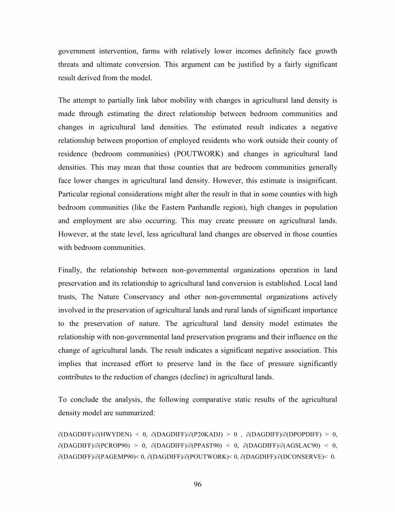
government intervention, farms with relatively lower incomes definitely face growth
threats and ultimate conversion. This argument can be justified by a fairly significant
result derived from the model.
The att sity is
made t s and
change ative
relation ty of
residen nd
densitie erally
face lower changes in agricultural land density. However, this estimate is insignificant.
Finally, the relationship between non-governmental organizations operation in land
To conclude the analysis, the following comparative static results of the agricultural
∂(DAGDIFF)/∂(HWYDEN) < 0, ∂(DAGDIFF)/∂(P20KADJ) > 0 , ∂(DAGDIFF)/∂(DPOPDIFF) > 0,
AGDIFF)/∂(PCROP90) > 0, ∂(DAGDIFF)/∂(PPAST90) < 0, ∂(DAGDIFF)/∂(AGSLAC90) < 0,
∂(DAGDIFF)/∂(PAGEMP90)< 0, ∂(DAGDIFF)/∂(POUTWORK)< 0, ∂(DAGDIFF)/∂(DCONSERVE)< 0.
empt to partially link labor mobility with changes in agricultural land den
hrough estimating the direct relationship between bedroom communitie
s in agricultural land densities. The estimated result indicates a neg
ship between proportion of employed residents who work outside their coun
ce (bedroom communities) (POUTWORK) and changes in agricultural la
s. This may mean that those counties that are bedroom communities gen
Particular regional considerations might alter the result in that in some counties with high
bedroom communities (like the Eastern Panhandle region), high changes in population
and employment are also occurring. This may create pressure on agricultural lands.
However, at the state level, less agricultural land changes are observed in those counties
with bedroom communities.
preservation and its relationship to agricultural land conversion is established. Local land
trusts, The Nature Conservancy and other non-governmental organizations actively
involved in the preservation of agricultural lands and rural lands of significant importance
to the preservation of nature. The agricultural land density model estimates the
relationship with non-governmental land preservation programs and their influence on the
change of agricultural lands. The result indicates a significant negative association. This
implies that increased effort to preserve land in the face of pressure significantly
contributes to the reduction of changes (decline) in agricultural lands.
density model are summarized:
∂(D
96

CHAPTER V
SUMMARY AND CONCLUSION
ses on the case of West Virginia where development
pressures along urbanized and semi-urban locations are believed to compete most
Different studies substantiate that with ever growing cities and expanding urban
boundaries, a significant conversion of agricultural land to other uses has occurred. The
implications of this growing trend in the conversion of agricultural land to other uses
5.1. SUMMARY
The relationship between mankind and the environment and resources is an intricate one.
With ever growing population and social needs, the resulting strain on natural resources
is increasing. One of the natural resources of particular importance is land. As the
economy grows, there is increased pressure over the use of land.
The objective of this study is the investigation of factors associated with spatially varying
land use changes; in particular, agricultural land changes. The loss of agricultural land is
evident in the United States as the growth of other non-agricultural sectors demand more
land, creating direct and indirect pressure on agricultural land conversion nationwide.
This study particularly focu
strongly with agricultural uses of land.
Land value and land use changes are areas of study in economic history since Adam
Smith. Treating land as any other economic good, it is demanded by consumers to
maximize their utility attached to locations and by producers to maximize profits that
vary across locations. The interaction of these forces and the resulting location bid rent
determines the land use feature of different locations. That is, land will be put to its
highest and best (most valuable) use.
have been a focus of much concern and research. The concern over the loss of
agricultural land includes losses of rural character and environmental and other natural
amenities associated with farming practices.
97

Generally, spatial land use changes with regional economic
patterns that can fairly be captured by decision behaviors of households and firms. The
spatial preference of people emanates from their desire to maximize utility that varies
depending on what location is preferred for residential or recreational purposes. With
growing congestion, urban pollution, crime, and a number of urban attendant
reference of people has shifted to sub-urban and accessible rural
in the population and structural composition of rural lands directly interfering with rural
Similarly, business enterprises (firms) adjust their locations to minimize costs across
different locations. With growing population along the suburban and urban fringes,
and in those locations. The implication of these
trends on the agricultural sector is the main focus for this study.
sector attributes, a system of equations model is specified. The model follows from the
work of Carlino and Mills with relevant adjustments to address the research objective.
in the system focuses on agricultural land density
changes as a function of employment and population changes as well as a vector of other
conversion.
through time are associated
externalities, the p
locations where the urban-associated externalities are minimal and offer additional
natural amenities and other rural attendant external benefits. This has attracted a change
economic practices typically agricultural activities.
different service based industries and other business activities have intensified in order to
capture the newly emerging markets and labor cost advantages.
The interaction of these business and household decisions to maximize gains across
locations results in a re-allocation of l
To systematically capture the interaction of different growth factors and agricultural
The model captures the influence of population and employment density changes on
agricultural land. A separate equation
factors. The model captures regional economic changes, in terms of population and
employment distribution across space, and translates the impacts to the rate of land
98
Results indicate that population density changes are negatively associated with natural
amenities, federal lands, density of agricultural lands, per capita taxes, and distance from
urbanized and suburbanized places, while highways, employment growth, and owner
occupied housing positively influence the change in population density.
The employment density model results indicate that access, population growth,
construction and service sector employment dominance, and agricultural sales are
positively related with employment density expansions. Unemployment rate, agricultural
employment and distance are found to be negatively associated with employment density
changes.
The agricultural land density model reinforces the argument that agricultural land
conversion is motivated by population pressure, highway expansion, nearness of
metropolitan and urbanized centers, and weak agricultural sectors. The model
consequently captures the sources of pressure on agricultural land conversion and isolates
articular activities of agricultural land use affected by the conversion process. The result
.2. CONCLUSION
ding to the derivation of necessary implications.
p
is believed to provide relevant information for the ongoing land use issues in West
Virginia.
5
Modeling the interaction of intricate economic phenomena occurring in spatial
dimensions is a very challenging task. In light of this challenge theories assist in focusing
on specific relationships among variables of economic interest without making any
attempt to make them exhaustive or overly detailed.
This study relied on established structural growth modeling techniques to derive relevant
conclusions about agricultural land conversion in West Virginia. Following the structure
of the model and the behavior of the states economy, relevant results have been
identified lea
99

The study focused on factors that are directly and/or indirectly associated with changes in
agricultural land density from 1990 to 1999. Following is a summary of the research
results.
A. The population Density Model
Population density is expected to vary inversely with distance from identified
metropolitan, urbanized, and semi-urbanized areas, as transportation cost will
increase offsetting savings from lower property values and high natural amenities.
Population density is estimated to vary inversely with per capita tax burden,
which is unevenly distributed across different locations.
The density of highway systems is insignificant and negatively related to
population density changes across the state.
Population density change is negatively related with agricultural land density.
Federal land ownership reduces the expansion of population densities by the
physical protection on the conversion of land for development uses.
The rate of owner occupied housing in regions is positively related population
density changes.
Population density is negatively related with the stock of natural amenities. A
negative relationship is isolated between population densities and the percentage
by forest and water resources. of land covered
Population density changes are positively linked with unemployment rates.
A change in employment density will positively influence population density
changes.
Change in population density is negatively related with proportion of resident jobs
held by people outside the county and positively related with proportion of
employed residents who work outside their county of residence
100

B. The Employment Density Model
Change in employment density is positively affected by population changes.
Population growth is found to be significantly attracting employment changes in
West Virginia.
Changes in employment density are inversely related with per capita taxes.
Employment density changes are positively related with access endowments.
Highway density is found to affect employment growth.
The change in employment density is insignificantly related to employment in the
mining, agricultural, and construction sectors, but significantly and positively
related with service sector employment.
An inverse relationship is captured between unemployment rate and employment
density changes.
Employment densities are found to be positively related with agricultural sales.
upport some
This result possibly recognizes that employment growth need not necessarily have
only negative effects on agricultural sector, but could possibly s
market creation.
Counties with hig h county land ownership have a significant positive relationship
with changes in employment density.
Change in employment density is positively and significantly related with
proportion of resident jobs held by people o
utside the county and negatively
ty of
C
related with proportion of employed residents who work outside coun
residence.
. The Agricultural Land Density Model
High agricultural land density changes are associated with high population density
changes. Thus population growth is the driving force behind farmland co
nversion
in West Virginia.
Transportation access is negatively associated with agricultural land densities. By
directly claiming land and by intensifying other economic activities concentrated
around the accessed locations, the expansion of highways facilitates the
conversion of agricultural lands.
101

Decomposition of agricultural land uses into different specific use types indicates
armland, as proxied by cropland.
that the density of agricultural land is positively related with croplands and
negatively related with pasturelands. This indicates that West Virginia may be
losing its prime f
The decline in both agricultural sales and agricultural employment will facilitate
s for land.
the conversion of agricultural lands. This means that less competitive and
profitable agriculture is most at risk to alternative demand
A negative relationship is found between bedroom communities and changes in
agricultural land densities.
Non-governmental land conservation ini tiatives reduce the change in (conversion
It is b l
on the
stone fo
5.3. PO ENDATIONS
The stu ip between population, employment, and
agricu
agricul
the thre
that gro ime in population and employment has to be compromised with the
gricultural sector on the use and allocation of land.
Partic
agricul
affect a s they face more pressure from non-agricultural sectors through
time.
Though markets allocate resources efficiently under conditions of perfect competition,
assumptions of zero externalities of the perfect competition model is violated in the case
of agricultural lands. In many cases, agricultural lands not only provide agricultural
of) agricultural lands.
e ieved that the results and conclusions derived from this study will shed some light
ongoing issue of land conversion in West Virginia and could provide a stepping-
r further studies, inquiries, and improvements.
LICY RECOMM
dy addresses the intricate relationsh
ltural lands. Analysis of the three separate models of population, employment and
tural land densities provided extensive information on the nature and interaction of
e forces of interest. From the results, summarized in section 5.2, it can be noted
wth over t
a
ularly, the agricultural density model estimated that the poor performance of the
tural sector in terms of farm sales and employment generation will negatively
gricultural lands a
102

produ
values
values,
values.
On the
compar s may in this
case em
employ ties to the state. Recent highway extension programs
and o
From a encouragement of development per se may not be objected
ed and tallied with the marginal
benefits of new development undertakings.
In this study, the effects of tax structures, housing values and ownership, employment
ards agricultural land management
and protection need to properly consider the role and participation of federal and non-
land use policy should be introduced in the state of West Virginia to address both
development targets and agricultural land preservation. To overcome regional variability
cts to society or land to non-agricultural uses, it is also a source of non-market
in terms of preservation of the farming tradition, landscape preservation, scenic
and other positive externalities to society that may not be represented in land
other hand, West Virginia has a lower economic standard and economic growth as
ed to the rest of the United States. Economic development objective
phasize the encouragement of new developments in the hope of generating more
ment and growth opportuni
ther development packages are indications of this maintained desire.
policy perspective, the
from the perspective of the states economic development agenda. However, the proper
management of growth and its implication to the established local and rural economic
activities need to be properly evaluated and consider
and population expansion on agricultural lands are established and discussed. Policies
focusing or affecting such important areas need to take proper judgment as to the possible
implications on the agricultural communities.
Conservation (public and private) is found to significantly affect the conversion of
agricultural land to other uses. Policies oriented tow
governmental agencies in the effective management of the agricultural landscape.
Finally, to efficiently manage regionally varying developments and agricultural lands, a
proper
of land use structure, county level land use management practices may be introduced to
flexibly address the growing patterns of land use problems in the state.
103

5.4. LIMITATIONS OF THE STUDY AND AREAS OF FURTHER RESEARCH
The study of land use changes and identification and modeling of forces explaining the
land allocation process is a challenging task. Consideration of the issue at the broader
state level complicates the study and proper investigation of land use changes through
rium model is
introduced to study the land use issue in West Virginia and relevant conclusions are made
time.
This study provides relevant information and analysis about the land use trend in West
Virginia. A proper relationship between land use and relevant sources of influence
affecting the land use system is introduced and analyzed. A growth equilib
based on the findings.
However, the study faces its own limitations that can be summarized as follows:
Scope: the study focuses on West Virginia and systematically isolates the effects
of regional changes of important variables as constant. However, with the new
economy, the interaction of regions is highly correlated. Today, there is growing
interdependence among states and regions in terms of policy, trade, and many
other areas of interaction. Hence, modeling land conversion with a state level
frame has its own shortcoming.
Policy: the influence of policy measure directly and indirectly related with
agricultural land have a bearing on land use. West Virginia does not have an
explicit policy to address land use and growth management. However, such
policies are adopted and implemented in the Northeastern Region and their
implication in terms of growth dispersion and other attendant implications are not
captured. With a broader regional scope, a proper integration of policy variables
will help explain the land conversion processes and their marginal effects on
limiting or directing growth, and conserving agricultural land.
Spatial measures: it is evident that the location of an activity will have a
significant effect on land. Establishing the proper proxy and/or variable to
104
represent the effect of spatial location on land use is vital. Physical distances,
adjacency to urbanized areas, and interstate highway proxies are taken to
represent spatial locations. However, such measures can be improved by
integrating applied GIS spatial measures to properly establish the influence of
location on land use changes.
Modeling: this study models the change in land uses using a static system of
Thus, further research in this area can effectively be pursued by incorporating a
spatial
m a
equations growth model, applied to a single decade. Initial conditions are
compared with values at the end of the decade. However, approaching the
problem from a dynamic model may provide a better understanding of how
different forces interact in land use changes.
dynamic analysis of land use changes, that includes policy and effective
e sures, in a regional growth modeling framework.
105
BIBLIOGRAPHY
nso, William. Location and Land: Toward a General Theory of Land Rent.
vard University Press. 1964.
erson, W. D., G. C. Gustafso
1. Alo
Har
2. And n and R. F. Boxley. Perspectives on Agricultural
Land Policy. Journal of Soil and Water Conservation, 30(1): 1975.
3. Barkley, Paul W. and Gene Wunderlich. Rural Land Transfers in the United States.
USDA/ERS, Agricultural Information Bulletin No. 574, October 1989.
4. Barlowe, Baleigh. Land Resource Economics: The Political Economy of Rural and
Urban Land Resources Use. Prentice-Hall, Inc., Engelwood Cliffs, NJ. 1958,
5. Berry, David. Effects of Urbanization on Agricultural Activities. Growth and Change,
6.
ries No. 88. University of
Massachusetts, Amherst, 1976.
7. Bevan, Wilson Lloyd. Sir William Pett A Study in English Economic Literature.
Publications of the American Economic Association, Vol. IX, No. 4. 1894.
8. Brewer, M. F. and R. F. Boxley. Agricultural Land: Adequacy of Acres, Concepts and
Information. American Journal of Agricultural Economics, 63(5): 1981.
9. Brooks, Douglas H. Land Use in Economic Theory: Principles and Prospects.
USDAERS Staff Report Number Age870806. Washington, D.C., September 1987.
10. Brueckner, Jan K. and David A. Fansler. The Economics of Urban Sprawl: Theory
and Evidence on the Spatial Sizes of Cities. The Review of Economics and Statistics.
65(3): August 1983.
11. Brueckner, Jan K.. The Structure of Urban Equilibria: A Unified Treatment of the
Muth-Mills Model, 1982, in Mills, Edwin S., ed., Handbook of Regional and Urban
Economics, Vol 2, Amsterdam: North Holland-Elsevier Publishers. 1987.
12. Cantillon, Richard. Essai sur la nature du commerce en general, 1755.(English
Translation).[Online] available from http://socserv2.socsci.mcmaster.ca/~econ/ ugcm/
9(3): 1978.
Berry, David. Idling of Farmland in the Philadelphia Region, 1930-1970. Regional
Science Research Institute. Discussion Paper Se
y:
3ll3/cantillon/essay1.txt; accessed 14 September 2002; Internet.
106

13. Carlino, Gerald A. and Edwin nts of County Growth. Journal
Of Regional Science. 27(1): 1987.
of Rural Studies 2(1): 1986.
52(1): 1986.
wth. English.
17. ve the
18. , Kevin T. Economic Effect of Endangered Species Preservation in the
19.
20. of Agricultural Land Preservation. American Journal
21. Quarterly
22. Service in
23.
Report of the Sustainable Use of Land Project. Island Press,
24.
rty Values.
S. Mills. The Determina
14. Daniels, Thomas L. Hobby Farming in America: Rural Development or Threat to
Commercial Agriculture? Journal
15. Daniels, Thomas L., and Arthur C. Nelson. Is Oregon's Farmland Preservation
Program Working? Journal of the American Planning Association,
16. Deller, Steven C., Tsung-Hsiu (Sue) Tsai, David W. Marcouiller, and Donald B. K.
The Role of Amenities and Quality of Life in Rural Economic Gro
American Journal of Agricultural Economics. 83(2): May 2001.
Department of Agriculture, National Agricultural Land Study. Where Ha
Farmlands Gone?, Department of Agriculture, Washington, D.C., May 1980.
Duffy-Deno
Non-Metropolitan West. Growth and Change. Vol. 28: September 1997.
Fisher, Joseph L. Discussion. The American Economic Review. 46(2): May 1956.
Gardner, B. D. The Economics
of Agricultural Economic, (59) 1977.
Haig, Robert Murray. Toward an Understanding of the Metropolis. The
Journal of Economics, 40(3): May 1926.
Heimlich, R. E. and Robert C. Reining. The Economic Research
Urbanization Research. In Land Use Transition in Urbanizing Areas. (Research and
Information Needs). Ralph E. Heimlich (editor). Proceedings of a workshop
sponsored by USDA/ERS and Farm Foundation, Washington, D.C., 1989.
Henry L. Diamond and Patrick F. Noone, Foreword by Rockefeller, Laurence S. Land
Use in America: The
Washington, D.C., USA, 1996.
Irwin, Elena G. and Nancy E. Bockstael. The Problem of Identifying Land Use
Spillovers: Measuring the Effects of Open Space on Residential Prope
American Journal of Agricultural Economics. 83(3): August 2001.
107

25. Jevons, William Stanley. Brief Account of a General Mathematical Theory of
Political Economy. The Journal of the Royal Statistical Society, London, XXIX
(June): 1866. [Online] available from Archive for the History of Economic Thought,
McMaster University, Canada, http://www.marxists.org/reference/subject/economics
/jevons/mathem.htm; accessed 14 September 2002, Internet.
Johnson, James H. Geographical Process at the Edge of the City, 1974, In Subu26. rban
27. vey H. Segal. Rent:
28. ales of
ity
30. aja, and Margaret S. Andrews. The Effects of
32. Ltd, 1920.
Growth: Geographical Processes at the Edge of the Western City, Edited By James
H. Johnson, John Siley & Sons, Ltd, Aberdeen, Uk. 1974.
Joseph S. Keiper, Ernest Kurnow, Clifford D. Clark and Har
Doctrines, Measurement, and Public Policies. Chilton Company, Philadelphia, 1961.
Krupta, Kenneth S. and Marlow Vesterby. How Urban Pressure Affected S
Agricultural Products: 1950-1977. USDAEconomic Research Service (ERS),
Washington, D.C., 2001
29. Lapping, Mark B., and J. F. FitzSimmons. Beyond the Land Issue: Farm Viabil
Strategies. Geo Journal 6(519): 1982.
Lopez, Rigoberto A., Adesoj O. Adel
Sub-urbanization on Agriculture. American Journal of Agricultural Economics, May
1988.
31. Losch, August. The Economics of Location. Translated from the Second revised
edition by William H. Woglom with the assistance of Wolfang F. Stolper. Yale
University Press, 1954.
Marshall, Alfred. Principles of Economics. London: Macmillan and Co.,
[Online] available from http://www.econlib.org/library/Marshall/marP1.html;
accessed 16 November 2002; Internet.
Menger, Carl. Principles of Ec33. onomics.1871. [Online] available from ITU Support
Center, http://mason.gmu.edu/~tlidderd/menger/; accessed 16 September 2002;
Internet.
Mieszkowski, Peter, Edwin S. Mills. The causes of Metropolitan34. Suburbanization.
The Journal of Economic Perspectives. 7(3): 1993.
108

35. Mill, John Stuart. Principles of Political Economy. London: Longmans, Green and
Co., ed. William James Ashley, 1909. [Online] available from http://www.econlib.org
/library/Mill/mlP1.html; accessed 14 September 2002; Internet.
36.
38. ban Land Conversions.
39.
40. Douglas J. Miller. Agricultural Land Values and the Value
41. on Debate: NALS and Beyond. Professional
42.
Future. American Journal of Agricultural Economics, August
43.
Non-Agricultural uses. D.A.E. Research Report No. 569,
44.
dwin Cannan, 1904. [Online] available from
Mills, David E. Competition and the Residential Land Allocation Process. The
Quarterly Journal of Economics. 92(2): May 1978.
37. Miyao, Takahiro. Some Dynamic and Comparative Static Properties of a Spatial
Model of Production. The Review of Economic Studies, 44(2): June 1977.
Muth, Richard F. Economics Change and Rural-Ur
Econometrica. 29(1): January 1961.
Pimentel, David and Mario Giampietro. A U.S. Population Growth Threatens
Irreplaceable Farmland. In Food, Land, Population and the US Economy. Carrying
Capacity Network. Clearinghouse Bulletin, December 1994.
Plantinga, Andrew J. and
of Rights to Future Land Development. Land Economics. 77(1): February 2001.
Platt, R. H. The Farmland Conversi
Geographer, 37(4): 1985.
Plaut, Thomas R. Urban Expansion and the Loss of Farmland in the United States:
Implications in the
1980.
Ramsey, A. Frank and Floyd L. Corty. Prime Agricultural Lands of Louisiana:
Location and Losses to
Louisiana State University, Baton Rouge, April 1982.
Smith, Adam. An Inquiry into the Nature and Causes of the Wealth of Nations.
London: Methuen and Co., Ltd., ed. E
http://www.econlib.org/library/Smith/smWN1.html; accessed 14 September 2002;
Internet.
45. d Use Committee, Mountaineers for Rural Progress. Major Land Use
cation, West Virginia University.
January 1976.
State Lan
Changes. Part I, for West Virginia, 1970-74, A Summary Report. Coope. Ext.
Service, Center for Extension and Continuing Edu
109
46. Steinnes, Donald N. and Walter D. Fisher. An Econometric Model of Intraurban
Location. Journal of Regional Science. Vol. 14: 1974.
47. e. Addison Wesley
48. ssment of Agricultural Land-Use
nsylvania,
49. , FuturesEdge.org site, 2001. Historical World
Studenmund, A. H. Using Econometrics: A Practical Guid
Longman, Inc, USA. 2001.
Tall, Madani M. and Dale Colyer. Economic Asse
Values in West Virginia. Paper presented at the Northeastern Agricultural and
Resource Economics Association annual meeting, University Park, Pen
June 1989.
The Institute for Memetic Research
Population Data. [Online] available from http://futuresedge.org/
World_Population_Issues/Historical_World_Population.html; accessed 15 August
2002; Internet.
50. The Northeast Regional Center for Rural Development. Land Use Problems and
Conflicts in the U.S., A Comprehensive Research for the 21st Century. Rural
51. an Fringe: Approaches and Attitudes, 1974, In Suburban
52. , Anne Robert Jacques. Reflections on the Formation and Distribution of
Development Paper No. 10, 2002.
Thomas, David. The Urb
Growth: Geographical Processes at the Edge of the Western City, Edited by James H.
Johnson, John Siley & Sons, Ltd, Aberdeen, Uk. 1974.
Turgot
Wealth. London: J. Good, 1793. [Online] available from http://www.econlib.org/
library/Essays/trgRfl1.html; accessed 14 September 2002; Internet.
U.S. Department of Agriculture. The second RCA53. appraisal, Number USDA
54.
ecutive Summary. [Online] available from http://www.un.org/ millennium/
Miscellaneous Publication 1482. U.S. Department of Agriculture, Washington. D.C.,
1990.
United Nations, 2000. The Role of the United Nations in the 21st Century. We the
People Ex
sg/report/summ.htm; accessed 8 September 2002; Internet.
University of St. Thomas, Minnesota. Quotations on Land. [Online] available from
http://www.stthomas.edu/recycle/land.htm
55.
; accessed 12 September 2002; Internet.
USDA. Census56. of Agriculture 1992. [Online] available from http://www.nass.usda.
gov/census/census92/agrimenu.htm; accessed 14 June 2002; Internet.
110

57. USDA, Natural Resource Conservation Service, 2001. National Resources Inventory:
Highlights. [Online] available from http://www.nrcs.usda.gov/technical/land/pubs/97
highlights.pdf; accessed 2 December 2002; Internet.
Vesterby, Marlow, Ralph E.58. Heimlich and Kenneth S. Krupta. Urbanization of Rural
59.
t: the Urban Environment. [Online] available from http://www.wri.org/
Land in the United States. USDA/ERS, Agricultural Economic Report No. 673,
Washington, DC., March 1994.
World Resources Institute. World Resources 1996-97, A Guide to the Global
Environmen
wri/wr-96-97/ee_txt2.html; accessed 8 September 2002; Internet.
111


![Urban Sprawl[Date] Today I will: Know the causes, problems and solutions to Urban Sprawl](https://img.pdfslide.us/doc/110x75/568166eb550346895ddb35ac/urban-sprawldate-today-i-will-know-the-causes-problems-and-solutions-to.jpg)
