Embed Size (px)
Citation preview
Identifying Equilibrium Models
of Labor Market Sorting∗
Marcus Hagedorn†
University of Oslo
Tzuo Hann Law‡
Boston College
Iourii Manovskii§
University of Pennsylvania
Abstract
We assess the empirical content of equilibrium models of labor market sorting based
on unobserved (to economists) characteristics. In particular, we show theoretically that
all parameters of the classic model of sorting based on absolute advantage in Becker
(1973) with search frictions can be non-parametrically identified using only matched
employer-employee data on wages and labor market transitions. In particular, these
data are sufficient to non-parametrically estimate the output of any individual worker
with any given firm. Our identification proof is constructive and we provide compu-
tational algorithms that implement our identification strategy given the limitations of
the available data sets. Finally, we add on-the-job search to the model, extend the iden-
tification strategy, and apply it to a large German matched employer-employee data
set to describe detailed patterns of sorting and properties of the production function.
∗March 15, 2016. We would like to thank the Editor and numerous anonymous referees as well as seminarparticipants at Arizona State, Chicago Fed, Collegio Carlo Alberto, Columbia, Einaudi Institute, Indiana,Mannheim, MIT, Notre Dame, Oslo, UPenn, Toulouse, Yeshiva, Vienna Institute for Advanced Studies,Bank of France, Yeshiva, Search and Matching Workshop at the Philadelphia Fed, SED Annual Meetings,NBER Summer Institute, Econometric Society Meeting, Cowles Summer Conference on “Sorting in LaborMarkets,” Konstanz Workshop on Labor Market Search and the Business Cycle, Canadian Macro StudyGroup Meetings, Sandjberg conference, Human Capital Conference at Washington University in St. Louis,and Barcelona GSE Summer Forum on “Sorting: Theory and Estimation” for their comments. Support fromthe National Science Foundation Grants No. SES-0922406 and SES-1357903 is gratefully acknowledged. Weare grateful to Kory Kantenga for his dedicated research assistance.†University of Oslo, Department of Economics, Box 1095 Blindern, 0317 Oslo, Norway.
Email: [email protected]‡Department of Economics, Boston College, 140 Commonwealth Avenue, Chestnut Hill, MA, 02467 USA.
E-mail: [email protected]§Department of Economics, University of Pennsylvania, 160 McNeil Building, 3718 Locust Walk, Philadel-
phia, PA, 19104-6297 USA. E-mail: [email protected].

1 Introduction
Does the market allocate the right workers to the right jobs? Are complementarities between
workers and employers important in determining output, productivity, and wages? Do large
employers pay higher wages because they employ better workers? What are the sources
of inter-industry wage differentials? What is the allocation of workers to employers that
maximizes total output? These classic questions are at the heart of current debates in many
areas of economics. In business cycle research, there is an ongoing discussion on whether the
slow productivity and employment recovery after the Great Recession is due to the mismatch
between human capital of unemployed workers and skill requirements of potential employers.
In the international trade literature, researchers attempt to determine whether the wage
premium of exporting firms is due to them being more productive or having better workers,
a question with important implications for understanding the effects of changes in trade
regimes. The industry dynamics literature is interested in the role of effective labor input
reallocation across producers for productivity dynamics at the micro level. Misallocation
at the micro level is relevant for the macro literature as it typically reduces total factor
productivity with a potentially important impact on, e.g., income differences across time
and across countries. The enhanced focus on this role of resource misallocation represents
one of the most important recent developments in the economic growth literature.
It has been long recognized that to make progress in studying these issues it is essential to
move the analysis beyond relying on the observable worker and firm attributes that account
for only some 30% of the observed variation in wages. This involves expanding the scope of the
analysis to include the study of assortative matching between workers to employers based
on their unobservable characteristics, which account for much of the remaining variation.
These unobserved characteristics are typically associated, following the lead of Abowd et al.
(1999), with worker and firm fixed effects in wages that are estimated using longitudinal
matched employer-employee datasets. Unfortunately, the literature has recently established
that the key identifying assumptions of this regression approach are inconsistent with the
standard equilibrium sorting models and that the worker and firm fixed effects identified
using this methodology have no economic interpretation in the context of these models.1
1Gautier and Teulings (2006) were the first to establish this in a model of sorting based on comparativeadvantage. This important class of models violates the underlying assumption of the fixed effect regressionthat workers and firms are globally rankable. Eeckhout and Kircher (2011) later make an even stronger point.They prove that even in a model of sorting on absolute advantage that allows for globally rankable workersand firms, the worker and firm fixed effects in wages have no relationship to underlying productivities. Thesetheoretical insights have been confirmed quantitatively in a range of assortative matching models in Lopes deMelo (2013), Lentz (2010), and Lise et al. (2016), among others.
1
The key problem is that the assumption underlying the fixed effect regression is that wages
are monotone in firm’s productivity (fixed effect). This is inconsistent with an explicit sorting
model, where a productive firm may agree to hire a relatively unproductive worker only if
that worker accepts a sufficiently low wage to compensate the firm for the option value of
waiting for a more productive potential hire.
Faced with the limitations of the fixed effect regression approach one might hope that an
approach more firmly grounded in the theory of sorting models might prove more fruitful.
From the perspective of economic theory, a typical starting point for thinking about assign-
ment problems in heterogeneous agent economies is the model of Becker (1973). In labor
market applications, the current state-of-the-art formulation is due to Shimer and Smith
(2000) who extend the competitive framework in Becker (1973) to allow for time consuming
search between heterogeneous workers and firms. This framework is then a natural choice
to answer the empirical questions motivating this research agenda. However, the empirical
content of this model is not well understood. As a consequence, existing quantitative work
on assortative matching in the labor market has to rely on strong assumptions on technology
to be able to take the model to the data. This is problematic as it is these assumptions on
technology that determine the patterns and consequences of sorting in the model.
The first contribution of this paper is to theoretically prove non-parametric identification
of the model primitives, including the production function, from standard matched employer-
employee data on wages and labor market transition rates. In other words, we establish
that from these data alone one can recover the output of any observed employer-employee
match and the consequences for output, productivity, and wages of moving any individual
worker to any firm in the economy (subject to some limitations that will be formally spelled
out below). Importantly, the proof does not impose strong assumptions on the production
function but allows to infer its properties from the data. Moreover, the proof is constructive
and relies on statistics that are fairly easy to interpret and to compute in the data. The
second contribution of this paper is to develop an implementation algorithm for the proposed
identification strategy.
Our identification strategy consists of three main steps. First, we need to globally rank
workers. To accomplish this task, the literature typically relies on extremum statistics such
as workers’ highest or lowest observed wages that rank workers in theory. Given that workers
are observed being employed in only relatively few firms in the data and with a plausible
amount of measurement error in recorded wages, such statistics results in relatively noisy
rankings. The key insight we offer is that comparisons of worker wages with wages of her
coworkers, co-workers of her co-workers at other firms, etc. provide an enormous amount of
2
information that can be used to infer the accurate working ranking. The precise way this in-
formation can be exploited is model-specific. However, as ranking workers is the foundational
step in identification of this class of models, exploiting this information seems essential. The
way we implement this idea in the Shimer and Smith (2000) model is as follows. In this
model workers can be ranked based on their wages within firms (potentially observed with
an error). Workers who change firms provide links between the partial rankings inside the
firms they work at. This enables us to solve a rank aggregation problem which effectively
maximizes the likelihood of the correct global ranking. This problem is equivalent to the
problem of how to aggregate rankings of candidates submitted by voters in the social choice
literature. These problems are extremely computationally complex (they are NP-hard) but,
fortunately, the computer science literature has recently made substantial progress in de-
signing computational algorithms that can efficiently approximate their solution. We draw
on these advances in algorithm research to develop a method that is fast and accurate for
the applications we study.
The second key insight relates to ranking of firms. We show that the value of a vacant job,
or the surplus a vacancy is expected to generate, is increasing in its productivity. We expect
this property to hold in most empirically relevant models based on our empirical findings
reported below. Standard assumptions on wage determination imply that both parties benefit
from an increase in the match surplus. This implies that more productive firms expect to
deliver higher surplus to the workers they hire. To operationalize this insight, we show that
firms can be ranked based on the expected average difference between the wages they pay to
each of their workers and the reservation wages of those workers. This is a simple statistic
to compute, but it relies on having an accurate estimate of the reservation wage for each
worker, which might be difficult to obtain in short samples. The ostensibly simple but crucial
methodological insight we offer is that once workers are accurately globally ranked, similarly
ranked workers must have similar reservation wages. Thus, we can estimate the reservation
wage by considering a group of similar workers, despite the fact that each of those workers
is observed for a relatively short period of time.
Being able to rank firms and workers allows us to recover the output of every match. In
the model, wages, which are observed in the data, are a function of the output of the match as
well as of two objects that our identification strategy allows to measure - the reservation wage
of a worker, and the value of a vacancy. Thus, the wage equation can be solved for output
as a function of three measurable variables. While the Shimer and Smith (2000) model is
particularly convenient in that it implies an invertible wage equations, in many other models
the inversion can be achieved using the equation for match surplus. We expect these insights
3

to form the basis of any attempt to non-parametrically estimate the production function in
models of labor market sorting. The key potential impediment to an accurate recovery of
the production function in available data samples is the presence of measurement error. We
show that this problem can be overcome by once again exploiting the insight that similarly
ranked workers and firms can be binned and the production function estimated at the bin
level.
We assess the performance of the proposed methods in a Monte Carlo study imposing
the limitations (on sample size, frequency of labor market transitions, measurement error,
etc) of the commonly used matched worker-firm data sets. We find that the identification
strategy and the implementation method that we develop are successful at measuring the
relevant objects in the model.
Thus, in the first part of the paper we develop all the theoretical and computational
tools required to enable the empirical analysis using the Becker (1973) model with time
consuming search. We focus our theoretical analysis on its formulation in Shimer and Smith
(2000) because of its well understood theoretical properties. We also think it has consid-
erable pedagogical merit to understand the sources of identification and to tackle the key
implementation issues in the simplest possible but relevant model.
An important limitation of the model in Shimer and Smith (2000) is that it does not
include search on the job, which is a key feature of the data. Thus, the third major con-
tribution of the paper is to make the model empirically relevant by introducing on-the-job
search. We prove non-parametric identification of that version of the model and verify the
performance of the proposed methods in a Monte Carlo study. The key identification steps
and insights are the same as in the baseline model, with some minor modification required
by the change in the model structure.2
The fourth contribution of the paper is an empirical analysis, in which we non-
parametrically estimate the model with on-the-job search using a large German matched
employer-employee data set. We find a very strong degree of sorting with a rank correlation
of 0.75 between workers and firms. Firms matching with more productive workers also have
a much higher value of the vacancy. This finding is not hardwired by our estimation strategy
but indicates that firms cannot scale up production arbitrarily and drive the value of the
vacancy down to zero at the firm level as is assumed in many macro models. While over-
all more productive workers tend to work in more productive firms, locally, the patterns of
sorting are much more complicated. In particular, in contrast to the standard assumptions
of the globally sub- or super-modular production function, the cross-partial derivative of the
2Lamadon et al. (2014) show identification of a different sorting model with search on the job.
4
production function does not have a constant sign. This curvature is relatively well exploited
by market participants. In particular, solving the optimal output maximizing assignment
problem we find that optimally assigning individual workers to individual firms increases
output only by 1.83%. In contrast, reassigning workers to the main diagonal, as would be
optimal given the typical assumption of a globally supermodular production function would
imply a 0.23% decline in output. This highlights the importance of a non-parametric recovery
of the production function, especially for counterfactual analysis.
The paper is organized as follows. In Section 2 we describe the standard model with fric-
tional labor market and assortative matching between between workers and firms. Section 3
shows theoretically the identification of the model. In Section 4 we develop computational
tools needed to implement our identification strategy and evaluate its performance in simu-
lated data sets designed to mimic existing matched employer-employee data sets. In Section
5 we extend the model to include on-the-job search and show how to apply our identification
strategy in this environment. Next, we use this methodology to measure the degree of sort-
ing, identify the production function and estimate the gains from eliminating search frictions
in German data. Section 6 concludes. Most proofs and details of computations are in the
Appendix.
2 The Economic Model
The model description builds on Shimer and Smith (2000), who add time-consuming search
to Becker (1973), with slight generalizations and some modifications. In particular, we do
not impose symmetry between the two sides of the market, but have workers on the one side
and firms on the other; both sides with potentially different primitives. We also use a linear
search technology instead of the quadratic search technology in Shimer and Smith (2000),
which seems the better choice for labor market applications. None of our results hinge on
this modification.
2.1 Environment
2.1.1 Basics
Time is discrete, all agents are infinitely-lived and maximize the present value of payoffs,
discounted with a common discount factor β ∈ (0, 1). The unit mass of workers is either
employed (e) or unemployed (u) while firms are either producing (p) or vacant (v). Workers
and firms are heterogeneous with respect to their productivities, denoted by x ∈ [0, 1] and
5
y ∈ [0, 1], respectively. To simplify the exposition, we treat each firm as having one job. All
the results immediately generalize, however, to each firm having a mass of jobs sharing the
same productivity y.3
Output of a match between worker x and firm y is given by the twice differentiable
nonnegative production function f : [0, 1]2 → R+. The existence proof in Shimer and Smith
(2000) also requires that f has uniformly bounded first partial derivatives on [0, 1] × [0, 1].
It is assumed that match output is increasing in worker and firm type, i.e., fx > 0 and
fy > 0.4 This assumption allows x and y to be measured as a worker’s or a firm’s rank
in the corresponding productivity distribution. The rank of a worker (firm) is given by the
fraction of workers (firms) who produce weakly less with the same firm (worker). In this
paper, productivity, rank, or type have identical meanings. Therefore, the distributions of
worker and firm types are both uniform. If the “original” (non-rank) distributions of worker
and firm types are F and G, respectively, and the “original” production function is f(x, y)
then we transform the production function
f(x, y) = f(F−1(x), G−1(y))
and the distributions are F (x) = x, G(y) = y.
We place no additional assumptions on the production function (except for mild technical
conditions that ensure existence of an equilibrium). In particular, we do not assume that
sorting is either positive or negative but show how to recover this information from the data.
2.1.2 Distributions
The measures characterizing the set of matched and unmatched workers and firms are as-
sumed to be absolutely continuous, implying the existence of a density. Given our identi-
3This model of the firm, as simplistic as it is, represents the current state-of-the-art in this literature. AsLentz and Mortensen (2010), pp. 593-594 put it, “all the analyses that we know of assume that output ofany given job-worker match is independent of the firm’s other matches. Furthermore, firm output is the sumof all the match outputs. Hence, the identification challenge reduces to that of identifying worker and firmcontributions over matches and a common match production function. Of course, as the research frontiermoves to improve our understanding of multiworker firms, it is likely and appropriately an assumptionthat will be challenged.” We agree with this assessment and hope the identification results established herewill continue to be relevant as more sophisticated and empirically implementable theories of the firm aredeveloped.
4The assumption that economic agents can be globally ranked is standard in the models of sorting basedon absolute advantage, such as Becker (1973) and Shimer and Smith (2000), and is implicit in the approachof Abowd et al. (1999). In this paper this assumption is only relevant for identifying rankings of workers andfirms when they can be ranked. In Hagedorn et al. (2014) we show that if some agents cannot be ranked,e.g., firms in the comparative advantage model of Gautier and Teulings (2012), our identification strategywill reveal this and it will continue to recover the production function correctly.
6
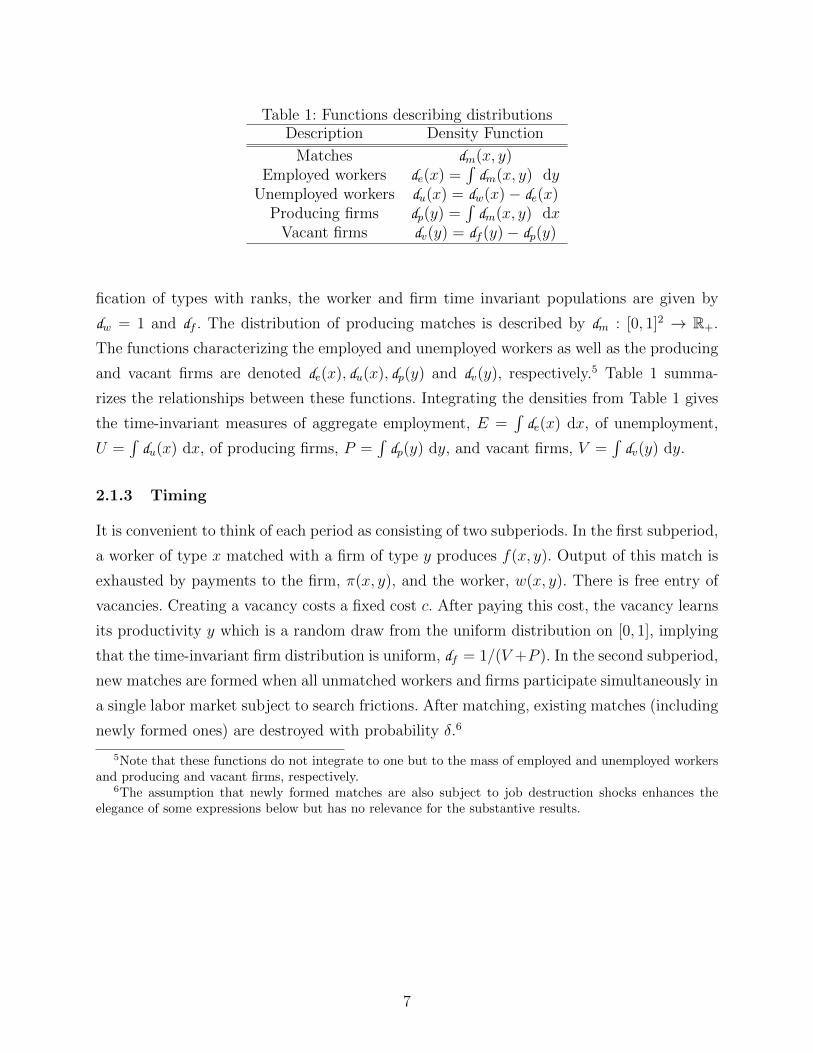
Table 1: Functions describing distributionsDescription Density Function
Matches dm(x, y)Employed workers de(x) =
∫dm(x, y) dy
Unemployed workers du(x) = dw(x)− de(x)Producing firms dp(y) =
∫dm(x, y) dx
Vacant firms dv(y) = df (y)− dp(y)
fication of types with ranks, the worker and firm time invariant populations are given by
dw = 1 and df . The distribution of producing matches is described by dm : [0, 1]2 → R+.
The functions characterizing the employed and unemployed workers as well as the producing
and vacant firms are denoted de(x), du(x), dp(y) and dv(y), respectively.5 Table 1 summa-
rizes the relationships between these functions. Integrating the densities from Table 1 gives
the time-invariant measures of aggregate employment, E =∫
de(x) dx, of unemployment,
U =∫
du(x) dx, of producing firms, P =∫
dp(y) dy, and vacant firms, V =∫
dv(y) dy.
2.1.3 Timing
It is convenient to think of each period as consisting of two subperiods. In the first subperiod,
a worker of type x matched with a firm of type y produces f(x, y). Output of this match is
exhausted by payments to the firm, π(x, y), and the worker, w(x, y). There is free entry of
vacancies. Creating a vacancy costs a fixed cost c. After paying this cost, the vacancy learns
its productivity y which is a random draw from the uniform distribution on [0, 1], implying
that the time-invariant firm distribution is uniform, df = 1/(V +P ). In the second subperiod,
new matches are formed when all unmatched workers and firms participate simultaneously in
a single labor market subject to search frictions. After matching, existing matches (including
newly formed ones) are destroyed with probability δ.6
5Note that these functions do not integrate to one but to the mass of employed and unemployed workersand producing and vacant firms, respectively.
6The assumption that newly formed matches are also subject to job destruction shocks enhances theelegance of some expressions below but has no relevance for the substantive results.
7

2.2 Search and Matching
Only and all unmatched agents engage in random search.7 A function m : [0, 1] × [0, 1] →[0,min(U, V )] takes the masses of unemployed workers U and vacant firms V as its inputs
and generates meetings. The probability a worker meets a potential employer is given by
Mu = m(U,V )U
, while the probability of a vacant firm meeting a potential hire is Mv = m(U,V )V
.
These probabilities are time-invariant in the steady-state equilibrium we will consider. The
probability for a worker to meet any firm y ∈ Y ⊆ [0, 1] equals Mu
∫Y dv(y) dy
V. The probability
for a firm to meet any worker x ∈ X ⊆ [0, 1] equals Mv
∫X du(x) dx
U. These probabilities
reflect our assumption of a linear search technology. Using the quadratic search technology
in Shimer and Smith (2000) these probabilities would be Mu
∫Y
dv(y) dy and Mv
∫X
du(x) dx,
respectively. Since we obtain the same search technology by simply setting U = V = 1 in
the matching process, it will become clear that our results do not depend on the returns to
scale of the matching function.
Not all meetings necessarily result in matches. Some meetings are between workers and
firms who are unwilling to consummate a match and who prefer to continue the search
process.
2.3 Strategies, Acceptance Sets and Surplus
The steady-state pure strategy of a worker of type x is to decide which firms to match
with, taking all other strategies as given. This strategy is described by a Borel measurable
acceptance set Aw(x) of firms that a worker type x is willing to match with. Symmetrically
for firms, the Borel measurable acceptance set Af (y) is comprised of the workers that a firm
of type y is willing to match with. Matching takes place when both the worker and the firm
find it mutually acceptable. For a worker of type x, the matching set Bw(x) consists of firms
which accept worker type x and are accepted by worker type x. Similarly, for a firm of type
y, Bf (y) consists of workers who accept to match with firm type y and who are accepted by
7Random search means that workers and firms do not observe the types of their potential trading partnersprior to meeting them, i.e. they have the same information as is available to the econometrician (e.g., age,sex, education, occupation, etc. of a worker and industry, location, etc. of a firm). An alternative assumptionis that workers (firms) know the type y of every firm (type x of every worker) and can direct their searchto specific types (e.g., Moen (1997), Shi (2001), Shimer (2005), Eeckhout and Kircher (2010)), e.g., workersdirect their search to firms that are willing to accept them. In the analysis below, these informationalassumptions matter only for the computation of the job filling probability for firms. These informationalassumptions will not affect the analysis at all if the data allow to observe the number of vacancies atindividual firms (as in, e.g., the German LIAB data that we use below). In this case one can compute the jobfilling rate directly without the need to make any informational assumptions. Without data on vacancies,the computation of the job filling rate is conditional on the specification of the matching process.
8
firms of type y. Specifically,
Bw(x) ≡ y : x ∈ Af (y) ∧ y ∈ Aw(x),
Bf (y) ≡ x : y ∈ Aw(x) ∧ x ∈ Af (y).
Bw and Bf denote the complements of Bw and Bf , respectively. Define B to represent all
(x, y) pairs that form in equilibrium:
B ≡ (x, y) : y ∈ Aw(x) ∧ x ∈ Af (y)
= (x, y) : y ∈ Bw(x)
= (x, y) : x ∈ Bf (y).
2.4 Bellman Equations and Surplus Sharing
Let Vu(x) denote the value of unemployment for a worker of type x, Ve(x, y) the value of
worker x employed at a firm of type y, Vv(y) the value of a vacancy for firm y, and Vp(x, y)
the value of firm y employing a worker of type x. The surplus of a match between worker x
and firm y is defined as
S(x, y) ≡ Vp(x, y)− Vv(y) + Ve(x, y)− Vu(x).
Shimer and Smith (2000) assume that wages are determined by Nash bargaining over
the match surplus S(x, y) between workers and firms who have equal bargaining powers.
We maintain this assumption in this paper, although it is not essential. First, we show
below that the assumption of equal bargaining powers can be relaxed and the bargaining
power can be identified in the data if the model incorporates either an idiosyncratic or an
aggregate stochastic component affecting, say, firm productivity. In terms of notation, we
allow for unequal bargaining powers by denoting workers’ bargaining power α ∈ (0, 1) (α = 12
corresponds to the model in Shimer and Smith (2000)). Second, our method for identifying
the sign and strength of sorting does not use the assumption of Nash bargaining but applies
to any bargaining game whose solution implies that payoffs to both parties increase in match
surplus. Finally, our method for the non-parametric identification of the production function
only relies on specifying the bargaining protocol which yields a wage equation that can be
inverted for output.
Generalized Nash bargaining over the match surplus with workers’ bargaining power α
9
implies
αS(x, y) = Ve(x, y)− Vu(x),
(1− α)S(x, y) = Vp(x, y)− Vv(y).
(1)
Following this rule, it is clear that y ∈ Aw(x) if and only if x ∈ Af (y). Hence,
Aw(x) = Bw(x) = y : S(x, y) ≥ 0,
Af (y) = Bf (y) = x : S(x, y) ≥ 0.
(2)
Using the surplus sharing rule (1), we obtain the following steady state value functions.
The derivations of these equations are provided in Appendix I.1.
Vu(x) = βVu(x) + βα(1− δ)Mu
∫Bw(x)
dv(y)
VS(x, y) dy, (3)
Vv(y) = βVv(y) + β(1− α)(1− δ)Mv
∫Bf (y)
du(x)
US(x, y) dx, (4)
Ve(x, y) = w(x, y) + βVu(x) + βα(1− δ)S(x, y), (5)
Vp(x, y) = f(x, y)− w(x, y) + βVv(y) + β(1− α)(1− δ)S(x, y). (6)
Free entry requires
c =
∫Vv(y)dy. (7)
2.5 Stationary Distribution of Matches
In the stationary match distribution, for all worker and firm type combinations in the match-
ing set the numbers of destroyed and created matches are the same:
∀(x, y) ∈ B δdm(x, y)︸ ︷︷ ︸destruction
= (1− δ)du(x)Mudv(y)
V︸ ︷︷ ︸new match formation
. (8)
The probability for a worker (of any type) to meet a firm of type y is the product of the
probability to meet any firm, Mu, and the probability that this firm is of type y, dv(y)V
. This
is multiplied by (1− δ) because newly formed matches can get destroyed in the same period.
Integrating over all matches yields that the total inflow into unemployment equals the total
10
outflow out of unemployment.∫Bδdm(x, y) dxdy = δE︸ ︷︷ ︸
inflow
= (1− δ)∫ 1
0
du(x)Mu
∫Bw(x)
dv(y)
Vdydx︸ ︷︷ ︸
outflow
.
2.6 Equilibrium
In a steady state search equilibrium (SE) all workers and firms maximize expected payoffs,
taking the strategies of all other agents as given.8 The economy is in steady-state. A SE is then
characterized by the density du(x) of unemployed workers, the density dv(y) of vacant firms,
the density of formed matches dm(x, y) and wages w(x, y). The density dm(x, y) implicitly
defines the matching sets as it is zero if no match is formed and is strictly positive if a match
is consummated. Wages are set to ensure the surplus sharing rule (1) and match formation
is optimal given wages w, i.e. a match is formed whenever the surplus is (weakly) positive
(see Eq. 2). The densities du(x) and dv(y) ensure that the flow equations in (8) hold.
To prove existence, Shimer and Smith (2000) assume that the production function is
either globally supermodular or globally submodular.9 A stronger assumption would be to
require that the production function induces either positive assortative matching (PAM) or
negative assortative matching (NAM), defined as follows:
Definition 1. Consider worker types x1 < x2 and firm types y1 < y2.
There is PAM if x1 ∈ Bf (y1) and x2 ∈ Bf (y2) whenever x1 ∈ Bf (y2) and x2 ∈ Bf (y1).
There is NAM if x1 ∈ Bf (y2) and x2 ∈ Bf (y1) whenever x1 ∈ Bf (y1) and x2 ∈ Bf (y2).
Whereas this stronger assumption is not necessary for the existence proof, it is commonly
imposed in the literature as we discuss below. The equilibrium existence proof in Shimer and
Smith (2000) also uses their assumption of a quadratic matching function. Noldeke and
Troger (2009) extend the proof to a linear matching technology used in this paper and show
that if f is either supermodular or submodular then a SE exists. Shimer and Smith (2000)
suggest that the assumption of either super or submodularity just avoids a more complicated
existence proof and thus can be dispensed with. More specifically, this assumption rules out
an atom of zero surplus matches, i.e.
∀x 6= x′ : µ(y : S(x, y) = S(x′, y) = 0) = 0, (9)
8As in Shimer and Smith (2000), we assume that a match is formed if agents are indifferent.9A production function is supermodular if the cross-derivative is positive and it is submodular if the
cross-derivative is negative.
11
where µ is the Lebesgue measure. Imposing
∀x 6= x′, ∀y : µ(y′ : f(x, y) + f(x′, y′) = f(x, y′) + f(x′, y)) = 0,
ensures this property. It thus avoids both the assumption of super or submodularity and also
a more complicated existence proof (see the Step 1 of the proof of Lemma 3 in Shimer and
Smith (2000)). This property is, for example, satisfied by the two production functions used
in Shimer and Smith (2000) as examples which satisfy neither PAM nor NAM: (x+ y)2 and
(x + y − 1)2. It does not hold for modular production functions such as x + y + k (k is a
constant). However for large enough k, every worker matches with every firm and thus (9)
is trivially satisfied. Thus, a SE exists.
3 The Econometric Model: Identification
The description of the econometric model requires to determine which variables are observ-
able and which are unobservable. The identity of a worker i and of a firm j are observed
but their respective types x(i) and y(j) are not. The wage is only observed with mean zero
measurement error εt, which is independent from all other variables, so that the observed
wage of a worker i employed at firm j equals
w(x(i), y(j)) + εi,j,t. (10)
All remaining variables or model primitives are unobserved.10
The model is (fully) identified if a unique function from the joint distribution of ob-
servables to (all) the underlying elements of the model exists. In particular, different model
primitives generate different joint distributions of observables, i.e. they are observationally
not equivalent.11 In this Section we establish that the model is identified by providing a
unique mapping from the joint distribution of wages, worker and firm identity to the primi-
tives of the model. The identification proof is constructive: We express the model parameters
in terms of the observable distribution and we also use these expressions to recover the prim-
itives of the model in the implementation in small samples. We proceed in three steps. First,
10In some data sets, such as the German LIAB data used in this paper, the number of vacancies v(j) postedby firm j is observed. Adding this to the lists of observables is not necessary but simplifies the measurement.
11This is the standard definition of identification in the literature building on Hurwicz (1950) (see Matzkin(2013) for a recent survey). As Matzkin (2013) explains, “The analysis of identification is separate from sta-tistical issues, which are dependent on sample size. Identification analysis assumes that the whole probabilitydistribution of the observable variables, rather than a sample from it, is available.”
12
we show how to identify the ranking of workers, that is the mapping x(i). Second, we identify
the ranking of firms, that is the mapping y(j). Having identified the rankings of workers and
firms, an investigation of the empirical matching patterns allows us to identify the presence
and sign of sorting. Third, we identify the remaining primitives of the model, in particular,
the output of every observed match between any worker and any firm.
Using the joint distribution of wages, workers and firms, we can infer the conditionally
expected wage
E(w(x(i), y(j)) + εi,j,t | i, j) = w(x(i), y(j)), (11)
since the measurement error has mean zero and is independently distributed. To prove iden-
tification we can therefore proceed under the assumption that we observe w(x(i), y(j)),
which is free of measurement error. Measurement error is, obviously however, a potential
impediment in small samples and we show how to deal with this issue successfully in the
implementation section below.
3.1 Ranking Workers
We now derive several statistics which are monotonically increasing in worker types. Such
statistics naturally provide a way to rank workers.
The easiest such statistic is the value of unemployment. It is increasing in a worker’s type
because a more productive worker can always imitate the acceptance strategy of the less
productive worker but produce more and consequently receive higher wages. This induces a
more productive worker to set a higher reservation wage. As the production function and the
value of unemployment increase in worker productivity, wages within firms are also increasing
in worker type. This yields for every firm a correct ranking of workers in the matching set of
that firm. If one firm were to match with all workers in the economy, the ranking of workers
based on wages in that firm would automatically represent a global ranking of all workers in
the economy. If no firm matches with all workers, we have to aggregate the partial within-firm
rankings to a global one. To illustrate how this works, consider a firm A which hires workers
a1 ≺ a2 ≺ . . . ≺ aN and another firm B which hires workers b1 ≺ b2 ≺ . . . ≺ bM where the
ranking within each firm is denoted by “≺”. Now suppose there is an overlap in the matching
sets of these two firms so that the best ranked workers in firm A are lowest ranked workers in
firm B, i.e. for some k, aN−k = b1, aN−k+1 = b2, . . . , aN = bk+1. We can then combine the two
rankings to rank all workers in the two firms to obtain a1 ≺ a2 ≺ . . . , aN−k = b1 ≺ aN−k+1 =
b2 ≺ . . . ≺ aN = bk+1 ≺ bk+2 ≺ . . . bM . Iterating yields a global ranking of workers under the
13
mild assumption that the set of workers can be split into overlapping matching sets. As the
matching sets cannot be guaranteed to be overlapping, we provide three further rankings -
the highest wage of a worker, the lowest wage of a worker, and the adjusted average wage -
which provide global rankings of workers.12 Thus, these ranking can be used to initialize the
rank aggregation procedure and this ensures a resulting global ranking even in cases with
non-overlapping matching sets.
Let ymin(x) be the firm that pays the lowest wage accepted by worker of type x and
ymax(x) be the firm that pays the highest wage to a worker of type x. In Appendix I we
prove:
Result 1. i) Vu(x), Ve(x, y) and w(x, y) are increasing in x.
ii) The lowest wage, given by w(x, ymin(x)), is increasing in x.
iii) The highest wage, given by w(x, ymax(x)), is increasing in x.
iv) The adjusted average wage, defined as
wav(x) ≡
1−Mu + δMu + Mu(1− δ)∫
Bw(x)
dv(y)
Vdy
w(x, ymin(x)) (12)
+ Mu(1− δ)∫
Bw(x)
dv(y)
Vw(x, y) dy,
is increasing in x.
Note that while the adjusted average wages is increasing in x, the average wage (without
the adjustment) is not.13 To see this, consider two workers with different productivities. A
more productive worker might be matching with a wider set of firms (some of which do
not accept the less able worker). However, the more able worker might be only marginally
acceptable to those firms because they typically match with even better workers. As a con-
sequence, those firms pay low wages to this worker. Thus, the average wage of the worker
12Flinn and Heckman (1982) and Wolpin (1987) represent some of the earliest work on order statisticestimators such as the lowest or highest wages.
13Since separation rates are identically δ at all firms a worker matches with, a worker’s average wage isproportional to
∫Bw(x)
w(x, y)dv(y) dy. Assuming, for simplicity, that Bw(x) = [ϕ(x), ϕ(x)], we get
∂
∂x
∫Bw(x)
w(x, y)dv(y) dy =
∫Bw(x)
∂w(x, y)
∂xdv(y) dy + ϕ′(x)w(x, ϕ(x))dv(ϕ(x))− ϕ′(x)w(x, ϕ(x))dv(ϕ(x)).
Clearly, this equation is not necessarily increasing in x.
14

over his employment history might be lower then that of a less productive worker. The more
productive worker still obtains higher utility because he spends a larger fraction of his life-
time employed. Result 1(4) corrects for this effect by imputing the value of unemployment
to unemployed workers and defining the average wage over the lifetime rather than of the
portion of lifetime the worker spends employed.
We have derived a number of statistics that provide theoretically valid and equivalent
rankings of workers. In Section 4 we discuss their implementation and assess their perfor-
mance in small samples and in the presence of measurement error in wages. We find that
the best way to rank workers is to use the global statistics to initialize the ranking and then
refine it by aggregating within-firm rankings. For a realistic amount of worker mobility across
firms this yields a very accurate complete ranking of workers.
3.2 Ranking Firms
To rank firms we derive a statistic which is monotonically increasing in firm type y.14 This is
non-trivial since the wage of worker x, w(x, y), is not always increasing in firm productivity.
The same problem applies to the surplus of a match, S(x, y). Our strategy is as follows. We
first establish that the value of a vacancy is increasing in y. This implies that the surplus
a vacancy is expected to generate is also increasing in y. Any bargaining game where both
parties benefit from an increase in the surplus implies that the average surplus of workers
employed by firm y is also increasing in y. Finally, we show that the average surplus of workers
employed by firm y can be expressed as a function of wages, yielding a simple observable
statistic that is increasing in y and thus allows to rank firms. In this Section, we include some
of the proofs in the main text as we consider them instructive (and surprisingly simple).
The foundation for our strategy of ranking firms is provided by the following result.
Result 2. Vv(y) and Vp(x, y) are increasing in y.
Our strategy is to relate these monotone statistics to observable statistics from the worker
side. The next result is stated only in terms of workers’ value functions.
Result 3. The expected surplus due to newly hired workers, given by
(1− δ)Mv
∫Bf (y)
du(x)
U(Ve(x, y)− Vu(x)) dx,
14Note that firms cannot be ordered based on data on average profits. This is because, just as averagewages do not necessarily increase in x, average profits are not necessarily increasing in y. In addition tothis theoretical obstacle, we are not aware of a convincing argument on how to overcome the well knowndifficulties in measuring profits in the data in a way consistent with the model.
15
is increasing in y.
Proof of Result 3. Using Eq. (1),
(1− δ)Mv
∫Bf (y)
du(x)
U(Ve(x, y)− Vu(x)) dx = α(1− δ)Mv
∫Bf (y)
du(x)
US(x, y) dx.
From (4), it follows that
Vv(y)(1− β)
β(1− α)= (1− δ)Mv
∫Bf (y)
du(x)
US(x, y) dx. (13)
From Result 2, both sides of (13) are increasing in y. Multiplying both sides of (13) by α
yields the desired result.
The proof used that the value of a vacancy is increasing in firm type y and then in-
volved two steps. First, since the value of a vacancy is related to the expected surplus by
an accounting identity (Eq. 4), the expected surplus is also increasing in firm type (Eq. 13).
The next step uses that Nash-bargaining implies that both the worker and the firm benefit
from an increase in the surplus. Nash bargaining has an even stronger implication as the
two parties benefit from an increase in the surplus in fixed proportions, determined by the
bargaining power. This strong implication is however not used here and our results extend
to other bargaining games where both parties benefit from an increase in the surplus.
Next, we relate this statistic to wages which are observable in the data.
Result 4. The expected wage premium over the reservation wage of newly hired workers,
given by
Ω(y) = (1− δ)Mv
∫Bf (y)
du(x)
U(w(x, y)− w(x, ymin(x))) dx, (14)
is increasing in y.
Note that this expectation is taken when the vacancy is still unfilled. The proof uses three
simple insights. Recall that w(x, ymin(x)) denotes the lowest wage (the reservation wage) that
worker x receives and ymin(x) is the firm type that pays this wage. The first insight is that
16
the lowest wage is equal to the return of being unemployed,15
w(x, ymin(x)) = (1− β)Vu(x) = (1− β)Ve(x, ymin(x)).
Second, the wage of a worker is a premium over the reservation wage (see Eq. 5),
w(x, y) = (1− β)Vu(x) + (1− β(1− δ)) (Ve(x, y)− Vu(x))
= w(x, ymin(x)) + (1− β(1− δ)) (Ve(x, y)− Vu(x)) .
Finally, this implies that the worker’s surplus is proportional to the difference between the
wage and the reservation wage,
w(x, y)− w(x, ymin(x)) = (1− β(1− δ))(Ve(x, y)− Ve(x, ymin(x))
).
Using Result 3 completes the proof.16
It is convenient to decompose Ω(y) into two factors that, as we show below, can be easily
measured in the data. The first is the average wage premium of newly hired workers at firm
y, Ωe(y), and the second one is the probability to fill a vacancy, q(y). The average wage
premium equals
Ωe(y) =
∫Bf (y)
du(x)U
(w(x, y)− w(x, ymin(x)))∫Bf (y)
du(x)U
dxdx. (15)
The probability that a vacancy of type y is filled equals
q(y) = (1− δ)Mv
∫Bf (y)
du(x)
Udx. (16)
15If a worker of type x is accepted by all firms, the lowest wage w(x, ymin(x)) is not equal to the reservationwage and thus not equal to the return of being unemployed. In Appendix I.3 we show that this does notchange the derivative of Ω. In particular, Ω is increasing in y independently from the properties of thematching set.
16The strict monotonicity of Ω and thus the ranking of firms depends on V (y) being increasing in y, asshown in Result 2. This result can be tested in the data using, e.g., the monotonicity test by Hall andHeckman (2000) which we describe and apply in Hagedorn et al. (2014) to discriminate between modelswith comparative and absolute advantage. In the empirical analysis below we indeed reject the constantΩ hypothesis, which is perhaps not surprising in view of the large firm heterogeneity documented by, e.g.,Bagger et al. (2011).
17
It then holds that
Ω(y) = q(y)Ωe(y). (17)
Computing Ωe(y) requires knowing workers’ reservation wages. While the reservation wage
is clearly conceptually related to the lowest accepted wage by a worker (which is observable
in the data), a more sophisticated measurement procedure is required in small samples and
in the presence of measurement error. We develop such a procedure in Section 4. We also
discuss the computation of the job filling rates q(y) in Section 3.4.3 below.
3.3 Sign and Strength of Sorting
Having ranked workers and firms, we can compute Spearman’s rank correlation between
x and y in the data, which is just the Pearson correlation coefficient since both types are
already ranked. The sign of this correlation is a natural indicator of the sign of sorting.
For example, a value of 1 indicates perfect positive assortative matching and a value of −1
indicates perfect negative assortative matching.
3.3.1 Relationship to the Literature
Note that Ω(y) is increasing in y regardless of whether the model features positive or negative
assortative matching, or indeed neither. In particular, it does not require any assumptions on
the production function f , i.e. neither super- nor sub-modularity. Because of this, Result 4
enables us to identify the sign of sorting. This is in contrast to the recent results of Eeckhout
and Kircher (2011) who used a simplified version of Atakan (2006) to show that the sign of
sorting cannot be identified from wage data. More precisely, they demonstrate that in their
two period model, for every supermodular production function that induces PAM there
exists a submodular production function that induces NAM and generates identical wages.
In Eeckhout and Kircher’s model workers and firms meet randomly in the first period. They
can either form a match or pay a search cost and be paired up with their ideal partners in a
perfectly competitive labor market in the second period. There is no discounting between the
two periods. These specific modeling choices simplify the theoretical analysis substantially,
but, unfortunately, they also ultimately prevent the identification of the model.
Consider first the role of discounting. One difference between Shimer and Smith (2000)
and the models in Atakan (2006) and Eeckhout and Kircher (2011) is that the former uses
discounting whereas search cost are explicit (and additive) in the latter two papers (as in
18
Chade (2001)). This matters for ranking firms, as can be seen by rearranging the Bellman
Equation (4) in our model:
Vv(y)(1− β) = β(1− α)(1− δ)Mv
∫Bf (y)
du(x)US(x, y) dx.
In the limit β → 1 we get that the expected surplus is a constant,
0 = (1− α)(1− δ)Mv
∫Bf (y)
du(x)
US(x, y) dx,
the Constant Surplus Condition in Theorem 1 in Atakan (2006). If, instead, β < 1, then
Vv(y)(1−β) is increasing in y and so is the expected surplus. This monotonicity (independent
of the production function) of expected surplus is the key step in our ranking of firms. We
then measure the surplus as being proportional to the wage premium of a worker resulting in
our statistic Ω(y) that is expressed in terms of wages only. Constructing the same statistic in
Atakan (2006) does not yield a function that is monotonically increasing in y but is, instead,
a constant. The impossibility to rank firms in Atakan (2006) is thus due to the knife-edge
assumption of no discounting. As soon as this assumption is relaxed, firms can be ranked.17
However, introducing discounting is not sufficient to achieve identification in Eeckhout
and Kircher (2011) due to further simplification they make relative to Atakan (2006). In
particular, their assumption of a frictionless second period matching implies that it is the
frictionless second period outcome π∗(y) that serves as the continuation value for firms, i.e.
the value of a vacancy equals
V (y) =
∫S(x, y)dx︸ ︷︷ ︸
expected surplus
+βπ∗(y).
Our statistic Ω(y) is monotone in y if and only if the expected surplus is. In Shimer and
Smith (2000) we show that this is the case because the value of a vacancy is increasing in y.
In Eeckhout and Kircher (2011) such a simple relationship between the value of a vacancy
and the expected surplus does not exist. Solving the above equation for the expected surplus
17Eeckhout and Kircher (2011) note that their non-identification proof breaks down in case of discounting.While this does not imply the possibility of identification, they conjecture that if one could somehow establishidentification, it might be difficult to achieve in practice for plausible values of β. The strength of our methodis that it is immune to such concerns. The statistic we use to rank firms is monotonically increasing in firmtype regardless of how close β is to one. In terms of the quantitative results reported below, we will show inAppendix VI.5 that even using the monthly discount factor as high as 0.999 does not measurably affect ourability to identify the objects of interest.
19
yields ∫S(x, y)dx = V (y)− βπ∗(y),
which is not necessarily increasing in y even with β 6= 1 since π∗(y) is increasing in y and
enters with a negative sign. As a result, our statistic Ω(y) which is proportional to expected
surplus is not necessarily monotonically increasing. Thus, the model in Eeckhout and Kircher
(2011) is not identified due to the assumption that the continuation value is the frictionless
allocation and not the value of a vacancy as in Shimer and Smith (2000) and in Atakan
(2006).
3.4 Identifying Remaining Model Parameters
We now show how to identify the remaining objects in the model. Our primary interest is
in identifying the production function f(x, y). We recover it, at the end of this section, by
inverting the wage equation. To accomplish that, we require the measures of the value of
unemployment Vu(x), the value of a vacancy Vv(y), and the probability to fill a vacancy q(y).
Alongside with measuring these key objects, we also show how to measure the value of being
employed Ve(x, y), the value of producing for a firm Vp(x, y), and the meeting probabilities
for unemployed workers and vacant firms Mu and Mv.
3.4.1 Measuring Vu(x), Ve(x, y), and S(x, y)
The Bellman Equation (5), implies, using Ve(x, ymin(x)) = Vu(x), that Vu(x)(1 − β) =
w(x, ymin(x)). Thus, the reservation wage for workers of type x can be used to measure the
(type-dependent) value of unemployment as18
Vu(x) =w(x, ymin(x))
1− β.
To measure Ve(x, y), consider a worker of type x, who starts working at a firm of type
18Implementation of the measurement of (type-dependent) reservation wages is described in Section 4.3.Alternatively one can, e.g. if no firm pays exactly the reservation wage, compute the value of unemploymentusing equations (3) and (5) as:
Vu(x) =
β(1−δ)Mu
1−β(1−δ)∫
Bw(x)
dv(y)V w(x, y) dy
(1− β)(1 + β(1−δ)Mu
1−β(1−δ) )∫
Bw(x)
dv(y)V dy.
20

y at time t = 0, becomes unemployed at time tU , and receives wage wt = w(x, y) for all t
between t = 0 and t = tU − 1. We then define
tU−1∑t=0
βtwt + βtUVu(x),
where, of course, we use the measured value for Vu(x). Averaging across all these sums for
all types x starting at firm y yields the estimate Ve(x, y).
We then also have a measure of surplus multiplied by the bargaining power
αS(x, y) = Ve(x, y)− Vu(x).
Using that α = 12
in the model of Shimer and Smith (2000), yields the value of S(x, y).
In Appendix I.4 we follow Hagedorn and Manovskii (2008, 2013) and describe how the
parameter α can be identified from the data in a more general version of the model.
3.4.2 Measuring Vv(y) and Vp(x, y)
We next turn to the measurement of Vv(y), which is related to our estimate Ω(y) through
Vv(y)(1− β) = β1− αα
(1− δ)Ω(y).
Since, as discussed above, we can measures Ω in the data, and we can follow the standard
approaches in the literature to estimate or calibrate δ and β, we obtain
Vv(y) =β
1− β1− αα
(1− δ)Ω(y).
Using this, Vp(x, y) can then be computed from
Vp(x, y) = Vv(y) + (1− α)S(x, y).
3.4.3 Transition Rates
The probability, q(y), that a vacancy posted by firm j of type y(j) is filled conditional on
meeting a worker is simply the share of unemployed workers belonging to this firm’s matching
set in total unemployment. Indexing workers by their (estimated) rank x, denote by u(x)
21
this type’s average unemployment rate. Using the law of large numbers, it holds that
q(y) ≡∫
Bf (y)
du(x)
Udx =
∫Bf (y)
u(x) dx∫[0,1]
u(x) dx. (18)
Note that q(y) can be computed in the data and that its knowledge is sufficient to rank
firms as q(y) is proportional to q(y) (see Eq. 16). Next, we measure Mv. Denote by Ht(y)
the observed number of new hires in firms of type y at time t, and by Vt(y) the unobserved
number of vacancies posted by these firms. Eq. (16) and the law of large numbers imply that
Ht(y)
(1− δ)q(y)= MvVt(y).
Adding up across all firms and time periods, and rearranging yields Mv (and Mu as MuU =
MvV ):
Mv =1
1− δ
∫[0,1]
Ht(y)q(y)
dy∫[0,1]
Vt(y) dy,
where∫
[0,1]Vt(y) dy is the total number of vacancies, which if unobserved, can be inferred
by matching the wage share in output.
These computations simplify if data on firm-level vacancies are available.19 In this case
we can directly measure the probability to fill a vacancy q(y). For every worker type we can
measure the probability to leave unemployment λ(x). With firm level vacancy data (i.e. data
for dv(y)), we can then measure Mu (and consequently Mv) from
λ(x) = (1− δ)Mu
∫Bw(x)
dv(y)
Vdy.
A more robust way is to integrate over all worker types and solve for Mu from∫ 1
0
λ(x) dx = (1− δ)Mu
∫ 1
0
∫Bw(x)
dv(y)
Vdydx.
19The computation is also not affected if there is random noise leading to observing some firms hiringwithout having a posted vacancy.
22
3.4.4 Measuring output f(x, y)
Using the equation for wages (A2), the production function f(x, y) on the set of matches
that actually form, then equals
f(x, y) =w(x, y)− α(β − 1)Vv(y)− (1− α)(1− β)Vu(x)
α.
The output of a match is determined by inverting the wage equation, expressing the output
f(x, y) as a function of the observed wage w(x, y) and the two measured outside options
Vv(y) and Vu(x). For this to be feasible the researcher has to know the exact wage equation.
In the model of Shimer and Smith (2000) this is the case since Nash bargaining is imposed.
Other wage determination mechanisms which imply an invertible wage equation would also
allow for an identification of output.
An alternative strategy for recovering the output is to invert the equation for surplus
(A1). As S(x, y), Vv(y) and Vu(x) have already been measured, this immediately implies
f(x, y).
4 Implementation and Quantitative Evaluation
In this section we develop the key implementation steps of the proposed identification strat-
egy and evaluate their performance in a Monte Carlo study over a range of parameter values
that are likely to be encountered in empirical work. As our identification proof is fully con-
structive, the only challenge is to deal with the fact that available data sets are finite whereas
theoretical identification assumes infinite data. This is particularly relevant to estimating
a worker’s reservation wage which can only be imprecisely estimated from an individual
worker’s few own wage observations. To obtain precise estimates, we propose an ostensibly
simple but indeed very effective methodological innovation. After workers have been ranked,
we bin similarly ranked workers. Given the large number of workers in available data sets,
closely ranked workers are very similar. We then use wage observations for all workers in
this bin as if they were a single worker’s observations and compute the relevant statistics
accordingly. Analogously, we also bin firms after they have been ranked to compute statistics
for a single firm using the observations for all firms in the respective bin. In Monte-Carlo
simulations we find that binning workers and firms is the key to precisely recovering all model
primitives in the data.20 We now describe the key steps of our implementation strategy, with
20Krasnokutskaya et al. (2014, 2016) pursue a similar approach in the context of online auctions wherethey group bidders on the basis of their quality.
23
the detailed implementation algorithm provided in Appendix II.
4.1 Parameterization
We assume that a researcher has access to a matched employer-employee panel data set with
a time dimension of 20 years. Most currently available and commonly used matched data
sets (e.g., from Brazil, Denmark, Germany, France) have a similar or longer time span. We
assume that the data include the information on wages, all employment and unemployment
spells of the worker over the duration of the sample, and all hires and separations at the firm
level. We simulate the model at a monthly frequency. The production functions commonly
used in the literature belong to the constant elasticity of substitution (CES) family. We
consider three such function:
i) f(x, y) = 0.6 + 0.4(x1/2 + y1/2)2, which induces positive assortative matching (PAM),
ii) f(x, y) = (x2 + 2y2)1/2, which induces negative assortative matching (NAM), and
iii) f(x, y) = 0.4 + 1x≤0.4(x+ 0.6)y + 1x>0.4 ((x− 0.4)2 + y2)1/2
, which induces neither
positive nor negative assortative matching (NEITHER). Instead, the pattern of sorting
changes over its domain (PAM for x ≤ 0.4 and NAM for x > 0.4).
The literature has largely restricted attention to identifying sorting assuming that the
production function induces either globally positive or negative assortative matching. This
motivates our choice of the first two production functions. Our method, however, does not
rely on placing such restrictions. The choice of the third production function is designed to
illustrate this point. The production functions are scaled to generate a realistic amount of
wage dispersion.
We also consider three distributions of workers and firms (these are the “original” non-
rank distributions F and G). Common choices in the literature are either a uniform or normal
distributions. We consider both and for the normal distribution we choose the mean of 0.5
and the variance of 0.25 (the distribution is truncated and normalized on [0, 1] interval). We
also consider a bimodal distribution constructed as the sum of two normals: N(0.2, 0.25) +
N(0.8, 0.25) truncated and normalized to integrate to one on [0, 1]. The distributions are
discretized into 50 values on an evenly spaced grid. We simulate a small sample of 30,000
workers. The vacancy creation cost is such that there is the same number of jobs in the
economy. After the productivity of the vacancies is learned, vacancy creators sell them in
competitive markets to operating firms with the same productivity level. We use 300 firms
24

Table 2: Parameterizations
Parameter Symbol Option 1 Option 2 Option 3Production function f(x, y) PAM NAM NEITHERWorker distribution dw Uniform Normal Bi-ModalFirm distribution df Uniform Normal Bi-ModalDiscount factor β 0.996Separation rate δ 0.01 0.025Meeting function scale κ 0.4 0.7Meeting function elasticity ν 0.5Worker’s bargaining weight α 0.5Measurement error in wages ε 20% of overall wage variance
in simulations, which implies in a symmetric equilibrium that operating firms have 100 jobs
per firm (all sharing the same productivity level). As not all of these jobs are filled at a point
in time, the actual size of employment at each firm varies across parameterizations but is
not more than 100 workers. We set the discount factor to 0.996 at monthly frequency to be
consistent with the annual interest rate of 4%.
We assume the standard Cobb-Douglas form of the meeting function m(s, v) = κsνv(1−ν).
We set the elasticity parameter ν = 0.5 as this parameter plays no interesting role in our
stationary model. We consider a wide range for the scale parameter κ = 0.4, 0.7 to generate
job finding probabilities ranging between a high of about 50% a month in the US and a low
of about 15% in some European countries. Similarly, we choose two values for the separation
rate δ = 0.01, 0.025, roughly spanning the US and European evidence. Bargaining weights
of 0.5 are symmetric for workers and firms.
Finally, we allow for measurement error in wages. Hagedorn and Manovskii (2012) es-
timate that measurement error accounts for approximately 20% of the variance of residual
wages in the US NLSY data. This is likely an upper bound on the matched employer-employee
data sets as these data are typically based on administrative sources with highly reliable wage
information. Nevertheless, to make the test of the proposed method more stringent, we add
iid noise to every wage observation with a variance of 20% of the correctly measured wage
variance. The error is simulated as draws from a normal distribution truncated at three
standard deviations around the mean of zero.
The values of parameters used in simulations are summarized in Table 2. All combinations
of parameters result in 108 distinct parameterizations. Appendix Figure A-3 summarizes the
values that a number of variables of interest take across all parameterizations. Most tend to
lie within empirically plausible ranges.
25
0.96 0.965 0.97 0.975 0.98 0.985 0.99 0.995 10
10
20
30
40
50
60
70
80
Correlation
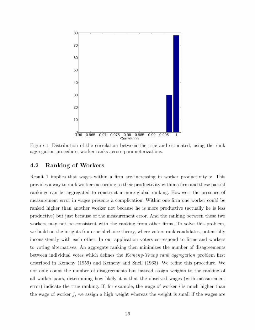
Figure 1: Distribution of the correlation between the true and estimated, using the rankaggregation procedure, worker ranks across parameterizations.
4.2 Ranking of Workers
Result 1 implies that wages within a firm are increasing in worker productivity x. This
provides a way to rank workers according to their productivity within a firm and these partial
rankings can be aggregated to construct a more global ranking. However, the presence of
measurement error in wages presents a complication. Within one firm one worker could be
ranked higher than another worker not because he is more productive (actually he is less
productive) but just because of the measurement error. And the ranking between these two
workers may not be consistent with the ranking from other firms. To solve this problem,
we build on the insights from social choice theory, where voters rank candidates, potentially
inconsistently with each other. In our application voters correspond to firms and workers
to voting alternatives. An aggregate ranking then minimizes the number of disagreements
between individual votes which defines the Kemeny-Young rank aggregation problem first
described in Kemeny (1959) and Kemeny and Snell (1963). We refine this procedure. We
not only count the number of disagreements but instead assign weights to the ranking of
all worker pairs, determining how likely it is that the observed wages (with measurement
error) indicate the true ranking. If, for example, the wage of worker i is much higher than
the wage of worker j, we assign a high weight whereas the weight is small if the wages are
26

very similar. We use a Bayesian approach to compute these weights. The goal is then to find
a ranking that maximizes the sum of weights in favor of a proposed ranking. To deal with
the computational complexity of this problem, we build on insights from Kenyon-Mathieu
and Schudy (2007) who provide a polynomial time algorithm that approximates the solution
to this problem with arbitrary degree of accuracy. In practice, we found that implementing
a portion of their algorithm achieves a high level accuracy while being quite fast. A detailed
description is provided in Appendix III.
Figure 1 reports the distribution of the rank correlations of the true worker types and
types recovered using the rank aggregation procedure across simulations. The results indicate
that the procedure recovers the correct rankings quite well despite relatively small samples
and in the presence of sizable measurement error in wages.21
4.3 Ranking of Firms
Result 4 implies that to rank firms one simply needs to compute the expected average
difference between the wages a firm pays to each of its newly hired workers and the reservation
wage of those workers. The only challenge is to obtain an accurate estimate of the reservation
wage for each worker, despite the limited time dimension of the available data. The key
insight we use is that once workers are ranked, similarly ranked workers must have similar
reservation wages. Thus, we can estimate the reservation wage by considering a group of
similar workers, despite the fact that each of those workers is observed for a relatively short
period of time. Since workers are ranked and ranks are uniformly distributed, we can group
workers into bins of equal size. One can think of workers as ordered on a line and bins
corresponding to intervals (without holes) on this line. What remains to be determined is
the number of bins or equivalently the size of the bin. The answer to this question obviously
depends on the size of the sample. If we had infinite observations for each worker the choice
would be easy as each bin would consist of one worker only as these infinite observations
are sufficient to compute the worker’s reservation wage from this worker’s observed wages
only. However, we only have a small sample available and the appropriate bin size has to be
evaluated in Monte-Carlo simulations. In these simulations we find that 50 bins are sufficient
to reliably compute all statistics, such as the reservation wage and the production function.
21As implied by Result 1, we initialize the rank aggregation procedure using global rankings based onthe lowest accepted wage, the highest accepted wage, or the adjusted average wage. The performance ofeach of these methods is reported in Appendix Figure A-4. The correlations are relatively high for all thesemeasures. In particular, the adjusted average wage dominates both the minimum and the maximum wage inits performance in ranking workers. The measure based on rank aggregation substantially outperforms anyof the individual measures.
27
0.97 0.975 0.98 0.985 0.99 0.995 10
5
10
15
20
25
30
35
40
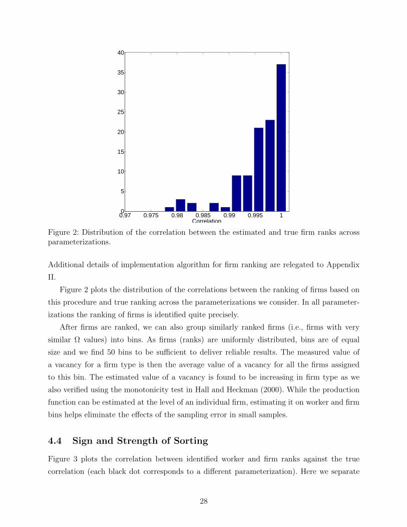
Correlation
Figure 2: Distribution of the correlation between the estimated and true firm ranks acrossparameterizations.
Additional details of implementation algorithm for firm ranking are relegated to Appendix
II.
Figure 2 plots the distribution of the correlations between the ranking of firms based on
this procedure and true ranking across the parameterizations we consider. In all parameter-
izations the ranking of firms is identified quite precisely.
After firms are ranked, we can also group similarly ranked firms (i.e., firms with very
similar Ω values) into bins. As firms (ranks) are uniformly distributed, bins are of equal
size and we find 50 bins to be sufficient to deliver reliable results. The measured value of
a vacancy for a firm type is then the average value of a vacancy for all the firms assigned
to this bin. The estimated value of a vacancy is found to be increasing in firm type as we
also verified using the monotonicity test in Hall and Heckman (2000). While the production
function can be estimated at the level of an individual firm, estimating it on worker and firm
bins helps eliminate the effects of the sampling error in small samples.
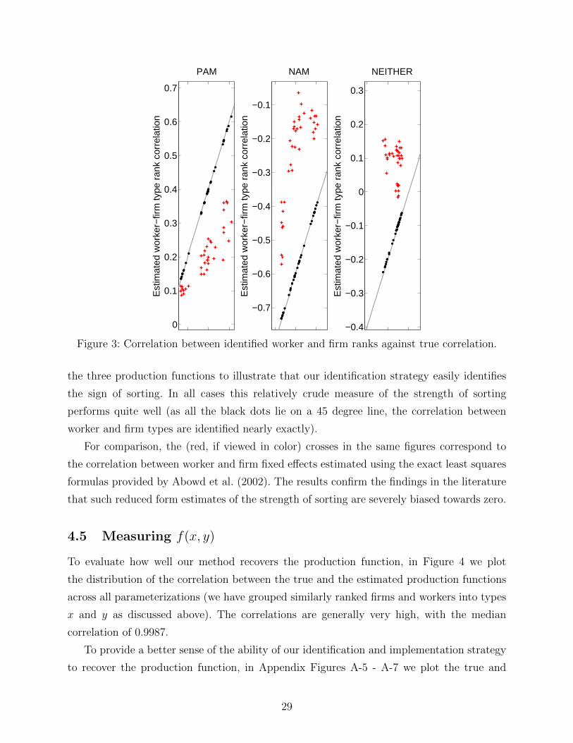
4.4 Sign and Strength of Sorting
Figure 3 plots the correlation between identified worker and firm ranks against the true
correlation (each black dot corresponds to a different parameterization). Here we separate
28
0.2 0.4 0.60
0.1
0.2
0.3
0.4
0.5
0.6
0.7
Est
imat
ed w
orke
r−fir
m ty
pe r
ank
corr
elat
ion
PAM
−0.8 −0.6 −0.4
−0.7
−0.6
−0.5
−0.4
−0.3
−0.2
−0.1
Est
imat
ed w
orke
r−fir
m ty
pe r
ank
corr
elat
ion
NAM
−0.4 −0.2 0−0.4
−0.3
−0.2
−0.1
0
0.1
0.2
0.3
Est
imat
ed w
orke
r−fir
m ty
pe r
ank
corr
elat
ion
NEITHER
Figure 3: Correlation between identified worker and firm ranks against true correlation.
the three production functions to illustrate that our identification strategy easily identifies
the sign of sorting. In all cases this relatively crude measure of the strength of sorting
performs quite well (as all the black dots lie on a 45 degree line, the correlation between
worker and firm types are identified nearly exactly).
For comparison, the (red, if viewed in color) crosses in the same figures correspond to
the correlation between worker and firm fixed effects estimated using the exact least squares
formulas provided by Abowd et al. (2002). The results confirm the findings in the literature
that such reduced form estimates of the strength of sorting are severely biased towards zero.
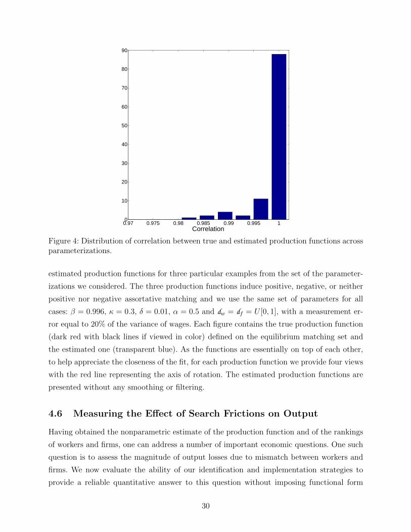
4.5 Measuring f(x, y)
To evaluate how well our method recovers the production function, in Figure 4 we plot
the distribution of the correlation between the true and the estimated production functions
across all parameterizations (we have grouped similarly ranked firms and workers into types
x and y as discussed above). The correlations are generally very high, with the median
correlation of 0.9987.
To provide a better sense of the ability of our identification and implementation strategy
to recover the production function, in Appendix Figures A-5 - A-7 we plot the true and
29
0.97 0.975 0.98 0.985 0.99 0.995 10
10
20
30
40
50
60
70
80
90
Correlation
Figure 4: Distribution of correlation between true and estimated production functions acrossparameterizations.
estimated production functions for three particular examples from the set of the parameter-
izations we considered. The three production functions induce positive, negative, or neither
positive nor negative assortative matching and we use the same set of parameters for all
cases: β = 0.996, κ = 0.3, δ = 0.01, α = 0.5 and dw = df = U [0, 1], with a measurement er-
ror equal to 20% of the variance of wages. Each figure contains the true production function
(dark red with black lines if viewed in color) defined on the equilibrium matching set and
the estimated one (transparent blue). As the functions are essentially on top of each other,
to help appreciate the closeness of the fit, for each production function we provide four views
with the red line representing the axis of rotation. The estimated production functions are
presented without any smoothing or filtering.
4.6 Measuring the Effect of Search Frictions on Output
Having obtained the nonparametric estimate of the production function and of the rankings
of workers and firms, one can address a number of important economic questions. One such
question is to assess the magnitude of output losses due to mismatch between workers and
firms. We now evaluate the ability of our identification and implementation strategies to
provide a reliable quantitative answer to this question without imposing functional form
30
assumptions on technology.22
To do so we first derive the (counterfactual) allocation in a world without frictions. To
solve for the frictionless assignment we need to find a one-to-one assignment (bijection)
µ : [0, 1]→ [0, 1] of workers to firms such that the total output∑
x f(x, µ(x)) is maximized.
Our identification strategy identifies the production function only on the set of (x, y) matches
observed in the data. Since our objective is to find an optimal assignment on this set, we
assume that the output outside of the observed frictional matching set is zero.
This assignment problem is a well studied combinatorial optimization problem and there
are several existing algorithms that can solve it in polynomial time.23 However, a complete
solution is not required to approximate the effect of the elimination of search frictions on
output. Instead, a much smaller scale assignment problem can be solved on a random sample
of workers and firms. We choose the size of the sample so that the maximum total output of
the sample scaled to the size of the total population of workers and firms becomes invariant
to the sample size. Across our simulations, we found that a sample of about 5000 workers
and 5000 jobs is sufficient. On a sample of that size we can solve the problem in minutes
using the Jonker and Volgenant (1987) algorithm without special hardware.
Denote by Eno fric the expectation of frictionless output f(·, µ(·)):
Eno fric =
∫ 1
0
f(x, µ(x)) dx, (19)
where we used that worker ranks are uniformly distributed. In the presence of frictions, let
Efric be the expectation of f :
Efric =
∫Bf(x, y)dm(x, y) dxdy. (20)
Then, the output loss due to misallocation is the difference between the expected output
22An alternative approach to measuring the cost of mismatch was pursued by Eeckhout and Kircher (2011).They noted (as did Gautier and Teulings 2004, 2006) that differentiating the wage equation (such as Eq. A2in this paper) the cross-partial derivative of the wage equals the cross-partial derivative of the productionfunction multiplied by the worker bargaining weight. They also show that in their two period model, wherea period with search frictions is followed by a frictionless period and there is no discounting, and underthe assumption that the production function globally induces PAM or NAM, the average cross-partial ofthe production function can be theoretically related to the output cost of mismatch. They do not explorethe empirical properties of this estimator given the nature of the available data. Even maintaining theirrestrictive assumptions on the production technology, it is not clear whether it is possible to generalize thismethod to the fully dynamic model in Shimer and Smith (2000).
23See Burkard et al. (2009) for a review.
31

4 5 6 7 8 9 10 11 12
4
5
6
7
8
9
10
11
12
True Output Percent Gain
Est
imat
ed O
utpu
t Per
cent
Gai
n
0.5% Bound
(a) Eliminating frictional unemployment.
1 1.5 2 2.5 3
1
1.5
2
2.5
3
True Output Percent Gain
Est
imat
ed O
utpu
t Per
cent
Gai
n
0.5% Bound
(b) Keeping frictional employment level.
Figure 5: Estimated gains from eliminating frictions.
without frictions, Eno fric and the expected output with frictions, Efric:
∆E = Eno fric − Efric. (21)
In Figure 5, we plot the percent output gain from the optimal reallocation of workers
100· ∆E
Efric . The true output gain as a percent of frictional output is on the horizontal axis while
the estimated gain as a percent of frictional output is on the vertical axis. To help visually
interpret the results, the figure also includes two dotted lines that represent a mistake of plus
or minus one half of one percent of output. In Panel 5(a) we plot the estimated gains from
eliminating all frictions, including the elimination of frictional unemployment. In Panel 5(b)
we only consider the effect from optimal reassignment of workers employed in the economy
with frictions (that is, we keep the employment of each worker type fixed at its level in the
economy with frictions).24 We interpret the results as indicating that the method performs
quite well in estimating the gain from optimal worker reallocation.25
24The relatively small gains from reallocation in this experiment are driven by the parsimonious CESproduction function. Larger gains from eliminating mismatch can be obtained with more cumbersome spec-ifications of the production functions. We have explored a number of such specifications and found that ourmethod continues to perform equally well.
25Note that the high correlations between the true and estimated production functions reported in Figure4 do not necessarily imply an accurate estimate of the gains from optimal assignment. The reason is that thesolution to the optimal assignment problem exploits all imperfections of the estimated production function.Thus, it is possible to have a high correlation of the true and estimated production function and to substan-tially miss on the estimated gains from reallocation. The good fit of Figure 5 implies that our methodologydoes not introduce such significant exploitable imperfections.
32

4.7 Robustness
In this section we conduct several robustness checks. First we allow for a shorter time horizon
and assume that data are available only for 10 years. Second, we look at smaller firms and
third, we allow for random match-specific productivity.
4.7.1 Shorter Time Horizon
In the quantitative evaluation we assumed - guided by the available matched employer-
employee data sets - that we have data for 20 years. We now investigate how the results
change if we have only a shorter data set of 10 years available, which may be the case for
some developing countries or if an estimation on subsamples of available data is considered.
We find that the quantitative performance of our method is not substantially affected by this
restriction. Results reported in Appendix VI.2 imply that when using only 10 years of data
the median correlation between the true and the estimated production function is 0.9972,
the correlation between the firm and the worker ranking is very well recovered and so are
the gains from eliminating search frictions.
4.7.2 Small Firms
In the benchmark, the maximum potential size of the firm, that is the sum of employment and
vacancies, was set to 100. Results reported in Appendix VI.3 suggest that the quantitative
performance of the method does not worsen substantially if we instead restrict the maximum
potential firm size to 20 workers. In particular, we find that the median correlation between
the true and the estimated production function is 0.9962, the correlation between firm and
worker ranking is very well recovered and so are the estimated gains from eliminating search
frictions.
4.7.3 Match Quality
The Monte Carlo experiments reported above illustrate that our implementation strategy can
successfully overcome the effects of measurement error in wages. Another potential source
of noise in identification is idiosyncratic match productivity. When a worker of type x and
a firm of type y meet they draw, before deciding whether to produce together, a random
productivity realization z from a distribution Γ, so that production equals f(x, y)+z for the
duration of the match.
Thus, there are now two sources of match specific productivity. The first depends on the
fixed types x and y and the second one is z. Although z is a random draw from a distribution
33
that is independent of either x or y, the accepted value of z depends on the worker and firm
types. As a result a worker and a firm either do not produce at all or they start producing
for all realizations of match quality above some threshold level z(x, y).
Using this model, we repeat the Monte Carlo study with the same parameterizations.
The choice of the offer distribution of match quality Γ is made consistent with the findings
in Low et al. (2010). These authors find that the variance of the offer distribution for match
quality Γ is about 0.22 of the variance of overall wages, where observables are removed.
As we have an equilibrium model where the wage of a worker is determined endogenously
given the production function, the “offer” distribution for output z is exogenous and not
the offer distribution for wages as in the partial equilibrium model in Low et al. (2010). In
particular changes in z in the production function do not necessarily translate one-to-one
into wage changes. We therefore pick the distribution Γ such that the endogenous wage offer
distribution in the model has the same variance as the exogenous wage offer distribution in
Low et al. (2010). The resulting median variance of Γ relative to the variance of wages in the
model equals 0.2085. Similarly, we use the estimates in Low et al. (2010) to set the variance
of measurement error relative to the variance of wages to 0.027. Thus, our identification
methodology is potentially complicated due to two sources of noise: idiosyncratic match pro-
ductivity and measurement error. In Appendix VI.4 we report that this is not quantitatively
important, however, by conducting the same experiments as in the benchmark and using the
same implementation strategy. We find that the median correlation between the true and the
estimated production function is 0.9961, the correlation between firm and worker ranking is
very well recovered and so are the estimated gains from eliminating search frictions.
We should point out that adding match productivity allows for an easy extension of our
methodology which renders it more powerful. As the support of the distribution of z is very
wide, there exist values of z that induce a match between many worker types and many firm
types. For example, we find that a match between a worker of type x and a firm of type
y that would not form for low realizations of match-specific productivity, will form if the
realization of z is sufficiently high. This implies that for each firm where some z’s but not all
are accepted by a worker of type x, the lowest wage paid by this firm to this worker is the
reservation wage of this worker. Given the wide support of z we find that for the majority
of firms the lowest wage paid is the reservation wage. Clearly, this makes the estimation of
the reservation wage much more precise.26
26We thank an anonymous referee for drawing our attention to this improvement of our methodology. Onecan use this insight to also recover the threshold acceptance level z(x, y) and thus also decompose the outputof a pair (x, y) into f(x, y) and the contribution from match quality.
34

5 Identification: Data
In this section we apply our methodology to a German matched employer-employee dataset
to identify all features of the model, in particular the ranking of workers, the ranking of firms
and the production function. A key feature of the data is a substantial movement of workers
between jobs without intervening unemployment spells. We therefore first extend the basic
model to include on-the-job search and then show that the identification and implementation
methodology extends from the basic model to the model with on-the-job search.
5.1 Model and Identification with On-the-Job Search
An unemployed worker makes a take-it-or-leave-it offer to a firm and thus extracts the full
surplus.27 As in Postel-Vinay and Robin (2002) and Cahuc et al. (2006), when a worker
employed at some firm y meets a firm y which generates higher surplus, the two firms engage
in Bertrand competition such that the worker moves to firm y and obtains the full surplus
generated with firm y. Small costs of writing an offer prevent firms y which generate lower
surplus than the current firm y from engaging in Bertrand competition. The remaining details
of the model description are delegated to Appendix IV.
We now show that all the theoretical results which established identification in the bench-
mark model continue to hold in our model with on-the-search and establish identification in
this model as well.
Ranking Workers. The following result establishes that wages within a firm rank workers
hired out of unemployment.
Result 5. Within a firm, wages of workers hired from unemployment are increasing in
worker type.
We can therefore use the same algorithm as in the benchmark model with the restriction
that it is applied to workers hired out of unemployment only. This reduces the number of
usable observations relative to the benchmark model, but we show in Appendix IV that this
reduction does not significantly worsen the performance of our methodology.
Ranking Firms. To rank firms we derived a statistic - the value of vacancy - which is
27This assumption is special but, as we will see below, the model based on this assumption provides avery tight fit to the data. Alternative assumptions may break some of the monotonicity properties on whichour identification strategy relies. Establishing identification of a more general model of on-the-job search isa promising avenue for future research.
35
monotonically increasing in firm type y and which can be expressed as a function of wages
observed in the data. The same result holds in the model with on-the-job search:
Result 6. The value of a vacancy Vv(y) is increasing in firm type y and can be expressed as
a function of wages.
We can therefore again use observable wages to rank firms in terms of their productivity.
The actual statistic is slightly different from the one in the benchmark model, but it is even
easier to implement as it does not involve estimating workers’ reservation wages.
Measuring output f(x, y). Finally we can also recover the output of every match from
inverting the wage equation, which relates output to observable variables.
Result 7. The wage equation can be inverted so that output can be expressed in terms of
observables.
5.2 Data Description
Our empirical analysis uses the model with on-the-job search and is based on the German
LIAB data set, which is the primary source of data used in the research on the contribution
of worker and firm effects to wage dispersion in Germany, e.g., Dustman et al. (2009). These
data, spanning the 1993-2007 period, represent the linked employer-employee data set of the
Institute for Employment Research (Institut fur Arbeitsmarkt- und Berufsforschung, IAB).
The LIAB combines the Employment Statistics of the German Federal Employment Agency
(Bundesagentur fur Arbeit) with establishment level data from the IAB Establishment Panel.
For detailed information on the LIAB, see Alda et al. (2005).
We follow Card et al. (2013) in selecting the sample and in constructing the residual wages
which form the basis of the analysis in both papers. The only adjustments we make are due to
the fact that, in the data we have access to, all workers employed at the establishments from
the representative IAB Establishment Panel can be observed, while we do not necessarily
observe all workers employed in other establishments. Card et al. (2013) have access to the
universe of workers and establishments. This does not limit our analysis as LIAB provides
us with complete continuous (up to a day) earnings and employment histories of workers
who worked in the establishments from the Establishment Panel for at least one day (even
when these workers are employed in other establishments). One potential advantage of using
the LIAB is that it contains information on vacancies at the establishment level which are
not available for firms outside the Establishment Panel. Descriptive statistics and additional
details are provided in Appendix V.
36
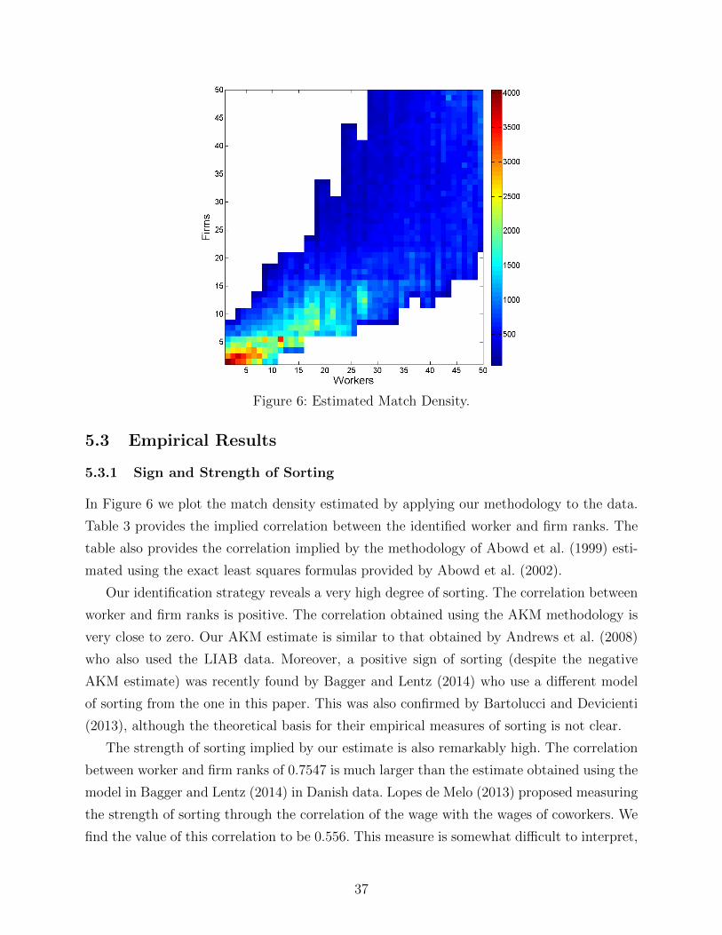
Figure 6: Estimated Match Density.
5.3 Empirical Results
5.3.1 Sign and Strength of Sorting
In Figure 6 we plot the match density estimated by applying our methodology to the data.
Table 3 provides the implied correlation between the identified worker and firm ranks. The
table also provides the correlation implied by the methodology of Abowd et al. (1999) esti-
mated using the exact least squares formulas provided by Abowd et al. (2002).
Our identification strategy reveals a very high degree of sorting. The correlation between
worker and firm ranks is positive. The correlation obtained using the AKM methodology is
very close to zero. Our AKM estimate is similar to that obtained by Andrews et al. (2008)
who also used the LIAB data. Moreover, a positive sign of sorting (despite the negative
AKM estimate) was recently found by Bagger and Lentz (2014) who use a different model
of sorting from the one in this paper. This was also confirmed by Bartolucci and Devicienti
(2013), although the theoretical basis for their empirical measures of sorting is not clear.
The strength of sorting implied by our estimate is also remarkably high. The correlation
between worker and firm ranks of 0.7547 is much larger than the estimate obtained using the
model in Bagger and Lentz (2014) in Danish data. Lopes de Melo (2013) proposed measuring
the strength of sorting through the correlation of the wage with the wages of coworkers. We
find the value of this correlation to be 0.556. This measure is somewhat difficult to interpret,
37

Table 3: Sign and Strength of SortingHLM AKM
Corr(W-rank,F-rank) 0.7547 0.055
but the fact that it is slightly higher than the range of estimate for other countries reported
in Lopes de Melo (2013) seems suggestive.
One might expect the strong positive sorting to be indicative of a (log) supermodular
production function. Such a conjecture would be premature, however, as we now illustrate.
5.3.2 Measuring f(x, y)
In Figure 7 we plot the estimated production functions presented without any smoothing or
filtering. The estimated production function is increasing in worker and firm types. The sub-
stantial increase with firm type is due, in part, to a strongly increasing value of the vacancy
(see Eq. A37), plotted in Figure 8(a). Applying the Hall and Heckman (2000) monotonicity
test, we confirm that the value of the vacancy is monotonically increasing at any conventional
significance level. The substantial variation in the value of a vacancy across firms implies
that firms cannot easily scale up production. In particular, this finding is inconsistent with
models in which firms face a constant cost of vacancy and scale up production until the
value of the vacancy is driven down to zero at the individual firm level.28 In addition, the
large systematic variation in the value of the vacancy implies that the variance of output is
substantially higher than the variance of wages.
The cross-partial derivative of the production function is plotted in Figure 8(b).29 We
observe that the sign of the cross-partial is not the same everywhere.
5.3.3 Fit of the Model
An in-depth analysis of the ability of our model with on-the-job-search to fit various dimen-
sions of the data was undertaken by Kantenga and Law (2015).30 We now summarize the
relevant findings. Kantenga and Law (2015) first estimate all the parameters of the model,
28Of course, such models would also not generate the strong worker-firm sorting that we and othersdocument in the data.
29The cross-partial is quite volatile. To make the figure easier to interpret we very slightly smooth theproduction function prior to computing the cross-partial using local quadratic least squares regressions(LOESS) with a narrow bandwidth of 0.05. In Monte Carlo simulations reported above this bandwidth issufficient to accurately recover the sign of the cross-partial everywhere. Even using a much higher bandwidthdoes not generate the cross-partial with a constant sign.
30They also use the LIAB data, although a different sample.
38

Figure 7: Estimated Production Function.
including the production function, using our methodology. Then they simulate the model
economy with the estimated production function and ask whether it reproduces the match-
ing sets and wages observed in the data. There is nothing in our methodology that would
guarantee a good match if either the model is miss-specified or the implementation strategy
is not recovering the correct objects. Moreover, the estimation of the model with on-the-job
search is based on wages of those hired from unemployment only while the fit of the model
is assessed through all wages and job transitions.
The results are as follows. First, the endogenously generated matching set in the model
replicates the one in the data nearly exactly. Second, the model fits wages well. Considering
the fit to individual-level wages, the R2 is 0.92. For comparison, the R2 obtained when
implementing a much more flexible reduced-form AKM regression with fixed effects for each
worker and firm is 0.94. Given this fit, it is perhaps not surprising that estimating an AKM
regression on predicted wages yields very similar estimates of the variance and covariances of
worker and firm effects to those obtained when estimating the same regression on raw wage
data.31 Third, a direct test rejects the linearity of log wages in worker and firm effects in the
31Importantly, this experiment replaces raw wages with wages predicted by our model but holds constantthe observed transitions of workers across firms. Andrews et al. (2008, 2012) have pointed out a potentiallyimportant limited mobility bias in AKM regressions arising because many firms have only a few movers, whosewage observations are used to identify the firm effect. They argue that this likely leads to an overestimation ofthe variance of firm effects and underestimation of the correlation between worker and firm effects. Using ourestimated model to eliminate this bias, reveals that in our sample the bias is quite small for the correlationbut is severe for the variance of firm effects which drops from around 20% of overall wage variance toonly about 1% (with a similar corresponding increase in the variance of worker effects). Bonhomme et al.
39

(a) Estimated Value of Vacancy. (b) Cross-Partial Derivative of Estimated ProductionFunction.
Figure 8: Features of the Estimated Production Function.
data while the non-linearity implied by our model is consistent with the data. Finally, even
the patterns of job-to-job flows are replicated very well resulting in a very good fit to the
match density. Overall, these results lead us to conclude that our parsimonious structural
model with its specific assumptions provides a very good fit to the data.
5.3.4 Measuring the Effect of Search Frictions on Output
Having obtained the nonparametric estimate of the production function and of the rankings
of workers and firms, we can assess the magnitude of output losses due to mismatch between
workers and firms. We use the same methodology as presented in the implementation section.
In particular we derive the (counterfactual) allocation in a world without frictions using the
same one-to-one assignment algorithm. We find that the output loss due to misallocation,
i.e., the difference between the expected output without frictions and the expected output
with frictions, equals 1.83% in the data. This is the effect from the optimal reassignment of
workers employed in the economy with frictions (that is, we keep the employment of each
worker type fixed at its level in the economy with frictions). If we also eliminate frictional
unemployment, the output gain is 8.47%, an increase smaller than the increase in the number
of employed because unemployment and vacancies are concentrated among low productivity
workers and firms, respectively.
(2015) report qualitatively similar findings using the data from Sweden. Of course, these experiments do noteliminate the biases due to the fundamental misspecification of AKM regression implied by our theory.
40
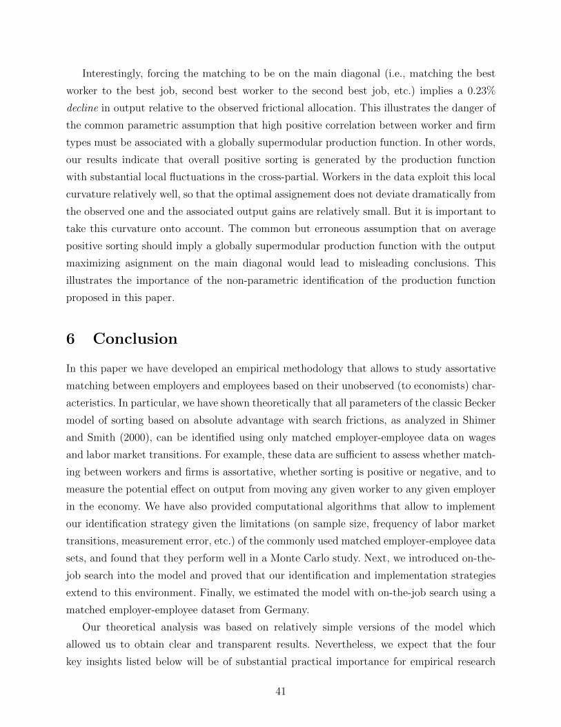
Interestingly, forcing the matching to be on the main diagonal (i.e., matching the best
worker to the best job, second best worker to the second best job, etc.) implies a 0.23%
decline in output relative to the observed frictional allocation. This illustrates the danger of
the common parametric assumption that high positive correlation between worker and firm
types must be associated with a globally supermodular production function. In other words,
our results indicate that overall positive sorting is generated by the production function
with substantial local fluctuations in the cross-partial. Workers in the data exploit this local
curvature relatively well, so that the optimal assignement does not deviate dramatically from
the observed one and the associated output gains are relatively small. But it is important to
take this curvature onto account. The common but erroneous assumption that on average
positive sorting should imply a globally supermodular production function with the output
maximizing asignment on the main diagonal would lead to misleading conclusions. This
illustrates the importance of the non-parametric identification of the production function
proposed in this paper.
6 Conclusion
In this paper we have developed an empirical methodology that allows to study assortative
matching between employers and employees based on their unobserved (to economists) char-
acteristics. In particular, we have shown theoretically that all parameters of the classic Becker
model of sorting based on absolute advantage with search frictions, as analyzed in Shimer
and Smith (2000), can be identified using only matched employer-employee data on wages
and labor market transitions. For example, these data are sufficient to assess whether match-
ing between workers and firms is assortative, whether sorting is positive or negative, and to
measure the potential effect on output from moving any given worker to any given employer
in the economy. We have also provided computational algorithms that allow to implement
our identification strategy given the limitations (on sample size, frequency of labor market
transitions, measurement error, etc.) of the commonly used matched employer-employee data
sets, and found that they perform well in a Monte Carlo study. Next, we introduced on-the-
job search into the model and proved that our identification and implementation strategies
extend to this environment. Finally, we estimated the model with on-the-job search using a
matched employer-employee dataset from Germany.
Our theoretical analysis was based on relatively simple versions of the model which
allowed us to obtain clear and transparent results. Nevertheless, we expect that the four
key insights listed below will be of substantial practical importance for empirical research
41

going forward. Each individual insight may or may not apply to every empirically relevant
model. But we do expect the combinations of these insights to be at the foundation of a
non-parametric identification and estimation strategy for the models in this class. These
insights are:
i) Within- and between-firm wage comparisons contain an extraordinary amount of in-
formation that can be exploited to identify relative worker productivities. Advances
in algorithm research allow a number of approaches to extract this information. We
exploit the one (rank aggregation) that applies to the models we consider. Other mod-
els may call for other methods, but they are readily available. We do not expect the
ranking of workers based on, say, lowest or highest wages to achieve similar precision.
ii) Firms can be ranked based on the value of the vacancy. This clearly will not be true in
every model, but we do expect this to be true in most empirically relevant models. One
piece of evidence for this is the empirical results in this paper. We very strongly reject
the hypothesis that the value of the vacancy is constant (e.g., zero). Our measurement
strategy is not biased towards finding this answer.
iii) Wage or surplus equations can be inverted for output. Not every model will permit such
an inversion, but many will. Once we know how to measure the value of unemployment
and the value of the vacancy (even if it is zero), non-parametric identification of the
production function immediately follows. We expect this to form the basis of any
attempt at non-parametric identification of the production function.
iv) The crucial element of our proposed implementation strategy that leads to very precise
estimates is binning of workers and firms. Given the limited time dimension of any
possible data, exploiting the cross-sectional variation will likely be the cornerstone of
any future attempt at non-parametric estimation.
There are numerous important positive and normative questions that can be answered
once the nonparametric identification of this class of models is established, in particular
of the production function and of the rankings of workers and firms. For example, as we
have shown, without any additional assumptions we can compute the optimal assignment
of workers to jobs on the set where match productivity can be measured. A comparison
between the optimal assignment and the observed one reveals the extent of the output loss
due to search frictions. A similar approach can be used to separately measure the extent of
changes in technology and sorting frictions over time (e.g, to understand the reasons for the
substantial rise in the college premium in the US in the 1980s) and across, say, countries. The
42
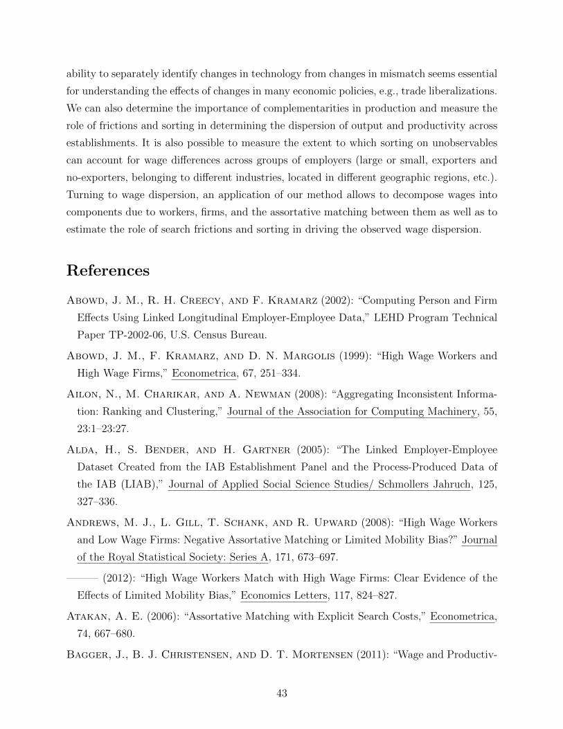
ability to separately identify changes in technology from changes in mismatch seems essential
for understanding the effects of changes in many economic policies, e.g., trade liberalizations.
We can also determine the importance of complementarities in production and measure the
role of frictions and sorting in determining the dispersion of output and productivity across
establishments. It is also possible to measure the extent to which sorting on unobservables
can account for wage differences across groups of employers (large or small, exporters and
no-exporters, belonging to different industries, located in different geographic regions, etc.).
Turning to wage dispersion, an application of our method allows to decompose wages into
components due to workers, firms, and the assortative matching between them as well as to
estimate the role of search frictions and sorting in driving the observed wage dispersion.
References
Abowd, J. M., R. H. Creecy, and F. Kramarz (2002): “Computing Person and Firm
Effects Using Linked Longitudinal Employer-Employee Data,” LEHD Program Technical
Paper TP-2002-06, U.S. Census Bureau.
Abowd, J. M., F. Kramarz, and D. N. Margolis (1999): “High Wage Workers and
High Wage Firms,” Econometrica, 67, 251–334.
Ailon, N., M. Charikar, and A. Newman (2008): “Aggregating Inconsistent Informa-
tion: Ranking and Clustering,” Journal of the Association for Computing Machinery, 55,
23:1–23:27.
Alda, H., S. Bender, and H. Gartner (2005): “The Linked Employer-Employee
Dataset Created from the IAB Establishment Panel and the Process-Produced Data of
the IAB (LIAB),” Journal of Applied Social Science Studies/ Schmollers Jahruch, 125,
327–336.
Andrews, M. J., L. Gill, T. Schank, and R. Upward (2008): “High Wage Workers
and Low Wage Firms: Negative Assortative Matching or Limited Mobility Bias?” Journal
of the Royal Statistical Society: Series A, 171, 673–697.
——— (2012): “High Wage Workers Match with High Wage Firms: Clear Evidence of the
Effects of Limited Mobility Bias,” Economics Letters, 117, 824–827.
Atakan, A. E. (2006): “Assortative Matching with Explicit Search Costs,” Econometrica,
74, 667–680.
Bagger, J., B. J. Christensen, and D. T. Mortensen (2011): “Wage and Productiv-
43

ity Dispersion: The Roles of Rent Sharing, Labor Quality and Capital Intensity,” mimeo.
Bagger, J. and R. Lentz (2014): “An Empirical Model of Wage Dispersion with Sorting,”
NBER Working Paper No. 20031.
Bartholdi, J., C. A. Tovey, and M. A. Trick (1989): “Voting Schemes for Which It
Can Be Difficult to Tell Who Won the Election,” Social Choice and Welfare, 6, 157–165,
10.1007/BF00303169.
Bartolucci, C. and F. Devicienti (2013): “Better Workers Move to Better Firms: A
Simple Test to Identify Sorting,” mimeo, Collegio Carlo Alberto.
Becker, G. (1973): “A Theory of Marriage: Part I,” Journal of Political Economy, 81,
813–846.
Bonhomme, S., T. Lamadon, and E. Manresa (2015): “A Distributional Framework
for Matched Employer Employee Data,” mimeo.
Burkard, R., M. DellAmico, and S. Martello (2009): Assignement Problems, SIAM.
Cahuc, P., F. Postel-Vinay, and J.-M. Robin (2006): “Wage Bargaining with On-
the-Job Search: Theory and Evidence,” Econometrica, 74, 323–364.
Card, D., J. Heining, and P. Kline (2013): “Workplace Heterogeneity and the Rise of
West German Wage Inequality,” The Quarterly Journal of Economics, 128, 967–1015.
Chade, H. (2001): “Two-Sided Search and Perfect Segregation with Fixed Search Costs,”
Mathematical Social Sciences, 42, 31–51.
Condorcet, J. (1785): “Essai sur l′application de l′analyse a la Probabilite des Decisions
Rendues a la pluralite des voix,” in American Mathematical Society Bookstore.
de Borda, J. C. (1781): Memoire sur les Elections au Scrutin, Paris: Histoire de l’Academie
Royale des Sciences.
Drissi-Bakhkhat, M. and M. Truchon (2004): “Maximum Likelihood Approach to
Vote Aggregation with Variable Probabilities,” Social Choice and Welfare, 23, 161–185.
Dustman, C., J. Ludsteck, and U. Schonberg (2009): “Revisiting the German Wage
Structure,” Quarterly Journal of Economics, 124, 363–376.
Eeckhout, J. and P. Kircher (2010): “Sorting and Decentralized Price Competition,”
Econometrica, 78, 539–574.
——— (2011): “Identifying Sorting – In Theory,” The Review of Economic Studies, 78,
872–906.
44
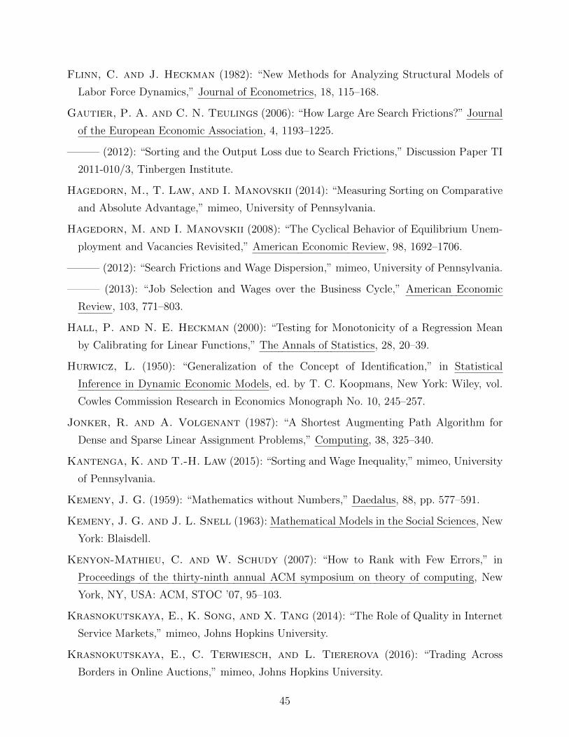
Flinn, C. and J. Heckman (1982): “New Methods for Analyzing Structural Models of
Labor Force Dynamics,” Journal of Econometrics, 18, 115–168.
Gautier, P. A. and C. N. Teulings (2006): “How Large Are Search Frictions?” Journal
of the European Economic Association, 4, 1193–1225.
——— (2012): “Sorting and the Output Loss due to Search Frictions,” Discussion Paper TI
2011-010/3, Tinbergen Institute.
Hagedorn, M., T. Law, and I. Manovskii (2014): “Measuring Sorting on Comparative
and Absolute Advantage,” mimeo, University of Pennsylvania.
Hagedorn, M. and I. Manovskii (2008): “The Cyclical Behavior of Equilibrium Unem-
ployment and Vacancies Revisited,” American Economic Review, 98, 1692–1706.
——— (2012): “Search Frictions and Wage Dispersion,” mimeo, University of Pennsylvania.
——— (2013): “Job Selection and Wages over the Business Cycle,” American Economic
Review, 103, 771–803.
Hall, P. and N. E. Heckman (2000): “Testing for Monotonicity of a Regression Mean
by Calibrating for Linear Functions,” The Annals of Statistics, 28, 20–39.
Hurwicz, L. (1950): “Generalization of the Concept of Identification,” in Statistical
Inference in Dynamic Economic Models, ed. by T. C. Koopmans, New York: Wiley, vol.
Cowles Commission Research in Economics Monograph No. 10, 245–257.
Jonker, R. and A. Volgenant (1987): “A Shortest Augmenting Path Algorithm for
Dense and Sparse Linear Assignment Problems,” Computing, 38, 325–340.
Kantenga, K. and T.-H. Law (2015): “Sorting and Wage Inequality,” mimeo, University
of Pennsylvania.
Kemeny, J. G. (1959): “Mathematics without Numbers,” Daedalus, 88, pp. 577–591.
Kemeny, J. G. and J. L. Snell (1963): Mathematical Models in the Social Sciences, New
York: Blaisdell.
Kenyon-Mathieu, C. and W. Schudy (2007): “How to Rank with Few Errors,” in
Proceedings of the thirty-ninth annual ACM symposium on theory of computing, New
York, NY, USA: ACM, STOC ’07, 95–103.
Krasnokutskaya, E., K. Song, and X. Tang (2014): “The Role of Quality in Internet
Service Markets,” mimeo, Johns Hopkins University.
Krasnokutskaya, E., C. Terwiesch, and L. Tiererova (2016): “Trading Across
Borders in Online Auctions,” mimeo, Johns Hopkins University.
45
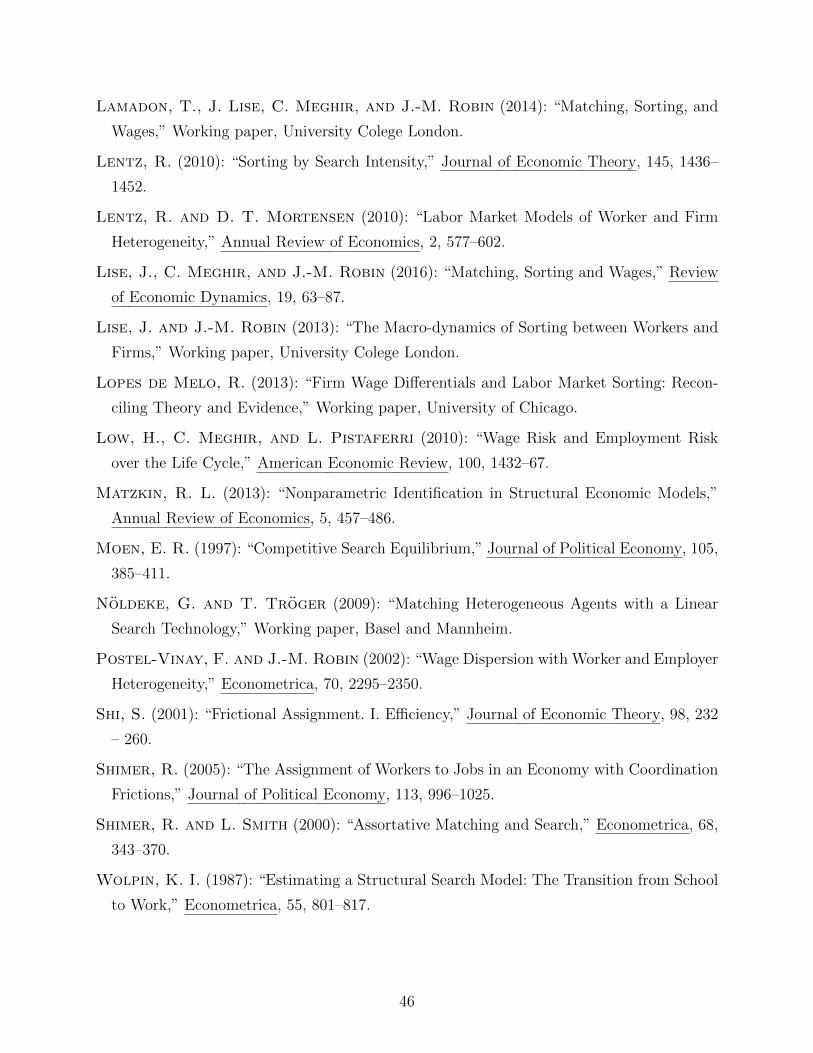
Lamadon, T., J. Lise, C. Meghir, and J.-M. Robin (2014): “Matching, Sorting, and
Wages,” Working paper, University Colege London.
Lentz, R. (2010): “Sorting by Search Intensity,” Journal of Economic Theory, 145, 1436–
1452.
Lentz, R. and D. T. Mortensen (2010): “Labor Market Models of Worker and Firm
Heterogeneity,” Annual Review of Economics, 2, 577–602.
Lise, J., C. Meghir, and J.-M. Robin (2016): “Matching, Sorting and Wages,” Review
of Economic Dynamics, 19, 63–87.
Lise, J. and J.-M. Robin (2013): “The Macro-dynamics of Sorting between Workers and
Firms,” Working paper, University Colege London.
Lopes de Melo, R. (2013): “Firm Wage Differentials and Labor Market Sorting: Recon-
ciling Theory and Evidence,” Working paper, University of Chicago.
Low, H., C. Meghir, and L. Pistaferri (2010): “Wage Risk and Employment Risk
over the Life Cycle,” American Economic Review, 100, 1432–67.
Matzkin, R. L. (2013): “Nonparametric Identification in Structural Economic Models,”
Annual Review of Economics, 5, 457–486.
Moen, E. R. (1997): “Competitive Search Equilibrium,” Journal of Political Economy, 105,
385–411.
Noldeke, G. and T. Troger (2009): “Matching Heterogeneous Agents with a Linear
Search Technology,” Working paper, Basel and Mannheim.
Postel-Vinay, F. and J.-M. Robin (2002): “Wage Dispersion with Worker and Employer
Heterogeneity,” Econometrica, 70, 2295–2350.
Shi, S. (2001): “Frictional Assignment. I. Efficiency,” Journal of Economic Theory, 98, 232
– 260.
Shimer, R. (2005): “The Assignment of Workers to Jobs in an Economy with Coordination
Frictions,” Journal of Political Economy, 113, 996–1025.
Shimer, R. and L. Smith (2000): “Assortative Matching and Search,” Econometrica, 68,
343–370.
Wolpin, K. I. (1987): “Estimating a Structural Search Model: The Transition from School
to Work,” Econometrica, 55, 801–817.
46
APPENDICES FOR ONLINE PUBLICATION
I Proofs and Derivations
I.1 Derivation of value functions
We derive workers’ value functions only since the functions for firms follow by symmetry.
An unemployed worker becomes employed only if he meets a firm in his acceptance
set, and does not experience immediate match destruction. Otherwise, the worker remains
unemployed in the next period.
Vu(x) = β(1− δ)Mu
∫Bw(x)
dv(y)
VVe(x, y) dy
︸ ︷︷ ︸successful matching
+ βδVu(x)︸ ︷︷ ︸destruction
+ β(1− δ)(1−Mu)Vu(x)︸ ︷︷ ︸no meeting
+ β(1− δ)MuVu(x)
∫Bw(x)
dv(y)
Vdy
︸ ︷︷ ︸meet unacceptable firm
.
To express the continuation value from successful matching in terms of surplus, subtract
Vu(x) from the first integrand and add it back to rebalance the equation. Then, use (1) to
obtain
Vu(x) = βα(1− δ)Mu
∫Bw(x)
dv(y)
VS(x, y) dy
+ βδVu(x) + β(1− δ)(1−Mu)Vu(x)
+ β(1− δ)MuVu(x)
∫Bw(x)
dv(y)
Vdy +
∫Bw(x)
dv(y)
Vdy
,where terms cancel to give (3).
An employed worker receives w(x, y), and remains employed next period with probability
(1− δ) or becomes unemployed with complementary probability. Minor rearranging and (1)
47
yield (5):
Ve(x, y) = w(x, y) + βδVu(x) + β(1− δ)Ve(x, y)
= w(x, y) + βδVu(x) + βα(1− δ)S(x, y) + β(1− δ)Vu(x)
= w(x, y) + βVu(x) + βα(1− δ)S(x, y).
I.2 Proofs of Results in Section 3.1
Proof of Result 1(i). Adding (5) and (6) yields:
Ve(x, y) + Vp(x, y) = f(x, y) + βVv(y) + βVu(x) + β(1− δ)S(x, y),
and, equivalently,
Ve(x, y)− Vu(x) + Vp(x, y)− Vv(y) = f(x, y) + (β − 1)Vv(y) + (β − 1)Vu(x)
+ β(1− δ)S(x, y),
so that, using (1), gives
S(x, y)(1− β(1− δ)) = f(x, y) + (β − 1)Vv(y) + (β − 1)Vu(x),
and thus surplus equals
S(x, y) =f(x, y) + (β − 1)Vv(y) + (β − 1)Vu(x)
1− β(1− δ). (A1)
Using (5) again, gives us wages32
w(x, y) = S(x, y)α(1− β(1− δ)) + (1− β)Vu(x)
= αf(x, y) + α(β − 1)Vv(y) + (1− α)(1− β)Vu(x). (A2)
32Wages can also be derived using (6):
w(x, y) = f(x, y)− S(x, y)(1− α)(1− β(1− δ)) + (β − 1)Vv(y)
= f(x, y)− (1− α)f(x, y)− (1− α)(β − 1)Vu(x) + α(β − 1)Vv(y)
= αf(x, y) + (1− α)(1− β)Vu(x) + α(β − 1)Vv(y).
48

We now establish that Vu(x) is increasing in x. From (3),
Vu(x)(1− β) = βα(1− δ)Mu
∫Bw(x)
dv(y)
VS(x, y) dy,
so that
∂Vu(x)
∂x(1− β) = βα(1− δ)Mu
∫Bw(x)
dv(y)
V
∂S(x, y)
∂xdy,
keeping in mind that either S(x, y) = 0 at the interior boundaries of the matching set or
the non-interior boundaries do not change with x. More precisely, consider for simplicity
Bw(x) = [ϕ(x), ϕ(x)]. If ϕ(x) 6= 0, then S(x, ϕ(x)) = 0. If ϕ(x) = 0, then∂ϕ(x)
∂x= 0.
Analogously, If ϕ(x) 6= 1, then S(x, ϕ(x)) = 0. If ϕ(x) = 1, then ∂ϕ(x)∂x
= 0.
As a result, we have, using (A1), that
∂Vu(x)
∂x(1− β) =
βα(1− δ)Mu
1− β(1− δ)
∫Bw(x)
dv(y)
V
∂f(x, y) + (β − 1)Vu(x)
∂xdy.
Solving for ∂Vu(x)∂x
yields
∂Vu(x)
∂x
1− β +(1− β)βα(1− δ)Mu
1− β(1− δ)
∫Bw(x)
dv(y)
Vdy
=
βα(1− δ)Mu
1− β(1− δ)
∫Bw(x)
dv(y)
V
∂f(x, y)
∂xdy
and thus ∂Vu(x)∂x
> 0 since ∂f(x,y)∂x
> 0.
To show that w(x, y) is increasing in x, we differentiate (A2):
∂w(x, y)
∂x= α
∂f(x, y)
∂x+ (1− α)(1− β)
∂Vu(x)
∂x,
which is positive because ∂f(x,y)∂x
> 0 and ∂Vu(x)∂x
> 0.
Finally, we show that Ve(x, y) is increasing in x as well. We have
Ve(x, y) = w(x, y) + βδVu(x) + β(1− δ)Ve(x, y),
49

and thus that
Ve(x, y)(1− β(1− δ)) = w(x, y) + βδVu(x),
which is increasing in x since ∂w(x,y)∂x
> 0 and ∂Vu(x)∂x
> 0.
Proof of Result 1(ii). Let ymin(x) be a firm type such that worker x is indifferent between
matching with this firm and staying unemployed,
Ve(x, ymin(x)) = Vu(x).
ymin(x) is the firm that pays the reservation wage to a worker of type x. Then (5) can be
written as
Ve(x, ymin(x)) = w(x, ymin(x)) + βVu(x),
so that
w(x, ymin(x)) = Ve(x, ymin(x))− βVu(x) = (1− β)Vu(x).
which from Result 1 (i) is increasing in x.
Proof of Result 1(iii). The maximum wage is given by w(x, ymax(x)). Taking derivatives
with respect to x yields
∂w(x, ymax(x))
∂x= wx(x, y
max(x)) + wy(x, ymax(x))ymaxx (x) = wx(x, y
max(x)) > 0.
Proof of Result 1(iv). Assume that the matching sets are unions of intervals. For the ease
of exposition we assume that there is just one interval:
Bw(x) = [ϕ(x), ϕ(x)].
First rewrite the adjusted average wage as
wav(x) = w(x, ymin(x)) + Mu(1− δ)∫
Bw(x)
dv(y)
V
[w(x, y)− w(x, ymin(x))
]dy.
50

Take derivatives with respect to x:
∂wav(x)
∂x=
∂w(x, ymin(x))
∂x+ Mu(1− δ)
∫Bw(x)
∂w(x, y)− w(x, ymin(x))
∂x
dv(y)
Vdy
+ Mu(1− δ)ϕ′(x)dv(ϕ(x))
V
[w(x, ϕ(x))− w(x, ymin(x))
]− Mu(1− δ)ϕ′(x)
dv(ϕ(x))
V
[w(x, ϕ(x))− w(x, ymin(x))
].
The last two terms are zero since either w(x, ϕ(x)) = w(x, ymin(x)) or ϕ′(x) = 0 and either
w(x, ϕ(x)) = w(x, ymin(x)) or ϕ′(x) = 0. Now simply rewrite
∂wav(x)
∂x=
∂w(x, ymin(x))
∂x
1−Mu + δMu + Mu(1− δ)∫
Bw(x)
dv(y)
Vdy
+ Mu(1− δ)
∫Bw(x)
∂w(x, y)
∂x
dv(y)
Vdy
to see that ∂wav(x)∂x
> 0.
I.3 Proofs of Results in Section 3.2
Proof of Result 2. For the value of a vacancy we have that
Vv(y)(1− β) = β(1− α)(1− δ)Mv
∫Bf (y)
du(x)
US(x, y) dx,
so that (using again as in the Proof of Result 1(i) that the terms involving the derivatives
of the boundaries are zero)
∂Vv(y)
∂y(1− β) = β(1− α)(1− δ)Mv
∫Bf (y)
du(x)U
∂f(x,y)+(β−1)Vv(y)∂y
1−β(1−δ) dx,
51

and thus that
∂Vv(y)
∂y(1− β +
(1− β)β(1− α)(1− δ)Mv
1− β(1− δ)
∫Bf (y)
du(x)
Udx)
= β(1− α)(1− δ)Mv
∫Bf (y)
du(x)
U
∂f(x,y)∂y
1− β(1− δ)dx > 0,
so that ∂Vv(y)∂y
> 0 since the coefficient multiplying it is positive. Finally we show that the
value of a filled job for a firm is increasing in y. We have that
Vp(x, y) = f(x, y)− w(x, y) + βVv(y) + β(1− α)(1− δ)S(x, y)
= f(x, y)(1− α)− (1− α)(1− β)Vu(x) + α(1− β)Vv(y) + βVv(y)
+ β(1− δ)(Vp(x, y)− Vv(y)),
so that
Vp(x, y)(1− β(1− δ)) = f(x, y)(1− α)− (1− α)(1− β)Vu(x) + Vv(y)(βδ + α(1− β)).
and
∂Vp(x, y)
∂y(1− β(1− δ)) =
∂f(x, y)
∂y(1− α) +
∂Vv(y)
∂y(βδ + α(1− β)) > 0.
Proof of Result 4. The main part of the proof is in the main text. Here we only show that
we can use Ω to rank firms even if some or all workers match with all firm types or if some
or all firms match with all worker types. In particular, we show that it does not matter that
if a worker of type x is accepted by all firms, the lowest wage w(x, ymin(x)) is not equal to
the reservation wage and thus not equal to the return of being unemployed.
The derivative of Ω with respect to y equals
∂Ω(y)
∂y= (1− δ)Mv
∫Bf (y)
du(x)
U
∂w(x, y)
∂ydx
+ (1− δ)Mv
(w(ϕ(y), y)− w(ϕ(y), ymin(ϕ(y))))
du(ϕ(y))
U
∂ϕ(y)
∂y
− (1− δ)Mv
(w(ϕ(y), y)− w(ϕ(y), ymin(ϕ(y))))
du(ϕ(y))
U
∂ϕ(y)
∂y
52
where for simplicity Bf (y) = [ϕ(y), ϕ(y)]. The terms (w(ϕ(y), y)−w(ϕ(y), ymin(ϕ(y))))∂ϕ(y)∂y
and (w(ϕ(y), y)− w(ϕ(y), ymin(ϕ(y))))∂ϕ(y)
∂yare both zero, because one of the two factors is
zero.
Without loss of generality consider the first term with ϕ(y). The argument for the second
term with ϕ(y) is identical. If the matching set is interior, that is ϕ(y) ∈ (0, 1), the lowest
wage of worker type ϕ(y), w(ϕ(y), ymin(ϕ(y))), is equal to the reservation wage and also
equal to w(ϕ(y), y). If the matching is not interior, that is ϕ(y) ∈ 0, 1, ∂ϕ(y)∂y
= 0.
Thus, independent of whether the matching set is interior or not, the term is zero and
the derivative of Ω with respect to y equals
∂Ω(y)
∂y= (1− δ)Mv
∫Bf (y)
du(x)
U
∂w(x, y)
∂ydx.
By the same logic, it holds that
∂∫
Bf (y)
du(x)U
(Ve(x, y)− Vu(x)) dx
∂y=
∫Bf (y)
du(x)
U
∂Ve(x, y)
∂ydx,
which is proportional to ∂Ω(y)∂y
since ∂Ve(x,y)∂y
(1− β(1− δ)) = ∂w(x,y)∂y
. As a result, the statistic
Ω(y) is increasing in y independent of the properties of the matching set.
I.4 Measuring α in the data
In the model of Shimer and Smith (2000), the value of α is fixed at 12. More generally, one
may consider leaving the value of α unrestricted in the (0, 1) interval and recovering it from
the data. Note that α governs the responsiveness of wages to changes in match surplus (if
α→ 0, workers receive b regardless of the movements in the match surplus, while if α→ 1,
workers’ wages fully co-move with surplus). While this provides a natural source of variation
for the identification of this parameter, the fluctuations of surplus are absent form the simple
baseline version of the model considered in the main text. In this appendix we extend the
model to incorporate two sources of fluctuation in match surplus, an idiosyncratic and an
aggregate productivity shock and show how each of these stochastic components allows to
identify the bargaining powers.33
33Eeckhout and Kircher (2011) have argued that the bargaining power can also be identified in the baselinedeterministic version of the model. Unfortunately, their proof appears to contain a mistake (Eq. (28) in theirpaper does not follow from Eq. (26) since the term w∗x(x) is missing in Eq. (28)).
53
I.4.1 Measure α from fluctuation in firm output
To measure the bargaining power α in the data, we first consider an extended version of the
model with i.i.d. shocks to the firm’s technology, εj, which changes output from f(x, y) to
f(x, y)+εj for all worker types x employed at firm j of type y. In response to such a shock to
the firm’s technology, Nash bargaining with worker bargaining power α implies that profits
increase by (1 − α) and wages increase by α. To measure α using this experiment we can
use any data where the response of wages is observable. This approach for identifying the
bargaining powers was pursued in a number of papers in the literature reviewed in Hagedorn
and Manovskii (2008).
Adding these shocks to our model is simple and does not change any of our other re-
sults and conclusions as we verified in simulated data. The reason is that these shocks are
unanticipated and their impact is only to make statistics slightly noisier in the same way
as measurement error does (and we have established in the main text that adding a large
amount of measurement error does not have a significant impact on our inference). The rank-
ing of workers within a firm is not affected at all since all wages within a firm are shifted by
the same amount, αεj, and thus the ranking of workers is preserved. The ranking of firms is
based on the statistic Ω which is proportional to the value of a vacancy. Since the technology
shocks are unanticipated this statistic is not affected either. Neither is the estimation of the
production function f . The only object that is affected is the estimation of the matching
set, as now workers may become acceptable only because of a large positive εj whereas they
were not acceptable in the absence of any shocks. This makes the model computationally
much more burdensome. Given that adding these idiosyncratic shocks to the model obviously
allows to identify α but has no material impact on any of our results, we adopted a simpler
model as a benchmark in the main text.
I.4.2 Using Business Cycles to Measure α
We now show how the bargaining power α can be measured in the data by considering
an extended version of the model with business cycles, i.e. exogenous changes in aggregate
productivity z. The output of a pair (x, y) is then zf(x, y). Consider two worker types x
and x′ (have to be different types), working at firm y when productivity is z and when it
is z. The wages of worker x in the two business cycle states are w(x, y, z) and w(x, y, z),
respectively. For worker x′ the corresponding wages are w(x′, y, z) and w(x′, y, z). These
wages are observed. The equation for wages with business cycles is straightforward and
follows the same arguments as the one without business cycles. For the value of a job it
54
holds with the obvious notation that
Ve(x, y, z) = w(x, y, z) + βE(Vu(x, z′) | z) + βα(1− δ)E(S(x, y, z′) | z),
and for the value of a filled vacancy that
Vp(x, y, z) = zf(x, y)− w(x, y, z) + βE(Vv(y, z′) | z) + β(1− α)(1− δ)E(S(x, y, z′) | z).
Adding up these two Bellman equations yields:
Ve(x, y, z) + Vp(x, y, z) = zf(x, y) + βE(Vv(y, z′) | z) + βE(Vu(x, z
′) | z)
+β(1− δ)E(S(x, y, z′) | z),
and equivalently
S(x, y, z) = Ve(x, y, z)− Vu(x, z) + Vp(x, y, z)− Vv(y, z)
= zf(x, y)− Vv(y, z)− Vu(x, z) + βE(Vv(y, z′) | z) + βE(Vu(x, z
′) | z)
+β(1− δ)E(S(x, y, z′) | z).
Motivated by the observation that productivity basically follows a random walk, we now
make the approximation that
E(S(x, y, z′) | z) = S(x, y, z) + expectational error,
so that the surplus equals
S(x, y, z)(1− β(1− δ)) = zf(x, y)− Vv(y, z)− Vu(x, z) + βE(Vv(y, z′) | z)
+βE(Vu(x, z′) | z).
Using the Bellman equation for Ve and the approximation we can solve for wages:
w(x, y, z) = αS(x, y, p)(1− β(1− δ)) + Ve(x, z)− βE(Vu(x, z′) | z).
Making the same approximation for Vu,
E(Vu(x, z′) | z) = Vu(x, z) + expectational error,
55
and using the equation for the surplus S, we obtain
w(x, y, z) = α(zf(x, y)− Vv(y, z)− (1− β)Vu(x, z) + βE(Vv(y, z′) | z))
+Vu(x, z)(1− β)
= αzf(x, y) + α(βE(Vv(y, z′) | z)− Vv(y, z)) + (1− α)(1− β)Vu(x, z).
The differences in wages for types x and x′ equals
w(x′, y, z)− w(x, y, z) = αz(f(x′, y)− f(x, y)) + (1− α)(1− β)(Vu(x′, z)− Vu(x, z)).
To figure out α we have to measure Vu(x, z) and Vu(x′, z) in the data. For this we use the
Bellman equation for Ve and the approximation for the expected surplus
Vu(x, z) = Ve(x, y(x, z), z)
= w(x, y(x, z), z) + βE(Vu(x, z′) | z) + βα(1− δ)E(S(x, y(x, z), z′) | z)
= w(x, y(x, z), z) + βVu(x, z) + βα(1− δ)S(x, y(x, z), z)
= w(x, y(x, z), z) + βVu(x, z),
so that
Vu(x, z)(1− β) = w(x, y(x, z), z),
i.e., we measure the value of employment at the lowest firm at productivity level z through
the lowest wage accepted by type x at level z. Using this expression for the reservation wage
in the wage equation to substitute for the value of unemployment, yields
w(x′, y, z)− w(x, y, z)
= αz(f(x′, y)− f(x, y)) + (1− α)(1− β)(Vu(x′, z)− Vu(x, z))
= αz(f(x′, y)− f(x, y)) + (1− α)(w(x′, y(x′, z), z)− w(x, y(x, z), z)).
For the empirical implementation define then dummies δx,y which is one if worker type x
works at firm type y and zero otherwise. We then regress
wt(x′)− wt(x) = zt(δx′,y − δx,y) + κ(w(x′, y(x′, z), z)− w(x, y(x, z), z)).
The estimated value of κ is then our estimate of 1− α so that α = (1− κ).
56

II Computation and Implementation
In this section we describe how we compute the model, construct and measure the variables
mentioned in the text. We first discretize the continuous type space for both workers and firms
with 50 evenly distributed grid points on the type space [0, 1]. To compute the model we use
an iterative procedure on the match density, dm(x, y) and the surplus, S(x, y). Let dm,k(x, y)
and Sk(x, y) be the values in the kth iteration. To initialize the iteration, we set, ∀(x, y),
the initial match distribution, dm,0(x, y) = 0.5, and the initial surplus, S0(x, y) = f(x, y).
We obtain a solution by alternatively updating exactly once on either the match density
(Eq. 8) or the flow equation for the surplus (which we get by summing Eq. 3 - 6). When
dm,k(x, y) < 10−6, we set dm,k(x, y) = 0. A solution is found if the maximum absolute
difference between iterations of both surplus and match density is less than 10−12.
If no solution admitting a pure acceptance strategy is found (due to discretization),
we solve for a mixed strategy; i.e., unemployed agents accept matches with a probability
(between 0 and 1) such that the surplus of the match is positive, but very close to zero.
Denote iteration k of the acceptance strategy of workers with Awk (x, y). Awk (x, y) is the
probability worker x accepts a job at firm y. We then update the acceptance strategy in the
following way.
Mixed strategy
if Sk(x, y) > 5× 10⁻⁷ and Awk (x, y) < 1
Awk+1(x, y) = Awk (x, y) + 0.001 · rand() · (1− Awk (x, y))
elseif Sk(x, y) < 5× 10⁻⁷ and Awk (x, y) > 0
Awk+1(x, y) = Awk (x, y)− 0.001 · rand() · (1− Awk (x, y)),
end
where rand() is a pseudo-random value drawn from the standard uniform distribution on
the open interval (0, 1). A mixed solution is found if the maximum absolute change between
iterations of both the surplus and the match density are less than 2.5 × 10⁻⁶. We find a
mixed strategy solution in all parameterizations that we use.
With the computed solution, we simulate 600 workers and 600 jobs for each grid point
giving 60000 agents (30000 workers and 30000 jobs) over a period of 240 months with an
initial burn-in of 100 months. This corresponds to 20 years of monthly data.
Where order is meaningful (e.g. ranks, types or bins), higher numbers correspond to
higher productivity; e.g., a worker with rank 10 is better than a worker with rank 2, a firm
in bin 7 is better than a firm in bin 3.
Here, we define quantities that we will use to sketch the procedures we use.
57
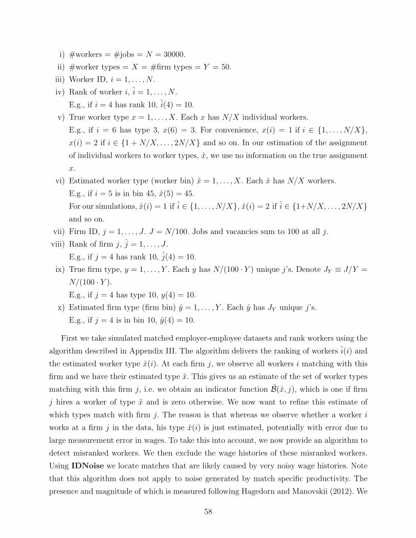
i) #workers = #jobs = N = 30000.
ii) #worker types = X = #firm types = Y = 50.
iii) Worker ID, i = 1, . . . , N .
iv) Rank of worker i, i = 1, . . . , N .
E.g., if i = 4 has rank 10, i(4) = 10.
v) True worker type x = 1, . . . , X. Each x has N/X individual workers.
E.g., if i = 6 has type 3, x(6) = 3. For convenience, x(i) = 1 if i ∈ 1, . . . , N/X,x(i) = 2 if i ∈ 1 + N/X, . . . , 2N/X and so on. In our estimation of the assignment
of individual workers to worker types, x, we use no information on the true assignment
x.
vi) Estimated worker type (worker bin) x = 1, . . . , X. Each x has N/X workers.
E.g., if i = 5 is in bin 45, x(5) = 45.
For our simulations, x(i) = 1 if i ∈ 1, . . . , N/X, x(i) = 2 if i ∈ 1+N/X, . . . , 2N/Xand so on.
vii) Firm ID, j = 1, . . . , J . J = N/100. Jobs and vacancies sum to 100 at all j.
viii) Rank of firm j, j = 1, . . . , J .
E.g., if j = 4 has rank 10, j(4) = 10.
ix) True firm type, y = 1, . . . , Y . Each y has N/(100 · Y ) unique j’s. Denote JY ≡ J/Y =
N/(100 · Y ).
E.g., if j = 4 has type 10, y(4) = 10.
x) Estimated firm type (firm bin) y = 1, . . . , Y . Each y has JY unique j’s.
E.g., if j = 4 is in bin 10, y(4) = 10.
First we take simulated matched employer-employee datasets and rank workers using the
algorithm described in Appendix III. The algorithm delivers the ranking of workers i(i) and
the estimated worker type x(i). At each firm j, we observe all workers i matching with this
firm and we have their estimated type x. This gives us an estimate of the set of worker types
matching with this firm j, i.e. we obtain an indicator function B(x, j), which is one if firm
j hires a worker of type x and is zero otherwise. We now want to refine this estimate of
which types match with firm j. The reason is that whereas we observe whether a worker i
works at a firm j in the data, his type x(i) is just estimated, potentially with error due to
large measurement error in wages. To take this into account, we now provide an algorithm to
detect misranked workers. We then exclude the wage histories of these misranked workers.
Using IDNoise we locate matches that are likely caused by very noisy wage histories. Note
that this algorithm does not apply to noise generated by match specific productivity. The
presence and magnitude of which is measured following Hagedorn and Manovskii (2012). We
58
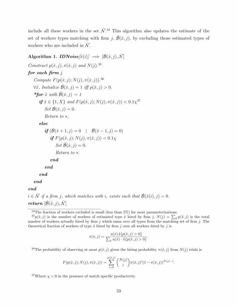
include all these workers in the set N .34 This algorithm also updates the estimate of the
set of workers types matching with firm j, B(x, j), by excluding those estimated types of
workers who are included in N .
Algorithm 1. IDNoise[x(i)] =⇒ [B(x, j), N ]
Construct p(x, j), π(x, j) and N(j).35
for each firm j
Compute F (p(x, j);N(j), π(x, j)).36
∀x, Initialize B(x, j) = 1 iff p(x, j) > 0.
*for x with B(x, j) = 1
if x ∈ 1, X and F (p(x, j);N(j), π(x, j)) < 0.1χ37
Set B(x, j) = 0.
Return to ∗.else
if (B(x+ 1, j) = 0 | B(x− 1, j) = 0)
if F (p(x, j);N(j), π(x, j)) < 0.1χ
Set B(x, j) = 0.
Return to ∗.end
end
end
end
end
i ∈ N if a firm j, which matches with i, exists such that B(x(i), j) = 0.
return [B(x, j), N ]
34The fraction of workers excluded is small (less than 5%) for most parameterizations.35p(x, j) is the number of workers of estimated type x hired by firm j. N(j) =
∑x p(x, j) is the total
number of workers actually hired by firm j which sums over all types from the matching set of firm j. Thetheoretical fraction of workers of type x hired by firm j over all workers hired by j is
π(x, j) =u(x)1p(x, j) > 0∑x u(x) · 1p(x, j) > 0
.
36The probability of observing at most p(x, j) given the hiring probability π(x, j) from N(j) trials is
F (p(x, j);N(j), π(x, j)) =
p(x,j)∑i=0
(N(j)
i
)π(x, j)i(1− π(x, j))N(j)−i.
37Where χ = 0 in the presence of match specific productivity.
59

The next crucial statistic to estimate is reservation wages for each worker wres(i). To this
end, we implement ResWage.
Algorithm 2. ResWage[w(i, j), x(i), N ] =⇒ wres(i)
Consider wages histories of i /∈ N .
for x
Construct J(x) = j s.t. j hires any i ∈ x.foreach j ∈ J(x), compute w(x, j) = average wage paid by j to workers i ∈ x.
wres(x) = lowest average of w(x, j) possible from pooling JY firms in J .38
end
return wres(i) = wres(x(i))
Then, for each firm j, compute the average wage premium as in (15). We next estimate
job filling rates q(j) using information from all workers (whether or not they belong to N )
over the acceptance set B of firm j, which includes all types x for which B(x, j) = 1. Our
estimate of q(j) is Mv
∑x∈B
u(x)u
. Multiplying the average wage premium and the acceptance
rate gives the statistic Ω which allows us to rank firms.
We now assign individual firms to firm types y. Using our ranking of firms, we can assign
the first JY firms to firm bin 1, the next JY firms to firm bin 2, and so on. The assignment of
firms to types allows us to compute statistics for firm types only. For example, statistics for
all firms belonging to firm type y = 1 will be the firm size (measured by average employment)
weighted average of firms with j(j) ∈ 1..JY . This step only serves to aggregate information
across firms and yields smoother statistics and more precise estimates. We could have also
proceeded by assigning each individual firm to its own type, i.e. y(j) = j(j).
Taking present values of estimated minimum wages for each bin yields Vu(x). Compute
the average wages each bin x receives with all firms of bin y. This is wav(x, y). Compute
the corresponding value of employment, Ve(x, y) and Vv(y) from Ω(y). The estimate of the
production function f(x, y) follows.
Using unemployment rates at the x level and estimated firm size at the j level, we can
estimate frictional output with the estimated production function.
To measure output losses due to frictions we optimally assign a sub-sample (5000 workers
and 5000 jobs) from the pool of employed workers.39 The sub-sample reflects the estimated
type distributions of employed workers and producing firms. To evaluate the accuracy of
38For x > 1 , we additionally impose wres(x) > wres(x− 1) which is consistent with theory.39See Section 4.6 for references to the algorithms used.
60
our method, our estimated gains from eliminating search frictions is compared the same
procedure repeated using true model generated distributions and production functions.
III Rank aggregation
Our goal is to rank workers according to their productivity. We know that wages within a
firm are increasing in worker productivity x. Thus, in the absence of measurement error,
considering the workers within one specific firm gives us a correct ranking among these
workers. Repeating this ranking for every firm yields a globally consistent and, if workers
are sufficiently mobile between firms, a complete ranking of workers since worker rankings
are transitive across firms.
However, wage data might contain measurement error. Consequently, within one firm,
a less productive worker could be ranked above a truly more productive worker because
of measurement error. Furthermore, the ranking between these two workers may not be
transitive across firms where they happen to be co-workers. Thus, the rankings from all
firms are not consistent and thus do not yield an aggregate ranking. To solve this problem,
we build on the insights from social choice theory, which considers a equivalent problem in
the context of voting.
Imagine that voters were asked to rank candidates from the most to the least preferred
one. Voters will rank candidates according to their own preferences but when the need to
have a single ranking of candidates comes up, a disagreement is likely to arise. Unless every
voter ranks all candidates identically, there will not be an aggregate ranking that all voters
agree with completely. This requires then the specification of how to aggregate disagreements
between voters and a method how to find this aggregate ranking.
III.1 Kemeny-Young rank aggregation
Given many (perhaps) inconsistent rankings of candidates, how does one aggregate the ranks
to determine who the best candidate is? This problem is ancient, and first studied by de Borda
(1781) and Condorcet (1785). One natural starting point to use as a metric for evaluating the
posited aggregate ranking is the number of disagreements generated in the voter submitted
ranks as done in the Kemeny-Young formulation of this classic problem.40 The goal then
is to find an aggregate ranking which generates the minimum number of disagreements
with the data. Drissi-Bakhkhat and Truchon (2004) argue in a context of a social choice
40This is first described in Kemeny (1959) and Kemeny and Snell (1963)
61

model that the disagreements in the ranking of two alternatives should be weighted by the
probability that the voters compare them correctly. Similarly, in our labor market application
weighting means that the disagreements are weighted by the probabilities that a worker is
ranked higher than another worker (which are computed from wage data). Fortunately, the
computer science literature provides algorithms to handle these weighted ranking problems
as well since they can be cast as a special case of a weighted feedback arc set problem on
tournaments (see for example Ailon et al. (2008)).
For a candidate ranking Π, Π(i, j) = 1 if i is ranked higher than j and Π(i, j) = 0
otherwise. There are no ties. The objective is to find ranking Π which maximizes
∑i>j
c(i, j)Π(i, j) + c(j, i)Π(j, i), (A3)
where the weighting c(i, j) is the probability (computed from wage observations) that i
is ranked above j.
We now construct c(i, j). First, we use head-to-head wage information at all firms to
calculate the probability that worker i is ranked higher than worker j. Note, that we can
only use this ranking when we observe worker i and worker j at the same firm. We first
discuss the simple case where we only observe i and j at one firm.
Suppose we observe ni,k wage observations and nj,k from workers i and j respectively at
firm k.41 We know that observed wages follows:
wi,k,t = wi,k + εt
which contains noise ε with variance σ2. We can compute the average wages wi,k and wj,k,
which can be written as:
wi,k − wj,k =1
ni,k
ni,k∑t=1
wi,k,t −1
nj,k
nj,k∑t=1
wj,k,t
= wi,k − wj,k +1
ni,k
ni,k∑t=1
εi,k,t −1
nj,k
nj,k∑t=1
εj,k,t,
where all of the ε’s are independent.
We are interested in computing the probability that wi,k > wj,k given the observations
on wi,k and wj,k. A Bayesian approach seems a natural one to follow to accomplish this.
41ni,k periods (months, in our case) of observations need not be in one employment spell. Moreover, i andj do not need to be employed at the same time.
62

Suppose that we had a normal prior distribution over wages, that is we assume that:
wi,k ∼ N (µ0, τ20 ).
The posterior density over wi,k conditional on knowing σ2 (we explain below how to measure
it in the data) is given by:
p(wi,k|wi,k,1, · · · , wi,k,ni,k) = p(wi,k|wi,k) = N (µn, τ2n),
where
µn =
1τ20µ0 +
ni,kσ2 wi,k
1τ20
+ni,kσ2
and1
τ 2n
=1
τ 20
+ni,kσ2
.
If in the baseline case we assume an uninformative prior, that is, we take τ 20 → ∞, this
simplifies to:
µn = wi,k
and1
τ 2n
=ni,kσ2
.
Then the posterior densities for wi,k, wj,k given the data would just be given by:
p(wi,k|wi,k) = N(wi,k,
σ2
ni,k
),
p(wj,k|wj,k) = N(wj,k,
σ2
nj,k
).
Since these posteriors are independent normals, we know that the distribution over the
difference p(wi,k − wj,k|wi,k, wj,k) is simply:
p (wi,k − wj,k|wi,k, wj,k) = N(wi,k − wj,k,
σ2
ni,k+
σ2
nj,k
).
63
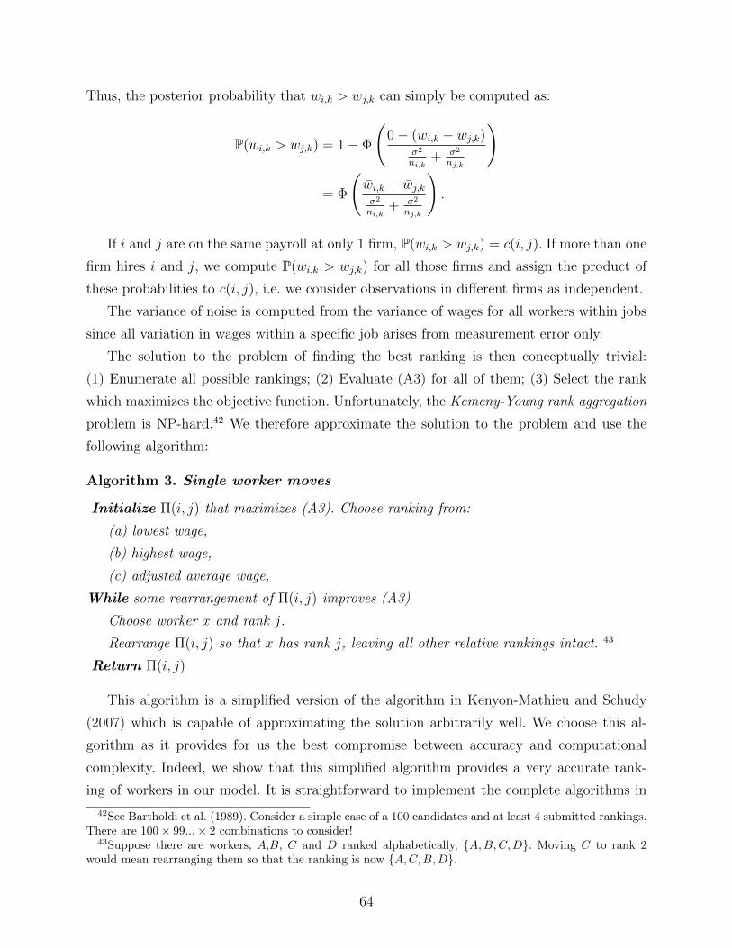
Thus, the posterior probability that wi,k > wj,k can simply be computed as:
P(wi,k > wj,k) = 1− Φ
(0− (wi,k − wj,k)
σ2
ni,k+ σ2
nj,k
)
= Φ
(wi,k − wj,kσ2
ni,k+ σ2
nj,k
).
If i and j are on the same payroll at only 1 firm, P(wi,k > wj,k) = c(i, j). If more than one
firm hires i and j, we compute P(wi,k > wj,k) for all those firms and assign the product of
these probabilities to c(i, j), i.e. we consider observations in different firms as independent.
The variance of noise is computed from the variance of wages for all workers within jobs
since all variation in wages within a specific job arises from measurement error only.
The solution to the problem of finding the best ranking is then conceptually trivial:
(1) Enumerate all possible rankings; (2) Evaluate (A3) for all of them; (3) Select the rank
which maximizes the objective function. Unfortunately, the Kemeny-Young rank aggregation
problem is NP-hard.42 We therefore approximate the solution to the problem and use the
following algorithm:
Algorithm 3. Single worker moves
Initialize Π(i, j) that maximizes (A3). Choose ranking from:
(a) lowest wage,
(b) highest wage,
(c) adjusted average wage,
While some rearrangement of Π(i, j) improves (A3)
Choose worker x and rank j.
Rearrange Π(i, j) so that x has rank j, leaving all other relative rankings intact. 43
Return Π(i, j)
This algorithm is a simplified version of the algorithm in Kenyon-Mathieu and Schudy
(2007) which is capable of approximating the solution arbitrarily well. We choose this al-
gorithm as it provides for us the best compromise between accuracy and computational
complexity. Indeed, we show that this simplified algorithm provides a very accurate rank-
ing of workers in our model. It is straightforward to implement the complete algorithms in
42See Bartholdi et al. (1989). Consider a simple case of a 100 candidates and at least 4 submitted rankings.There are 100× 99...× 2 combinations to consider!
43Suppose there are workers, A,B, C and D ranked alphabetically, A,B,C,D. Moving C to rank 2would mean rearranging them so that the ranking is now A,C,B,D.
64
Kenyon-Mathieu and Schudy (2007) if more precision is required for a particular application.
IV Model with On-the-job Search
We first describe the details of the model with on-the-job search used in the data analysis.
We then prove the results, mentioned in the main text, to obtain identification and we finally
evaluate its performance in Monte Carlo simulations.
IV.1 The Model
In this Section we describe the model which introduces on-the-job search into the environ-
ment of Shimer and Smith (2000) analyzed in the main text. The basic features of the two
models are the same and we describe here only the necessary modifications.
All workers and all unmatched firms engage in random search. The exogenous search
intensity of employed (relative to unemployed workers) is φ ∈ [0, 1]. The total search effort
is the weighted sum s = U + φE. A function m : [0, 1] × [0, 1] → [0,min(s, V )] takes
the total mass of searchers s and vacant firms V as its inputs and generates meetings. The
probabilities that an unemployed or an employed worker meets a potential employer are given
by Mu = m(s,V )s
, and Me = φm(s,V )s
, while the probability of a vacant firm meeting a potential
hire is Mv = m(s,V )V
. These probabilities are time-invariant in the steady-state equilibrium
we will consider. The probability to meet a firm y ∈ Y ⊂ [0, 1] equals Mu
∫Y dv(y)dy
Vfor
unemployed and Me
∫Y dv(y)dy
Vfor employed workers. For firms, these probabilities depend on
the employment status of the worker, since unemployed and employed workers not only search
with different intensities but also endogenously exhibit different distributions. Conditional
on meeting a worker, we therefore define the probabilities that the worker is unemployed or
employed by Cu = UU+φE
and Ce = φEU+φE
, respectively. The probability for a firm to meet an
unemployed worker x ∈ X ⊂ [0, 1] then equals MvCu
∫X du(x)dx
Uand the probability to meet
an employed worker x ∈ X ⊂ [0, 1] equals MvCe
∫X de(x)dx
E. Not all meetings necessarily result
in matches. Some meetings are between an unemployed worker and a vacant firm who are
unwilling to consummate a match and who prefer to continue the search process. Some other
meetings are between an employed worker and a vacant firm where the worker prefers to
stay with the current firm so that the meeting does not result in a new match.
An unemployed worker makes a take-it-or-leave-it offer to a firm and thus extracts the
full surplus. As in Postel-Vinay and Robin (2002) and Cahuc et al. (2006), when a worker
employed at some firm y meets a firm y which generates higher surplus, the two firms engage
65
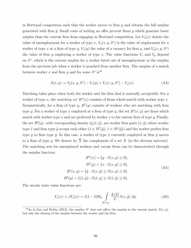
in Bertrand competition such that the worker moves to firm y and obtains the full surplus
generated with firm y. Small costs of writing an offer prevent firms y which generate lower
surplus than the current firm from engaging in Bertrand competition. Let Vu(x) denote the
value of unemployment for a worker of type x, Ve(x, y, So) is the value of employment for a
worker of type x at a firm of type y, Vv(y) the value of a vacancy for firm y, and Vp(x, y, So)
the value of firm y employing a worker of type x. The value functions Ve and Vp depend
on So, which is the current surplus for a worker hired out of unemployment or the surplus
from the previous job when a worker is poached from another firm. The surplus of a match
between worker x and firm y and for some So is44
S(x, y) := Vp(x, y, So)− Vv(y) + Ve(x, y, S
o)− Vu(x). (A4)
Matching takes place when both the worker and the firm find it mutually acceptable. For a
worker of type x, the matching set Bw(x) consists of firms which match with worker type x.
Symmetrically, for a firm of type y, Bf (y) consists of workers who are matching with firm
type y. For a worker of type x employed at a firm of type y, the set Be(x, y) are firms which
match with worker type x and are preferred by worker x to his current firm of type y. Finally,
the set Bp(y), with corresponding density dy(x, y), are worker firm pairs (x, y) where worker
type x and firm type y accept each other (x ∈ Bf (y), x ∈ Bu(y)) and the worker prefers firm
type y to firm type y. In this case, a worker of type x currently employed at firm y moves
to a firm of type y. We denote by X the complement of a set X (in the obvious universe).
The matching sets for unemployed workers and vacant firms can be characterized through
the surplus function:
Bw(x) = y : S(x, y) ≥ 0,
Bf (y) = x : S(x, y) ≥ 0,
Be(x, y) = y : S(x, y) ≥ S(x, y) ≥ 0,
Bp(y) = (x, y) : S(x, y) ≥ S(x, y) ≥ 0.
(A5)
The steady state value functions are:
Vu(x) = βVu(x) + β(1− δ)Mu
∫Bu(x)
dv(y)
VS(x, y) dy, (A6)
44As in Lise and Robin (2013), the surplus So does not affect the surplus in the current match, S(x, y),but only the sharing of the surplus between the worker and the firm.
66
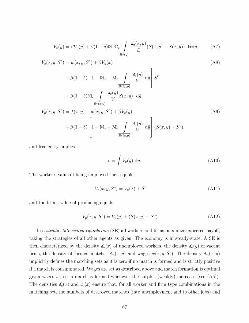
Vv(y) = βVv(y) + β(1− δ)MvCe
∫Bp(y)
dy(x, y)
E(S(x, y)− S(x, y)) dxdy, (A7)
Ve(x, y, So) = w(x, y, So) + βVu(x) (A8)
+ β(1− δ)
1−Me + Me
∫Be(x,y)
dv(y)
Vdy
S0
+ β(1− δ)Me
∫Be(x,y)
dv(y)
VS(x, y) dy,
Vp(x, y, So) = f(x, y)− w(x, y, So) + βVv(y) (A9)
+ β(1− δ)
1−Me + Me
∫Be(x,y)
dv(y)
Vdy
(S(x, y)− So),
and free entry implies
c =
∫Vv(y) dy. (A10)
The worker’s value of being employed then equals
Ve(x, y, So) = Vu(x) + So (A11)
and the firm’s value of producing equals
Vp(x, y, So) = Vv(y) + (S(x, y)− So). (A12)
In a steady state search equilibrium (SE) all workers and firms maximize expected payoff,
taking the strategies of all other agents as given. The economy is in steady-state. A SE is
then characterized by the density du(x) of unemployed workers, the density dv(y) of vacant
firms, the density of formed matches dm(x, y) and wages w(x, y, So). The density dm(x, y)
implicitly defines the matching sets as it is zero if no match is formed and is strictly positive
if a match is consummated. Wages are set as described above and match formation is optimal
given wages w, i.e. a match is formed whenever the surplus (weakly) increases (see (A5)).
The densities du(x) and dv(x) ensure that, for all worker and firm type combinations in the
matching set, the numbers of destroyed matches (into unemployment and to other jobs) and
67

created matches (hires from unemployment and from other jobs) are the same.
IV.2 Identification
IV.2.1 Some Useful results
Before we turn to the specific identification results, we derive results for the surplus and
wages. We first derive the Bellman equation of surplus:
S(x, y) = Vp(x, y, So)− Vv(y) + Ve(x, y, S
o)− Vu(x)
= f(x, y)− (1− β)(Vv(y) + Vu(x))
+ β(1− δ)
1−Me + Me
∫Be(x,y)
dv(y)
Vdy
S(x, y)
+ β(1− δ)Me
∫Be(x,y)
dv(y)
VS(x, y) dy,
= f(x, y)− (1− β)(Vv(y) + Vu(x)) + β(1− δ)S(x, y)
so that
S(x, y)[1− β(1− δ)] = f(x, y)− (1− β)(Vv(y) + Vu(x)). (A13)
We can also compute how the surplus changes with worker type x:
∂S(x, y)
∂x=
∂f(x,y)∂x− (1− β)∂Vu(x)
∂x
1− β(1− δ). (A14)
Similarly, the derivative with respect to y equals:
∂S(x, y)
∂y=
∂f(x,y)∂y− (1− β)∂Vv(y)
∂y
1− β(1− δ). (A15)
68

From the Bellman equation for an employed worker, we get that the wage equals
w(x, y, So) = So + (1− β)Vu(x) (A16)
− β(1− δ)
1−Me + Me
∫Be(x,y)
dv(y)
Vdy
S0
− β(1− δ)Me
∫Be(x,y)
dv(y)
VS(x, y) dy.
For a worker coming out of unemployment this equals
w(x, y, So) = S(x, y) + (1− β)Vu(x)− β(1− δ)S(x, y). (A17)
And thus using the surplus equation
w(x, y, So) = f(x, y)− (1− β)(Vv(y) + Vu(x)) + (1− β)Vu(x)
= f(x, y)− (1− β)Vv(y). (A18)
Finally, we can also show that workers can be ranked by their lowest as well as by their
highest wage. Let ymin(x) be a firm type such that worker x is indifferent between matching
with this firm and staying unemployed,
Ve(x, ymin(x)) = Vu(x).
ymin(x) is the firm that pays the lowest wage to a worker of type x hired from unemployment.
Of course, this equation can be satisfied for more than one firm. In this case simply pick the
lowest firm type. It then holds that (from the Bellman equation for Ve):
Ve(x, ymin(x)) = w(x, ymin(x)) + βVu(x)
+ β(1− δ)Me
∫Be(x,ymin(x))
dv(y)
VS(x, y) dy
and from the Bellman equation for Vu
Vu(x)(1− β) = β(1− δ)Mu
∫Bw(x)
dv(y)
VS(x, y) dy
69

and thus that
∂
∂xβ(1− δ)Mu
∫Bw(x)
dv(y)
VS(x, y) dy =
∂
∂xVu(x)(1− β) > 0.
Since Bv(x, y(x)) = Bw(x), it follows that
∂w(x, ymin(x))
∂x= (1− β)
∂
∂xVu(x)− (1− β)
Me
Mu
∂
∂xVu(x)
= (1− β)∂
∂xVu(x)
Mu −Me
Mu
,
which is greater than zero if Mu >Me.
Similarly for the highest wage, let ymax(x) be the firm type that generates the highest
surplus with worker x. The highest wage of worker type x equals w(x, ymax(x), S(x, ymax(x))).
For the wage it holds that
w(x, y, So) = So + (1− β)Vu(x) (A19)
− β(1− δ)
1−Me + Me
∫Be(x,y)
dv(y)
Vdy
S0
− β(1− δ)Me
∫Be(x,y)
dv(y)
VS(x, y) dy.
For the highest wage we therefore get
w(x, ymax(x), S(x, ymax(x)))
= S(x, ymax(x)) + (1− β)Vu(x)
− β(1− δ)
1−Me + Me
∫Be(x,ymax(x))
dv(y)
Vdy
S(x, ymax(x))
− β(1− δ)Me
∫Be(x,ymax(x))
dv(y)
VS(x, y) dy
= S(x, ymax(x))(1− β(1− δ)) + (1− β)Vu(x)
= f(x, ymax(x))− (1− β)(Vv(ymax(x)) + Vu(x)) + (1− β)Vu(x)
= f(x, ymax(x))− (1− β)Vv(ymax(x)). (A20)
70

The Envelope Theorem then implies that the highest wage, given by
w(x, ymax(x), S(x, ymax(x))), is increasing in x as the production function f is increasing in
x.
IV.2.2 Ranking Workers
The wage of a worker in the first job following an unemployment spell is equal to
w(x, y, So) = f(x, y)− (1− β)Vv(y). (A21)
Thus, within a firm, wages of workers hired from unemployment are increasing in worker
type: ∂w(x, y, So)/∂x = ∂f(x, y)/∂x > 0. The same methodology applied to workers hired
out of unemployment as in the benchmark model can therefore be used to rank workers.
IV.2.3 Ranking Firms
To rank firms we establish that the value of a vacancy is increasing in y. We then show that
the value of the vacancy can be expressed as a function of wages observed in the data.
Result A-1. Vv(y) is increasing in y.
Differentiating Eq. (A7) we have
∂Vv(y)
∂y= β
∂Vv(y)
∂y+ β(1− δ)MvCe
∫Bp(y)
dy(x, y)
E
∂S(x, y)
∂ydxdy. (A22)
Plugging in
∂S(x, y)
∂y=
∂f(x,y)∂y− (1− β)∂Vv(y)
∂y
1− β(1− δ), (A23)
and solving for ∂Vv(y)∂y
yields the desired result. Using Eq. (A7), this result immediately implies
Result A-2. The expected surplus from newly hired workers poached from other firms given
by
(1− δ)MvCe
∫Bp(y)
dy(x, y)
E(S(x, y)− S(x, y)) dxdy
is increasing in y.
The next step is to relate these monotone statistics to workers’ value functions.
71
Result A-3. The expected surplus premium given by
(1− δ)MvCe
∫Bp(y)
dy(x, y)
E(Ve(x, y, S(x, y))− Ve(x, y, S(x, y)) dxdy
is increasing in y.
This result is immediately implied by Eq. (A11) as
S(x, y)− S(x, y) = Ve(x, y, S(x, y))− Ve(x, y, S(x, y)). (A24)
We now relate this statistic to wages which are observable in the data. Since
S(x, y) = w(x,y,S(x,y))−(1−β)Vu(x)1−β(1−δ) , (A25)
S(x, y)− S(x, y) = w(x,y,S(x,y))−w(x,y,S(x,y))1−β(1−δ) , (A26)
we finally obtain the key result that allows to rank firms:
Result A-4. The expected wage premium given by
Ω(y) = (1− δ)MvCe
∫Bp(y)
dy(x, y)
E(w(x, y, S(x, y))− w(x, y, S(x, y))) dxdy (A27)
is increasing in y.
Once again it is useful to decompose Ω(y) into the average wage difference, Ωe(y), and
the probability to fill a vacancy with an employed worker, qe(y). The average wage difference
equals
Ωe(y) =
∫Bp(y)
dy(x,y)
E(w(x, y, S(x, y))− w(x, y, S(x, y)))∫
Bp(y)
dy(x,y)
Edxdy
dxdy. (A28)
The probability that a vacancy of type y is filled with an employed equals
qe(y) = (1− δ)MvCe
∫Bp(y)
dy(x, y)
Edxdy (A29)
It then holds that
Ω(y) = qe(y)Ωe(y). (A30)
72
Measuring qe(y). The probability for a type y firm to fill a vacancy with an employed
worker is
qey = (1− δ)MvCe
∫Bp(y)
dy(x, y)
Edx dy = (1− δ)MvCeq
ey. (A31)
It can be directly measured with vacancy data at the firm level. If such data are not available,
qey can still be easily estimated using, e.g., only the aggregate number of vacancies, as we
now show.
For hires out of unemployment, let
quy = (1− δ)MvCu
∫Bf (y)
du(x)
Udx = (1− δ)MvCuq
uy (A32)
be the probability a firm fills a vacancy with an unemployed worker. quy is simply the share of
unemployed workers that firm j is willing to hire out of unemployment and can be measured
in the data.
For hiring out of unemployment, denote by Hu(y) the observed number of new hires (out
of unemployment) for a firm of type y, and by V (y) the unobserved number of vacancies
posted by such a firm. For a single firm, we get:
Hu(y) = quyV (y). (A33)
Aggregating and rearranging yields:
MvCu =1
1− δ
∫[0,1]
Hu(y)quy
dy∫[0,1]
V (y) dy. (A34)
Denote by He(y) the observed number of new hires (from other firms) of a firm of type
y. For a single firm, we get:
He(y) = qeyV (y). (A35)
Aggregating and rearranging yields:
MvCe =1
1− δ
∫[0,1]
He(y)qey
dy∫[0,1]
V (y) dy. (A36)
73

The total number of vacancies,∫
[0,1]V (y) dy, if unobserved, can be inferred by matching the
wage share in output.
What remains to be obtained, is an estimate of qe(y) which requires an estimate of Bp(y).
To better estimate Bp(y) in short panels, we can augment mobility information with wage
data by utilizing Eq. (A25): Conditional on worker type x a worker moves job-to-job to
firms which pay higher wages out of unemployment as the surplus in these firms is higher.
Summing the number of worker-firm matches over the estimated matching set Bp(y) for each
firm gives qe(y) =∫
Bp(y)
dy(x,y)
Edx dy.
We can therefore compute MvCe and MvCu and therefore also CeCu which delivers an
estimate of φ and thus both Ce and Cu are available which allows us to obtain Mv. This
then yields using the estimates of δ,Mv and Ce, qey = (1− δ)MvCeq
e(y).
IV.2.4 Measuring Output f(x, y)
Inverting the wage equation (A21) for workers hired from unemployment we obtain:
f(x, y) = w(x, y, So) + (1− β)Vv(y). (A37)
The output of a match is determined by inverting the wage equation, expressing the output
f(x, y) as a function of the observed wage w(x, y, So) and the outside option Vv(y) measured
above.
IV.3 Quantitative Evaluation
The objective of this section is to evaluate the performance of the proposed measurement
approach over a wide range of parameter values that are likely to be encountered in empirical
work for the model with on-the-job search. The approach and the parametrization are the
same as in the benchmark model. In addition, the on-the-job search efficiency parameter φ
is set to 0.2 to generate the monthly probability of a job-to-job move ranging from 1% to
2% across parameterizations.
All combinations of parameters result in 108 distinct parameterizations. Across the pa-
rameterizations all the key variables of interest fall within empirically plausible ranges. Fig-
ures A-1(a) and A-1(b) plot the distribution of the correlation between the true and the
estimated production functions and the corresponding distribution of the differences between
them. The lowest correlation is 0.9812 and the median is above 0.995, indicating that the
proposed identification and estimation strategy recovers the underlying production function
74
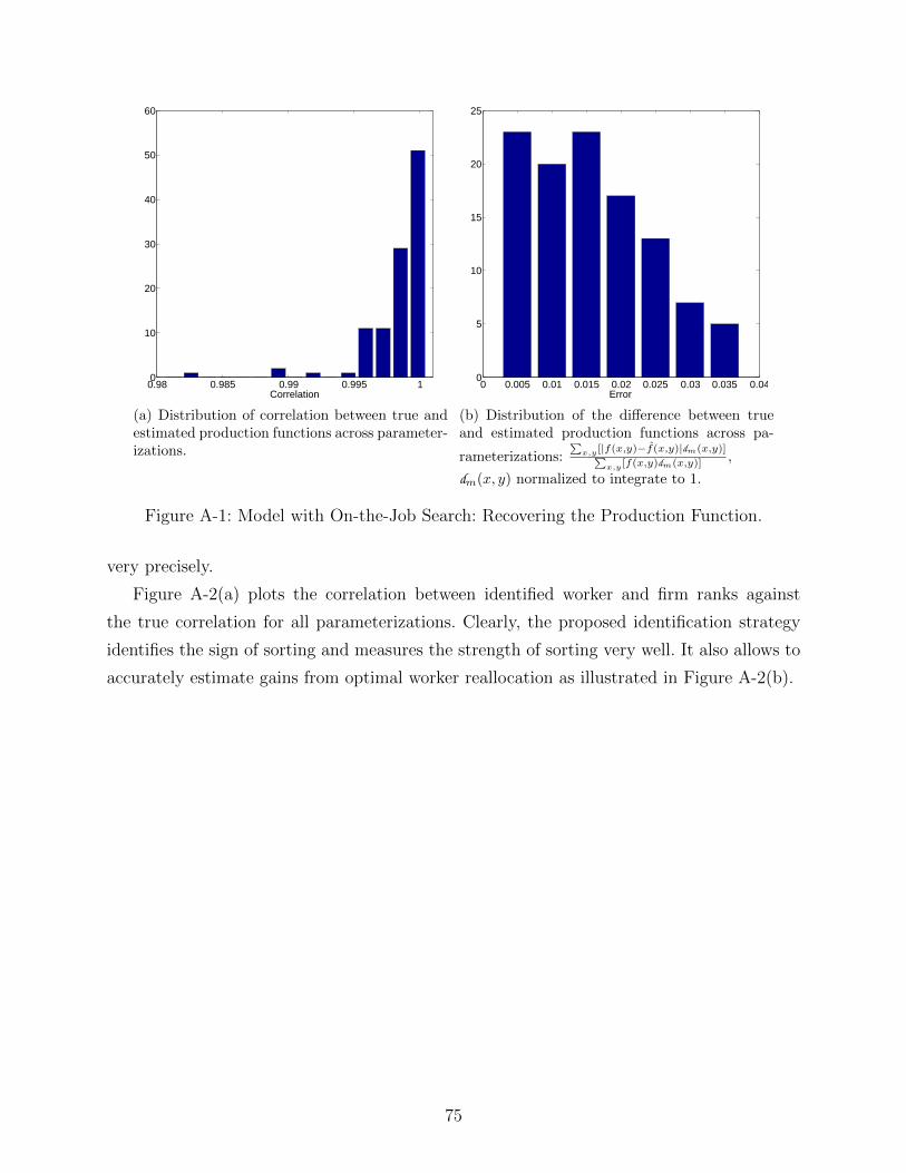
0.98 0.985 0.99 0.995 10
10
20
30
40
50
60
Correlation
(a) Distribution of correlation between true andestimated production functions across parameter-izations.
0 0.005 0.01 0.015 0.02 0.025 0.03 0.035 0.040
5
10
15
20
25
Error
(b) Distribution of the difference between trueand estimated production functions across pa-
rameterizations:∑
x,y [|f(x,y)−f(x,y)|dm(x,y)]∑x,y [f(x,y)dm(x,y)] ,
dm(x, y) normalized to integrate to 1.
Figure A-1: Model with On-the-Job Search: Recovering the Production Function.
very precisely.
Figure A-2(a) plots the correlation between identified worker and firm ranks against
the true correlation for all parameterizations. Clearly, the proposed identification strategy
identifies the sign of sorting and measures the strength of sorting very well. It also allows to
accurately estimate gains from optimal worker reallocation as illustrated in Figure A-2(b).
75
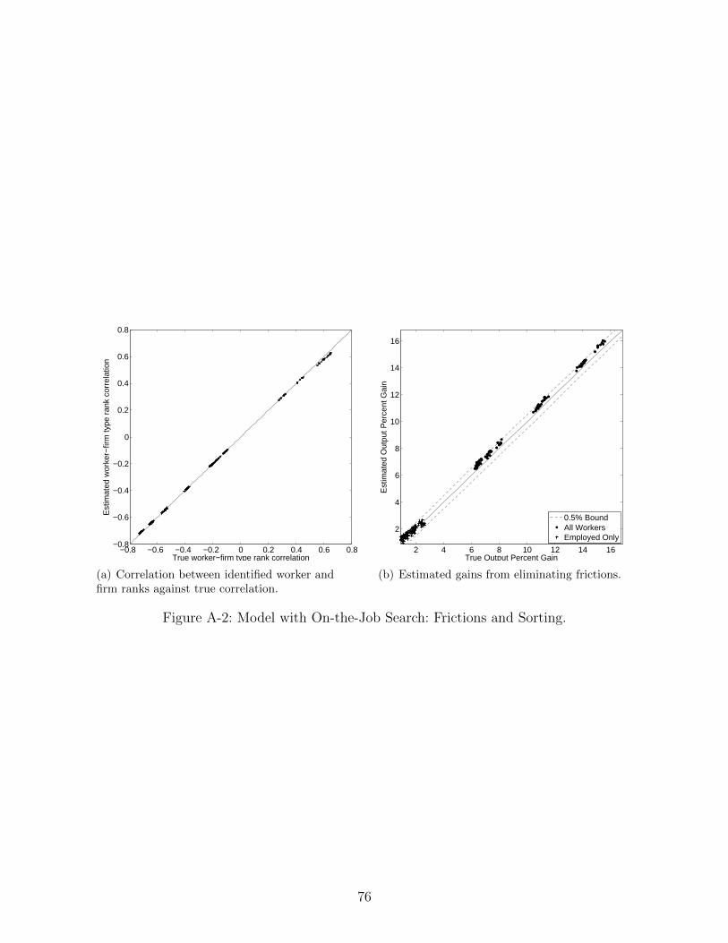
−0.8 −0.6 −0.4 −0.2 0 0.2 0.4 0.6 0.8−0.8
−0.6
−0.4
−0.2
0
0.2
0.4
0.6
0.8
True worker−firm type rank correlation
Est
imat
ed w
orke
r−fir
m ty
pe r
ank
corr
elat
ion
(a) Correlation between identified worker andfirm ranks against true correlation.
2 4 6 8 10 12 14 16
2
4
6
8
10
12
14
16
True Output Percent Gain
Est
imat
ed O
utpu
t Per
cent
Gai
n
0.5% BoundAll WorkersEmployed Only
(b) Estimated gains from eliminating frictions.
Figure A-2: Model with On-the-Job Search: Frictions and Sorting.
76

V Details of Empirical Analysis
As explained in the main text, our empirical work closely follows Card et al. (2013). Here,
we provide basic details and explain all the differences.
Our raw LIAB data contain employment histories of 2,087,683 German males aged 16 and
above observed working in 1,168,301 unique establishments. The worker data is continuous
(up to a day), and is based on notifications submitted by employers to various social insurance
agencies upon a change in the conditions of employment. The data include 34,263,798 spells
from the Employment History (Beschaftigten-Historik - BeH), which cannot be longer than
a year since an annual notification is required for all jobs in progress on December 31; and
6,488,810 spells from the Benefit Recipient History (Leistungsempfanger-Historik - LeH),
which can span multiple years.
Our analysis is based on daily wages in the main job of West German male workers age
20-60. While the data is continuous, we aggregate it to monthly frequency. In case of several
concurrent jobs in a given calendar month, we define the main one to be the job in which the
worker earns the most in that month. We drop all spells from the Benefit Recipient History,
spells with real (2005 base) daily earnings below 10 Euro, as well as spells that correspond
to individuals in training or working from home. We also drop several individuals with
over 150 employment spells. After this initial data preparation, we are left with 698,374
establishments, 1,973,679 workers and 22,675,589 employment spells.
Wages are censored at the social security maximum. We follow Dustman et al. (2009) and
impute censored wages by multiplying the censoring threshold by 1.2.45 Our identification
strategy is based on wages of workers who start new employment cycles, i.e individuals (1)
who start their first ever job, (2) whose start of a new job is preceded by compensated
unemployment, or (3) who have an uncompensated gap between two jobs longer than one
month. Only 2.41% of spells in this sample are censored.
To construct residual wages we follow Card et al. (2013). In particular, we regress in-
dividual log real daily wage yit of individual i in month t on a worker fixed effect αi and
an index of time-varying observable characteristics x′itβ which include an unrestricted set of
year dummies as well as a quadratic and cubic terms in age fully interacted with educational
attainment:
yit = αi + x′
itβ + rit,
45Card et al. (2013) use a different algorithm in Dustman et al. (2009) and stochastically impute censoredwages using a series of Tobit models. One argument of their Tobit model is the censoring rate of an individual’scoworkers. It is not possible to reliably construct this variable in LIAB data for establishments outside ofthe Establishment Panel because not all workers employed in those establishments are observed.
77

where rit is an error component. The residual wage which serves as input into the analysis
is then defined as wit = exp(yit − x′itβ).46
Having constructed wit, we rank workers. The ranking algorithm uses all available pair-
wise wage comparisons of workers who start employment cycles within an establishment
and does not require that all workers in the establishment are observed. Thus, we include
the comparisons in all establishments available in the LIAB data regardless of whether they
belong to the Establishment Panel.47 On this sample we also measure the labor market
transition rates.
After the ranking of workers has been constructed, we drop all establishments for which
we do not observe all workers (those that are not in the IAB Establishment Panel). We
also drop the establishments that employ less than 20 workers on average during the sample
period. This leaves us with a sample of 1,328,402 workers and 5,349 establishments. This
generates 13,381,974 employment-year spells of which 2,857,275 are out of unemployment.
Establishments in this sample are ranked following the procedure in Appendix IV.2.3. Fol-
lowing this, the production function is recovered.
46Card et al. (2013) also include establishment fixed effects in the regression. This difference is in-consequential for our purposes as the inclusion of establishment fixed effects has virtually no impacton β. In particular, corr(x
′
itβ, x′
itβCHK) = 0.9925 and corr(log(wit), log(wit,CHK)) = 0.9993, where
wit,CHK = exp(yit − x′
itβCHK).47Even restricting the pairwise connections to workers hired out of unemployment into the same firms
implies a highly connected set of workers. In particular, the largest connected set on this sample contains98.75% of workers. This is only a small reduction in connectedness relative to the full sample where thelargest connected set contains 99.81% of workers.
78

VI Appendix Figures
VI.1 Figures: Benchmark Model
0.2 0.3 0.4 0.50
2
4
6
8
10
12
14
Job Finding Rate0.02 0.04 0.06 0.080
2
4
6
8
10
12
14
16
18
Unemployment0.1 0.12 0.14 0.16
0
5
10
15
20
Variance log(Wages)
Figure A-3: Distributions of selected variables of interest across all parameterizations.
0.96 0.97 0.98 0.99 10
5
10
15
20
25
30
Minimum Wage0.96 0.97 0.98 0.99 10
5
10
15
20
25
30
Maximum Wage0.96 0.97 0.98 0.99 10
5
10
15
20
25
30
Adjusted Average Wage
Figure A-4: Distribution of the correlation between the true and estimated, using indicated
alternative ranking procedures, worker ranks across all parameterizations.
79

Figure A-5: True and estimated PAM production function.
Figure A-6: True and estimated NAM production function.
80

Figure A-7: True and estimated Neither NAM nor PAM production function.
81
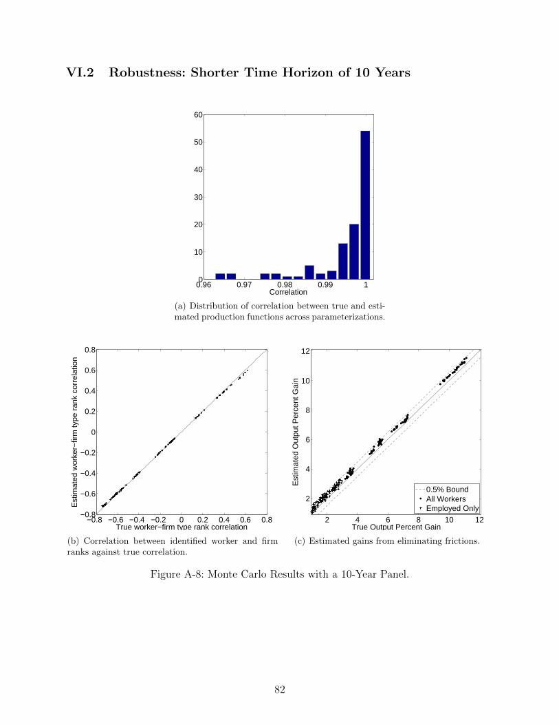
VI.2 Robustness: Shorter Time Horizon of 10 Years
0.96 0.97 0.98 0.99 10
10
20
30
40
50
60
Correlation
(a) Distribution of correlation between true and esti-mated production functions across parameterizations.
−0.8 −0.6 −0.4 −0.2 0 0.2 0.4 0.6 0.8−0.8
−0.6
−0.4
−0.2
0
0.2
0.4
0.6
0.8
True worker−firm type rank correlation
Est
imat
ed w
orke
r−fir
m ty
pe r
ank
corr
elat
ion
(b) Correlation between identified worker and firmranks against true correlation.
2 4 6 8 10 12
2
4
6
8
10
12
True Output Percent Gain
Est
imat
ed O
utpu
t Per
cent
Gai
n
0.5% BoundAll WorkersEmployed Only
(c) Estimated gains from eliminating frictions.
Figure A-8: Monte Carlo Results with a 10-Year Panel.
82

VI.3 Robustness: Small Firms
0.96 0.97 0.98 0.99 10
5
10
15
20
25
30
35
40
45
50
Correlation
(a) Distribution of correlation between true and esti-mated production functions across parameterizations.
−0.8 −0.6 −0.4 −0.2 0 0.2 0.4 0.6 0.8−0.8
−0.6
−0.4
−0.2
0
0.2
0.4
0.6
0.8
True worker−firm type rank correlation
Est
imat
ed w
orke
r−fir
m ty
pe r
ank
corr
elat
ion
(b) Correlation between identified worker and firmranks against true correlation.
2 4 6 8 10 12
2
4
6
8
10
12
True Output Percent Gain
Est
imat
ed O
utpu
t Per
cent
Gai
n
0.5% BoundAll WorkersEmployed Only
(c) Estimated gains from eliminating frictions.
Figure A-9: Monte Carlo Results with Maximum Firm Size of 20 Workers.
83

VI.4 Robustness: Stochastic Match Quality
0.985 0.99 0.995 10
5
10
15
20
25
30
35
40
Correlation
(a) Distribution of correlation between true and esti-mated production functions across parameterizations.
−0.6 −0.4 −0.2 0 0.2 0.4−0.6
−0.4
−0.2
0
0.2
0.4
True worker−firm type rank correlation
Est
imat
ed w
orke
r−fir
m ty
pe r
ank
corr
elat
ion
(b) Correlation between identified worker andfirm ranks against true correlation.
2 4 6 8 10 12 14
2
4
6
8
10
12
14
True Output Percent Gain
Est
imat
ed O
utpu
t Per
cent
Gai
n
0.5% BoundAll WorkersEmployed Only
(c) Estimated gains from eliminating frictions.
Figure A-10: Monte Carlo Results on a Model with Stochastic Match Quality.
84
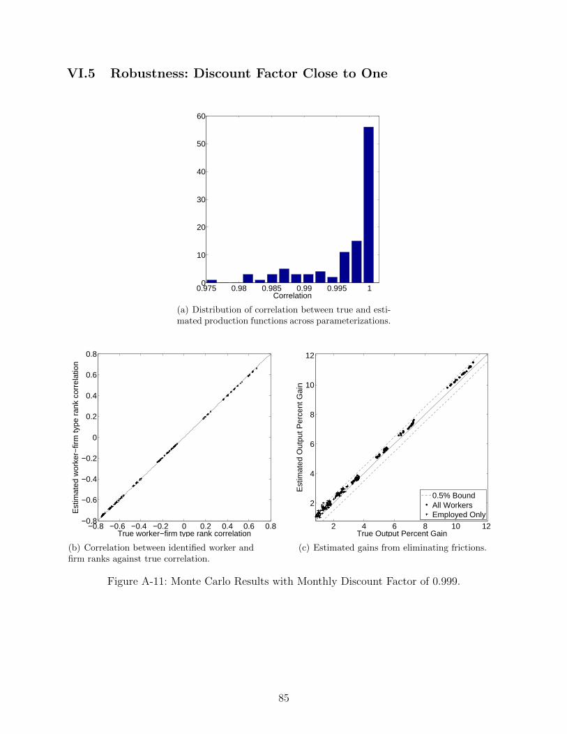
VI.5 Robustness: Discount Factor Close to One
0.975 0.98 0.985 0.99 0.995 10
10
20
30
40
50
60
Correlation
(a) Distribution of correlation between true and esti-mated production functions across parameterizations.
−0.8 −0.6 −0.4 −0.2 0 0.2 0.4 0.6 0.8−0.8
−0.6
−0.4
−0.2
0
0.2
0.4
0.6
0.8
True worker−firm type rank correlation
Est
imat
ed w
orke
r−fir
m ty
pe r
ank
corr
elat
ion
(b) Correlation between identified worker andfirm ranks against true correlation.
2 4 6 8 10 12
2
4
6
8
10
12
True Output Percent Gain
Est
imat
ed O
utpu
t Per
cent
Gai
n
0.5% BoundAll WorkersEmployed Only
(c) Estimated gains from eliminating frictions.
Figure A-11: Monte Carlo Results with Monthly Discount Factor of 0.999.
85


![Identifying Sorting - In Theory · Identifying Sorting - In Theory ... Workers draw their type xfrom distribution Γ(x) with smooth density γ(x) on [0,1].Firms draw their type yfrom](https://img.pdfslide.us/doc/110x75/5ec38b809df52b6207504728/identifying-sorting-in-theory-identifying-sorting-in-theory-workers-draw.jpg)