An asymptotic approach to inverse scattering problems on ... fileAn asymptotic approach to inverse scattering problems on

AN ASYMPTOTIC APPROACH TO INVERSESCATTERING PROBLEMS ON WEAKLYNONLINEAR ELASTIC RODS

SHINUK KIM AND KEVIN L. KREIDER

Received 27 September 2001 and in revised form 28 May 2002

Elastic wave propagation in weakly nonlinear elastic rods is consideredin the time domain. The method of wave splitting is employed to for-mulate a standard scattering problem, forming the mathematical basisfor both direct and inverse problems. A quasi-linear version of theWendroff scheme (FDTD) is used to solve the direct problem. To solvethe inverse problem, an asymptotic expansion is used for the wave field;this linearizes the order equations, allowing the use of standard numer-ical techniques. Analysis and numerical results are presented for threemodel inverse problems: (i) recovery of the nonlinear parameter in thestress-strain relation for a homogeneous elastic rod, (ii) recovery of thecross-sectional area for a homogeneous elastic rod, (iii) recovery of theelastic modulus for an inhomogeneous elastic rod.

1. Introduction

Wave propagation in nonlinear elastic and viscoelastic materials hasbeen an area of interest for some time. There has been an extensiveamount of work done on the mathematical modeling of such materials(e.g., [2, 10, 17, 19, 20, 23]), as well as on the analysis of the behavior ofspecific materials (e.g., [11, 21, 26]). These efforts fall into two classes:the modeling of the stress-strain relation, usually in conjunction withcurve fitting to experimental data, and the modeling of wave propaga-tion in nonlinear media, both in the time domain and in the frequencydomain. A few application areas include seismic imaging for oil explo-ration, structural dynamics, and nondestructive evaluation.

Copyright c© 2002 Hindawi Publishing CorporationJournal of Applied Mathematics 2:8 (2002) 407–4352000 Mathematics Subject Classification: 74J30, 74B20, 74H10, 74J25, 65M32, 41A60URL: http://dx.doi.org/10.1155/S1110757X0210903X

http://dx.doi.org/10.1155/S1110757X0210903X

408 Inverse scattering on weakly nonlinear rods

Extensive work has been done on inverse problems for linear materi-als [4, 5, 7, 9, 12]. However, the literature on inverse problems for non-linear rods is sparse [8, 13, 18, 22, 24], especially in the time domain (al-though there has been recent activity in nonlinear electromagnetic scat-tering problems using wave splitting [1, 6, 16, 25]). But the time domainis the natural place to study the propagation of short duration pulses,nonperiodic waves and transients, which are important in many applica-tions. Therefore, it is important to develop analytic and numerical toolsto examine the time dependent behavior of nonlinear elastic waves. Aprogram of such study was recently begun [8], and further developed in[13].

It is convenient to begin the study of wave propagation in nonlinearelastic media with the study of one-dimensional rods of finite length d,as is done here. This makes the wave splitting analysis tractable, and stillprovides insight into meaningful applications.

1.1. Goals of the paper

At present, it is not clear how best to solve inverse scattering problemsin nonlinear rods. An optimization approach was presented in [8]. Thispaper presents an alternative, a simple asymptotic approach for weaklynonlinear elastic rods. There are two goals here. First, the long range in-tent is to determine, by numerical experimentation, the conditions forwhich this approach yields reasonable results for some typical inverseproblems, in order to provide insight into how to approach inverse prob-lems on any nonlinear rod. Indeed, the authors are beginning an exten-sive program of study of inverse problems for nonlinear elastic and vis-coelastic wave propagation in two-dimensional media, and work is cur-rently underway to improve the numerical implementation of both theoptimization and asymptotic approaches, and to search for other feasiblemethodologies. Second, the immediate intent is to develop an analyticalframework for the asymptotic approach so that higher-order correctionscan be incorporated into the analysis presented here. It is reasonable topresume that including higher-order corrections could allow the asymp-totic approach to resolve inverse problems involving stronger nonlinear-ities, significantly enhancing the utility of the approach.

The remainder of the paper is organized as follows. Section 2 presentsthe model problem under consideration. Section 3 outlines the mathe-matical formulation of scattering problems using wave splitting. Thesystem of equations used in numerical work appears at the end of thesection. Section 4 describes the implementation of the direct algorithm.Section 5 contains a brief description of the inverse problems to be con-sidered. In Section 6, there appears the analysis and numerical results forthe case of the homogeneous nonlinear elastic rod; the inverse problem

S. Kim and K. L. Kreider 409

is to recover the value of the nonlinear parameter b1. Section 7 discussesanalysis and numerical results for the case of the homogeneous nonlin-ear elastic rod with varying cross section. The inverse problem is to re-cover the cross-sectional area. Section 8 contains analysis and numericalresults for the case of the inhomogeneous elastic rod. The inverse prob-lem is to recover the elastic modulus. Section 9 contains a summary ofthe techniques and results.

2. Physical model

Consider an infinite nonlinear rod with a slab of nonlinear elastic mate-rial lying in x ∈ [0,d]. The material properties (density ρ, elastic modu-lus E, and cross-sectional area A) are constant outside the slab, and varycontinuously for all x. In particular, there are no jump discontinuities atx = 0 or x = d. The stress-strain relation is assumed to have the form

σ(x,t) = F(x,ε(x,t)

)= E(x)

(ε(x,t) + b1ε

2(x,t))

(2.1)

or

σ = F(ε) = E(ε + b1ε

2). (2.2)

For purposes of illustration, a quadratic nonlinearity (F(x,ε)=E(ε+b1ε2))

is presented, although the analysis below could be generalized to otherforms of F(x,ε) if desired. An important assumption in this paper isthat the material is weakly nonlinear, which means that |b1| is small. Thevalue of b1 can be positive or negative, although for most elastic solids,b1 is negative.

The equation of motion and the compatibility relation are

∂tv(x,t) =1

ρ(x)A(x)∂x(A(x)σ(x,t)

), ∂xv(x,t) = ∂tε(x,t), (2.3)

where v(x,t) is particle velocity. This leads to the system of equations

∂xv = ∂tε,

∂tv =1Aρ

(A′σ +A

[E′(ε+ b1ε

2)+E(∂xε + 2b1ε∂xε

)])=

1ρ

(E(1+ 2b1ε

)∂xε+

A′

AF(ε) +E′(ε+ b1ε

2))

=1ρG(x,ε)∂xε+M(x,t),

(2.4)


where M includes the effects of spatial inhomogeneity and G ultimatelyaffects the speed of waves traveling through the rod in nonlinear fashion

M(x,t) =1

ρ(x)

(A′(x)A(x)

F(x,ε(x,t)

)+E′(x)

[ε(x,t) + b1ε(x,t)

]),

G(x,ε(x,t)

)= E(x)

(1+ 2b1ε(x,t)

).

(2.5)

This system, along with suitable boundary and initial conditions (pre-sented in the next section), forms the mathematical basis for scatteringproblems on a nonlinear rod.

3. Problem formulation

In this section, the method of wave splitting is used to put the system(2.4), into a form suitable for numerical computations. This methodol-ogy was developed in [8], and is summarized here for convenience.

First, write (2.4) in matrix form as

(√G/ρ∂tε

∂tv

)=(

0√G/ρ√

G/ρ 0

)(√G/ρ∂xε

∂xv

)+

(0M

). (3.1)

It must be assumed that G > 0. For sufficiently small strains, this is notrestrictive, since it is reasonable to expect the stress to increase as thestrain increases. The system is simplified by defining

g(x,ε) =∫ε

0

√G(x,ε′)ρ(x)

dε′ =

√E(x)ρ(x)

∫ε

0

√1+ 2b1ε′dε′

=1

3b1r(x)[(

1+ 2b1ε)3/2 − 1

],

r(x) =

√ρ(x)E(x)

(3.2)

and introducing new dependent variables

u1(x,t) = g(x,ε(x,t)

), u2(x,t) = v(x,t). (3.3)


For fixed x, g is strictly increasing with respect to ε, so there existsan inverse g−1, interpreted as ε = g−1(x,u1) = (1/2)b1[(1+ 3b1ru1)2/3 − 1].The system is now represented as

∂t

(u1

u2

)=(

0 cc 0

)∂x

(u1

u2

)+

(0N

)(3.4)

with N and wave speed c defined by

N =M− c∂xg =M− cd

dx

(√E

ρ

)∫ε

0

√1+ 2b1ε′dε′,

c(x,u1

)=

1∂u1g

−1(x,u1

) = 1r(x)

(1+ 3b1r(x)u1

)1/3.

(3.5)

It must be assumed that 1+ 3b1ru1 > 0 for the wave speed to be nonneg-ative.

The wave splitting transformation is introduced in order to diagonal-ize the wave speed matrix. New dependent variables are defined by

(u+

u−

)= P

(u1

u2

),

(u1

u2

)= P−1

(u+

u−

), (3.6)

where

P =12

(1 −11 1

), P−1 =

(1 1−1 1

). (3.7)

This final change of variables yields the quasi-linear equations of mo-tion

∂tu± ± c∂xu

± = ∓N2. (3.8)

If the material is spatially inhomogeneous, it is advantageous to intro-duce travel time coordinates in order to straighten the curve for the lead-ing edge in the space-time plane. This makes it easier to set up a discretegrid for numerical work. The speed of the wave front is denoted cτ(x).The travel time of the wave front for traversing the rod from x = 0 tox = d is

� =∫d

0

dx′

cτ(x′). (3.9)


The travel time coordinate transformation is then

x(x) =1�

∫x

0

dx′

cτ(x′), t =

t

�. (3.10)

At this point, the dynamic equations can be nondimensionalized, drop-ping tildes, as

∂tu± ± cn∂xu

± = ∓N2

(3.11)

with cn = c/cτ . Under this scaling, the wave speed along the leadingedge is normalized to 1. The explicit forms of the nondimensional co-efficients are

cτ(x,u+,u−) = 1

r

(1+ 3b1ru

+)1/3,

cn(x,u+,u−) =(1+ 3b1r

[u+ +u−]

1+ 3b1ru+

)1/3

,

N =1cτρ

[A′

AF(ε) +E′(ε + b1ε

2)+ ρcr ′[u+ +u−]r

].

(3.12)

At x = 0, an incident velocity v(0, t) = f(t) is applied, so that the bound-ary condition is f(t) = −u+(0, t) +u−(0, t). Casuality implies that all fieldsvanish before the time of first arrival, so that u±(x,t) = 0 for x > t. Thisis the formulation used for the direct and inverse scattering problemsconsidered below.

3.1. Summary of assumptions

In the analysis presented above, two assumptions are needed to ensurethat the formulation is physically meaningful. First, it is necessary thatG > 0 for the wave splitting variables to remain real. This means that 1+2b1ε(x,t) > 0, which implies that the strain field ε remains small in mag-nitude. The value of ε can be positive (the rod is in extension) or negative(the rod is in compression). If b1 > 0, then ε > −1/2b1, which means therod can be in extension or slight compression. If b1 < 0, then ε < −1/2b1 =1/2|b1|, which means the rod can be in compression or slight extension.

Second, it is necessary that (1 + 3b1ru1) > 0 for the wave speed to re-main nonnegative. The split field u1 = u+ +u− = g can be positive or neg-ative. If b1 > 0 then u1 > −1/(3b1r), while if b1 < 0 then u1 < 1/(3|b1|r).

The assumption that |b1| is small is not necessary here, but does makethese inequalities more easily satisfied; the assumption is used in latersections to develop asymptotic algorithms for inverse problems.


Figure 4.1. Numerical grid for the direct algorithm. Circles indicategrid points, and the dynamic equations are applied at cell centers,indicated by ×.

4. The direct problem

A quasi-linear version of the Wendroff scheme [3] is applied to the dy-namic equations (3.11), in which the partial derivatives are discretized as

∂xu±i+1/2,j+1/2 =

12

(u±i+1,j+1 −u±

i,j+1

h+u±i+1,j −u±

i,j

h

),

∂tu±i+1/2,j+1/2 =

12

(u±i+1,j+1 −u±

i+1,j

h+u±i,j+1 −u±

i,j

h

).

(4.1)

For linear equations (cn is constant), the scheme is second order, witherror O(∆x2 +∆t2), and is unconditionally stable. There is no theory topredict the stability properties of the quasi-linear form, but no numeri-cal difficulties have appeared in the problems under consideration hereduring extensive testing.

This discretization leads to an implicit scheme, the result of which isa coupled system along each time line tj . The unknowns {u±

i,j , i = 1, . . . ,j − 1} are obtained one row at a time. Leading edge values u±

jj are com-puted earlier, as described below. Figure 4.1 shows the grid schematicfor an arbitrary row. The dynamic equations are applied at the cell cen-ters, indicated by an ×, providing 2j − 2 equations. The system is closedby including the boundary condition fj = −u+

0j + u−0j and the directional

derivative of u− at the leading edge, obtained from the dynamic equationfor u− : u−

j−1,j = u−j−1/2,j−1/2 + (h/2)Nj−1/2,j−1/2/2 = (h/4)Nj−1/2,j−1/2.


The presence of the nonlinear factors N and cn complicates the anal-ysis; these factors should be evaluated at cell centers (xi+1/2, tj+1/2), pre-sumably by averaging the values of u+ and u− at the four surroundinggrid points. But this leads to a nonlinear system along time line t = tjbecause u±

i,j and u±i+1,j are unknown. Since the material is assumed to

be weakly nonlinear, this difficulty can be avoided by averaging theknown values of u+ and u− at the two lower grid points (i, j − 1) and(i+ 1, j − 1).

The quasi-linear direct algorithm is used to create synthetic reflectionand transmission data to be used as inputs in the inverse problems pre-sented below.

5. Three inverse problems

Three inverse problems considered in this paper are the following.(1) The homogeneous elastic rod. The cross-sectional area A(x) = 1,

the constant density ρ, and constant elastic modulus E are known. Thegoal is to recover the nonlinear parameter b1.

(2) The rod with varying cross section. The density, modulus, andnonlinear parameter are known. The goal is to recover the cross-sectionalarea A(x).

(3) The rod with varying modulus. The density, cross section, andnonlinear parameter are known. The goal is to recover the modulusE(x).

Figure 5.1 contains pictures of the rods and the computational do-mains for each problem.

In general, we would expect these inverse problems for nonlinear ma-terials to be ill-posed. However, if |b1| is sufficiently small, then eachof the inverse problems has a unique solution. Sketches of the proofsare presented in the appropriate Sections 6.3, 7.4, and 8.3. Although thedetails differ from one problem to another, there are two basic themes:the linearized problem has a unique solution if the coefficients are suffi-ciently smooth and the inputs are sufficiently small, and the higher-orderterms in the asymptotic expansion are continuous on the computationaldomains (Figure 5.1) and so are uniformly bounded.

6. The homogeneous elastic rod

In this section, the inverse problem for the nonlinear homogeneous elas-tic rod is formulated, a discussion on uniqueness of solution for the in-verse problem is presented, the inverse algorithm is developed, and nu-merical results are presented and discussed; this material was first de-scribed in [13].


(a)

10.80.60.40.200

0.5

1

1.5

2

(b)

(c)

10.80.60.40.200

0.5

1

1.5

2

(d)

Figure 5.1. Rod geometries and computational domains for thethree inverse problems under consideration. (a) Rod geometry forthe homogeneous rod and the rod with varying modulus. (b) Com-putational domain for the homogeneous rod, {(x,t) | 0 ≤ x ≤ 1, x ≤t ≤ x + 1}. (c) Rod geometry for the rod with varying cross-sectionalarea. (d) Computational domain for the rod with varying cross-sectional area and the rod with varying modulus, {(x,t) | 0 ≤ x, x ≤t ≤ 2−x}.

6.1. Analytic formulation

The nonlinear homogeneous elastic rod is the simplest nonlinear rod.The density ρ and modulus E are constant, so that r(x) can be scaled to 1.Because there are no spatial inhomogeneities, the dynamic equations


simplify, considerably,

∂t

(u+

u−

)=(−cn(u+ +u−) 0

0 cn(u+ +u−)

)∂x

(u+

u−

). (6.1)

The nonlinear wave speed cn couples the two equations. However,there is no local coupling between u+ and u− due to material inhomo-geneities, so if no external left-going field (u−) is applied, then the fieldis entirely right-going, so u− ≡ 0, and the dynamic equations reduce to ascalar equation in u+ as

∂tu+ + cn

(u+)∂xu+ = 0. (6.2)

Note that the wave speed cn(u+) still depends on the field magnitude,and hence the problem is still nonlinear. Also, the boundary conditionsimplifies to u+(0, t) = −f(t) = −v(0, t).

It is convenient to devise a scattering experiment in which the appliedparticle velocity at the boundary has the property that f(0) = 0; this im-plies that u+ = 0 along the leading edge, so that the wave front speed cτ =1 and cn = c = (1 + 3b1u

+)1/3. The incident velocity v(0, t) = f(t) = t2/2was used in the numerical experiments presented in Section 6.5. Thisfunction was chosen because it offers a smooth, linearly increasing ac-celeration, which models a linearly increasing force applied to the endof the rod. Because the time interval of interest is [0,1], there is no issuewith the fact that the velocity function is monotonically increasing.

The inverse problem here is to use transmission data, u+(1, t), to re-cover the nonlinear parameter b1. For notational convenience, write u+

as u. Straightforward asymptotic expansions of u and c in terms of b1,

u = u0 + b1u1 + b21u2 + · · · ,

c(u) =(1+ 3b1u

)1/3 = 1+ b1u− b21u

2 + · · ·(6.3)

can be applied, resulting in the order equations

O(1) : ∂tu0 + ∂xu0 = 0, (6.4)

O(b1)

: ∂tu1 + ∂xu1 = −u0∂xu0, (6.5)

O(b2

1

): ∂tu2 + ∂xu2 = −u0∂xu1 −

(u1 −u2

0

)∂xu0. (6.6)

The important feature in each of these equations is that the wave speedhas been linearized; in fact, due to the nondimensionalization, the wavespeed is normalized to 1. This means that each field ui propagates alonga straight characteristic with slope 1 in space-time coordinates, so that


the method of characteristics may be used to solve these equations ana-lytically, making the inverse algorithm much more simple. In addition,it should be noted that the cubic term b1u

3 was included in the asymp-totic expansion, but it was found that this term is so small that it has anegligible effect on the results.

Consider (6.4) for u0 along an arbitrary characteristic t = x + ξ. Theequation may be written as

du0

dt= 0, u0(0, ξ) = −f(ξ) (6.7)

which has solution

u0(t− ξ, t) = −f(ξ). (6.8)

Using ξ = t−x, it is easy to see that partial derivatives of u0 with respectto x on the curve t = x + ξ may be written as

∂xu0(t− ξ, t) = f ′(ξ). (6.9)

Consider (6.5) for u1 along the same characteristic t = x + ξ. The equa-tion may be written as

du1

dt= f(ξ)f ′(ξ), u1(0, ξ) = 0 (6.10)

which has solution

u1(t− ξ, t) = f(ξ)f ′(ξ)t. (6.11)

Using ξ = t−x, it is easy to see that partial derivatives of u1 with respectto x on the curve t = x + ξ may be written as

∂xu1(t− ξ, t) = −[(f ′(ξ))2 + f(ξ)f ′′(ξ)

]t. (6.12)

Consider (6.6) for u2 along the same characteristic t = x + ξ. The equa-tion may be written as

du2

dt= −[2f(ξ)(f ′(ξ)

)2 + f2(ξ)f ′′(ξ)]t+ f2(ξ)f ′(ξ), u2(0, ξ) = 0

(6.13)


which has solution

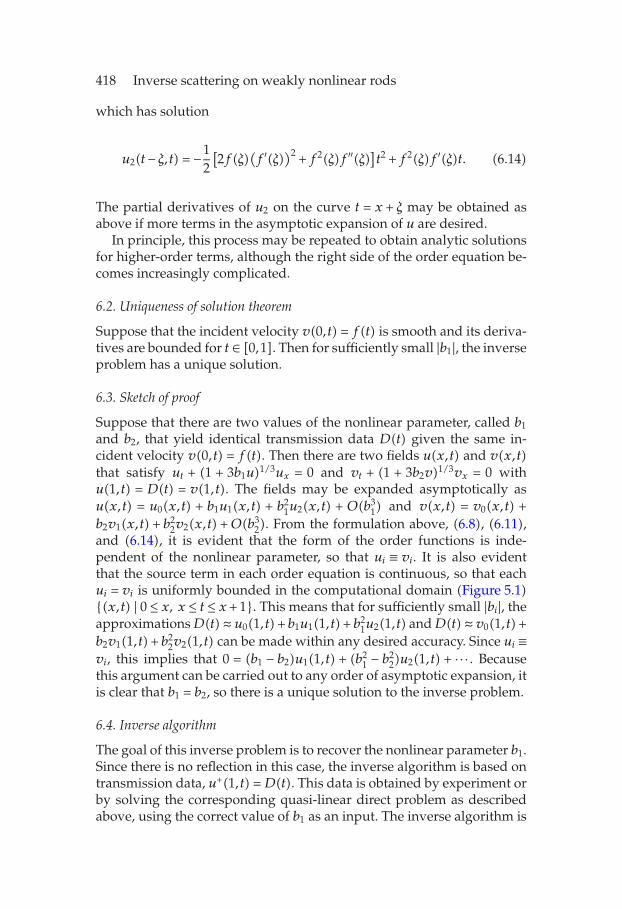
u2(t− ξ, t) = −12[2f(ξ)

(f ′(ξ)

)2 + f2(ξ)f ′′(ξ)]t2 + f2(ξ)f ′(ξ)t. (6.14)

The partial derivatives of u2 on the curve t = x + ξ may be obtained asabove if more terms in the asymptotic expansion of u are desired.

In principle, this process may be repeated to obtain analytic solutionsfor higher-order terms, although the right side of the order equation be-comes increasingly complicated.

6.2. Uniqueness of solution theorem

Suppose that the incident velocity v(0, t) = f(t) is smooth and its deriva-tives are bounded for t ∈ [0,1]. Then for sufficiently small |b1|, the inverseproblem has a unique solution.

6.3. Sketch of proof

Suppose that there are two values of the nonlinear parameter, called b1

and b2, that yield identical transmission data D(t) given the same in-cident velocity v(0, t) = f(t). Then there are two fields u(x,t) and v(x,t)that satisfy ut + (1 + 3b1u)1/3ux = 0 and vt + (1 + 3b2v)1/3vx = 0 withu(1, t) = D(t) = v(1, t). The fields may be expanded asymptotically asu(x,t) = u0(x,t) + b1u1(x,t) + b2

1u2(x,t) + O(b31) and v(x,t) = v0(x,t) +

b2v1(x,t) + b22v2(x,t) +O(b3

2). From the formulation above, (6.8), (6.11),and (6.14), it is evident that the form of the order functions is inde-pendent of the nonlinear parameter, so that ui ≡ vi. It is also evidentthat the source term in each order equation is continuous, so that eachui = vi is uniformly bounded in the computational domain (Figure 5.1){(x,t) | 0 ≤ x, x ≤ t ≤ x+ 1}. This means that for sufficiently small |bi|, theapproximations D(t) ≈ u0(1, t) + b1u1(1, t) + b2

1u2(1, t) and D(t) ≈ v0(1, t) +b2v1(1, t) + b2

2v2(1, t) can be made within any desired accuracy. Since ui ≡vi, this implies that 0 = (b1 − b2)u1(1, t) + (b2

1 − b22)u2(1, t) + · · · . Because

this argument can be carried out to any order of asymptotic expansion, itis clear that b1 = b2, so there is a unique solution to the inverse problem.

6.4. Inverse algorithm

The goal of this inverse problem is to recover the nonlinear parameter b1.Since there is no reflection in this case, the inverse algorithm is based ontransmission data, u+(1, t) =D(t). This data is obtained by experiment orby solving the corresponding quasi-linear direct problem as describedabove, using the correct value of b1 as an input. The inverse algorithm is


based on the least-squares curve fit approximation

D(t) ≈ u0(1, t) + b1u1(1, t) + b21u2(1, t). (6.15)

The transmission data is discretized at time steps tj , and is denoted Dj =D(tj). These data points are added, leading to the sum

S(b1)=

M∑j=0

(Dj −

[u0(1, tj)+ b1u1

(1, tj)+ b2

1u2(1, tj)])2

. (6.16)

Because analytic expressions for the ui are given in terms of the knownincident field f(t), the only unknown is b1, which can be obtained by astandard least squares approach.

6.5. Numerical results

A set of numerical experiments was used to gauge the algorithm’s over-all performance.

Test 1. How much of the transmission data should be used?

Notice that the asymptotic approximation (6.15) to D(t) is quadraticin time, due to the t2 factor in u2, so the least-squares fit will work bestin the short time, where D(t) is roughly quadratic. Under the travel timescaling, the wave travels through the material in scaled time t ∈ [0,1],and transmission data is obtained for this time interval. Let τ denote thefraction of this data that is used by the inverse algorithm. A numericalexamination of a variety of cases, with b1 ranging from −20 to 20, indi-cates that the best recovery of b1 occurs when τ < .05 (i.e., less than 5% ofthe data for one travel time is used), although for smaller values of |b1|,the value of τ does not appear to be crucial. A reasonable rule of thumbis to let τ = .04 for the inverse algorithm to give meaningful results.

Test 2. What is the effect of finite difference discretization error?

The inverse algorithm was run for a variety of b1 values using τ = .04with a spatial grid of n subintervals. Table 6.1 shows the computed val-ues of b1 for a variety of grids for actual values of b1 = ±.01,±.1,±1,±10.The results indicate that finer grids do provide better results, but whencomputation time is taken into account, the marginal cost is too high. Therecommended n value is 2048 for smaller |b1| values (roughly speaking,b1 ∈ (−5,5)), while it may be advantageous to use n = 4096 if |b1| is larger.

Test 3. What range of b1 values can be recovered?


Table 6.1. The effect of discretization error on the recovery of b1. Ineach section, the actual b1 value is given above, and the values beloware the computed values of b1 using the indicated number n of spatialgrid points.

n b1 = −.01 b1 = −.1 b1 = −1 b1 = −10

128 −.0078 −.0779 −.7805 −9.5911256 −.0086 −.0864 −.8657 −10.2594512 −.0091 −.0913 −.9150 −10.61101024 −.0094 −.0939 −.9416 −10.79732048 −.0095 −.0953 −.9552 −10.78254096 −.0096 −.0959 −.9621 −10.7733

n b1 = +.01 b1 = +.1 b1 = +1 b1 = +10

128 .0078 .0780 .7809 9.0220256 .0086 .0864 .8652 10.2093512 .0091 .0913 .9140 10.89941024 .0094 .0939 .9403 11.28262048 .0095 .0953 .9538 11.54484096 .0096 .0959 .9606 11.6797

The inverse algorithm was run with n = 2048 and τ = .04 to determinethe range of b1 values for which the relative error is less than 5% or 10%.To stay within a 10% error bound, the value of b1 must be in the interval(−12.25,8.75), and to stay within a 5% error bound, the value of b1 mustbe in the interval (−5.5,7.25).

These results clearly indicate that the methodology is useful only forsmall values of b1, and a different technique must be used to analyzestrongly nonlinear materials.

Because this problem requires derivatives of the incident field f(t),care must be exercised in specifying a continuous, differentiable inci-dent field. Jumps in f or its derivatives can significantly affect the perfor-mance of the algorithm. For example, with the actual value b1 = −.1, andn = 512 and τ = .40, the algorithm yields the computed value b1 = −.0838for the incident field f(t) = −t2/2. When this incident field is modifiedto be equal to .02 for t > .2 (so that f is continuous but f ′ has a jump att = .2), the computed result is b1 = −.0804, a slight degradation in solu-tion. When a jump is introduced into the incident field (f(t) = t2/2 fort < .2 and f(t) = .5 for t ≥ .2), the algorithm yields b1 = 1.831, which isclearly unacceptable.


Overall, the three tests indicate that the recovery of b1 is reasonablefor small values of b1, but that this algorithm has a limited usefulness ingeneral.

7. An inverse problem for the elastic rod with varying cross section

In this section, the inverse problem for the nonlinear homogeneous elas-tic rod with varying cross-sectional area is formulated, the inverse al-gorithm is developed, a discussion of uniqueness of solution for the in-verse problem is presented, and numerical results are presented and dis-cussed; this was first described in [13].


For this problem, the stress-strain relation is again taken to be

σ = F(x,ε) = E(x)(ε + b1ε

2), (7.1)

where |b1| < 1 and the scalings ρ = 1, E = 1 are used. The dynamic equa-tions take the form

∂t

(u+

u−

)=

(−cn(u++u−) 00 cn

(u++u−)

)∂x

(u+

u−

)+

(−α(x)F(ε)α(x)F(ε)

),

(7.2)

where α(x) = (1/2)A′(x)/A(x), and the nonlinear wave speed cn andnonlinear source term F couple the two equations. The leading terms ofthe asymptotic expansion of u+ and u− satisfy

∂tu+0 + ∂xu

+0 = −α(u+

0 +u−0

), (7.3)

∂tu−0 − ∂xu

−0 = +α

(u+

0 +u−0

). (7.4)

As in the previous example, the wave speed has been linearized, butthe equations remained coupled. This means that the inverse algorithmfor the homogeneous rod cannot be used, because analytic expressionsfor u±

0 are no longer available. A different approach must be taken.


Consider the recovery of A(x) from reflection data u−(0, t) =D(t) with-out knowledge of b1. The reflection data is obtained by solving the directproblem, using the correct values of b1 and A(x) as inputs. Then, the


leading order equations (7.3) and (7.4) are solved numerically to obtainthe values of A(xi) at each spatial grid point. The main source of errorin this algorithm, which is described below, is that the input data D(t)has not been linearized. Therefore, the method is appropriate only forweakly nonlinear materials, for which the correction terms (u1, u2,...)may be safely ignored.

For notational convenience, denote u±0 as u±. The inverse problem is

specified as follows: the dynamic equations (7.3) and (7.4) are combinedwith boundary conditions

u+(0, t) =D(t)− f(t), u−(0, t) =D(t) (7.5)

and leading edge conditions

u+(x,x+) = −A1/2(0)A1/2(x)

f(0), (7.6)

u−(x,x+) = 0, (7.7)

where f(t) = v(0, t) is the known incident field and D(t) is the reflec-tion data, to form a well-posed problem. Note that it is necessary thatf(0) = 0 because the leading edge condition is used to recover A(x). Forthis reason, the initial velocity v(0, t) = f(t) = 1 + t was chosen for thiscase, as a matter of convenience.

The leading edge conditions are derived from a propagation of dis-continuities argument. First, the curve t = x is not a characteristic for u−,so u− cannot admit a discontinuity along that curve. Since u− = 0 for x > tby causality, it must therefore be zero along the leading edge. However,t = x is a characteristic for u+, so there may be a discontinuity in u+ alongthe leading edge. Consider (7.3) for t = x+ and t = x−, and subtract thetwo to get an equation for the jump in u+, denoted [u+]

d

dx

[u+] = −α(x)([u+]+ [u−]). (7.8)

Along t = x, this is an ordinary differential equation with [u−] = 0, whichhas solution given by (7.6).

The inverse algorithm is a finite difference approach to the methodof characteristics. First, discretize the domain by letting ∆x = h, ∆t = 2h,with h = 1/N for some integer N, so that xi = (i− 1)h for i = 1, . . . ,N + 1,and tj = 2(j − 1)h for j = 1, . . . ,N + 1. Note that tj is measured in wavefront time; that is, it is the time after the first arrival of the wave front.


The absolute time at spatial location xi is given by xi + tj . The grid pointsare numbered so that the leading edge corresponds to j = 1, with highervalues of j representing later right-moving characteristics, given by t =x + tj . This grid should be consistent with that used in the direct problem,so that the values D(tj) are easily accessible.

To obtain equations valid at grid location (i, j), apply forward differ-encing at (i− 1, j) and backward differencing at (i, j) to the u+ equation,(7.3), and add, to obtain

2h

(u+i,j −u+

i−1,j

)= −αi−1

(u+i,j +u−

i−1,j

)−αi

(u+i,j +u−

i,j

). (7.9)

Then apply forward differencing at (i − 1, j + 1) and backward differ-encing at (i, j) to the u− equation, (7.4), and add, to obtain

2h

(u−i,j −u−

i−1,j+1

)= −αi−1

(u+i−1,j+1 +u−

i−1,j+1

)−αi

(u+i,j +u−

i,j

). (7.10)

Taking values at spatial location i − 1 to be known, (7.9) and (7.10)form a 2× 2 system in unknowns u+

i,j and u−i,j , which can be easily solved

to give

(u+i,j

u−i,j

)=

1(2/h)

(2/h+ 2αi

)

2h+αi −αi

−αi2h+αi

(R1

R2

), (7.11)

where

R1 =(

2h

)u+i−1,j −αi−1

(u+i−1,j +u−

i−1,j

),

R2 =(

2h

)u−i−1,j+1 −αi−1

(u+i−1,j+1 +u−

i−1,j+1

).

(7.12)

Equation (7.11) is valid at any interior point in the grid (not on theboundary i = 1 or the leading edge j = 1).

To determine the leading edge conditions at j = 1, use (7.4). Applybackward differencing at (i,1) to u− equation to obtain

1h

(u−i,1 −u−

i−1,2

)= −αi

(u+ +u−), (7.13)


where αi = (1/2)A′i/Ai and A′

i = (Ai −Ai−1)/h. Since u−0 = 0, then (7.13)

becomes

u−i−1,2 =

Ai −Ai−1

2A3/2i

. (7.14)

All terms are known except Ai, therefore, Ai can be solved numericallyin the equation below using Newton’s method.

2u−i−1,2A

3/2i −Ai +Ai−1 = 0. (7.15)

The inverse algorithm proceeds as follows.(1) The value of A1 has been scaled to 1, so begin with the back char-

acteristic t = t2 −x, denoted by k = 2. There are two grid points along thisline, one on the boundary i = 1 and one on the leading edge j = 1, so theboundary condition and leading edge equation are used to obtain A2.

(2) Move up to the next back characteristic t = tk − x for k = 3,4, . . . ,N + 1. The boundary condition provides values for u+ and u− at i = 1,so use (7.11) for i = 2,3, . . . ,k − 1 to obtain u+ and u− at the interior gridpoints along the characteristic. Then for i = k, the leading edge, (7.15) isused to obtain Ak. The algorithm proceeds until k = N + 1, so that thecross-sectional area is obtained at each grid point. Data D(t) is requiredfor t ∈ [0,2], so that the incident wave can travel through the rod andreflect back from the far end.


Suppose that α(x) =A′(x)/2A(x) is smooth, that |b1| is sufficiently small,and that the reflection data D(t) = u−(0, t) is sufficiently small in magni-tude. Then the inverse problem, to recover A(x) from the reflection data,has a unique solution.

7.4. Sketch of proof

Suppose that there exist two smooth cross-sectional areas A(x) and B(x)that yield the same reflection data D(t) = u−(0, t). Let α(x) =A′(x)/2A(x)and β(x) = B′(x)/2B(x). The goal is to show that α ≡ β.

The key step is to establish that the linear problem, (7.3) and (7.4),has a unique solution under appropriate conditions. Such a result hasbeen verified for a similar linear system. In [14, 15], it is shown that ifthe reflection and transmission data are sufficiently small, then there isa unique solution to the inverse problem of recovering C(x) and D(x)from that data for uxx − utt +C(x)ux +D(x)ut = 0. It is assumed that Cand D are continuously differentiable. When wave splitting is applied


to this equation, the result is the system ∂xu± = ∓∂tu± + (1/2)(D ∓C)u+ +

(1/2)(−D ∓C)u−. System (7.3) and (7.4) has a similar but simpler form;in particular, it has only one unknown parameter, so transmission data isnot required. At any rate, the argument used in [15] can be used success-fully here to verify that the inverse problem for the linear system, (7.3)and (7.4), has a unique solution as long as α is smooth and the reflectiondata D(t) is sufficiently small in magnitude.

Suppose that an initial velocity f(t) is applied to the rod at x = 0,and that cross-sectional areas A(x) and B(x) yield the fields u±(x,t) andv±(x,t), respectively, as solutions to (7.2). Expand both fields asymptoti-cally to obtain u±(x,t) = u±

0 (x,t) + b1u±1 (x,t) +O(b2

1) and v±(x,t) = v±0 (x,t)

+ b1v±1 (x,t) + O(b2

1). Also, expand α(x) = α0(x) + b1α1(x) + O(b21) and

β(x) = β0(x) + b1β1(x) +O(b21). Then u±

0 and v±0 both satisfy (7.3) and (7.4)

with α being replaced by α0 and β0, respectively. Let w±(x,t)=u±(x,t)−v±(x,t), and expand w± as w±(x,t) =w±

0 (x,t) + b1w±1 (x,t) +O(b2

1). Thenw±

0 satisfies the linear system

∂tw±0 ± ∂xw

±0 ±[α0(w+

0 +w−0

)+(α0 − β0

)(v+

0v−0

)]= 0. (7.16)

Also, w−0 (0, t) = 0 because both A(x) and B(x) yield the same reflection

data, and w+0 (0, t) = 0 because both u± and v± are generated using the

same initial velocity. By the uniqueness of the linear problem, w±0 (x,t) ≡

0, so u±0 (x,t) = v±

0 (x,t). Then, since v+0 +v−

0 ≡ 0, the system for w±0 reduces

to 0 = ±(α0 − β0)(v+0v

−0 ), so α0(x) = β0(x).

A similar argument is used to show that α1(x) = β1(x). The only differ-ence here is that the source for u±

1 , v±1 includes ∂xu

±0 , ∂xv±

0 , respectively,so it is necessary to have u±

0 and v±0 sufficiently smooth to be able to

claim that u±1 and v±

1 are continuous, which in turn is needed to be ableto invoke the uniqueness of the linear problem. Since α(x) and β(x) aresmooth, it is true that u±

0 and v±0 are smooth inside the computational

domain.The argument can be extended to the higher-order asymptotic terms;

for |b1| sufficiently small, the asymptotic approximation of u± can bemade arbitrarily close to the actual value, so that the uniqueness of thelinear problem can be extended to the weakly nonlinear case.

It should be noted that the condition that the reflection data be small issufficient but not necessary for uniqueness—in fact, an explicit exampleis given in [15]. As is often the case, the numerical algorithms performmuch better in practice than the theory guarantees.


The inverse algorithm was tested using a variety of cross-sectional areaprofiles, with n = 128 and b1 = ±.01, .1, .2. The profiles were chosen with


10.80.60.40.201

1.1

1.2

1.3

1.4

1.5

Exact A(x)A(x) with b1 = −.01A(x) with b1 = −.1A(x) with b1 = −.2

A(x) with b1 = +.01A(x) with b1 = +.1A(x) with b1 = +.2

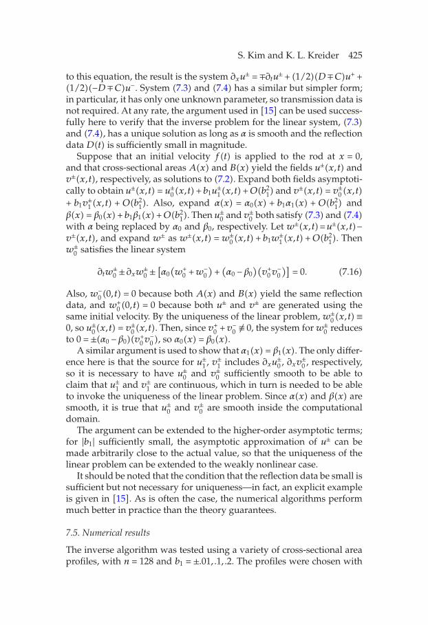
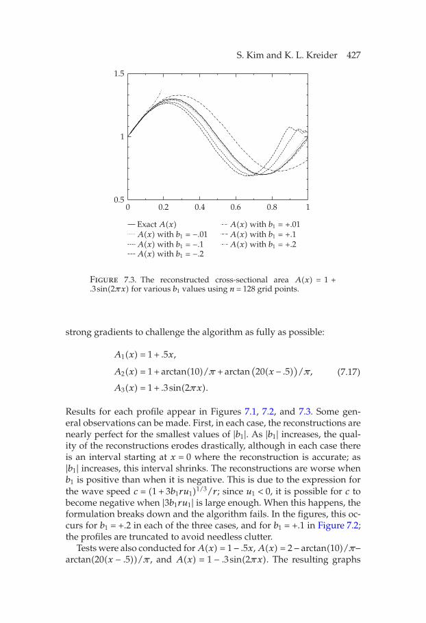
Figure 7.1. The reconstructed cross-sectional area A(x) = 1+ .5x forvarious b1 values using n = 128 grid points.

10.80.60.40.200.5

1

1.5

2

2.5

Exact A(x)A(x) using b1 = −.01A(x) using b1 = −.1A(x) using b1 = −.2

A(x) using b1 = +.01A(x) using b1 = +.1A(x) using b1 = +.2

Figure 7.2. The reconstructed cross-sectional area A(x) = 1 +arctan(10)/π + arctan(20(x − .5))/π for various b1 values using n =128 grid points.


10.80.60.40.200.5

1

1.5

Exact A(x)A(x) with b1 = −.01A(x) with b1 = −.1A(x) with b1 = −.2

A(x) with b1 = +.01A(x) with b1 = +.1A(x) with b1 = +.2

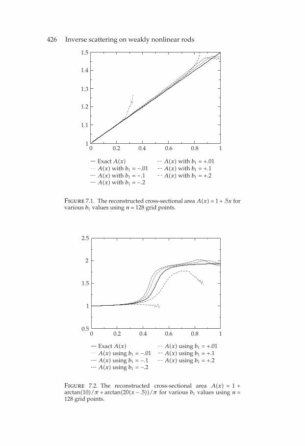
Figure 7.3. The reconstructed cross-sectional area A(x) = 1 +.3sin(2πx) for various b1 values using n = 128 grid points.

strong gradients to challenge the algorithm as fully as possible:

A1(x) = 1+ .5x,

A2(x) = 1+ arctan(10)/π + arctan(20(x − .5)

)/π,

A3(x) = 1+ .3sin(2πx).

(7.17)

Results for each profile appear in Figures 7.1, 7.2, and 7.3. Some gen-eral observations can be made. First, in each case, the reconstructions arenearly perfect for the smallest values of |b1|. As |b1| increases, the qual-ity of the reconstructions erodes drastically, although in each case thereis an interval starting at x = 0 where the reconstruction is accurate; as|b1| increases, this interval shrinks. The reconstructions are worse whenb1 is positive than when it is negative. This is due to the expression forthe wave speed c = (1 + 3b1ru1)1/3/r; since u1 < 0, it is possible for c tobecome negative when |3b1ru1| is large enough. When this happens, theformulation breaks down and the algorithm fails. In the figures, this oc-curs for b1 = +.2 in each of the three cases, and for b1 = +.1 in Figure 7.2;the profiles are truncated to avoid needless clutter.

Tests were also conducted for A(x) = 1− .5x, A(x) = 2− arctan(10)/π−arctan(20(x − .5))/π , and A(x) = 1 − .3sin(2πx). The resulting graphs


10.80.60.40.200.6

0.8

1

1.2

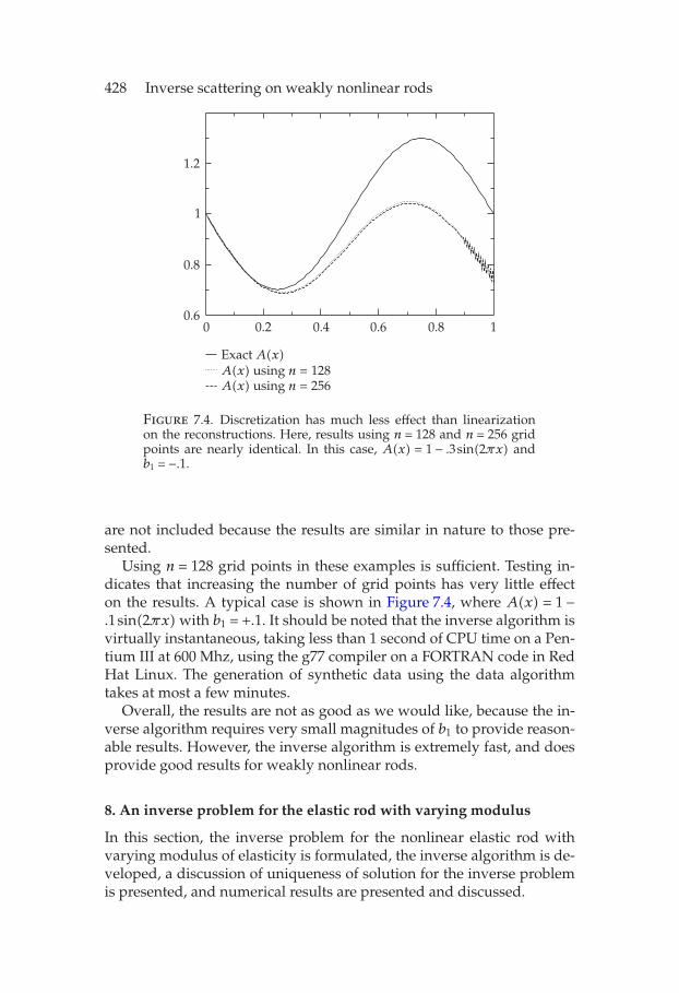
Exact A(x)A(x) using n = 128A(x) using n = 256

Figure 7.4. Discretization has much less effect than linearizationon the reconstructions. Here, results using n = 128 and n = 256 gridpoints are nearly identical. In this case, A(x) = 1 − .3sin(2πx) andb1 = −.1.

are not included because the results are similar in nature to those pre-sented.

Using n = 128 grid points in these examples is sufficient. Testing in-dicates that increasing the number of grid points has very little effecton the results. A typical case is shown in Figure 7.4, where A(x) = 1 −.1sin(2πx) with b1 = +.1. It should be noted that the inverse algorithm isvirtually instantaneous, taking less than 1 second of CPU time on a Pen-tium III at 600 Mhz, using the g77 compiler on a FORTRAN code in RedHat Linux. The generation of synthetic data using the data algorithmtakes at most a few minutes.

Overall, the results are not as good as we would like, because the in-verse algorithm requires very small magnitudes of b1 to provide reason-able results. However, the inverse algorithm is extremely fast, and doesprovide good results for weakly nonlinear rods.

8. An inverse problem for the elastic rod with varying modulus

In this section, the inverse problem for the nonlinear elastic rod withvarying modulus of elasticity is formulated, the inverse algorithm is de-veloped, a discussion of uniqueness of solution for the inverse problemis presented, and numerical results are presented and discussed.



For this problem, the stress-strain relation is again taken to be

σ = F(x,ε) = E(x)(ε + b1ε

2), (8.1)

where b1 1 and the scalings ρ = 1, A = 1 are used. The dynamic equa-tions take the form

∂t

(u+

u−

)=

(−cn 0

0 cn

)∂x

(u+

u−

)+

−12N

12N

, (8.2)

where, for this case,

N =1cτ

(∂xF − c∂xg

)=dE/dx

cτ

(ε + b1ε

2 − c(u+ +u−)

2E

). (8.3)

The nonlinear source term F, as well as the wave speeds, couple thetwo equations. The leading order asymptotic expansion of the dynamicequations yields

∂tu+0 +E(x)1/2∂xu

+0 = −dE/dx

4E(u+

0 +u−0

),

∂tu−0 −E(x)1/2∂xu

−0 =

dE/dx

4E(u−

0 +u−0

).

(8.4)

It is convenient to apply the travel time coordinate transformation

� =∫d

0E−1/2(x′)dx′, z =

1�

∫x

0E−1/2(x′)dx′, s =

t

�(8.5)

which converts (8.4) into the computational forms

∂sv+ + ∂zv

+ = − H ′

4H3/2

(v+ +v−),

∂sv− − ∂zv

− =H ′

4H3/2

(v+ +v−).

(8.6)

Here, H(z) = E(x(z)), H ′ = dH/dz, and v±(z,s) = u±(x,t).Again, the wave speed has been linearized and the equations remain

coupled. The dynamic equations may be solved using the method ofcharacteristics.



Consider the recovery of H(z) from reflection data v−(0, s) =D(s) with-out knowledge of b1. The reflection data is obtained by solving the directproblem, using the correct values of b1 and H(z) as inputs. Then, theleading order equations (8.6) are solved numerically to obtain the val-ues of H(zi) at each spatial grid point. Then the travel time transforma-tion is used to obtain the value of physical value of xi associated witheach computational value zi. As with the varying cross-sectional area,the method is appropriate only for very weakly nonlinear materials.

The inverse problem is specified as follows: the dynamic equations(8.6) are combined with boundary conditions

v+(0, s) =D(s)− f(s), v−(0, s) =D(s) (8.7)

and leading edge conditions

v+(z,z+) = −f(0)exp((H−1/2(z)− 1

)/2), (8.8)

v−(z,z+) = 0, (8.9)

where f(s) is the known applied velocity at the left boundary and D(s)is the reflection data, to form a well-posed problem. Equation (8.8) isobtained in the same manner as (7.6).

At this point, the inverse algorithm is the same as that for the varyingcross-sectional area, with one difference. The algorithm provides discretevalues of Hi at the points zi. These values must be converted to physicalcoordinates to obtain the desired E(xi) values. These values are obtainedby discretizing the travel time transformation equation and solving iter-atively for xi:

h = zi − zi−1 =1σ

∫xi

xi−1

E−1/2(x′)dx′

≈ 1σ

xi −xi−1

2(E−1/2i +E−1/2

i−1

)=

1σ

xi −xi−1

2(H−1/2

i +H−1/2i−1

).

(8.10)


Suppose that H ′(z)/4H3/2(z) is smooth, that |b1| is sufficiently small,and that the reflection data D(s) = u−(0, s) is sufficiently small in magni-tude. Then the inverse problem, to recover A(x) from the reflection data,has a unique solution.


10.501

1.1

Exact E(x)E(x) with b1 = −.1E(x) with b1 = −.1E(x) with b1 = −.2

E(x) with b1 = +.1E(x) with b1 = +.1E(x) with b1 = +.2

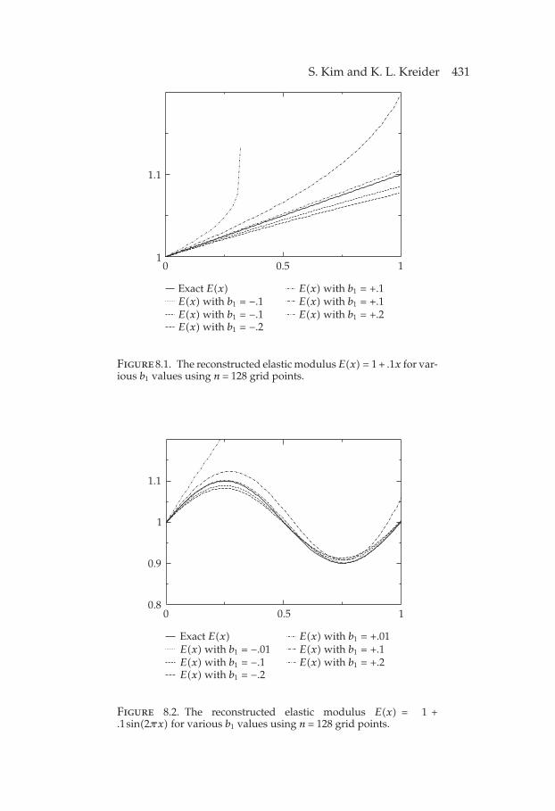
Figure 8.1. The reconstructed elastic modulus E(x) = 1+ .1x for var-ious b1 values using n = 128 grid points.

10.500.8

0.9

1

1.1

Exact E(x)E(x) with b1 = −.01E(x) with b1 = −.1E(x) with b1 = −.2

E(x) with b1 = +.01E(x) with b1 = +.1E(x) with b1 = +.2

Figure 8.2. The reconstructed elastic modulus E(x) = 1 +.1sin(2πx) for various b1 values using n = 128 grid points.


The proof follows the format used to show uniqueness for the varyingcross-sectional area problem in the previous section.


A number of numerical tests were performed to study this case. The fol-lowing modulus profiles were studied:

E1(x) = 1+ .1x, E2(x) = 1+ .1sin(2πx). (8.11)

The results are shown in Figures 8.1 and 8.2. The main observation tobe made here is that the inverse algorithm is much more sensitive tovariations in modulus than it is to variations in the cross-sectional area.This makes sense, because the modulus appears in the stress-strain re-lation and hence plays a more significant role in determining the natureof wave propagation through the rod. However, the results match qual-itatively with those for the varying cross-sectional area: small |b1| valueslead to good reconstructions, larger |b1| values lead to worse reconstruc-tions, and if b1 is large enough, the algorithm fails because the wavespeed becomes negative.

Tests were also conducted for E(x) = 1− .1x and E(x) = 1− .1sin(2πx)with results similar to those presented.

9. Conclusion

In this paper, elastic wave propagation in weakly nonlinear elastic rodsis considered in the time domain. The method of wave splitting is em-ployed to formulate a standard scattering problem, forming the mathe-matical basis for both direct and inverse problems. The focus here is ondeveloping algorithms for solving the inverse problem. An asymptoticapproach is used to linearize the dynamic equations. The goal is to de-termine the conditions for which this approach is reasonable, and to usethe insight gained here to develop more robust inverse algorithms.

For the homogeneous nonlinear rod, the asymptotic approach leads toan analytic expression for the transmitted field, which is used in a leastsquares sense to recover the nonlinear parameter b1. For the homoge-neous rod with varying cross section and the rod with varying modulusof elasticity, the method of characteristics is used to recover the respec-tive material parameter as a function of depth into the rod.

Numerical results indicate that although the inverse algorithms areextremely fast, the asymptotic approach yields good results only whenthe nonlinearity in the stress-strain relation is very weak. For even mod-erate nonlinearities, another approach is needed for solving inverseproblems.


Despite the limited usefulness of the algorithms presented here, thereare some valuable insights to be gained from this work. The elastic mod-ulus affects wave propagation much more strongly than does the cross-sectional area in nonlinear elastic rods, because of its appearance in thestress-strain relation. The results here indicate that it is reasonable to pur-sue a method that works in a global sense—these algorithms work wellnear the incident boundary, with results that gradually worsen deeperinto the rod, and with occasional sudden failures. An algorithm that doesnot use this “layer stripping” approach may work much better.

This paper is a first step in determining practical algorithms for solv-ing inverse problems on nonlinear rods in the time domain. Work is cur-rently underway to include higher-order asymptotic terms, to investi-gate the effects of noisy data on this method, and to consider other ap-proaches to solving such inverse problems. One such approach is theoptimization method presented in [8]. Although the context here is elas-ticity, the analysis and numerics work just as well in electromagneticsand acoustics.

Acknowledgment

The authors would like to thank the referees for making numerous sug-gestions that improved the presentation of the paper.

References

[1] I. Aberg, High-frequency switching and Kerr effect—nonlinear problems solvedwith nonstationary time domain techniques, J. Electro. Waves Applic. 12(1998), 85–90.

[2] J. Achenbach, Wave Propagation in Elastic Solids, North-Holland, Amsterdam,1973.

[3] W. F. Ames, Numerical Methods for Partial Differential Equations, 3rd ed., Com-puter Science and Scientific Computing, Academic Press, Massachusetts,1992.

[4] E. Ammicht, J. P. Corones, and R. J. Krueger, Direct and inverse scattering forviscoelastic media, J. Acoust. Soc. Amer. 81 (1987), no. 4, 827–834.

[5] D. V. J. Billger and P. D. Folkow, The imbedding equations for the Timoshenkobeam, J. Sound Vibration 209 (1998), no. 4, 609–634.

[6] T. J. Connolly and D. J. N. Wall, On some inverse problems for a nonlinear trans-port equation, Inverse Problems 13 (1997), no. 2, 283–295.

[7] J. Corones and A. Karlsson, Transient direct and inverse scattering for inhomo-geneous viscoelastic media: obliquely incident SH mode, Inverse Problems 4(1988), no. 3, 643–660.

[8] P. D. Folkow and K. Kreider, Direct and inverse problems on nonlinear rods,Math. Comput. Simulation 50 (1999), no. 5-6, 577–595.


[9] P. Fuks, G. Kristensson, and G. Larson, Permittivity profile reconstructions us-ing transient electromagnetic reflection data, Electromagnetic Waves PIER 17(J. A. Kong, ed.), EMW Publishing, Massachusetts, 1997, pp. 265–303.

[10] A. Gedroits and V. Krasilnikov, Finite-amplitude elastic waves in solids and de-viations from Hooke’s law, Soviet Phys. JETP 16 (1963), 1122–1126.

[11] M. A. Itskovitš, Generalization of the Achenbach-Chao model for waves in non-linear hereditary media, Internat. J. Non-Linear Mech. 31 (1996), 203–210.

[12] A. Karlsson, Inverse scattering for viscoelastic media using transmission data, In-verse Problems 3 (1987), 691–709.

[13] S. Kim, Asymptotic solutions of inverse scattering problems on weakly nonlinearelastic rods, Master’s thesis, The University of Akron, Ohio, 1999.

[14] G. Kristensson and R. J. Krueger, Direct and inverse scattering in the time do-main for a dissipative wave equation. I. Scattering operators, J. Math. Phys. 27(1986), no. 6, 1667–1682.

[15] , Direct and inverse scattering in the time domain for a dissipative waveequation. II. Simultaneous reconstruction of dissipation and phase velocity pro-files, J. Math. Phys. 27 (1986), no. 6, 1683–1693.

[16] G. Kristensson and D. J. N. Wall, Direct and inverse scattering for transient elec-tromagnetic waves in nonlinear media, Inverse Problems 14 (1998), no. 1,113–137.

[17] A. A. Lokshin and M. A. Itskovitš, A note concerning generalization of the Lan-dau method for waves in nonlinear hereditary media, Internat. J. Non-LinearMech. 23 (1988), no. 2, 125–129.

[18] A. A. Lokshin, M. A. Itskovitš, and V. E. Rok, An acoustical investigationmethod for a bar with nonlinear inclusions, J. Acoust. Soc. Amer. 89 (1991),no. 1, 98–100.

[19] A. A. Lokshin and E. A. Sagomonyan, Nonlinear Waves in Inhomogeneous andHereditary Media, Springer-Verlag, Berlin.

[20] K. R. McCall, Theoretical study of nonlinear elastic wave propagation, J. Geophys.Res. 99 (1994), 2591–2600.

[21] J. K. Na and M. A. Breazeale, Ultrasonic nonlinear properties of lead zicronate-titanate ceramics, J. Acoust. Soc. Amer. 95 (1994), no. 6, 3213–3221.

[22] U. Nigul, Asymptotic analyses of the pulse shape evolution and of the inverse prob-lem of acoustic evaluation in case of the nonlinear hereditary medium, Nonlin-ear Deformation Waves. Proceedings of the IUTAM Symposium, Tallinn,August 22–28, 1982, Springer-Verlag, Berlin, 1983, pp. 255–272.

[23] L. A. Ostrovsky, Wave processes in media with strong acoustic nonlinearity, J.Acoust. Soc. Amer. 90 (1991), no. 6, 3332–3337.

[24] Y. Rabotnov, Y. Suvorova, and A. Osokin, Deformation waves in nonlinearhereditary media, Nonlinear Deformation Waves. Proceedings of the IU-TAM Symposium, Tallinn, August 22–28, 1982, Springer-Verlag, Berlin,1983, pp. 157–170.

[25] D. Sjöberg, Reconstruction of nonlinear material properties for homogeneous,isotropic slabs using electromagnetic waves, Inverse Problems 15 (1999),no. 2, 431–444.

[26] J. A. TenCate, K. E. A. Van Den Abeele, T. J. Shankland, and P. A. Johnson,Laboratory study of linear and nonlinear elastic pulse propagation in sandstone,J. Acoust. Soc. Amer. 100 (1996), no. 3, 1383–1391.


Shinuk Kim: Department of Theoretical and Applied Mathematics, The Univer-sity of Akron, Akron, OH 44325-4002, USA

E-mail address: [email protected]

Kevin L. Kreider: Department of Theoretical and Applied Mathematics, TheUniversity of Akron, Akron, OH 44325-4002, USA

E-mail address: [email protected]

mailto:[email protected]

mailto:[email protected]

Documents

An asymptotic approach to inverse scattering problems on ... fileAn asymptotic approach to inverse scattering problems on