Inverse Problems 4 (1988) 4355.147. Printed i n the U K

Three-dimensional inverse scattering for the wave equation: weak scattering approximations with error estimates

Margaret Cheneyi and James H Rose4 ?Department of Mathematics, Duke University, Durham, NC 27706, USA $Amc\ Laboratory USDOE, Iowa State University, Ames, IA 50011. USA

Received 6 April 1987, in final form 24 July 1987

Abstract. The reduced wave equation for an inhomogeneous medium ib considered. Low- and intermediate-frequency scattering data are assumed to be known exactly for one direction of incidence and all directions of scatter. From these data, the index of refraction in the medium is recovered approximately in two different ways. Moreover, explicit error estimates for the two methods are derived.

1. Introduction

The inverse scattering problem for wave propagation in an inhomogeneous medium arises in a variety of fields. For example, this problem must be solved in ultrasound imaging of biological tissue, non-destructive inspection of materials and seismic prospecting. Unfortunately, at present, there are no exact methods of solving this problem that are also numerically tractable. Instead, researchers must resort either to iterative schemes that are not well understood, or to approximations of various sorts.

The approximations most often used are those that assume that the scattering is weak in some sense. This kind of assumption has been used by a very large number of authors to derive various inversion methods. References to this work can be found in [l] for acoustics, [2] for elastodynamics and [3] for electrodynamics. A recent publication with references is that of Porter [4]. Generally these inversion methods carry with them no error estimates or precise conditions under which one can be sure of obtaining good answers.

As we will see, it is possible to f i l l this gap in a number of cases. In this paper, two approximate (weak scattering) inversion methods are rederived and error estimates are obtained for them. In both methods, we will assume that the frequency of the probing wave multiplied by the perturbation in the medium is small in a certain sense. This will be our weak scattering assumption. We will also assume that scattering data are known at low frequencies for a single direction of the incident wave and for all scattered directions. We will see that what is reconstructed is, up to a certain error, a blurred version of the perturbation in the medium. We will obtain explicit blurring functions and explicit error estimates.

The plan of the paper is as follows. In D 2 we set up the problem and show how to recover the perturbation from certain approximations to the data. In B 3 we derive the two approximate inversion methods together with specific blurring functions and error

0266-561 1/88/02O435+ 13 $02.50 @ 1988 IOP Publishing Ltd 435

436 M Cheney and J H Rose

estimates. The main results are given in theorems 1 and 2. In 9 4 we show how these approximate methods are related to’ an inverse scattering integral equation recently derived [5-71.

2. Background

We consider the equation

(a’+ k2n’(x) )q(k , x) = 0 (2.1) where x E R’,V’ denotes the Laplacian and k is a real scalar. The index of refraction is described by a scalar function n(x) which is assumed to be one for large 1x1. Scattering solutions of (2.1) can be defined by means of the Lippmann-Schwinger equation

exp(ik’x-yl) k’(1 -n2 (y ) )q (k , e, y ) dy - 4+ - yl

q ( k , e, x) = exp(ike - x) + where e is a unit vector denoting the direction of the incident plane wave. A solution I+ of (2.2) will sometimes be referred to as a ‘wave field’ and we will write V ( x ) = 1 - n2(x). We note that this sign convention for V is the opposite of that in [ 5 ] .

We will need the following quantity, which is called the scattering amplitude:

(2.3)

It can be measured in either of two ways. The first way is to measure q for very large 1x1 (i.e. use far-field data). For large 1x1,

y(k. e , x) = exp(ike x) + A ( k , i, e) exp(ik/x/)lx$’ + o(ixl-’) (2.4) where R denotes xilxl. Ikebe ([8], Lemma 3.2) has given conditions on V under which (2.4) holds. The scattering amplitude can also be measured from near-field data using the formula [9]

A(k. e , e’) = - (4x)-’

where aQ is any smooth surface enclosing the support of V and Y denotes the outward unit normal to 82.

The inverse scattering problem is to recover V (which we will sometimes call the ‘potential’) from the data A . This problem will be considered under conditions in which the perturbation k2V is small in some sense. Such conditions we call ‘weak scattering conditions’.

Under weak scattering conditions, the solution y ( k , e, x) is very nearly equal to the incident wave exp(ike-x). In this case the scattering amplitude is very nearly equal to its Born approximation, which we denote by AB:

exp( - ike x ) [ v C I + ( ~ , e’. x) + ike vy/(k, e’ , x)] dx J dL1

(2 .5 )

k’ 4x

- _ _ - V [ k ( e - e ‘ ) ]

3 0 inverse scattering for the wuue equation 437

where the hat denotes the Fourier transform. We can see from (2.5) that the inverse scattering problem under weak scattering

conditions will be closely related to the problem of recovering a function from its Fourier transform. Some Fourier inversion formulae are therefore reviewed next. In what follows, the notation S2 denotes the unit sphere in R3.

Lemma 1. Let VE L2(R’) and let pdenote its Fourier transform. Then for any e E S’, V can be recovered from p by means of the following formula:

Proof, We write the usual inversion formula in spherical coordinates:

V(x) = --& i: I V(so) exp(isw x) dw s’ ds. ( 2 4 $1

We split the angular integral into two parts, the parts corresponding to e * w > 0 and e w<O, respectively. In the part corresponding to e * w <0, we make the change of variables 0- - w and s-+ -s. QED

We also recall from reference [lo] a low-pass filtered Fourier inversion formula. To state this formula, we define for any k>O

where xk denotes the function that is one inside the ball of radius 2k and zero outside.

Lemma 2. [lo] Let VE L2(R3) and let p denote its Fourier transform. Then for any k>O,

VLll(k, x) = (2x)-‘k’ V [ k ( e - e’)] exp[ik(e - e’) x]le - e’l de de’.

Next, we use (2 .5) to write (2.6) and (2.8) in terms of the Born approximation.

Proposition 1. [ll] Let VE L*([W”). Then V can be recovered from the Born approxi- mation by the following formula:

V ( x ) = - & I:, 1 A,(k, e, e’) exp[ik(e - e’) x] le - e’I2 de’ dk. 52

Proof. We use Lemma 1 together with the change of variables w = (e - e’)/le - e’l, dw = - (2le - e’l)-’de’, s = k/e - e’l. We note that as e’ varies over S’, w varies over the half of S’ with e * w > 0. QED

438

Proposition 2. [lo] Let VE L2(R3) and let k be positive. Then

M Cheney and J H Rose

VLP(k, x) = - - AB(k , e, e’) exp[ik(e - e’) . x]le - e’l de de’. (2. lo)

Having seen from (2.9) and (2.10) that the Born approximation is useful for inverse scattering, we now consider how well the Born approximation AB approxi- mates the true scattering amplitude A . As mentioned above (2.5), A is close to AB under weak scattering conditions. In order to express this precisely, we will need several norms. First, 1 1 . I / R is [12]

We note that the Rollnik norm of V is finite if V is in L’(R3) and I,’@’) [12]. We will denote by 1 1 * / I l and 11 I / * the norms on L’ and L’, respectively.

Proposition 3. Let V E L’ n L’, and suppose that lkl< k,, = (4n /~~V~~R)”2 . Then

Proof. We use (2.3) and (2.5) to compute the left-hand side of (2.11):

exp( -ike .x)V(x)[q(k, e’,x)-exp(ike’ -x)]

To (2.12) we apply the Schwarz inequality, obtaining

(2.11)

(2.12)

(2.13)

We use (2.2) to estimate the right-hand side of (2.13). We multiply (2.2) by 1V(x)l”’, obtaining the equation

1 VI”+) = E + Kk( 1vI 1”q) (2.14)

where

E(k, e, x) = /V(x)I”’ exp(ike e x ) (2.15)

and

3 0 inverse scattering for the wave equation 339

We can easily compute the operator norm /iKkli with the help of the Hilbert-Schmidt norm i i ~ i i ~ ~ 1131:

For lkl< k,,, I/Kkl/ is less than one, so that (2.14) can be solved by iteration. We obtain

(2.17)

We use this again in (2.14), obtaining

We use (2.18) in (2.13) to obtain (2.11). QED

We note that proposition 3 gives us useful information when k’V is small. This would not be the case if the right-hand side of (2.11) were merely of order k’Vfor k2V small, because both A and A B are themselves of order k2V. However, (2.11) tells us that A and A B are closer to each other than they are to zero.

3. Weak scattering methods 1 and 2

We now consider the inverse scattering problem. In this section we will present two inversion methods. The fact that there are two inversion methods (and probably many more) arises because A is a function of five variables whereas V is a function of only three. These inversion methods are good in the sense that if V is weak enough, the reconstruction is close to being exact. The precise sense in which this is true will be made clear by the estimates.

First we consider an inversion method based on proposition 1. Proposition 1 is only useful under weak scattering conditions (k2V small), but the inversion formula (2.9) involves an integral over all k. We must therefore modify (2.9). To restrict formula (2.9) to sufficiently low frequencies, we introduce a cut-off function a(k ) which is zero for lkl larger than some kO<(4;2/11VllR)”’. When we insert a(k) into formula (2.9), we must replace V by a blurred potential which we denote by VI . Specifically,

V , ( x , e ) = - $ l:z a(k) 1 AB(k, e, e’) exp[ik(e - e’) - x] le - e’l’ de’ dk. (3.1) \2

440 M Cheney and J H Rose

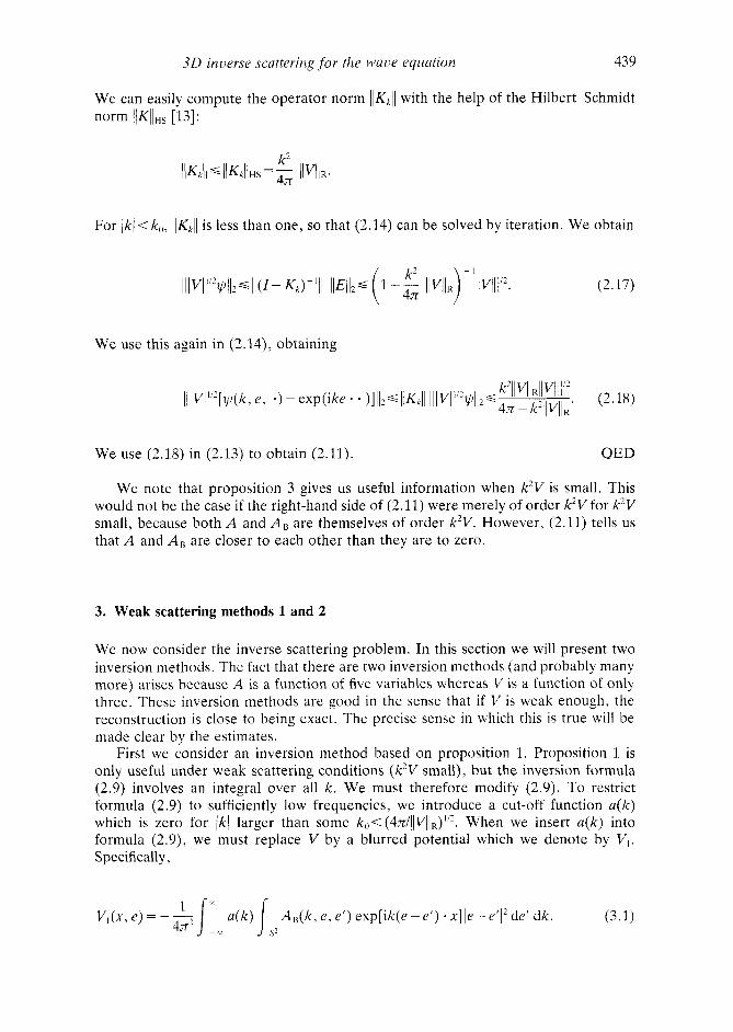
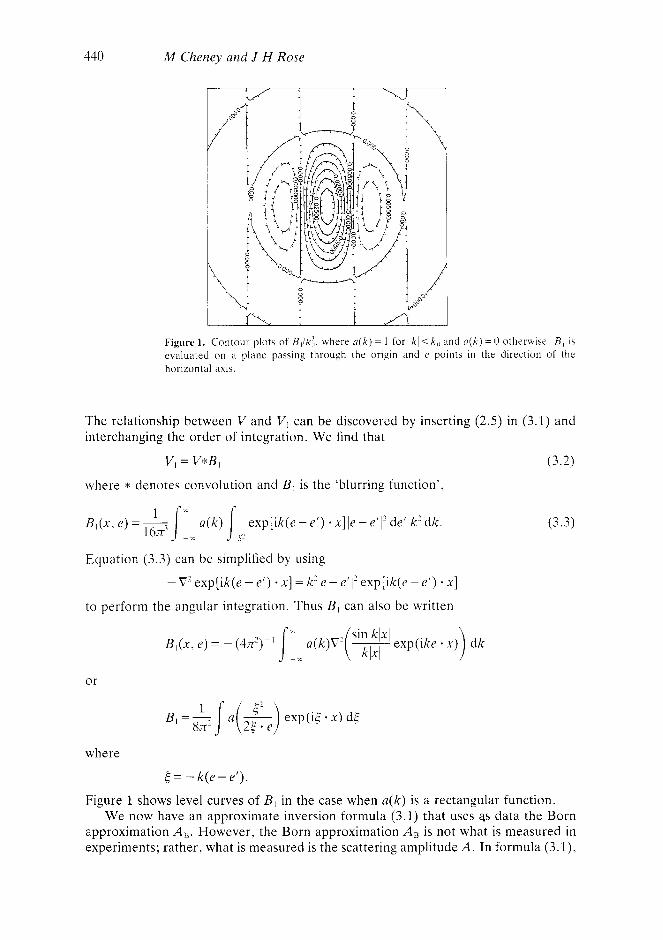
Figure 1 . Contour plots of Z?,/k,;. where u ( k ) = 1 for lkl< k , , and a ( k ) = 0 otherwise. R , is evaluated on a plane passing through the origin and e points in the direction of the horizontal axis.

The relationship between V and VI can be discovered by inserting (2.5) in (3.1) and interchanging the order of integration. We find that

V , = V*B, (3 .2) where :P denotes convolution and B , is the 'blurring function',

(3 .3)

Equation (3.3) can be simplified by using

- C' exp[ik(e - e ' ) x] = k'le - e ' /? exp[ik(e - e ' ) x] to perform the angular integration. Thus B , can also be written

or

where

c = - k ( e - e ' ) .

Figure 1 shows level curves of B , in the case when a ( k ) is a rectangular function. We now have an approximate inversion formula (3.1) that uses 3s data the Born

approximation AB, However, the Born approximation AB is not what is measured in experiments; rather, what is measured is the scattering amplitude A . In formula (3.1),

30 inverse scattering for the wave equation 44 1

we therefore replace A B by A . In doing so, we introduce an error, which we denote by R A :

x exp [ik(e - e’) - x] le - e’/’ de‘ dk + R A ( x , e) . (3.4)

Theorem I . Let V E L ’ n L2 and let a(k) be a real-valued function that is zero for Ikl? kO. Then (3.4) holds, with

Proof. We compute RA:

x exp[ik(e - e’) x]le - e‘\’ de’ dk 1 . (3.6)

In (3.6) we use proposition 3. We then merely compute J& - e’/’ de‘ = 8x to obtain (3.5). QED

We note that our reconstruction formula (3.4) requires only part of the infor- mation contained in A ( k , e, e‘). In particular, A need be known only for one incident direction. all scattered directions and small frequencies.

Next we consider an inversion method (10) based on proposition 2. In (2.10), we replace A B by A . In doing so, we introduce an error, which we denote by R,,,:

(3.7) V , , , ( k , ~ ) = ~ [ ~ j - k A(k,e,e’)exp[ik(e-e’) * ~ ] l e - e ’ I d e d e ’ + R , ~ ( k , x ) .

\>

Theorem 2. Let V E L ’ n L2 and suppose that O<k<k0=(4~/1~~/llK)”*. Then (3.7) holds, with

Proof. We compute RLp:

x exp[ik(e - e’) x]je - e’l de de‘ . (3.9)

442 M Cheney and J H Rose

In (3.9) we use proposition 3 and the fact that

to obtain (3.8). QED The reconstruction VLp can also be written as a convolution. This becomes evident

when we write in terms of V in (2.7). Then, after an interchange of the order of integration, (2.7) is

VLp = B2* V where

(3.10)

B,(k, x) = (2n)-3 xk(t) exp(i6 x) d< i As noted in [lo], the reconstruction (3.7) takes place at a fixed frequency. At this

fixed value of k , the scattering amplitude is a function of four variables. The reconstruction (3.7) is therefore using redundant information.

4. Connections with an inverse scattering equation

The preceding methods of recovering the potential from the low- and intermediate- frequency scattering amplitude can be obtained from the equation [5-71

where q’ = y is defined by (2.2) and y - is defined by

y - ( k , e, x ) = ~ + ( - k , -e, x ) .

The function y - satisfies

exp( - iklx - y i ) k2V(y )q - (k , e , y ) dy. i - 4n/x - yI q - ( k , e, x) = exp(ike x) + (4.3)

Equation (4.1) holds under the conditions stated in theorem 2 below. It is natural to investigate (4.1) in the context of weak scattering because (4.1) lies

at the heart of a number of exact inverse scattering methods. Equation (4.1) was used by Newton in 1979 to solve the inverse scattering problem for the Schrodinger

3 0 inverse scattering for the wave equatiorz 443

equation in three dimensions (see [14] and references therein). Equation (4.1) is also useful [5-71 in attacking the inverse scattering problem for the variable velocity wave equation (2.1).

However, (4.1) as it stands is hard to use, because it has infinitely many solutions. These arise because x appears only as a parameter in the solution. Thus for each x , the wave field W(k, * , x) gives a different solution of (4.1). Consequently it is difficult to see in general how to solve for the velocity potential V using this equation. Below, we will show that in the weak scattering limit (4.1) in fact can be used to derive the approximate reconstruction methods of the previous section.

We will use the weak scattering assumption to simplify both sides of (4.1). On the left-hand side, we use (2.2) and (4.3), obtaining

y ~ + ( k , e , x) - y - ( k , e , x)

where

x k ’ V ( z ) q - ( k . e, z ) dz dy.

We use the Schwarz inequality several times in estimating R I :

In (4.6) we use (2.17), obtaining for k < k , , = (4n/)lIllR)”*

(4.5)

444 M Cheney and J H Rose

Next we consider the right-hand side of (4.1). For y - we substitute the right-hand side of (4.3), obtaining

where

We use (4.3) and the Schwarz inequality to estimate R1:

In (4.10) we use (2.17) and carry out the e‘ integral:

We now see that we can simplify (4.1) with the help of (4.4) and (4.8):

exp(ik1x - y i ) - exp( - ikjx - yj) k’V(y) exp(ike y ) d y - 4x1~ - y /

A ( k , e’, e) exp(ike‘ - x) de‘ + (R? - R , ) ( k , e , x). 2,2

(4.11)

(4.12)

To obtain a convolution on the left-hand side of (4.12), we multiply the entire equation by 2ink-? exp( - ike - x), Equation (4.12) then becomes

(B+V)(k, e , x) = - - A ( k , e’ , e) exp[ - ik(e - e’) x] de’ + R, (k , e, x) (4.13) k ‘i 5 2

where

sinklxl B 3 ( k , e, x) =- exp( - ike - x) 1x1

and

R;(k , e, x) = 2irck-’exp( - ike x)(R2 - R , ) ( k , e , x).

(4.14)

(4.15)

We have proved the following theorem.

3 0 inverse scattering for the wave equation 445

Theorem 3. Let V E L ’ n L’ with V(x)=O(lxl-”-‘) for some E > O and let k < (4n/11qlR)”’. Then (4.13) holds, and R1 satisfies

(4.16)

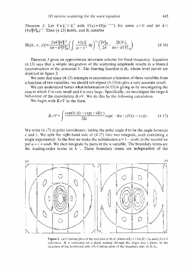
Theorem 3 gives an approximate inversion scheme for fixed frequency. Equation (4.13) says that a simple integration of the scattering amplitude results in a blurred reconstruction of the potential V. The blurring function is B1, whose level curves are depicted in figure 2.

We note that since (4.13) attempts to reconstruct a function of three variables from a function of two variables, we should not expect (4.13) to give a very accurate result.

We can understand better what information (4.13) is giving us by investigating the case in which Vis very small and k is very large. Specifically, we investigate the large-k behaviour of the convolution B,*V. We do this by the following calculation.

We begin with B p V in the form

exp(iklz1) - exp( - ik/z/) exp( - ike z )V(x - z ) dz. (4.17) i 2ilz/

B3*V=

We write (4.17) in polar coordinates, taking the polar angle 8 to be the angle between e and z . We split the right-hand side of (4.17) into two integrals, each containing a single exponential. In the first we make the substitution U = 1 - cos8; in the second we put U = 1 + cose. We then integrate by parts in the U variable. The boundary terms are the leading-order terms in k-I. These boundary terms are independent of the

Figure 2. (a) Contour plots of the real part of B , / k , , where a ( k ) = 1 for I k l i k, , and u ( k ) = 0 otherwise. B , is evaluated on a plane passing through the origin and e piontr in the direction of the horizontal axis. ( b ) Contour plots of the imaginary part of B3/k , , .

446 M Cheney and J H Rose

azimuthal angle, so the azimuthal integration can be carried out in the leading-order terms. At this stage we have

V(x+se)exp(2iks) ds+o(k-l) . (4.18)

However, if Vis absolutely integrable on each line, the second term on the right-hand side of (4.18) is also o ( k - l ) . Thus we have

B3*V( k . e, x) = - V(x + se) ds + o( k - I ) . (4.19)

We see from (4.19) that in the large-k, small-V limit, B3*V is a line integral of V. Thus we expect that for low and intermediate values of k , B,*V is a blurred version of a line integral of V.

j',

Together, equations (4.19) and (4.13) tell us

V(x+se) ds= -xjy' A ( k , e ' , e) exp[ik(e'-e) e x ] de '+e r ro r . (4.20)

We can use (4.20) to obtain the inversion formula of (3.7). T o do this, we use the following formula to reconstruct V from its line integrals [15, 161:

V(x) = (2n) - j j,s2i lq/exP[-iq.(x-y)l VO:+se)dsdy dedq. (4.21)

Equation (4.21) can be verified by first substituting for y the variable z = y +se, then doing the s integral followed by the e integral. The e integral is

L 1 s2

J,.? d(e 4 ) de = 2 4 d .

Verification of (4.21) is then completed with the help of the Fourier inversion formula.

W e now use (4.20) in the right-hand side of (4.21). In the resulting expression, we carry out the y integral. A t this stage we have

x B[q + (e' - e ) k ] dq de de' + error. (4.22)

In (4.22), we carry out the q integral, make the substitutions e- - e and e'+ -e'. and use the reciprocity relation A ( k , - e ' , -e) = A ( k , e, e') to obtain (3.7). This calcula- tion allows us to see the connection between (3.7) and (4.13).

W e can also connect (4.13) to (3.4) as follows. First we rewrite B? as

(see the calculation below (3.3)). Then to both sides of (4.13) we apply the operator (2n'i)-'e - 0. O n each side, the e . 0 operates on exp[ - ik(e - e') * x], bringing down a

3 0 inverse scatteririg for the wave equation 447

factor of - ike - (e - e’) = - ikle - e’1’12. The resulting equation can be transformed into (3.4) by multiplying by (4n’)-’a(k) and integrating over all k . From this derivation of (3.4), however, it is more difficult to estimate the error term.

Acknowledgments

This research was partially supported by ONR grants #N000-14-85-K-0224 and N000-14-83-KO038. This work was begun while MC was visiting the Applied Mathematical Sciences group at Ames Laboratory. She gratefully acknowledges their hospitality.

References

[ 11 Esrnersoy C , Oristaglio M L and Levy B C 1985 Multiditnensional Born velocity inversion: Single wideband point source J . Acou~t . Soc. Am. 78 1052-7

121 Kogan V G and Rose J H 1Y85 Limited aperture effects on ultrasonic image reconstruction J . Acoust. Soc. Am. 77 1312-51

131 Boerner W-M 1980 Polarization utilization in electromagnetic inverse scattering Inoer.re Scattering Prohlems in Optics cd. H P Bates (New York: Springer)

[1] Porter R P 1986 Scattering wave inversion f o r arbitrary receiver geometry J . Acoust. Soc. Am. 80 122(L7

[SI Rose J H. Chcney M and DeFacio B 19x5 Three-ditncnsional inverse scattering: Plasma and variable telocity wave equations J . Mufh. Phys. 26 2803-13

161 Cheney M , Rosc J H and DeFacio B 1987 A fundamental integral equation o f scattering theory S I A M J . iMut/ i . Anal. i n press

[7] Rose J H. Cheney M and DeFacio B 1986 Determination of the wavefield from scattering data Phy.r. Reo. Let t . 57 783-6

[ X I lkebe T 1960 Eigenfunction expansions associated with the Schrcidinger operators and their appli- cations to scattering theory Arch. Rar. Mech. Arid. 5 1-34

191 Devaney A J and Beylkin G 1984 Diffraction tomography using arbitrary transmitter and receiver surfaces Ultrusonic Imugirig 6 181-93

[ I O ] Devaney A J 1982 Inversion fortnula for inverse scattering within the Born approximation Opr. Lert . 7 I 11-2

[ 1 1 I Langenbcrg K J and Schmitz V 1985 Generalized tomography as a unified approach to linear invcrse scattering Acousticul I m a g i n g vol. 14 ed. A J Berkhout et al (New York: Plenum)

[ 121 Simon B 1971 Q~4~1~trim Mechtrriics f o r Nurniltoniuri.s Defined us Quadrtrtic F o r m (Princeton. N J : Princeton University Press)

[ 131 Reed M and Simon B 1972 Meikods of Mocierrr MLrthernaticul Physics I: Fur7ctio,iul Ariulysis ( K e a York: Academic)

[ 141 Newton R G 1983 The Marchenko and Gcl’fand-Levitan methods in the inverse scattering problem in one and three dimensions Proc. Cotif: 017 Inoerse Scutteririg: Theory und Applicutiori ed. J B Bednar et U / (Philadelphia: SIAM)

[ 151 Smith K T 1984 Inversion 01 the x-ray transform Proc. SIAM-AMS Conf: Inuertr Problems vol. 14 cd. 11 W McLaughlin (Providcncc. RI: AMS)

[ lh] Smith K T and Keinert F 1985 Mathematical foundations of computed tomography Appl. Opt. 24 395(&7