Embed Size (px)
Citation preview

An inverse random source scattering problem in inhomogeneous media
This article has been downloaded from IOPscience. Please scroll down to see the full text article.
2011 Inverse Problems 27 035004
(http://iopscience.iop.org/0266-5611/27/3/035004)
Download details:
IP Address: 128.211.160.40
The article was downloaded on 23/02/2012 at 19:48
Please note that terms and conditions apply.
View the table of contents for this issue, or go to the journal homepage for more
Home Search Collections Journals About Contact us My IOPscience

IOP PUBLISHING INVERSE PROBLEMS
Inverse Problems 27 (2011) 035004 (22pp) doi:10.1088/0266-5611/27/3/035004
An inverse random source scattering problem ininhomogeneous media
Peijun Li
Department of Mathematics, Purdue University, West Lafayette, IN 47907, USA
E-mail: [email protected]
Received 27 August 2010, in final form 16 December 2010Published 4 February 2011Online at stacks.iop.org/IP/27/035004
AbstractConsider the scattering problem for the one-dimensional stochastic Helmholtzequation in a slab of an inhomogeneous medium, where the source function isdriven by the Wiener process. To determine the random wave field, the directproblem is equivalently formulated as a two-point stochastic boundary valueproblem. This problem is shown to have pathwise existence and uniquenessof a solution. Furthermore, the solution is explicitly deduced with an integralrepresentation by solving the two-point boundary value problem. Since thesource and hence the radiated field are stochastic, the inverse problem is toreconstruct the statistical structure, such as the mean and the variance, of thesource function from physically realizable measurements of the radiated fieldon the boundary point. Based on the constructed solution for the direct problem,integral equations are derived for the reconstruction formulas, which connectthe mean and the variance of the random source to those of the measured field.Numerical examples are presented to demonstrate the validity and effectivenessof the proposed method.
(Some figures in this article are in colour only in the electronic version)
1. Introduction
The inverse source scattering problem for wave propagation is largely motivated by medicalapplications in which it is desirable to use the measurements of electric or magnetic fieldon the surface of the human body, such as the head, to infer the source currents inside thebody, such as the brain, that produced these measured data. It has been considered as a basictool for the solution of reflection tomography, diffusion-based optical tomography, and morerecently fluorescence microscopy [29], where the fluorescence in the specimen, such as greenfluorescent protein, gives rise to emitted light which is focused to the detector by the sameobjective that is used for the excitation. In addition, the inverse source problem has attractedmuch research in the antenna community [12]. A variety of antenna-embedding materials
0266-5611/11/035004+22$33.00 © 2011 IOP Publishing Ltd Printed in the UK & the USA 1
Inverse Problems 27 (2011) 035004 P Li
or substrates, including plasmas, non-magnetic dielectrics, magneto-dielectrics, and, morerecently, double negative meta-materials are of interest.
The problem has been extensively investigated and there is much work on the scalarand the full vector electromagnetic inverse source problems in the free space as well as innonhomogeneous background media, see e.g. Albanese and Monk [1], Ammari et al [2], Ellerand Valdivia [14], Marengo et al [23], and references cited therein. It is also known thatthe inverse source problem does not have a unique solution due to the possible existence ofnonradiating sources, see e.g. Bleistein and Cohen [8], Devaney and Sherman [13], and Haueret al [17]. In order to obtain a unique solution, it is necessary to give additional constraintsthat the source must satisfy. A typical choice of the constraint is to take the minimum energysolution, which represents the pseudo-inverse solution for the inverse source problem, seee.g. Marengo and Devaney [22]. See also Bao et al [7] for a multi-frequency inverse sourceproblem in which the uniqueness is shown and some stability estimates are established fromthe radiated fields outside the source volume for a set of frequencies. A complete account ofthe general theory of inverse scattering problems may be found in Colton and Kress [10].
In this paper, we study the inverse random source scattering problem for the one-dimensional Helmholtz equation in a slab of the inhomogeneous medium, which is toreconstruct the statistical characteristics of the random source function. Since the source, andhence the radiated field, are modeled by random processes, the governing Helmholtz equationis considered as a stochastic differential equation instead of its deterministic counterpart.
Stochastic inverse problems refer to inverse problems that involve uncertainties andrandomness. Compared to classical inverse problems, stochastic inverse problems havesubstantially more difficulties on top of the existing hurdles, mainly due to the involvedrandomness and uncertainties. For instance, unlike the deterministic nature of solutions forclassical inverse problems, the solutions for a stochastic inverse problem are random functions.Therefore, it is less meaningful to find a solution for a particular realization of randomness.On the contrary, the statistics, such as mean and variance, of the solutions are more interesting.We refer to [4, 15, 16, 19, 27] for closely related imaging and wave propagation problems inrandom media, where the medium properties are modeled as random functions.
In the context of the inverse random source scattering problem, the goal is to deducethe statistical structure, such as the mean and the standard deviation or the variance of thesource function, from physically realizable measurements of the radiated fields, such as themeasurements taken on the boundaries. Although the deterministic counterpart has beenextensively investigated from both mathematical and numerical viewpoints, little is known forthe stochastic case, especially its computational aspect. A uniqueness result can be found inDevaney [11], where it is shown that the auto-correlation function of the random source isuniquely determined everywhere outside the source region by the auto-correlation function ofthe radiated field. Recently, a novel and efficient Wiener chaos expansion-based techniquehas been developed for modeling and simulation of spatially incoherent sources in photoniccrystals by Badieirostami et al [3]. See Bao et al [5] for a related inverse medium scatteringproblem with a stochastic source. One may consult Kaipio and Somersalo [20] for statisticalinversion theory for general random inverse problems.
This paper is an extension of the work [6], which considered the inverse random sourcescattering problem for the one-dimensional Helmholtz equation in a homogeneous backgroundmedium. For the homogeneous medium case, the solution for the direct problem is able to beanalytically constructed by using the integrated solution method. Explicit inversion formulascan also be derived to connect the mean and the variance of the random source function to theFourier transform of the measurements, which are implemented by the fast Fourier transform.Since explicit solutions will not be available any more for the inhomogeneous medium
2
Inverse Problems 27 (2011) 035004 P Li
case, the extension will be nontrivial and so the difference will be obvious from the workin [6].
The random source function, representing the electric current density, is assumed to havea compact support contained in a finite interval. The problem is modeled with an outgoingwave condition imposed on the lateral end points of the finite interval, which reduces themodel to a second-order stochastic two-point boundary value problem. This model problemis converted into an equivalent first-order stochastic two-point boundary value problem, andis shown to have a unique pathwise solution. By using the fundamental matrix, an integralequation is constructed for the solution of the direct problem. By studying the expectation andvariance of the integral equation, inversion formulas are deduced to reconstruct the mean andvariance of the random source function. Numerical examples are included to demonstrate thevalidity and effectiveness of the proposed method.
The paper is organized as follows. In section 2, we present the model problem andformulate it as a first-order two-point stochastic boundary value problem. The existence anduniqueness of the direct problem are established, and the solution is derived based on thefundamental matrix. We derive four integral equations, which build the construction formulasfor the mean and the variance of the source function. In section 3, we discuss numericalimplementation of the method and present three numerical examples to demonstrate thevalidity and effectiveness of the proposed approach. We conclude this paper with generalremarks and directions for future research in section 4.
2. Inverse random source problem
In this section, we introduce a mathematical model for the inverse random source scatteringproblem. The model problem is first converted into a stochastic two-point boundaryvalue problem. A theoretical framework for the direct model problem is established andreconstruction formulas are deduced for the solution of the inverse problem.
2.1. The model problem
Let u(x) be the time-harmonic wave field at location x with the time factor e−iωt omittedand assume that the slab occupies the interval [0, 1]. Then the wave field u satisfies theone-dimensional Helmholtz equation
u′′(x, ω) + ω2(1 + q(x))u(x, ω) = f (x), (2.1)
where the derivative is taken with respect to the spatial variable x, the magnetic permeabilityand the electric permittivity of the vacuum are assumed to be the unity for simplicity, ω > 0 isthe angular frequency, q > 0 implies the relative electric permittivity of the inhomogeneousmedium and has a compact support in the interval [0, 1], and f , representing the electriccurrent density, is a stochastic source function, which is assumed to have the form
f (x) = g(x) + h(x)W ′x.
Here g and h are the deterministic functions with compact supports contained in the intervalof the slab [0, 1], Wx is a one-dimensional spatial Wiener process, and W ′
x is its stochasticdifferential in the Ito sense which is commonly used as a model for the white noise, i.e. aspatial Gaussian random field. Throughout the paper, we assume that f, g, and h are thebounded functions in [0, 1], i.e. f, g, h ∈ L∞[0, 1]. Following from the standard stochastictheory on the white noise, we have
E[f (x)] = g(x) and V[f (x)] = h2(x),
3
Inverse Problems 27 (2011) 035004 P Li
where E and V are the expectation and variance operators, respectively. Thus g stands for themean value of the random source function and h characterizes the size of the fluctuation forthe random source. Obviously, due to the random nature of the source function, the solutionu, the radiate field, is also a random function. Typical boundary conditions imposed on u arethe so-called outgoing radiation boundary conditions, which are equivalent to the boundaryconditions at two lateral end points of the interval [0, 1]:
u′(0, ω) + iωu(0, ω) = 0 and u′(1, ω) − iωu(1, ω) = 0. (2.2)
Remark 2.1. The Wiener process is one of the two fundamental examples (the Poissonprocess is the simpler of the two) in the theory of continuous stochastic processes. Althoughwe only consider Gaussian random field driven by the Wiener process in this paper, the strategycan be extended to other types of randomness in the source function with minor modifications.For the completeness of the paper, some preliminaries, including the Wiener process andstochastic Ito integral, are briefly presented in the appendix.
There are usually two types of problems posed for the above equations. Given themean g and the standard deviation h of the random source function f , the direct problem is todetermine the random wave field u. On the contrary, the inverse source problem is to determinethe mean value g and the standard deviation h or the variance h2 of the random source from theboundary measurements of the random wave field u(0, ω), which is available for a sequenceof angular frequencies ω. Our goal is to investigate both the direct and inverse problems,and particularly propose a novel and efficient numerical algorithm to solve the inverse sourceproblem. Although we use the radiated field measured at the left boundary point x = 0 in ourdiscussion, all of the results are still true if the measurements are taken at the right boundarypoint x = 1.
First, we show that the direct problem has a unique pathwise solution for each realizationof the random field dWx , and the solution serves as the foundation of our numerical algorithmfor the inverse problem. To begin with, we convert the second-order wave equation in thedirect problem into a first-order two-point stochastic boundary value problem.
Let u1 = u and u2 = u′, the second-order stochastic boundary value problem (2.1)–(2.2)can be equivalently written as a first-order two-point boundary value problem:
du = (Mu + g) dx + h dWx, (2.3)
A0u(0) = 0, (2.4)
B1u(1) = 0, (2.5)
where
u =[u1
u2
], g =
[0g
], h =
[0h
], M =
[0 1
−ω2(1 + q) 0
],
and
A0 = [iω1], B1 = [−iω1].
We use this equivalent problem to establish our analysis and deduce reconstruction formulasin the rest of this section.
4

Inverse Problems 27 (2011) 035004 P Li
2.2. Two-point boundary value problem
To solve the two-point boundary value problem, we treat it as a standard initial value problem atthe left boundary point, x = 0, and then enforce the solution to satisfy the boundary conditionat the right boundary point, x = 1. The reader is referred to Nualart and Pardoux [24],Ocone and Pardoux [25] for discussions on general boundary value problems for stochasticdifferential equations.
Consider the general first-order linear stochastic differential equation
du = (Mu + g) dx + h dWx, (2.6)
together with the boundary conditions given in the form of linear equations:
A0u0 = v0, (2.7)
B1u1 = v1, (2.8)
where u(x) ∈ Cn, g(x) ∈ C
n, and h(x) ∈ Cn are n-dimensional vector fields, v0 ∈ C
n1 isa given n1-dimensional vector field, M(x) ∈ C
n×n is a matrix, A0 ∈ Cn1×n is matrix, and
B1 ∈ Cn2×n and v1 ∈ C
n2 with n1 + n2 = n. For the general first-order stochastic boundaryvalue problem (2.6)–(2.8), we give a necessary and sufficient condition for the pathwiseexistence and uniqueness of solution for any fixed realization of the Wiener process Wx.
We note that a solution to (2.6), if any, takes the form
u(x) = �(x)
[u0 +
∫ x
0�−1(y)g(y) dy +
∫ x
0�−1(y)h(y) dWy
], (2.9)
where the last expression is given in the sense of the Ito integral and � is the fundamentalmatrix of the nonautonomous system for the ordinary differential equation:
�′(x) = M(x)�(x), �(0) = I. (2.10)
Here I is the n × n identity matrix.Evaluating (2.9) at x = 1 yields
u(1) = �(1)
[u0 +
∫ 1
0�−1(x)g(x) dx +
∫ 1
0�−1(x)h(x) dWx
].
The solution is required to satisfy the boundary condition (2.8):
B1�(1)
[u0 +
∫ 1
0�−1(x)g(x) dx +
∫ 1
0�−1(x)h(x) dWx
]= v1.
We denote the random vector
B1�(1)
∫ 1
0�−1(y)h(y) dWy = w ∈ C
n.
The well-posedness of the two-point stochastic boundary value problem (2.6)–(2.8) can beequivalently formulated as follows: given v0 and v1, for any random process w, there exists aunique solution u0 to the linear equations
A0u0 = v0,
B1�(1)u0 = v1 − w − B1�(1)
∫ 1
0�−1(y)g(y) dy.
It follows from the linear algebra that the unique solvability of the above linear system canbe obtained if the coefficient matrix is nonsingular. Therefore we obtain the necessary andsufficient condition for the well-posedness of the two-point stochastic boundary value problem.
5
Inverse Problems 27 (2011) 035004 P Li
Theorem 2.1. The two-point stochastic boundary value problem (2.6)–(2.8) has a uniquesolution if and only if
det
[A0
B1�(1)
]�= 0. (2.11)
2.3. Reconstruction formulas
Using the theory developed in the previous subsection, we may obtain the existence anduniqueness for the direct source problem. Furthermore, the constructed proof deduces thereconstruction formulas for the inverse source scattering problem.
Before presenting the well-posedness of the direct problem, we have to verify that thesolution of the fundamental matrix is invertible for any x ∈ [0, 1] in the context of the scatteringproblem (2.1) and (2.2). In fact, it is easy to check that
[det�(x)]′ = trace M(x) · det�(x) = 0,
which gives
det �(x) = det �(0) = 1.
Thus the fundamental matrix � is invertible for any x ∈ [0, 1].
Corollary 2.1. The two-point boundary value problem (2.3)–(2.5) attains a unique solution.
Proof. Denote the 2 × 2 matrix
�(1) =[φ1 φ2
φ3 φ4
].
We have from the unity of the determinant for the fundamental matrix that
det �(1) = φ1φ4 − φ2φ3 = 1. (2.12)
A simple calculation yields
det
[A0
B1�(1)
]=
∣∣∣∣ iω 1−iωφ1 + φ3 −iωφ2 + φ4
∣∣∣∣ = (ω2φ2 − φ3) + iω(φ1 + φ4).
Taking the square of the amplitude for the above determinant and substituting (2.12) yield
|(ω2φ2 − φ3) + iω(φ1 + φ4)|2 = ω4φ22 + ω2(φ2
1 + φ24 + 2
)+ φ2
3 > 0 for all ω > 0,
which implies that
det
[A0
B1�(1)
]�= 0.
It follows from theorem 2.1 that the two-point boundary value problem (2.3)–(2.5) has aunique solution. �
Next we deduce the integral equations to reconstruct the mean and the variance of therandom source function.
Recalling
u(1) = �(1)
[u0 +
∫ 1
0�−1(x)g(x) dx +
∫ 1
0�−1(x)h(x) dWx
], (2.13)
where u0 = [u(0, ω),−iωu(0, ω)] and u1 = [u(1, ω), iωu(1, ω)] due to the radiationcondition (2.2).
6
Inverse Problems 27 (2011) 035004 P Li
To simply the derivation, we introduce the following notation:
�(1) =[φ1(ω) φ2(ω)
φ3(ω) φ4(ω)
], �(1)u0 =
[v1(ω)
v2(ω)
],
and
�(1)�−1(x) =[ψ1(x, ω) ψ2(x, ω)
ψ3(x, ω) ψ4(x, ω)
],
where
v1(ω) = [φ1(ω) − iωφ2(ω)]u(0, ω),
v2(ω) = [φ3(ω) − iωφ4(ω)]u(0, ω).
Using the above notation, we may obtain the expressions of the two components in (2.13):
u1(1, ω) = v1(ω) +∫ 1
0ψ2(x, ω)g(x) dx +
∫ 1
0ψ2(x, ω)h(x) dWx (2.14)
u2(1, ω) = v2(ω) +∫ 1
0ψ4(x, ω)g(x) dx +
∫ 1
0ψ4(x, ω)h(x) dWx. (2.15)
It follows from the radiation condition (2.2) that
u2(1, ω) = iωu1(1, ω),
which leads to the identity after substituting (2.14) and (2.15) into the above equation:∫ 1
0[ψ4(x, ω) − iωψ2(x, ω)]g(x) dx +
∫ 1
0[ψ4(x, ω) − iωψ2(x, ω)]h(x) dWx
= iωv1(ω) − v2(ω). (2.16)
It will be helpful to split all the complex functions into the sum of real and imaginaryparts in order to derive the variance reconstruction formulas. So denote
u(0, ω) = Re u(0, ω) + iIm u(0, ω).
Separating the real and imaginary parts of (2.16) gives∫ 1
0ψ4(x, ω)g(x) dx +
∫ 1
0ψ4(x, ω)h(x) dWx = ϕ1(ω), (2.17)
∫ 1
0ψ2(x, ω)g(x) dx +
∫ 1
0ψ2(x, ω)h(x) dWx = ϕ2(ω), (2.18)
where ϕ1 and ϕ2 are given in terms of the real and the imaginary parts of the measured fieldu(0, ω):
ϕ1(ω) = Re[iωv1(ω) − v2(ω)] = Re[ω2φ2(ω) − φ3(ω) + iω(φ1(ω) + φ4(ω))]u(0, ω),
= [ω2φ2(ω) − φ3(ω)]Re u(0, ω) − ω[φ1(ω) + φ4(ω)]Im u(0, ω),
ϕ2(ω) = − 1
ωIm[iωv1(ω) − v2(ω)] = − 1
ωIm[ω2φ2(ω) − φ3(ω) + iω(φ1(ω) + φ4(ω))]u(0, ω)
= − 1
ω[ω2φ2(ω) − φ3(ω)]Im u(0, ω) − [φ1(ω) + φ4(ω)]Re u(0, ω).
Now ϕ1(ω) and ϕ2(ω) can be viewed as the measurement data corresponding to a sequence ofangular frequency ω.
7
Inverse Problems 27 (2011) 035004 P Li
Taking the expectation on both sides of (2.17) and (2.18) and using the property of theIto integral
E
[∫ 1
0ψ2(x, ω)h(x) dWx
]= E
[∫ 1
0ψ4(x, ω)h(x) dWx
]= 0,
we obtain the integral equations to reconstruct the mean of the random source function:∫ 1
0ψ4(x, ω)g(x) dx = E[ϕ1(ω)], (2.19)
∫ 1
0ψ2(x, ω)g(x) dx = E[ϕ2(ω)]. (2.20)
Recalling the Ito isometry, we have
E
[(∫ 1
0ψ4(x, ω)h(x) dWx
)2]
=∫ 1
0ψ2
4 (x, ω)h2(x) dx,
E
[(∫ 1
0ψ2(x, ω)h(x) dWx
)2]
=∫ 1
0ψ2
2 (x, ω)h2(x) dx.
Taking the variance on both sides of (2.17) and (2.18), and using the above Ito isometry, wededuce the integral equations to reconstruct the variance of the random source function:∫ 1
0ψ2
4 (x, ω)h2(x) dx = V[ϕ1(ω)], (2.21)
∫ 1
0ψ2
2 (x, ω)h2(x) dx = V[ϕ2(ω)]. (2.22)
Remark 2.2. In principle, both integral equations (2.19) and (2.20) can be used to reconstructthe mean of the random source function; both integral equation (2.21) and (2.22) can be usedto reconstruct the variance of the random source function. In practice, the selection of oneintegral equation over another is determined by the singular values of the matrix obtained fromthe discretization of the integral kernel.
Remark 2.3. It is not hard to see that the data essentially require the knowledge of thequantity E[u(0, ω)]. According to the strong law of large numbers
P
[lim
m→∞u1(0, ω) + · · · + um(0, ω)
m= E[u(0, ω)]
]= 1,
where ui(0, ω), i = 1, 2, . . . , m is for the ith measurement or realization, m is the totalnumber of measurements or realizations, and P stands for the probability. The exact value ofE[u(0, ω)] will be obtained only if the measurement is taken at infinitely many times. Due tothe finite number of realizations, the actual data will not be accurate and always have certainlevel of error.
Remark 2.4. In [6], an explicit formula is derived for the solution of the stochastic Helmholtzequation in the homogeneous medium based on the integrated solution method, which cannotbe applied in the case of inhomogeneous media. However, the method introduced in this papercan easily handle the homogeneous medium and deduce the same solution as that from themethod of the integrated solution.
8

Inverse Problems 27 (2011) 035004 P Li
In fact, in the homogeneous medium case, i.e. q = 0, the coefficient matrix M in thenonautonomous system (2.10) becomes a constant matrix. Thus, the fundamental matrix canbe explicitly computed. Simple calculations yield
�(1) =[
cos ω 1ω
sin ω
−ω sin ω cos ω
], �(1)u0 = u(0, ω)e−iω
[1
−iω
],
and
�(1)�−1(x) =[
cos[(1 − x)ω] 1ω
sin[(1 − x)ω]−ω sin[(1 − x)ω] cos[(1 − x)ω]
].
Substituting above expressions into (2.14) and (2.15) we get
u1(1, ω) = u(0, ω) e−iω +1
ω
∫ 1
0sin[(1 − x)ω]g(x) dx +
1
ω
∫ 1
0sin[(1 − x)ω]h(x) dWx,
u2(1, ω) = −iωu(0, ω) e−iω +∫ 1
0cos[(1 − x)ω]g(x) dx +
∫ 1
0cos[(1 − x)ω]h(x) dWx.
Recalling the radiation condition u2(1, ω) = iωu1(1, ω), we obtain the integral representationfor the radiated field at x = 0 after combing the above two equations:
u(0, ω) = 1
2iω
∫ 1
0eiωxg(x) dx +
1
2iω
∫ 1
0eiωxh(x) dWx. (2.23)
Once u(0, ω) is available, we may plug it into (2.9) and derive the explicit expression of thesolution for the direct random source problem:
u(x, ω) = 1
2iω
∫ 1
0eiω|x−y|g(y) dy +
1
2iω
∫ 1
0eiω|x−y|h(y) dWy.
We refer to [6] for the detailed derivation of the inversion formulas to reconstruction the meanand variance of the random source function from (2.23).
3. Numerical experiments
In this section, we discuss the algorithmic implementation for the direct and inverse randomsource scattering problems, and present three numerical examples to demonstrate the validityand effectiveness of the proposed method.
3.1. Direct problem
First we comment on the scattering data and the direct solver for the one-dimensional stochasticHelmholtz equation. We refer to Cao et al [9] for the finite element and discontinuous Galerkinmethod for solving the two-dimensional stochastic Helmholtz equation, Higham [18] andKloeden and Platen [21] for an account of various numerical methods and approximationschemes for general stochastic partial differential equations.
To generate the scattering data u(0, ω), it is required to solve the initial value problem(2.10) to numerically obtain the fundamental matrix, and the following linear system:
A0u0 = 0,
B1�(1)u0 = −z − w,(3.1)
where w is a random number given in terms of the Ito integral
w = B1�(1)
∫ 1
0�−1(x)h(x) dWx, (3.2)
9
Inverse Problems 27 (2011) 035004 P Li
and z is a deterministic number given by the regular integral:
z = B1�(1)
∫ 1
0�−1(x)g(x) dx. (3.3)
Upon computing w and z, the scattering data can be analytically obtained from the solutionof (3.1) by using the Gram rule:
u(0, ω) = (z + w)/[(ω2φ2 − φ3) + iω(φ1 + φ4)]. (3.4)
Note that the determinant is nonzero due to corollary 2.1.The interval [0, 1] was divided into n equal subintervals with nodes xj = jh, j =
0, 1, . . . , n, h = 1/n. The initial value problem (2.10) for the fundamental matrix is solvedby the classic fourth-order Runge–Kutta formula:
K1 = hM(xj )�j ,
K2 = hM(xj + 1
2h)(
�j + 12K1
),
K3 = hM(xj + 1
2h)(
�j + 12K2
),
K4 = hM(xj + h)(�j + K3),
�j+1 = �j + 16 (K1 + 2K2 + 2K3 + K4),
where
M(xj ) =[
0 1−ω2(1 + q(xj )) 0
]and �0 =
[1 00 1
].
The random number w is computed by using the definition of the Ito integral:
w = B1�(1)
∫ 1
0�−1(x)h(x) dWx =
∫ 1
0[ψ4(x, ω) − iωψ2(x, ω)]h(x) dWx
≈n−1∑j=1
[ψ4(xj , ω) − iωψ2(xj , ω)]h(xj ) dWj,
where the spatial Brownian motion dWj = ξj /√
n, in which ξj ∈ N(0, 1) is a random variablein the standard Gaussian distribution with zero mean and unit variance. We generate ξj bya random number generator in FORTRAN90. The deterministic number z is computed by aregular numerical quadrature:
z = B1�(1)
∫ 1
0�−1(x)g(x) dx =
∫ 1
0[ψ4(x, ω) − iωψ2(x, ω)]g(x) dx
≈ h
n−1∑j=1
[ψ4(xj , ω) − iωψ2(xj , ω)]g(xj ).
Therefore, at each frequency ω, we solve the initial value problem (2.10) to obtain thefundamental matrix and compute the deterministic number z. The scattering data are thenavailable from (3.4) after computing the random number w corresponding to some specificrealization of the random variable.
3.2. Inverse problem
The inverse problem consists of recovering the mean g and variance h2 from the data functionin terms of the u(0, ω). In section 2.3, two integral equations are derived for the reconstructionof the mean and the variance, respectively. Both of the integral equations are implemented by
10
Inverse Problems 27 (2011) 035004 P Li
using the pseudo-inverse solution in order to compare the results, and provide us a criterion tochoose one integral equation over another one.
Let T denote the linear operator with kernel T (x, ω) standing for ψ2(x, ω) in (2.19) orψ4(x, ω) in (2.20), or for ψ4
2 (x, ω) in (2.21) or ψ24 (x, ω) in (2.22). We briefly introduce the
singular value decomposition (SVD) of the linear operator. The SVD of T is a representationof the form
T (x, ω) =∞∑
j=1
σjuj (x)v∗j (ω),
where σj is the singular value associated with the singular functions uj and vj . The pseudo-inverse solution to the integral equations (2.19)–(2.20) or (2.21)–(2.22) generates the minimalnorm solution. The SVD of T may be used to express the generalized inverse T + as
T +(x, ω) =∞∑
j=1
1
σj
vj (ω)u∗j (x).
In order to avoid the numerical instability, the SVD inversion formulas must be regularized.In particular, 1/σ is replaced in the above generalized inverse by R(σ), where R(σ) is a suitableregularizer. The role of regularization is to limit the contribution of small singular values tothe reconstruction. This has the effect of replacing an ill-posed problem with a well-posed onethat closely approximates the original one. A simple choice for R(σ) consists of truncation,i.e.
R(σ) ={σ−1 for σ � ε
0 for σ < ε,
where ε > 0 is a regularized parameter. Let the sequence of the truncated singular values bearranged in a decreasing order:
σmax � · · · � σmin � ε > 0,
i.e. σmax is the largest singular value and σmin is the smallest singular value which is greaterthan the given regularization parameter. Define a reference number ρ = σmax/σmin, whichis the ratio between the largest and smallest singular valued, and will provide us a criterionon how to choose the integral equations for the inversions. In the following three numericalexamples, the scatterer function, representing the inhomogeneous medium, is taken as
q(x) = exp
[−π2(2x − 1)2
0.64
].
Example 1. Reconstruct the mean and the standard deviation given by
g1(x) = sin(2πx) and h1(x) = 0.5 − 0.5 cos(2πx)
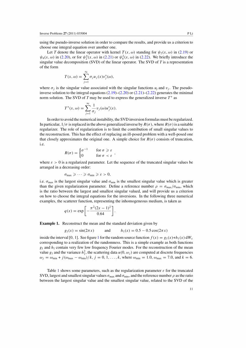
inside the interval [0, 1]. See figure 1 for the random source function f (x) = g1(x)+h1(x) dWx
corresponding to a realization of the randomness. This is a simple example as both functionsg1 and h1 contain very few low frequency Fourier modes. For the reconstruction of the meanvalue g1 and the variance h2
1, the scattering data u(0, ωj ) are computed at discrete frequenciesωj = ωmin + j (ωmax − ωmin)/k, j = 0, 1, . . . , k, where ωmin = 1.0, ωmax = 7.0, and k = 6.
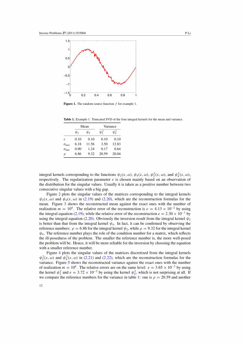
Table 1 shows some parameters, such as the regularization parameter ε for the truncatedSVD, largest and smallest singular values σmax and σmin, and the reference number ρ as the ratiobetween the largest singular value and the smallest singular value, related to the SVD of the
11
Inverse Problems 27 (2011) 035004 P Li
0 0.2 0.4 0.6 0.8 1−1.5
−1
−0.5
0
0.5
1
1.5
Figure 1. The random source function f for example 1.
Table 1. Example 1. Truncated SVD of the four integral kernels for the mean and variance.
Mean Variance
ψ2 ψ4 ψ22 ψ2
4
ε 0.10 0.10 0.10 0.10σmax 6.18 11.56 3.50 12.83σmin 0.90 1.24 0.17 0.64ρ 6.86 9.32 20.59 20.04
integral kernels corresponding to the functions ψ2(x, ω), ψ4(x, ω), ψ22 (x, ω), and ψ2
4 (x, ω),respectively. The regularization parameter ε is chosen mainly based on an observation ofthe distribution for the singular values. Usually it is taken as a positive number between twoconsecutive singular values with a big gap.
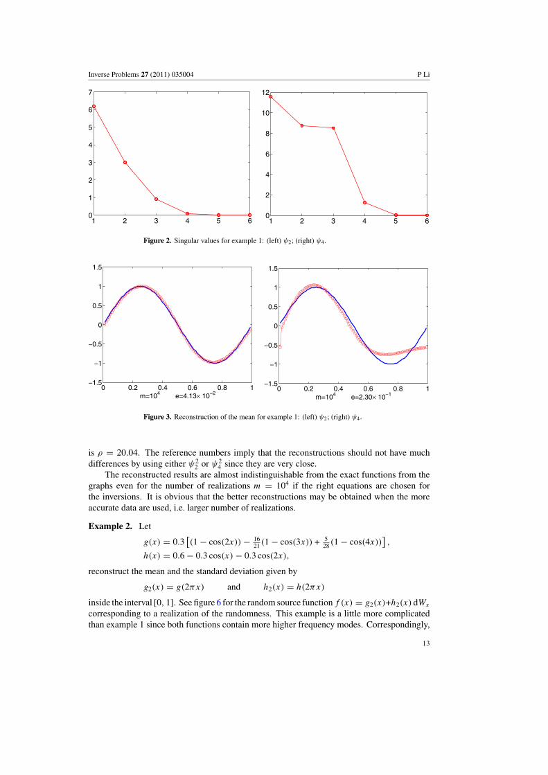
Figure 2 plots the singular values of the matrices corresponding to the integral kernelsψ2(x, ω) and ψ4(x, ω) in (2.19) and (2.20), which are the reconstruction formulas for themean. Figure 3 shows the reconstructed mean against the exact ones with the number ofrealization m = 104. The relative error of the reconstruction is e = 4.13 × 10⁻² by usingthe integral equation (2.19), while the relative error of the reconstruction e = 2.30 × 10⁻¹ byusing the integral equation (2.20). Obviously the inversion result from the integral kernel ψ2
is better than that from the integral kernel ψ4. In fact, it can be confirmed by observing thereference numbers: ρ = 6.86 for the integral kernel ψ2, while ρ = 9.32 for the integral kernelψ4. The reference number plays the role of the condition number for a matrix, which reflectsthe ill-posedness of the problem. The smaller the reference number is, the more well-posedthe problem will be. Hence, it will be more reliable for the inversion by choosing the equationwith a smaller reference number.
Figure 4 plots the singular values of the matrices discretized from the integral kernelsψ2
2 (x, ω) and ψ24 (x, ω) in (2.21) and (2.22), which are the reconstruction formulas for the
variance. Figure 5 shows the reconstructed variance against the exact ones with the numberof realization m = 104. The relative errors are on the same level: e = 3.65 × 10⁻² by usingthe kernel ψ2
2 and e = 3.72 × 10⁻² by using the kernel ψ24 , which is not surprising at all. If
we compare the reference numbers for the variance in table 1: one is ρ = 20.59 and another
12
Inverse Problems 27 (2011) 035004 P Li
1 2 3 4 5 60
1
2
3
4
5
6
7
1 2 3 4 5 60
2
4
6
8
10
12
Figure 2. Singular values for example 1: (left) ψ2; (right) ψ4.
0 0.2 0.4 0.6 0.8 1−1.5
−1
−0.5
0
0.5
1
1.5
m=104 e=4.13× 10⁻²⁰ 0.2 0.4 0.6 0.8 1
−1.5
−1
−0.5
0
0.5
1
1.5
m=104 e=2.30× 10⁻¹
Figure 3. Reconstruction of the mean for example 1: (left) ψ2; (right) ψ4.
is ρ = 20.04. The reference numbers imply that the reconstructions should not have muchdifferences by using either ψ2
2 or ψ24 since they are very close.
The reconstructed results are almost indistinguishable from the exact functions from thegraphs even for the number of realizations m = 104 if the right equations are chosen forthe inversions. It is obvious that the better reconstructions may be obtained when the moreaccurate data are used, i.e. larger number of realizations.
Example 2. Let
g(x) = 0.3[(1 − cos(2x)) − 16
21 (1 − cos(3x)) + 528 (1 − cos(4x))
],
h(x) = 0.6 − 0.3 cos(x) − 0.3 cos(2x),
reconstruct the mean and the standard deviation given by
g2(x) = g(2πx) and h2(x) = h(2πx)
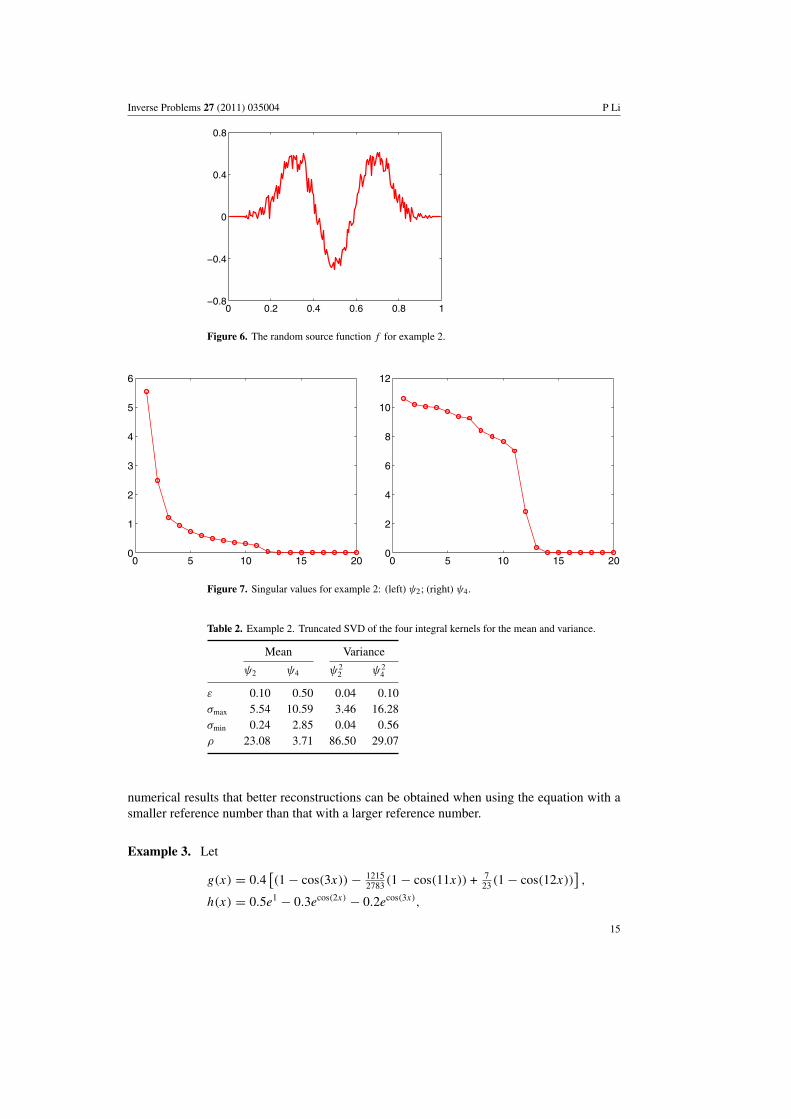
inside the interval [0, 1]. See figure 6 for the random source function f (x) = g2(x)+h2(x) dWx
corresponding to a realization of the randomness. This example is a little more complicatedthan example 1 since both functions contain more higher frequency modes. Correspondingly,
13

Inverse Problems 27 (2011) 035004 P Li
1 2 3 4 5 60
0.5
1
1.5
2
2.5
3
3.5
1 2 3 4 5 60
2
4
6
8
10
12
14
Figure 4. Singular values for example 1: (left) ψ22 ; (right) ψ2
4 .
0 0.2 0.4 0.6 0.8 1−0.4
0
0.4
0.8
1.2
m=104 e=3.65× 10⁻²⁰ 0.2 0.4 0.6 0.8 1
−0.4
0
0.4
0.8
1.2
m=104 e=3.72× 10⁻²
Figure 5. Reconstruction of the variance for example 1: (left) ψ22 ; (right) ψ2
4 .
the data at high frequencies should be computed to recover the mean g2 and the standarddeviation h2. For the reconstruction of the mean value g2, the scattering data u(0, ωj ) arecomputed at discrete frequencies ωj = ωmin + j (ωmax − ωmin)/k, j = 0, 1, . . . , k, whereωmin = 1.0, ωmax = 31.0, and k = 20; while the scattering data u(0, ωj ) are computed atfrequencies ωj = ωmin + j (ωmax − ωmin)/k, j = 1, 2, . . . , k, where ωmin = 1.0, ωmax = 11.0,and k = 10, for the reconstruction of the standard deviation h2.
Table 2 shows the regularization parameter, largest and smallest singular values,and the reference numbers for the truncated SVD of the kernels corresponding toψ2(x, ω), ψ4(x, ω), ψ2
2 (x, ω), and ψ24 (x, ω), respectively.
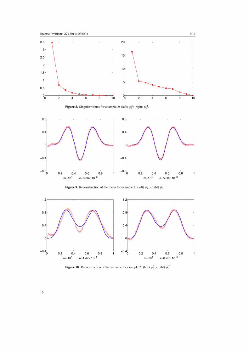
Figures 7 and 8 plot the singular values of the matrices corresponding to the integralkernels ψ2(x, ω) and ψ4(x, ω) in (2.19) and (2.20), and ψ2
2 (x, ω) and ψ24 (x, ω) in (2.21)
and (2.22), respectively. Figures 9 and 10 show the reconstructed mean and variance againstthe exact ones with the number of realization m = 104. The relative reconstruction errorsare e = 6.06 × 10⁻² (using ψ2 to reconstruct the mean) and e = 5.08 × 10⁻² (using ψ4
to reconstruct the mean), and e = 1.47 × 10⁻¹ (using ψ22 to reconstruct the variance) and
e = 6.78 × 10⁻² (using ψ24 to reconstruct the variance). Again, it is confirmed from the
14
Inverse Problems 27 (2011) 035004 P Li
0 0.2 0.4 0.6 0.8 1−0.8
−0.4
0
0.4
0.8
Figure 6. The random source function f for example 2.
0 5 10 15 200
1
2
3
4
5
6
0 5 10 15 200
2
4
6
8
10
12
Figure 7. Singular values for example 2: (left) ψ2; (right) ψ4.
Table 2. Example 2. Truncated SVD of the four integral kernels for the mean and variance.
Mean Variance
ψ2 ψ4 ψ22 ψ2
4
ε 0.10 0.50 0.04 0.10σmax 5.54 10.59 3.46 16.28σmin 0.24 2.85 0.04 0.56ρ 23.08 3.71 86.50 29.07
numerical results that better reconstructions can be obtained when using the equation with asmaller reference number than that with a larger reference number.
Example 3. Let
g(x) = 0.4[(1 − cos(3x)) − 1215
2783 (1 − cos(11x)) + 723 (1 − cos(12x))
],
h(x) = 0.5e1 − 0.3ecos(2x) − 0.2ecos(3x),
15
Inverse Problems 27 (2011) 035004 P Li
0 2 4 6 8 100
0.5
1
1.5
2
2.5
3
3.5
0 2 4 6 8 100
5
10
15
20
Figure 8. Singular values for example 2: (left) ψ22 ; (right) ψ2
4 .
0 0.2 0.4 0.6 0.8 1−0.8
−0.4
0
0.4
0.8
m=104 e=6.06× 10⁻²⁰ 0.2 0.4 0.6 0.8 1
−0.8
−0.4
0
0.4
0.8
m=104 e=5.08× 10⁻²
Figure 9. Reconstruction of the mean for example 2: (left) ψ2; (right) ψ4.
0 0.2 0.4 0.6 0.8 1−0.4
0
0.4
0.8
1.2
m=104 e=1.47× 10⁻¹⁰ 0.2 0.4 0.6 0.8 1
−0.4
0
0.4
0.8
1.2
m=104 e=6.78× 10⁻²
Figure 10. Reconstruction of the variance for example 2: (left) ψ22 ; (right) ψ2
4 .
16
Inverse Problems 27 (2011) 035004 P Li
0 0.2 0.4 0.6 0.8 1−0.8
−0.4
0
0.4
0.8
1.2
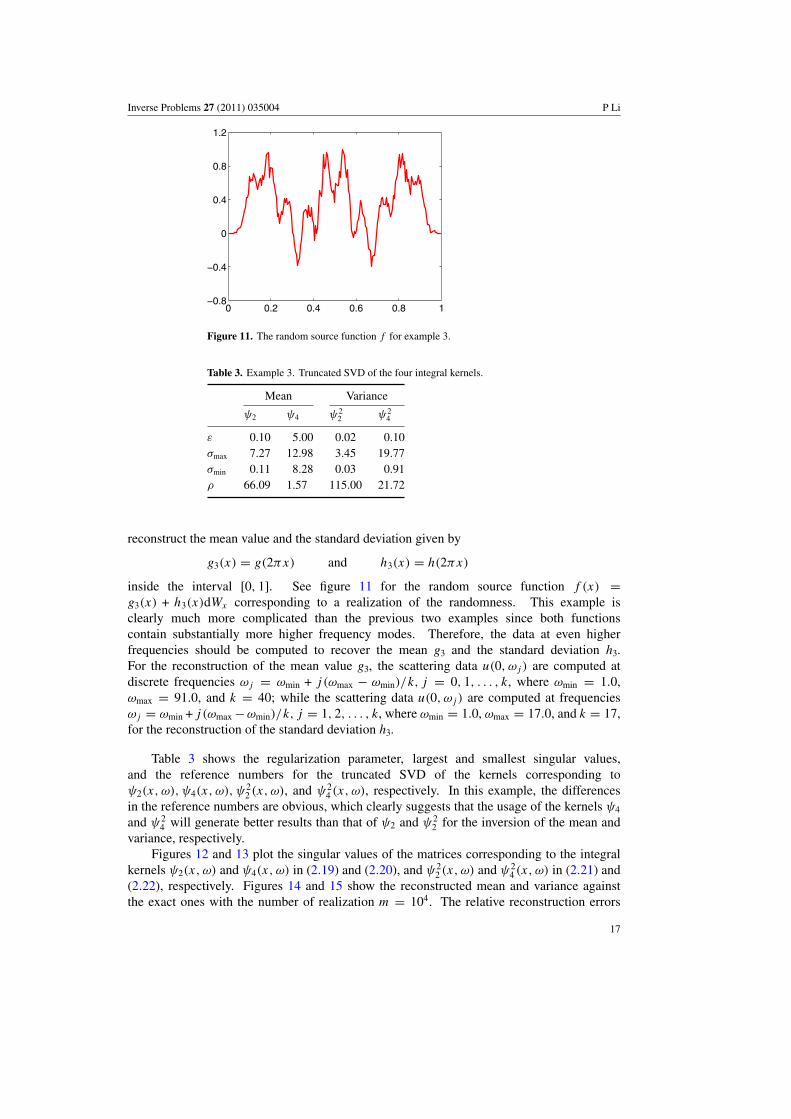
Figure 11. The random source function f for example 3.
Table 3. Example 3. Truncated SVD of the four integral kernels.
Mean Variance
ψ2 ψ4 ψ22 ψ2
4
ε 0.10 5.00 0.02 0.10σmax 7.27 12.98 3.45 19.77σmin 0.11 8.28 0.03 0.91ρ 66.09 1.57 115.00 21.72
reconstruct the mean value and the standard deviation given by
g3(x) = g(2πx) and h3(x) = h(2πx)
inside the interval [0, 1]. See figure 11 for the random source function f (x) =g3(x) + h3(x)dWx corresponding to a realization of the randomness. This example isclearly much more complicated than the previous two examples since both functionscontain substantially more higher frequency modes. Therefore, the data at even higherfrequencies should be computed to recover the mean g3 and the standard deviation h3.For the reconstruction of the mean value g3, the scattering data u(0, ωj ) are computed atdiscrete frequencies ωj = ωmin + j (ωmax − ωmin)/k, j = 0, 1, . . . , k, where ωmin = 1.0,ωmax = 91.0, and k = 40; while the scattering data u(0, ωj ) are computed at frequenciesωj = ωmin + j (ωmax −ωmin)/k, j = 1, 2, . . . , k, where ωmin = 1.0, ωmax = 17.0, and k = 17,for the reconstruction of the standard deviation h3.
Table 3 shows the regularization parameter, largest and smallest singular values,and the reference numbers for the truncated SVD of the kernels corresponding toψ2(x, ω), ψ4(x, ω), ψ2
2 (x, ω), and ψ24 (x, ω), respectively. In this example, the differences
in the reference numbers are obvious, which clearly suggests that the usage of the kernels ψ4
and ψ24 will generate better results than that of ψ2 and ψ2
2 for the inversion of the mean andvariance, respectively.
Figures 12 and 13 plot the singular values of the matrices corresponding to the integralkernels ψ2(x, ω) and ψ4(x, ω) in (2.19) and (2.20), and ψ2
2 (x, ω) and ψ24 (x, ω) in (2.21) and
(2.22), respectively. Figures 14 and 15 show the reconstructed mean and variance againstthe exact ones with the number of realization m = 104. The relative reconstruction errors
17

Inverse Problems 27 (2011) 035004 P Li
0 10 20 30 400
1
2
3
4
5
6
7
8
0 10 20 30 400
2
4
6
8
10
12
14
Figure 12. Singular values for example 3: (left) ψ2; (right) ψ4.
0 4 8 12 160
0.5
1
1.5
2
2.5
3
3.5
0 4 8 12 160
5
10
15
20
Figure 13. Singular values for example 3: (left) ψ22 ; (right) ψ2
4 .
0 0.2 0.4 0.6 0.8 1−0.8
−0.4
0
0.4
0.8
1.2
m=104 e=1.04× 10⁻¹⁰ 0.2 0.4 0.6 0.8 1
−0.8
−0.4
0
0.4
0.8
1.2
m=104 e=8.08× 10⁻²
Figure 14. Reconstruction of the mean for example 3: (left) ψ2; (right) ψ4.
are e = 1.01 × 10⁻¹ (using ψ2 to reconstruct the mean) and e = 8.08 × 10⁻² (using ψ4
to reconstruct the mean), and e = 1.07 × 10⁻¹ (using ψ22 to reconstruct the variance) and
e = 7.77 × 10⁻² (using ψ24 to reconstruct the variance). Once again, it is confirmed from the
18

Inverse Problems 27 (2011) 035004 P Li
0 0.2 0.4 0.6 0.8 1−0.4
0
0.4
0.8
1.2
1.6
m=104 e=1.07× 10⁻¹⁰ 0.2 0.4 0.6 0.8 1
−0.4
0
0.4
0.8
1.2
1.6
m=104 e=7.77× 10⁻²
Figure 15. Reconstruction of the variance for example 3: (left) ψ22 ; (right) ψ2
4 .
0 0.2 0.4 0.6 0.8 1−0.8
−0.4
0
0.4
0.8
1.2
m=105 e=2.79× 10⁻²⁰ 0.2 0.4 0.6 0.8 1
−0.4
0
0.4
0.8
1.2
1.6
m=105 e=3.62× 10⁻²
Figure 16. Reconstruction of the random source function for example 3 with the number ofrealization m = 105: (left) mean; (right) variance.
numerical results that better reconstructions can be obtained when using the equation with asmaller reference number than that with a larger reference number.
To show the effect of the number of the realization m on the reconstruction, figure 16shows the reconstructed mean (using ψ4) and variance (using ψ2
4 ) against the exact oneswith m = 105. The relative errors are e = 2.79 × 10⁻² for the mean (comparing the errore = 8.08 × 10⁻² when m = 104) and e = 3.62 × 10⁻² for the variance (comparing the errore = 7.77 × 10⁻² when m = 104). As expected, better results are obtained since a largernumber of realization intends to reduce the effect of data error.
Finally, to test the stability of the method, we reconstruct the mean and variance withnoisy data. Some relative random noise is added to the data, i.e. the scattering data take
u := (1 + δ rand)u.
Here, rand gives uniformly distributed random numbers in [−1, 1] and δ is a noise levelparameter. Figure 17 displays the reconstructed mean and variance with the scattering datacorresponding to the noisy level δ = 5% and the number of the realization m = 105. Itreconstructs the mean with a 8.81% relative error and the variance with a 5.86% relative error.
19

Inverse Problems 27 (2011) 035004 P Li
0 0.2 0.4 0.6 0.8 1−0.8
−0.4
0.5
0.4
0.8
1.2
m=105 e=8.81× 10⁻²⁰ 0.2 0.4 0.6 0.8 1
−0.4
0
0.4
0.8
1.2
1.6
m=105 e=5.86× 10⁻²
Figure 17. Reconstruction of the random source function for example 3 with noisy data: (left)mean; (right) variance.
An examination of the plot shows that the error of the reconstructions occurs largely aroundthe edges, while the middle parts of the functions are recovered more accurately.
In summary, the following observations can be made based on numerical experiments.When the functions contain few low Fourier modes or fast decaying Fourier coefficients,accurate and stable reconstructions can be obtained easily by using scattering data with lowfrequencies. To get better results, scattering data containing high frequencies should be used torecover the functions with high Fourier modes. Generally, the system with a smaller referencenumber will generate a better construction and a more reliable solution due to a relativelywell-posed nature of the problem.
4. Concluding remarks
We studied an inverse scattering problem for the stochastic Helmholtz equation with a randomsource function in a slab of the inhomogeneous medium. Both the direct and the inverseproblems were considered. The direct problem was equivalently formulated as a two-pointstochastic boundary value problem, and was shown having pathwise existence and uniquenessof a solution. Based on a constructed solution for the direct problem, the integral equationswere derived for the reconstruction formulas, which connect the mean value and varianceof the random source to those of the measured field. Numerical examples were presentedto demonstrate the validity and effectiveness of the proposed method. We are currentlyinvestigating the inverse random source scattering problem for the two- and three-dimensionalHelmholtz equation in homogeneous and inhomogeneous media and will report the progresselsewhere in the future.
Acknowledgments
The research was supported in part by NSF grants EAR-0724656, DMS-0914595, and DMS-1042958.
20
Inverse Problems 27 (2011) 035004 P Li
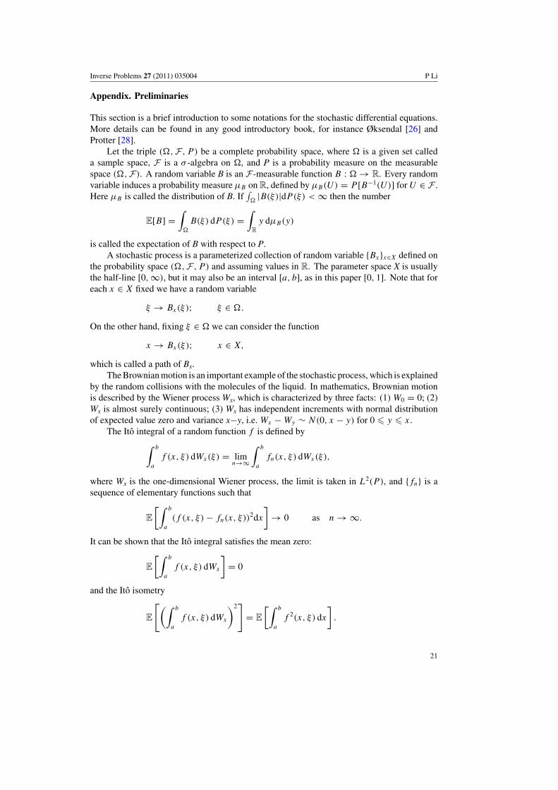
Appendix. Preliminaries
This section is a brief introduction to some notations for the stochastic differential equations.More details can be found in any good introductory book, for instance Øksendal [26] andProtter [28].
Let the triple ( ,F, P ) be a complete probability space, where is a given set calleda sample space, F is a σ -algebra on , and P is a probability measure on the measurablespace ( ,F). A random variable B is an F-measurable function B : → R. Every randomvariable induces a probability measure μB on R, defined by μB(U) = P [B−1(U)] for U ∈ F .Here μB is called the distribution of B. If
∫
|B(ξ)|dP(ξ) < ∞ then the number
E[B] =∫
B(ξ) dP(ξ) =∫
R
y dμB(y)
is called the expectation of B with respect to P.A stochastic process is a parameterized collection of random variable {Bx}x∈X defined on
the probability space ( ,F, P ) and assuming values in R. The parameter space X is usuallythe half-line [0,∞), but it may also be an interval [a, b], as in this paper [0, 1]. Note that foreach x ∈ X fixed we have a random variable
ξ → Bx(ξ); ξ ∈ .
On the other hand, fixing ξ ∈ we can consider the function
x → Bx(ξ); x ∈ X,
which is called a path of Bx.The Brownian motion is an important example of the stochastic process, which is explained
by the random collisions with the molecules of the liquid. In mathematics, Brownian motionis described by the Wiener process Wx, which is characterized by three facts: (1) W0 = 0; (2)Wx is almost surely continuous; (3) Wx has independent increments with normal distributionof expected value zero and variance x−y, i.e. Wx − Wy ∼ N(0, x − y) for 0 � y � x.
The Ito integral of a random function f is defined by∫ b
a
f (x, ξ) dWx(ξ) = limn→∞
∫ b
a
fn(x, ξ) dWx(ξ),
where Wx is the one-dimensional Wiener process, the limit is taken in L2(P ), and {fn} is asequence of elementary functions such that
E
[∫ b
a
(f (x, ξ) − fn(x, ξ))2dx
]→ 0 as n → ∞.
It can be shown that the Ito integral satisfies the mean zero:
E
[∫ b
a
f (x, ξ) dWx
]= 0
and the Ito isometry
E
[(∫ b
a
f (x, ξ) dWx
)2]
= E
[∫ b
a
f 2(x, ξ) dx
].
21
Inverse Problems 27 (2011) 035004 P Li
References
[1] Albanese R and Monk P 2006 The inverse source problem for Maxwell’s equations Inverse Problems 22 1023–35[2] Ammari H, Bao G and Fleming J 2002 An inverse source problem for Maxwell’s equations in
magnetoencephalography SIAM J. Appl. Math. 62 1369–82[3] Badieirostami M, Adibi A, Zhou H and Chow S 2007 Model for efficient simulation of spatially incoherent
light using the Wiener chaos expansion method Opt. Lett. 32 3188–90[4] Bal G and Ryzhik L 2003 Time reversal and refocusing in random media SIAM J. Appl. Math. 63 1475–98[5] Bao G, Chow S-N, Li P and Zhou H 2010 Numerical solution of an inverse medium scattering problem with a
stochastic source Inverse Problems 26 074014[6] Bao G, Chow S-N, Li P and Zhou H 2011 An inverse random source problem for the Helmholtz equation (in
preparation)[7] Bao G, Lin J and Triki F 2010 A multi-frequency inverse source problem J. Diff. Eqns. 249 3443–65[8] Bleistein N and Cohen J 1977 Nonuniqueness in the inverse source problem in acoustic and electromagnetics
J. Math. Phys. 18 194–201[9] Cao Y-Z, Zhang R and Zhang K 2007 Finite element and discontinuous Galerkin method for stochastic Helmholtz
equation in two- and three-dimensions J. Comput. Math. 26 702–15[10] Colton D and Kress R 1998 Inverse Acoustic and Electromagnetic Scattering Theory (Appl. Math. Sci. vol
93)2nd edn (Berlin: Springer)[11] Devaney A 1979 The inverse problem for random sources J. Math. Phys. 20 1687–91[12] Devaney A, Marengo E and Li M 2007 The inverse source problem in nonhomogeneous background media
SIAM J. Appl. Math. 67 1353–78[13] Devaney A and Sherman G 1982 Nonuniqueness in inverse source and scattering problems IEEE Trans. Antennas
Propag. 30 1034–7[14] Eller M and Valdivia N 2009 Acoustic source identification using multiple frequency information Inverse
Problems 25 115005[15] Fannjiang A C and Sølna K 2005 Superresolution and duality for time-reversal of waves in random media Phys.
Lett. A 352 22–9[16] Fouque J-P, Garnier J, Papanicolaou G C and Sølna K 2007 Wave Propagation and Time Reversal in Randomly
Layered Media (New York: Springer)[17] Hauer K-H, Kuhn L and Potthast R 2005 On uniqueness and non-uniqueness for current reconstruction from
magnetic fields Inverse Problems 21 955–67[18] Higham D 2001 An algorithmic introduction to numerical simulation of stochastic differential equations SIAM
Rev. 43 525–46[19] Ishimaru A 1978 Wave Propagation and Scattering in Random Media (New York: Academic)[20] Kaipio J and Somersalo E 2005 Statistical and Computational Inverse Problems (New York: Springer)[21] Kloeden P and Platen E 1992 Numerical Solution of Stochastic Differential Equations (New York: Springer)[22] Marengo E and Devaney A 1999 The inverse source problem of electromagnetics: linear inversion formulation
and minimum energy solution IEEE Trans. Antennas Propag. 47 410–2[23] Marengo E, Khodja M and Boucherif A 2008 Inverse source problem in nonhomogeneous background media:
II. Vector formulation and antenna substrate performance characterization SIAM J. Appl. Math. 69 81–110[24] Nualart D and Pardoux E 1991 Boundary value problems for stochastic differential equations Ann.
Probab. 19 1118–44[25] Ocone D and Pardoux E 1989 Linear stochastic differential equations with boundary conditions Probab. Theory
Relat. Fields 82 489–526[26] Øksendal B 2005 Stochastic Differential Equations: An Introduction with Applications 6th edn (Berlin:
Springer)[27] Papanicolaou G 1971 Wave propagation in a one-dimensional random medium SIAM J. Appl. Math. 21 13–8[28] Protter P 2005 Stochastic Integration and Differential Equations 2nd edn (Berlin: Springer)[29] Yuste R 2005 Fluorescence microscopy today Nat. Methods 2 902–4
22