Embed Size (px)
Citation preview
Bézier Curves and Surfaces (2)
Hongxin Zhang and Jieqing Feng
2006-12-07
State Key Lab of CAD&CGZhejiang University
12/07/2006 State Key Lab of CAD&CG 2
Contents
• Reparameterizing Bézier Curves• Bézier Control Polygons for a Cubic Curve• The Equations for a Bézier Curve of Arbitrary
Degree • Bézier Patches • Bézier Curves on Bézier Patches • Subdivision of Bézier Patches • A Matrix Representation of the Cubic Bézier Patch• Advanced Topics on Bézier Curves/Patches• Course Downloaded
12/07/2006 State Key Lab of CAD&CG 3
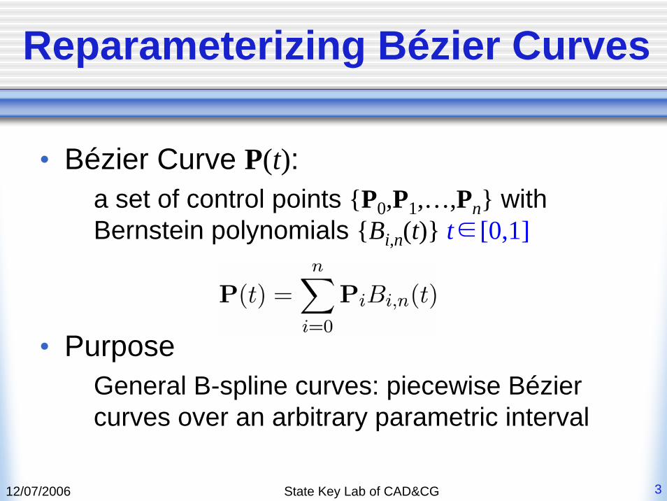
Reparameterizing Bézier Curves
• Bézier Curve P(t):a set of control points {P0,P1,…,Pn} with Bernstein polynomials {Bi,n(t)} t∈[0,1]
• PurposeGeneral B-spline curves: piecewise Bézier curves over an arbitrary parametric interval
12/07/2006 State Key Lab of CAD&CG 4
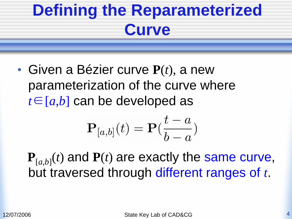
Defining the Reparameterized Curve
• Given a Bézier curve P(t), a new parameterization of the curve where t∈[a,b] can be developed as
P[a,b](t) and P(t) are exactly the same curve, but traversed through different ranges of t.
12/07/2006 State Key Lab of CAD&CG 5
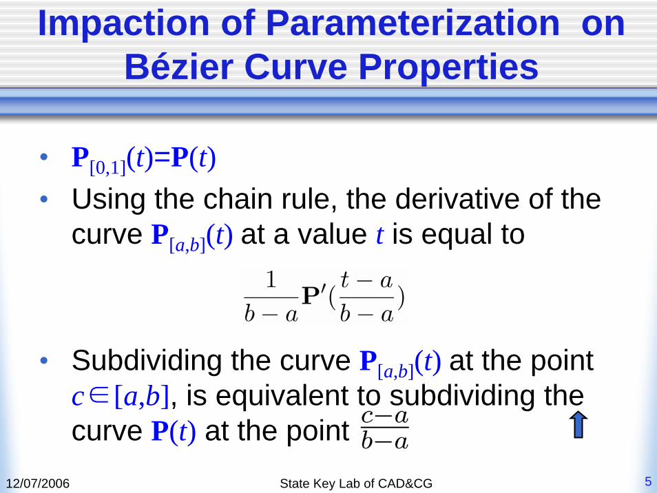
Impaction of Parameterization on Bézier Curve Properties
• P[0,1](t)=P(t)• Using the chain rule, the derivative of the
curve P[a,b](t) at a value t is equal to
• Subdividing the curve P[a,b](t) at the point c∈[a,b], is equivalent to subdividing the curve P(t) at the point
12/07/2006 State Key Lab of CAD&CG 6
Bézier Control Polygons for a Cubic Curve
• A Matrix Equation for a Cubic Curve• Reparameterization using the Matrix Form• A Specific Example• An Expanded Example
12/07/2006 State Key Lab of CAD&CG 7
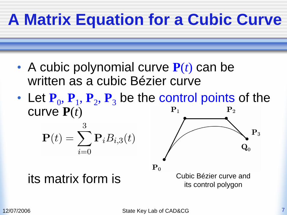
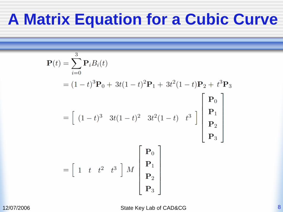
A Matrix Equation for a Cubic Curve
• A cubic polynomial curve P(t) can be written as a cubic Bézier curve
• Let P0, P1, P2, P3 be the control points of the curve P(t)
its matrix form is Cubic Bézier curve and its control polygon
12/07/2006 State Key Lab of CAD&CG 8
A Matrix Equation for a Cubic Curve
12/07/2006 State Key Lab of CAD&CG 9
A Matrix Equation for a Cubic Curve
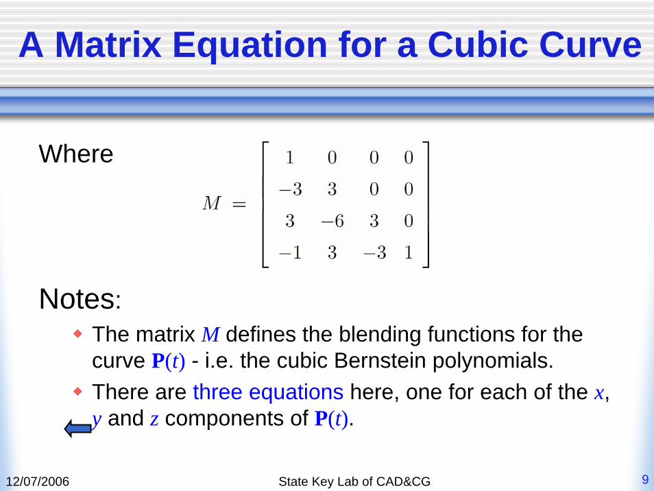
Where
Notes:The matrix M defines the blending functions for the curve P(t) - i.e. the cubic Bernstein polynomials. There are three equations here, one for each of the x, y and z components of P(t).
12/07/2006 State Key Lab of CAD&CG 10
Reparameterization using the Matrix Form
• Let P0, P1, P2, P3 be the control points of the curve P(t)
In general, the used parametric interval is [0,1]P0=P(0), P1=P(1)
• Given an interval [a,b], there exists a unique control polygon {Q0, Q1, Q2, Q3 }defining a Bézier curve Q(t), such that Q(0)=Q0=P(a) and Q(1)=Q1=P(b)
12/07/2006 State Key Lab of CAD&CG 11
Reparameterization using the Matrix Form
• Purpose: finding the Bézier polygon for the portion of the curve P(t) where t∈[a,b]
• Solution: by reparameterization and by manipulating the matrix representationabove
12/07/2006 State Key Lab of CAD&CG 12
Reparameterization using the Matrix Form
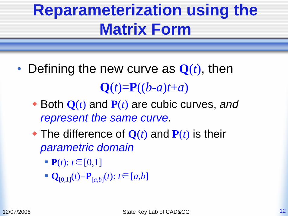
• Defining the new curve as Q(t), thenQ(t)=P((b-a)t+a)
Both Q(t) and P(t) are cubic curves, and represent the same curve.The difference of Q(t) and P(t) is their parametric domain
P(t): t∈[0,1]Q[0,1](t)=P[a,b](t): t∈[a,b]
12/07/2006 State Key Lab of CAD&CG 13
Reparameterization using the Matrix Form
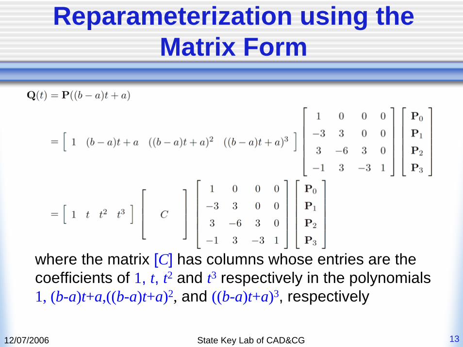
where the matrix [C] has columns whose entries are the coefficients of 1, t, t2 and t3 respectively in the polynomials 1, (b-a)t+a,((b-a)t+a)2, and ((b-a)t+a)3, respectively
12/07/2006 State Key Lab of CAD&CG 14
Reparameterization using the Matrix Form
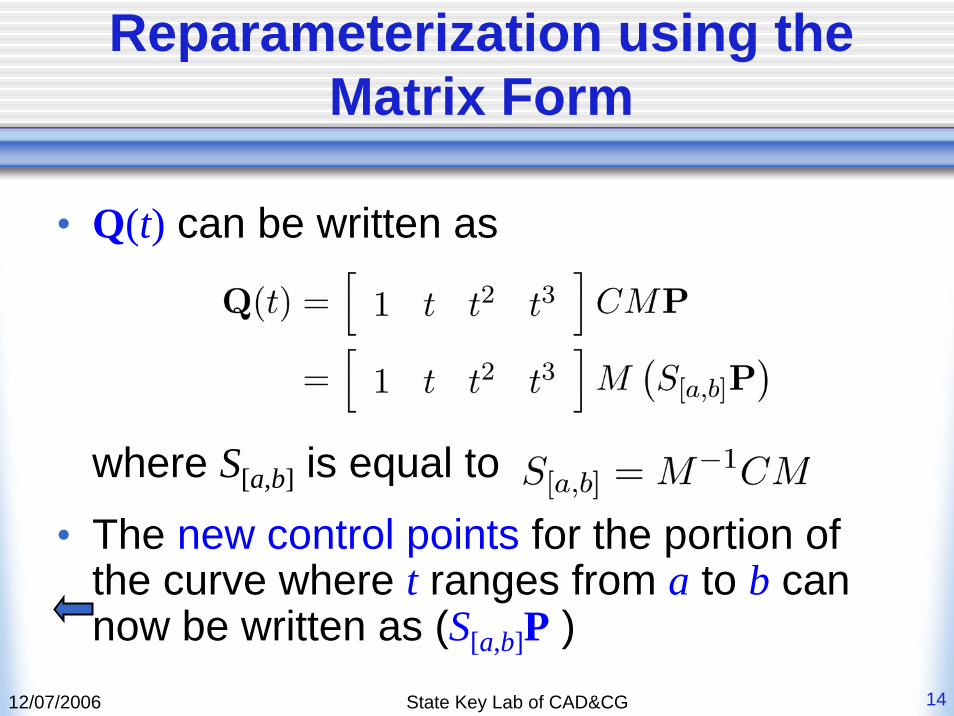
• Q(t) can be written as
where S[a,b] is equal to
• The new control points for the portion of the curve where t ranges from a to b can now be written as (S[a,b]P )
12/07/2006 State Key Lab of CAD&CG 15
A Specific Example
• P(t): parameter ranges from 1 to 2It is natural extension of P(t) from [0,1] to [1,2]It is useful to learn how to piece together two Bézier curves: The general B-spline curves are piecewise Bézier curves which are smoothly joined.

12/07/2006 State Key Lab of CAD&CG 16
Matrix Representation of P(t) on [1,2]
12/07/2006 State Key Lab of CAD&CG 17
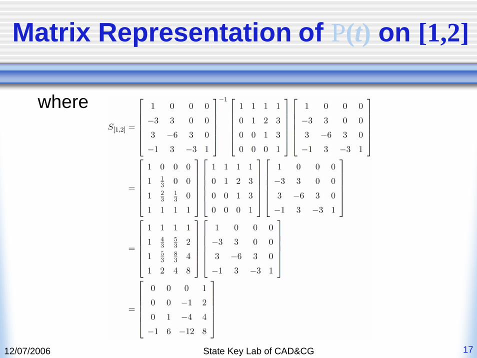
Matrix Representation of P(t) on [1,2]
where
12/07/2006 State Key Lab of CAD&CG 18
Matrix Representation of P(t) on [1,2]
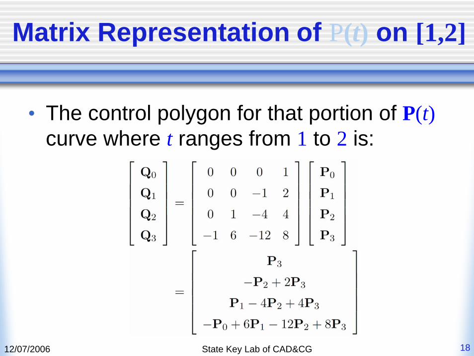
• The control polygon for that portion of P(t)curve where t ranges from 1 to 2 is:
12/07/2006 State Key Lab of CAD&CG 19
Geometric Interpretation of the New Control Points {Q0, Q1, Q2, Q3 }
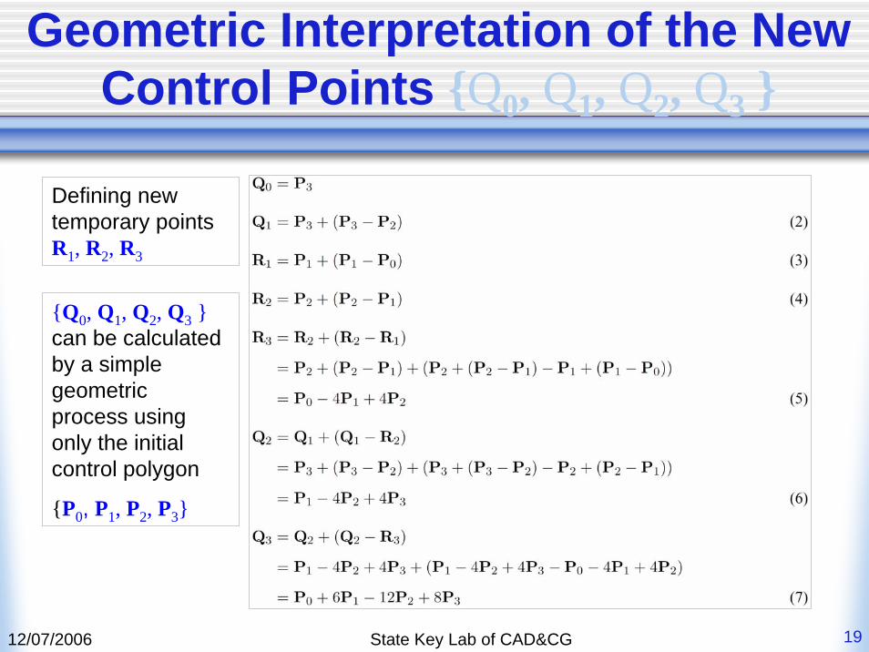
Defining new temporary points R1, R2, R3
{Q0, Q1, Q2, Q3 }can be calculated by a simple geometric process using only the initial control polygon
{P0, P1, P2, P3}
12/07/2006 State Key Lab of CAD&CG 20
Geometric Interpretation of the Q0 (1)
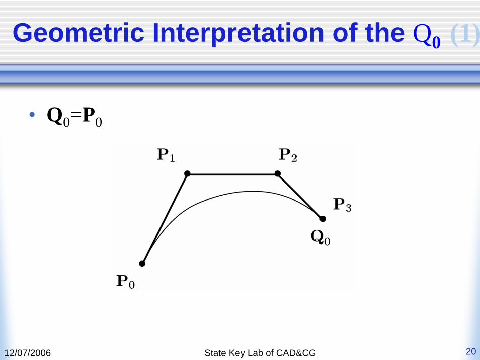
• Q0=P0
12/07/2006 State Key Lab of CAD&CG 21
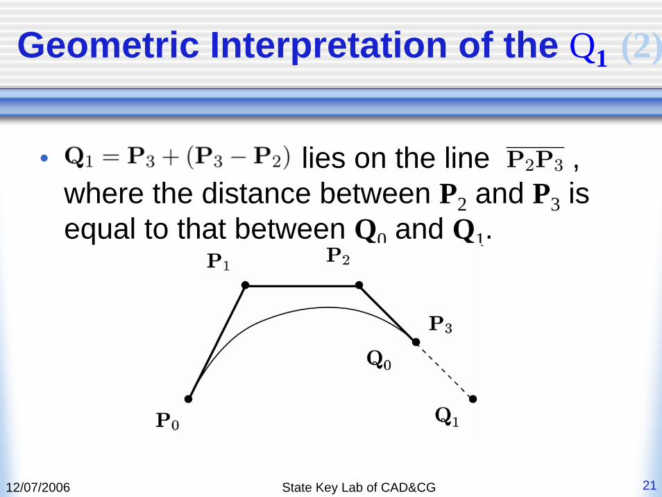
Geometric Interpretation of the Q1 (2)
• lies on the line , where the distance between P2 and P3 is equal to that between Q0 and Q1.
12/07/2006 State Key Lab of CAD&CG 22
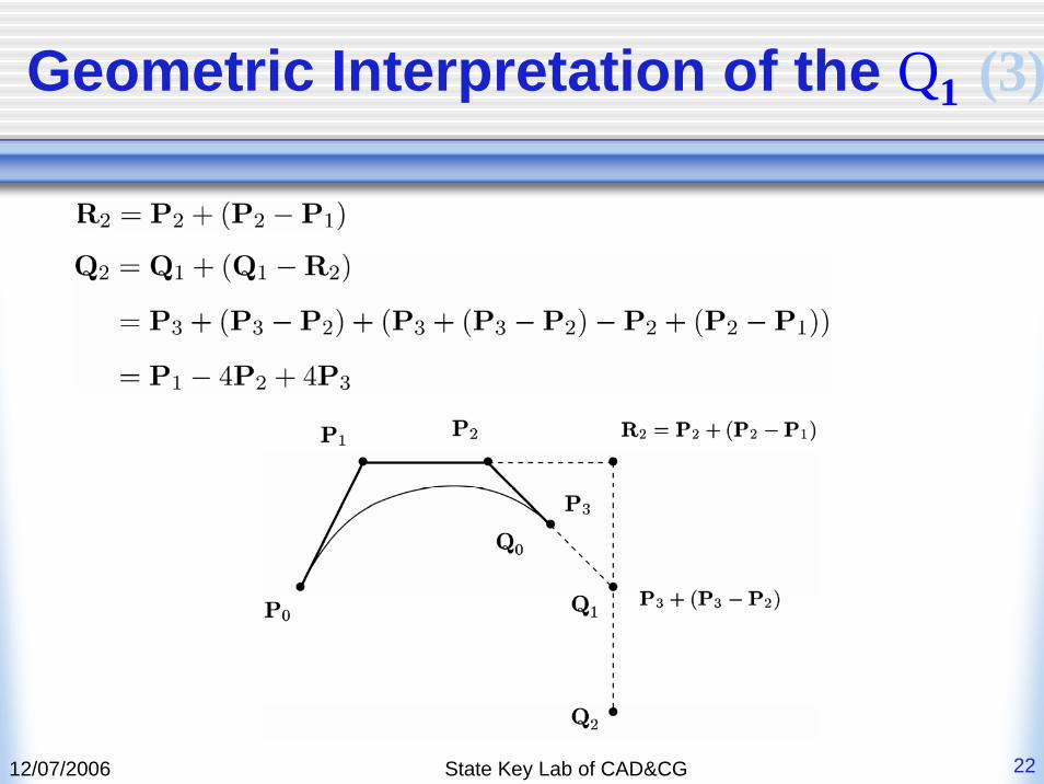
Geometric Interpretation of the Q1 (3)
12/07/2006 State Key Lab of CAD&CG 23
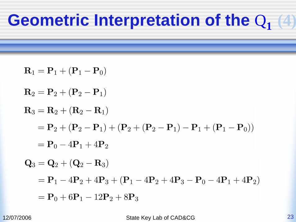
Geometric Interpretation of the Q1 (4)
12/07/2006 State Key Lab of CAD&CG 24
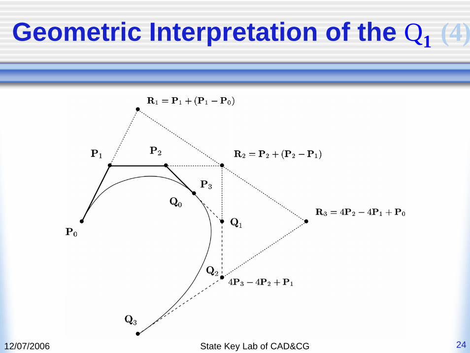
Geometric Interpretation of the Q1 (4)
12/07/2006 State Key Lab of CAD&CG 25
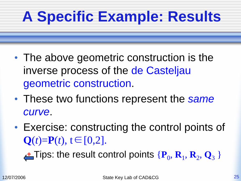
A Specific Example: Results
• The above geometric construction is the inverse process of the de Casteljau geometric construction.
• These two functions represent the same curve.
• Exercise: constructing the control points of Q(t)=P(t), t∈[0,2].
Tips: the result control points {P0, R1, R2, Q3 }
12/07/2006 State Key Lab of CAD&CG 26
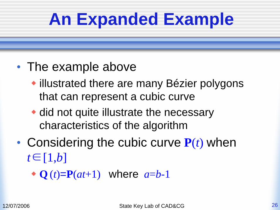
An Expanded Example
• The example above illustrated there are many Bézier polygons that can represent a cubic curvedid not quite illustrate the necessary characteristics of the algorithm
• Considering the cubic curve P(t) whent∈[1,b]
Q (t)=P(at+1) where a=b-1
12/07/2006 State Key Lab of CAD&CG 27
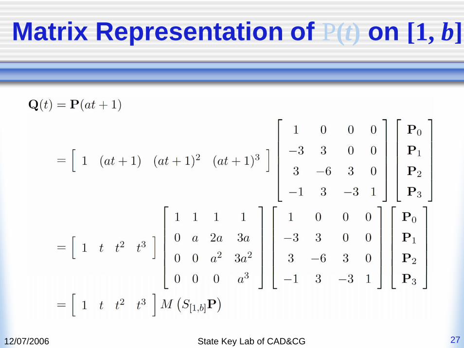
Matrix Representation of P(t) on [1, b]
12/07/2006 State Key Lab of CAD&CG 28
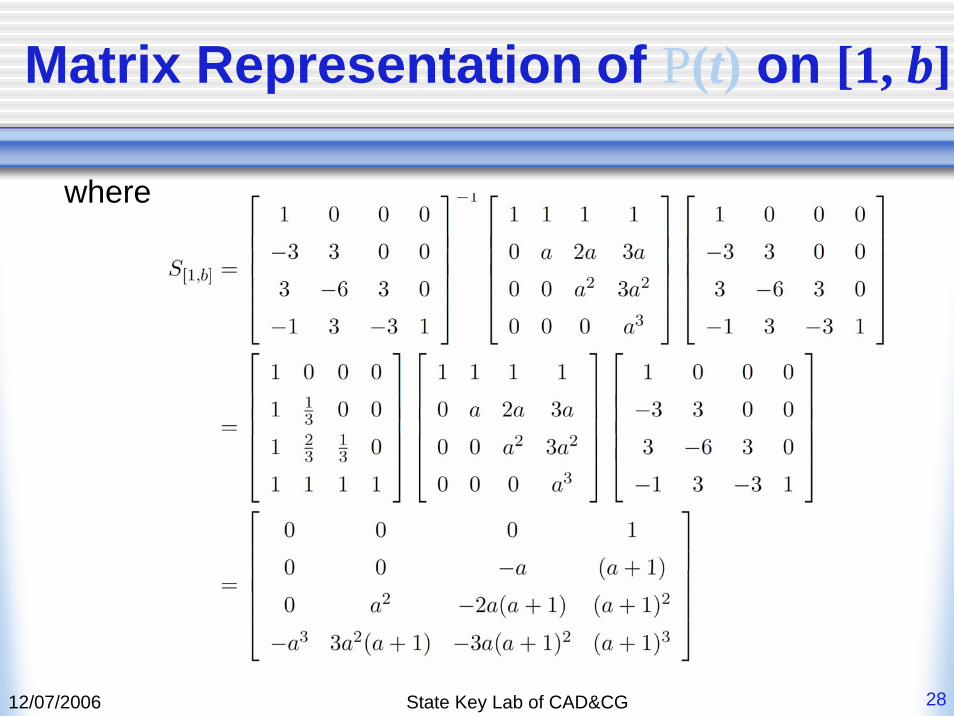
Matrix Representation of P(t) on [1, b]
where
12/07/2006 State Key Lab of CAD&CG 29
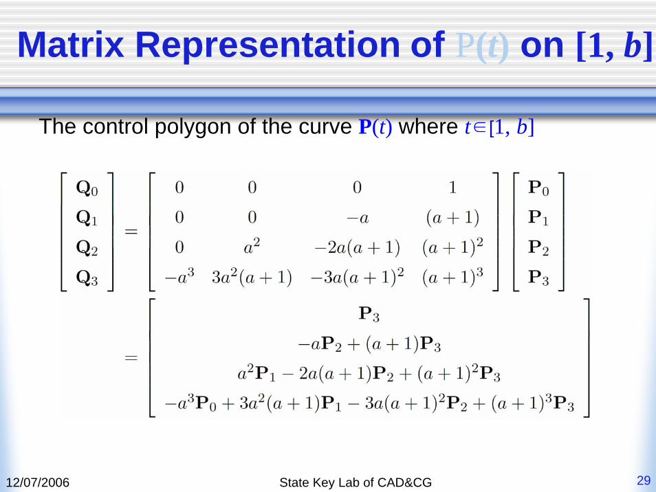
Matrix Representation of P(t) on [1, b]
The control polygon of the curve P(t) where t∈[1, b]
12/07/2006 State Key Lab of CAD&CG 30
Geometric Interpretation of the New Control Points {Q0, Q1, Q2, Q3 }
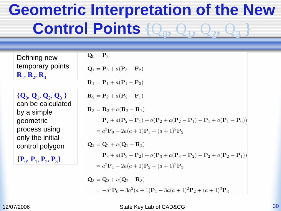
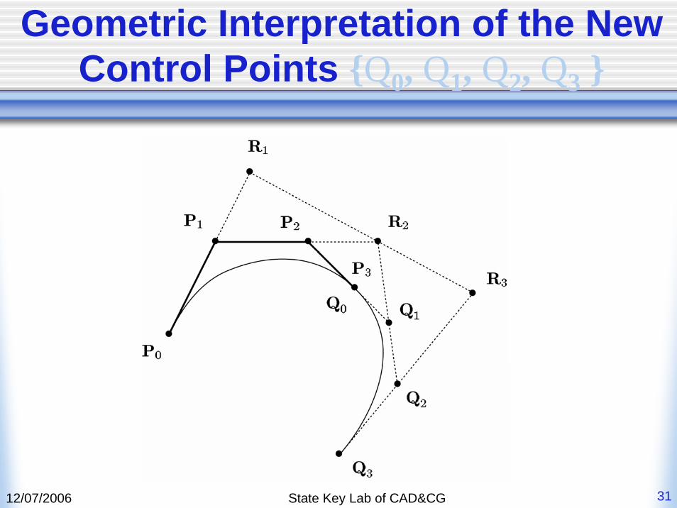
Defining new temporary points R1, R2, R3
{Q0, Q1, Q2, Q3 }can be calculated by a simple geometric process using only the initial control polygon
{P0, P1, P2, P3}
12/07/2006 State Key Lab of CAD&CG 31
Geometric Interpretation of the New Control Points {Q0, Q1, Q2, Q3 }
12/07/2006 State Key Lab of CAD&CG 32
Geometric Interpretation of the New Control Points {Q0, Q1, Q2, Q3 }
• ResultsThe important factor here is the a termEach of these points is on an extension of a line of the original control polygon, or the extension of a constructed lineThe factor a determines how much to extend.
12/07/2006 State Key Lab of CAD&CG 33
The Equations for a Bézier Curve of Arbitrary Degree
• OverviewThe Bézier curve representation is one that is utilized most frequently in computer graphics and geometric modeling. The curve is defined geometrically, which means that the parameters have geometric meaning - they are just points in three-dimensional space.It was developed by two competing European engineers in the late 1960s to attempt to draw automotive components.
12/07/2006 State Key Lab of CAD&CG 34
The Equations for a Bézier Curve of Arbitrary Degree
• Specification of the Bézier Curve of Arbitrary Degree
Generalizing the development for the quadratic and cubic Bézier curves Given the set of control points, {P0,P1,…,Pn }, defining a Bézier curve of degree n by either Analytic Definition or Geometric Construction.
12/07/2006 State Key Lab of CAD&CG 35
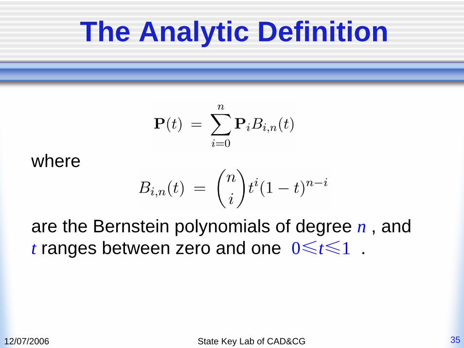
The Analytic Definition
where
are the Bernstein polynomials of degree n , and t ranges between zero and one 0≤t≤1 .
12/07/2006 State Key Lab of CAD&CG 36
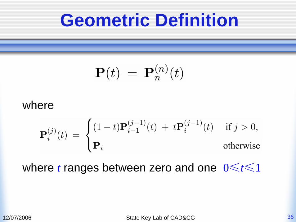
Geometric Definition
where
where t ranges between zero and one 0≤t≤1
12/07/2006 State Key Lab of CAD&CG 37
Properties of the Bézier Curve
• P0 and Pn are on the curve. • The curve is continuous and has continuous
derivatives of all orders. • The tangent line to the curve at the point P0 is the line
P0 P1. The tangent to the curve at the point Pn is the line Pn-1Pn .
• The curve lies within the convex hull of its control points. This is because each successive is a convex combination of the points and .
• P0,P1,…,Pn are all on the curve only if the curve is linear.
12/07/2006 State Key Lab of CAD&CG 38
Summary of the Bézier Curve
• Given a sequence of n+1 control points, one can specify a Bézier curve of degree n defined by these points.
• Two definitions of the curve can be given: An analytic definition specifying the blending of the control points with Bernstein polynomialsA geometric definition specifying a recursive generation procedure that calculates successive points on line segments developed from the control point sequence.
12/07/2006 State Key Lab of CAD&CG 39
Bézier Patches
• OverviewPierre Bézier in Renault and Paul de Casteljau in Citroën, initially developed a Bézier curve representation and extended it to a surface patch methodology
The extension of Bézier curves to surfaces is called the Bézier patch
The Bézier patch is the most commonly used surface representation in computer graphics
12/07/2006 State Key Lab of CAD&CG 40
Bézier Patches
• Bézier curve and patchThe Bézier curve is a function of one variableand takes a sequence of control points. The Bézier patch is a function of two variableswith an array of control points. Most of the methods for the patch are direct extensions of those for the curves.
12/07/2006 State Key Lab of CAD&CG 41
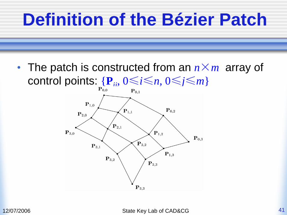
Definition of the Bézier Patch
• The patch is constructed from an n×m array of control points: {Pij, 0≤i≤n, 0≤j≤m}
12/07/2006 State Key Lab of CAD&CG 42
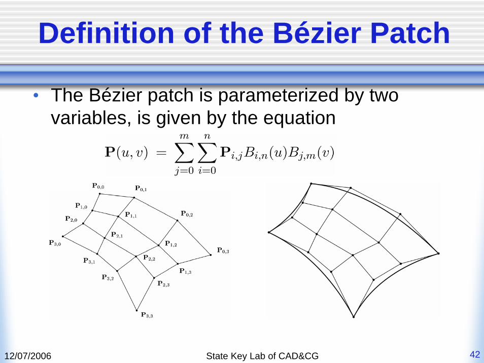
Definition of the Bézier Patch
• The Bézier patch is parameterized by two variables, is given by the equation
12/07/2006 State Key Lab of CAD&CG 43
Definition of the Bézier Patch
• It is summations running over all the control points
• The bi-variate Bernstein Polynomials serving as the functions that blend the control points together
Bi,n(u)Bj,m(v)
12/07/2006 State Key Lab of CAD&CG 44
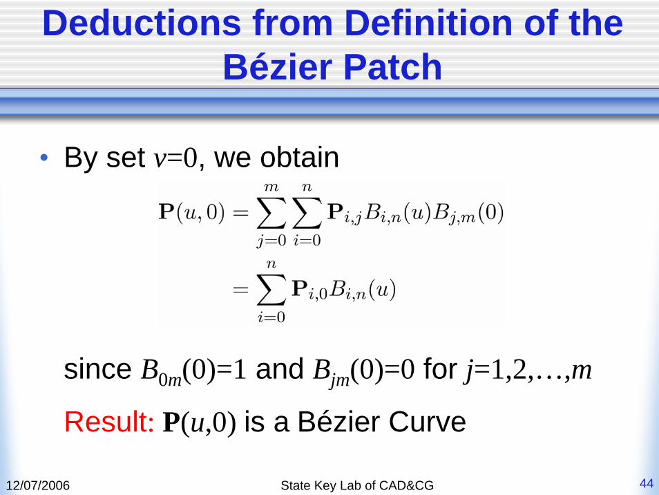
Deductions from Definition of the Bézier Patch
• By set v=0, we obtain
since B0m(0)=1 and Bjm(0)=0 for j=1,2,…,m
Result: P(u,0) is a Bézier Curve
12/07/2006 State Key Lab of CAD&CG 45
Deductions from Definition of the Bézier Patch
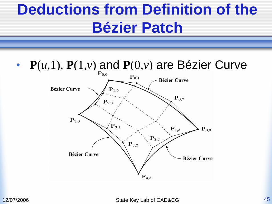
• P(u,1), P(1,v) and P(0,v) are Bézier Curve
12/07/2006 State Key Lab of CAD&CG 46
Relations between the Bézier Curve and Patch
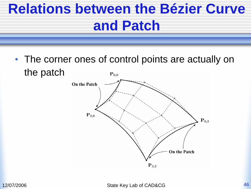
• The corner ones of control points are actually on the patch
12/07/2006 State Key Lab of CAD&CG 47
Properties of the Bézier Patch
• The four points P0,0, P0,m, Pn,0 and Pn,m are on the patch. The other control points are all on the patch only if the patch is planar.
• The patch is continuous and partial derivatives of all orders exist and are continuous.
• The patch lies within the convex hull of its control points.
12/07/2006 State Key Lab of CAD&CG 48
Bézier Curves on Bézier Patches
• OverviewP(0,v) and P(1,v) are Bézier curves lying on the boundary of the Bézier patch. A Bézier patch can be treated as a continuous set of Bézier curves. That is, for any fixed parameter u0 or v0 we can define a Bézier curve that lies directly on the surface of the patch. It is a very valuable tool for calculations on the patch
12/07/2006 State Key Lab of CAD&CG 49
Bézier Curves on Bézier Patches
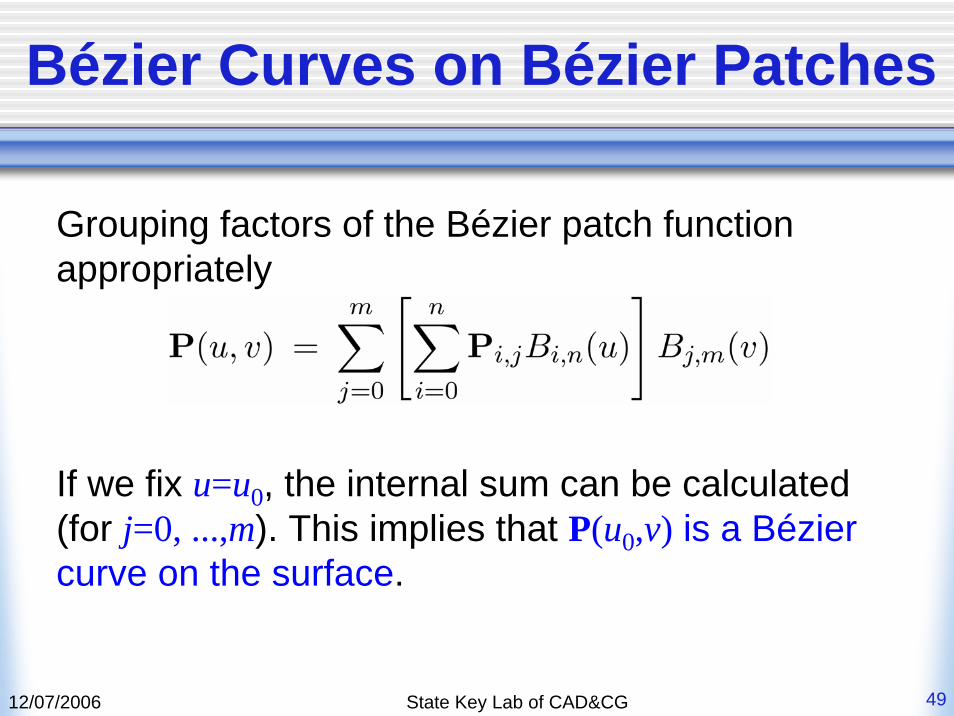
Grouping factors of the Bézier patch function appropriately
If we fix u=u0, the internal sum can be calculated (for j=0, ...,m). This implies that P(u0,v) is a Bézier curve on the surface.
12/07/2006 State Key Lab of CAD&CG 50
Bézier Curves on Bézier Patches
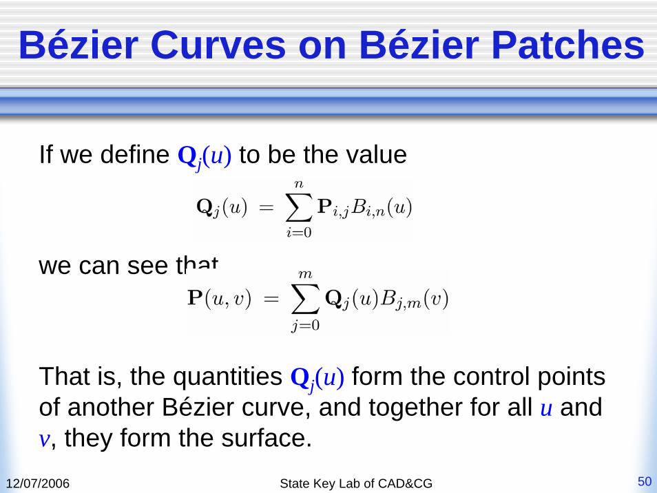
If we define Qj(u) to be the value
we can see that
That is, the quantities Qj(u) form the control points of another Bézier curve, and together for all u and v, they form the surface.
12/07/2006 State Key Lab of CAD&CG 51
Bézier Curves on Bézier Patches
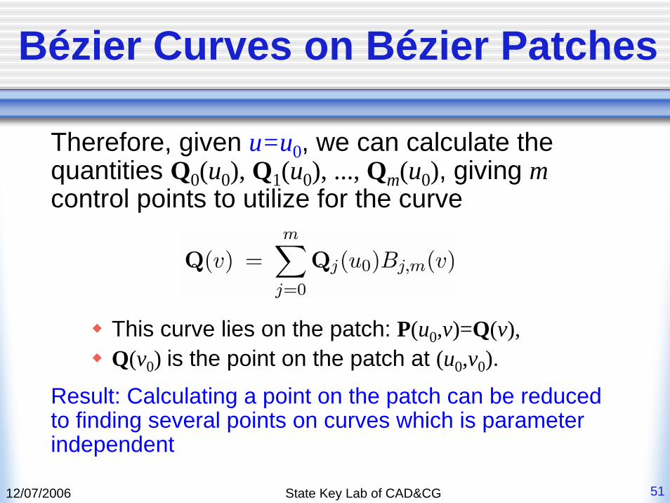
Therefore, given u=u0, we can calculate the quantities Q0(u0), Q1(u0), ..., Qm(u0), giving mcontrol points to utilize for the curve
This curve lies on the patch: P(u0,v)=Q(v),Q(v0) is the point on the patch at (u0,v0).
Result: Calculating a point on the patch can be reduced to finding several points on curves which is parameter independent

12/07/2006 State Key Lab of CAD&CG 52
Calculating a Point on a Bi-Cubic Surface: STEP 1
The point Q0(u0), is calculated as a point on the Béziercurve defined by the control points P0,0, P0,1, P0,2 and P0,3.
12/07/2006 State Key Lab of CAD&CG 53
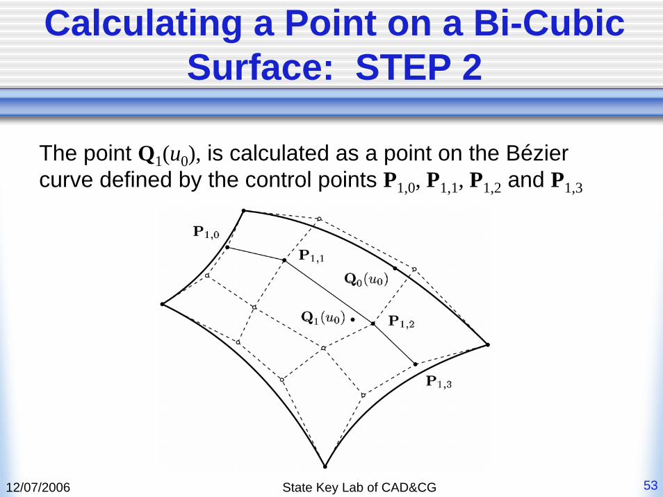
Calculating a Point on a Bi-Cubic Surface: STEP 2
The point Q1(u0), is calculated as a point on the Béziercurve defined by the control points P1,0, P1,1, P1,2 and P1,3
12/07/2006 State Key Lab of CAD&CG 54
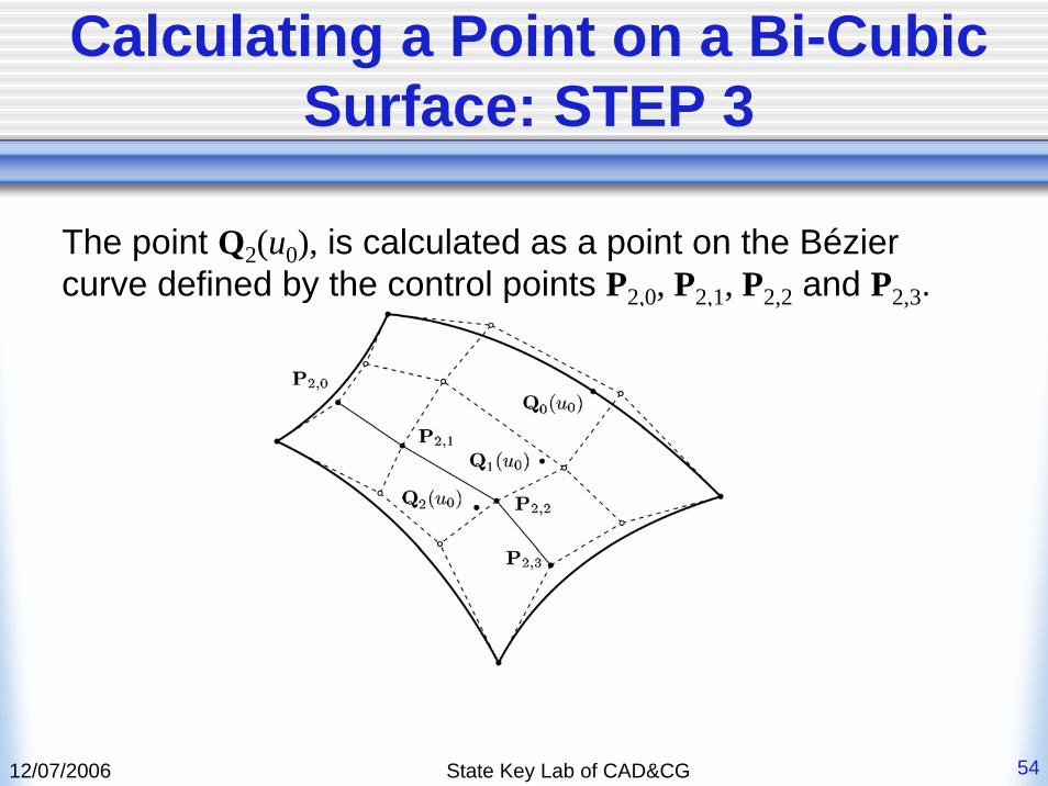
Calculating a Point on a Bi-Cubic Surface: STEP 3
The point Q2(u0), is calculated as a point on the Béziercurve defined by the control points P2,0, P2,1, P2,2 and P2,3.
12/07/2006 State Key Lab of CAD&CG 55
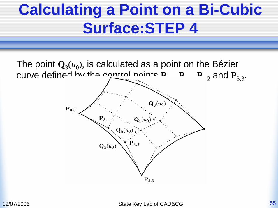
Calculating a Point on a Bi-Cubic Surface:STEP 4
The point Q3(u0), is calculated as a point on the Béziercurve defined by the control points P3,0, P3,1, P3,2 and P3,3.
12/07/2006 State Key Lab of CAD&CG 56
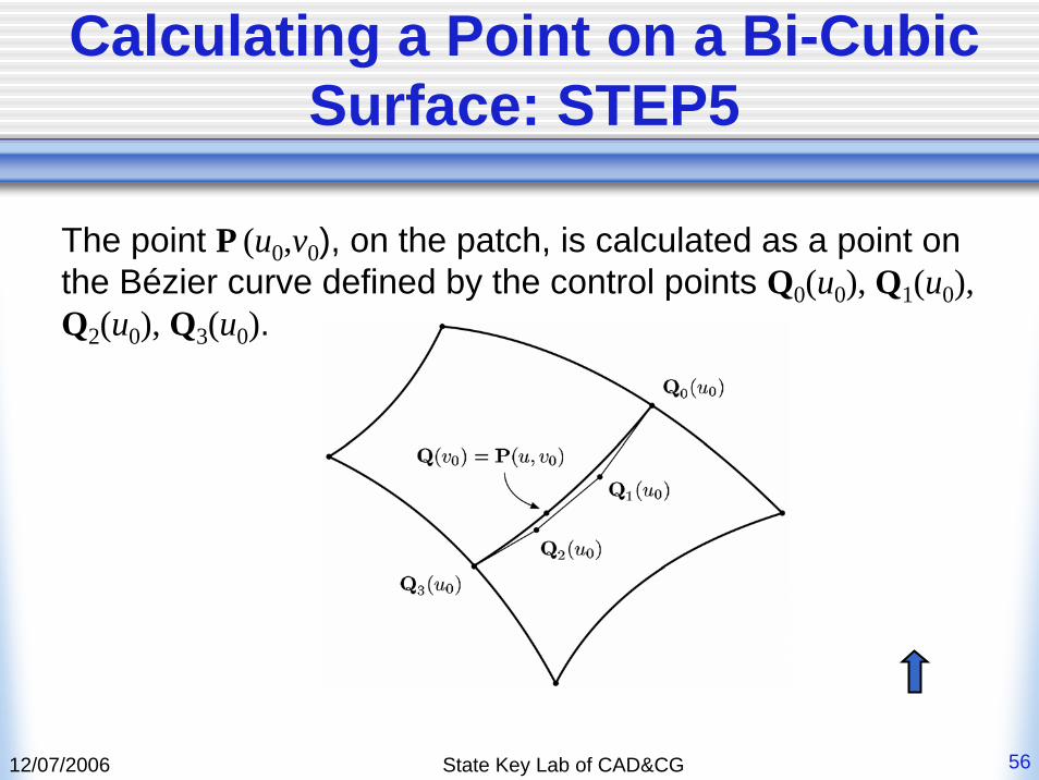
Calculating a Point on a Bi-Cubic Surface: STEP5
The point P (u0,v0), on the patch, is calculated as a point on the Bézier curve defined by the control points Q0(u0), Q1(u0), Q2(u0), Q3(u0).
12/07/2006 State Key Lab of CAD&CG 57
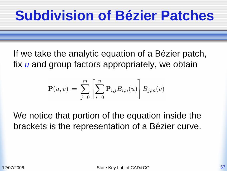
Subdivision of Bézier Patches
If we take the analytic equation of a Bézier patch, fix u and group factors appropriately, we obtain
We notice that portion of the equation inside the brackets is the representation of a Bézier curve.
12/07/2006 State Key Lab of CAD&CG 58
Subdivision of Bézier Patches
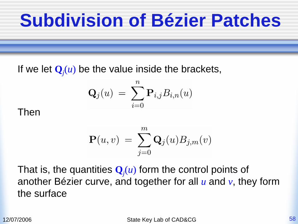
If we let Qj(u) be the value inside the brackets,
Then
That is, the quantities Qj(u) form the control points of another Bézier curve, and together for all u and v, they form the surface
12/07/2006 State Key Lab of CAD&CG 59
Subdivision of Bézier Patches
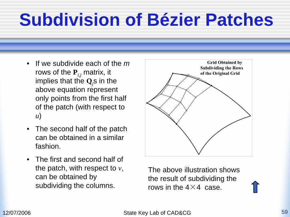
• If we subdivide each of the mrows of the Pi,j matrix, it implies that the Qjs in the above equation represent only points from the first half of the patch (with respect to u)
• The second half of the patch can be obtained in a similar fashion.
• The first and second half of the patch, with respect to v, can be obtained by subdividing the columns.
The above illustration shows the result of subdividing the rows in the 4×4 case.
12/07/2006 State Key Lab of CAD&CG 60
A Matrix Representation of the Cubic Bézier Patch
• Overview• Developing the Matrix Formulation • Patch Subdivision Using the Matrix Form • Calculation of the Second Half of the
Patch • General Subdivision with either Parameter
12/07/2006 State Key Lab of CAD&CG 61
Overview
• The matrix representation of the cubic Bézier patch allows us to specify many operations with Bézier patches
• The matrix operations can be performed quickly on computer systems optimized for geometry operations with matrices
12/07/2006 State Key Lab of CAD&CG 62
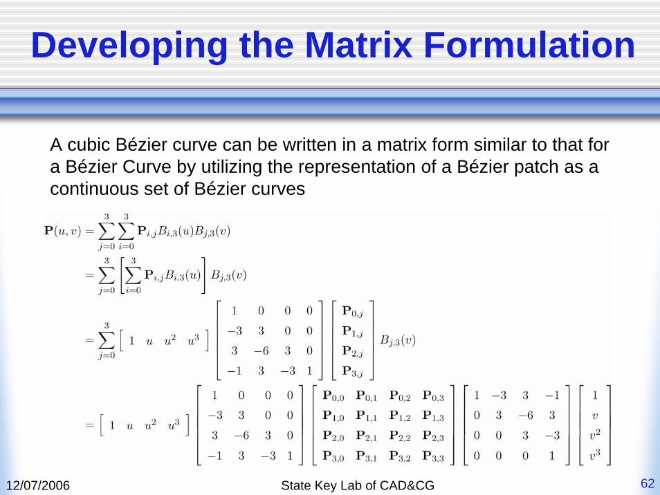
Developing the Matrix Formulation
A cubic Bézier curve can be written in a matrix form similar to that for a Bézier Curve by utilizing the representation of a Bézier patch as a continuous set of Bézier curves
12/07/2006 State Key Lab of CAD&CG 63
Developing the Matrix Formulation
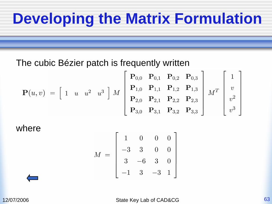
The cubic Bézier patch is frequently written
where
12/07/2006 State Key Lab of CAD&CG 64
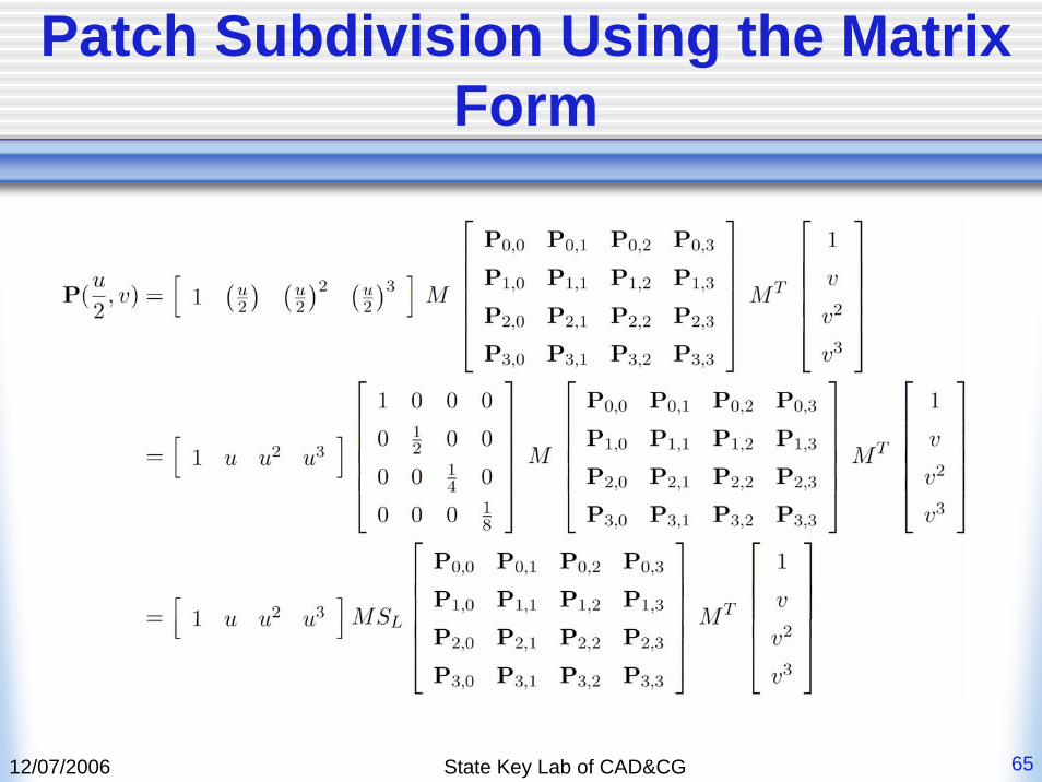
Patch Subdivision Using the Matrix Form
• Purpose: subdividing the patch at the point u=1/2
• Method: reparameterizing the matrix equation above (by substituting u/2 for u) to cover only the first half of the patch, and simplify to obtain.
12/07/2006 State Key Lab of CAD&CG 65
Patch Subdivision Using the Matrix Form
12/07/2006 State Key Lab of CAD&CG 66
Patch Subdivision Using the Matrix Form
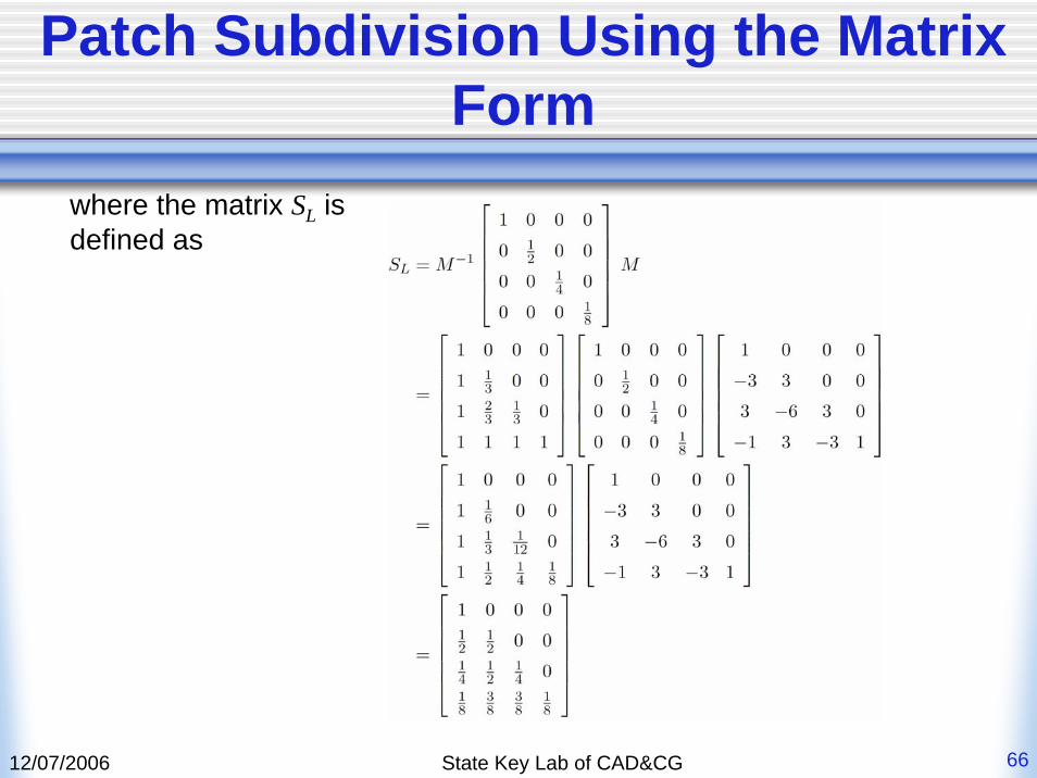
where the matrix SL is defined as
12/07/2006 State Key Lab of CAD&CG 67
Patch Subdivision Using the Matrix Form
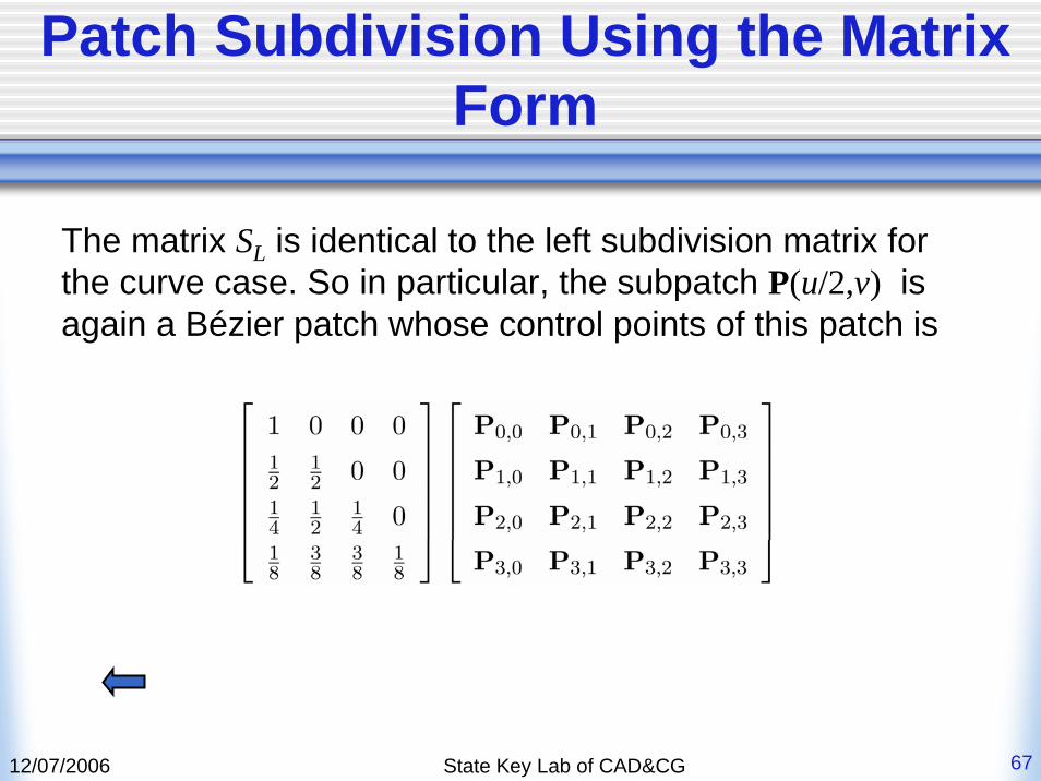
The matrix SL is identical to the left subdivision matrix for the curve case. So in particular, the subpatch P(u/2,v) is again a Bézier patch whose control points of this patch is
12/07/2006 State Key Lab of CAD&CG 68
Calculation of the Second Half of the Patch
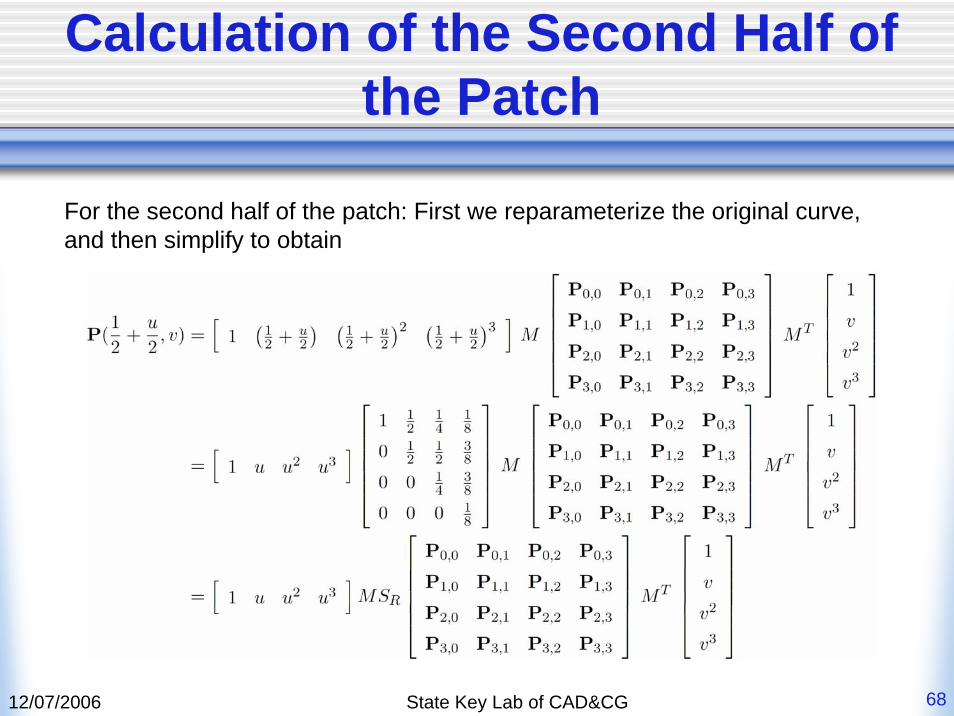
For the second half of the patch: First we reparameterize the original curve, and then simplify to obtain
12/07/2006 State Key Lab of CAD&CG 69
Calculation of the Second Half of the Patch
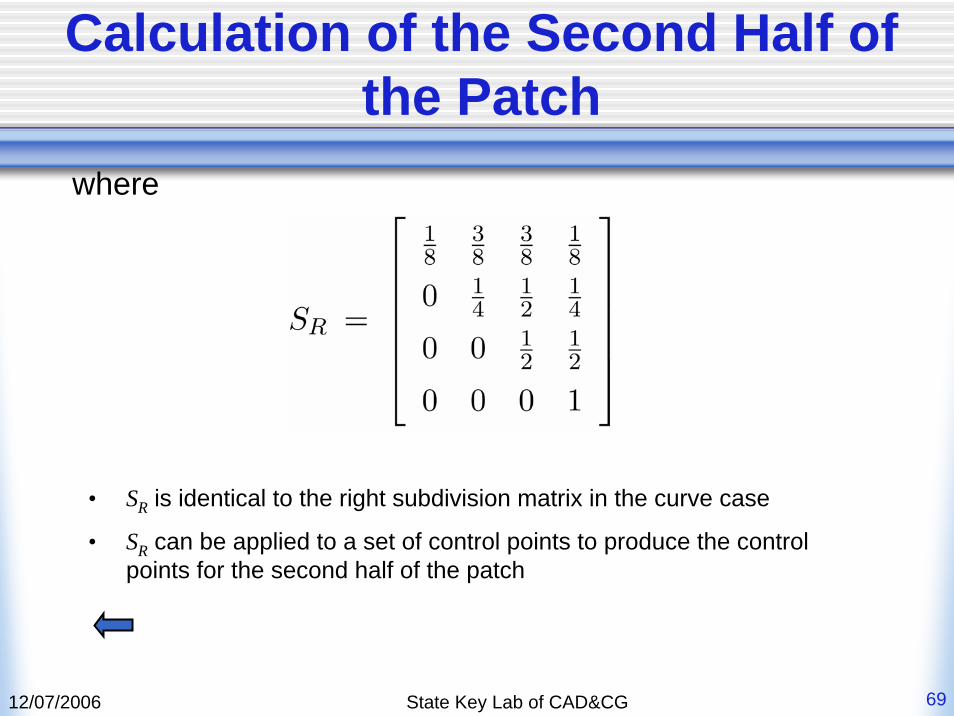
where
• SR is identical to the right subdivision matrix in the curve case
• SR can be applied to a set of control points to produce the controlpoints for the second half of the patch
12/07/2006 State Key Lab of CAD&CG 70
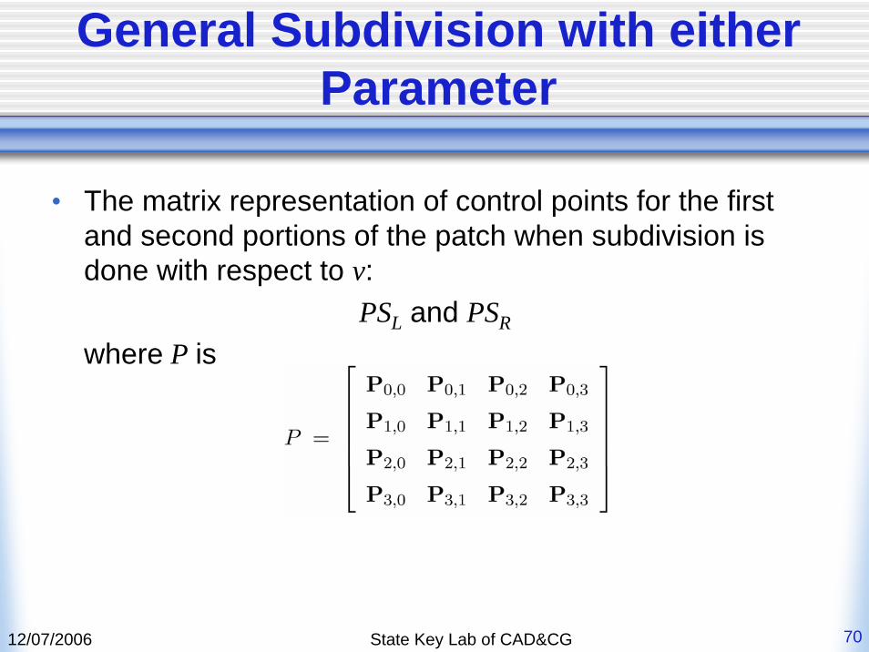
General Subdivision with either Parameter
• The matrix representation of control points for the first and second portions of the patch when subdivision is done with respect to v:
PSL and PSR
where P is
12/07/2006 State Key Lab of CAD&CG 71
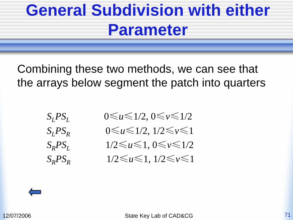
General Subdivision with either Parameter
Combining these two methods, we can see that the arrays below segment the patch into quarters
SLPSL 0≤u≤1/2, 0≤v≤1/2SLPSR 0≤u≤1/2, 1/2≤v≤1SRPSL 1/2≤u≤1, 0≤v≤1/2SRPSR 1/2≤u≤1, 1/2≤v≤1
12/07/2006 State Key Lab of CAD&CG 72
Advanced Topics on BézierCurves/Patches
• Triangular Bézier Patches • Rational Bézier Curves/Surfaces• Topics on Bézier
Degree ElevationDegree ReductionThe Variation Diminishing PropertyNonparametric Curves/Surfaces: (t,f(t))=(t(u), f(u))IntegralsGeometric ContinuityConversion between Different Bézier PatchesOffset ……

12/07/2006 State Key Lab of CAD&CG 73
Course Downloaded
http://www.cad.zju.edu.cn/home/jqfeng/GM/GM03.zip