An analytical pricing framework for financial assets with

An analytical pricing framework for financial assets

with trading suspensions

Lorenzo Torricelli∗

Christian Fries†

September 7, 2018

Abstract

In this paper we propose a derivative valuation framework based on Levy pro-

cesses which takes into account the possibility that the underlying asset is subject

to information-related trading halts/suspensions. For such assets are not traded at

all times, we argue that the natural underlying for derivative risk-neutral valuation

is not the asset itself, but a forward-type contract that when the asset is suspended

at maturity cash-settles the last quoted price plus the interests accrued since the

last quote update.elements of potential theory, we devise martingale dynamics and

no-arbitrage relations for such a forward process, provide Fourier transform-based

pricing formulae for derivatives, and study the asymptotic behavior of the obtained

formulae as a function of the halt parameters. The volatility surface analysis re-

veals that the short term skew of models with suspensions is typically steeper than

that of the underlying Levy models, indicating that the presence of a trade sus-

pension risk is consistent with the well-documented stylized fact of volatility skew

persistence/explosion.

Keywords: Market halts and suspensions, time changes, Levy subordinators, derivative

pricing, Levy processes.

MSC 2010 classification: 91G20, 60H99.

JEL classification: C65, G13.

∗Department of Mathematics, Ludwig Maximilians Universitat. Email: [email protected].†Department of Mathematics, Ludwig Maximilians Universitat. Email: [email protected].

1

mailto:[email protected]

mailto:[email protected]

L. Torricelli, C. Fries

1 Introduction

Suspending or halting1 of a stock from trading is a temporary emergency measure taking

place in event of abnormal market situations.

Broadly speaking this action is generally triggered by two distinct types of circum-

stances. The first is the manifestation of severe market anomalies that may prevent the for-

mation of a reliable price (e.g. crashes, order imbalance, excessive bid ask spread/illiquidity

holding back buyers). The second is the arrival of news that could have potential high

impact on the individual companies quotes. We can thus distinguish between endogenous

suspensions, generated by the market activity itself, and exogenous, news-related ones,

typically independent from day-to-day trading. Trade generated halts tend to be of fixed

time and short-lived, on the order of magnitude of minutes, whereas news-related suspen-

sion might last up to hours or days; their duration is typically discretionary. In case of

impactful business news arrival, the firm might file in for a trading suspension voluntarily,

e.g. motivated by internal management decision, or the action might be directly enforced

by the market authority, when there are growing concerns on the ability of the firm of

meeting the markets standards. In any case the purpose of a stock suspension, is to give

to all of the investors the opportunity to re-assess their positions, facilitate the issuance

of a better equilibrium price and reduce market information asymmetries.

Trade suspensions can, an do, occur quite often. Engelen and Kabir [8] observe that

in the years between 1992 and 2000 in the EuroNext stock market there were 210 pure

information related suspensions, 30% of which lasted more than one trading day, and

involved a total of 112 companies whose 49% was halted more than once. Christie et al.

[4] study a collective sample of 714 halts in the years 1997-1998 on the NASDAQ. Trading

suspensions then appear to be a market-wise repeatable process, of possibly inter-daily

duration.

The financial literature surrounding market halts, mainly focuses on whether the mar-

ket suspension do have the stabilizing effect on trade they are expected to deliver. The

evidence is mixed to some extent. Greenwald and Stein [10] suggest that halts facili-

tate formation of an equilibrium price by reducing transactional risk, whereas statistical

analyses in the NYSE and other US stock markets Corwin and Lipson [6], Lee et al. [16]

point to an increase in both post-halt trade volume and volatility, at odds with what

suspensions are meant to achieve.

However, typically these analyses include suspensions caused by order imbalances,

or triggering of the so-called circuit breakers due to some financial variable (especially

1Depending on the stock markets, halts and suspensions might have slightly different meanings. In

this article the two expressions are synonyms.

2

A pricing framework for assets with suspensions

volatility) breaching a safety threshold, which are market-generated events. Indeed, once

halts from order imbalances are removed from the sample, or only inter-daily suspensions

are considered, the general findings Christie et al. [4], Engelen and Kabir [8] is that when

the suspension last for more than one day the volatility of a stock is not sensibly impacted

by the halt.

To our knowledge, to date no research has been put forward to explore the impact of

suspensions/halts of stocks on prices of the possible derivatives written on such stocks. In

this paper we aim at providing a no-arbitrage pricing frameworks in markets with news

related trading halts. Since for derivative pricing the minimum horizon is daily, we do

not consider intra-daily stoppages due to circuit breakers or transactional frictions, under

the assumption that the changes in trading patterns these might determine are transient,

and do not extend to inter-daily trading.

Of course, halts might not produce any significant effect on valuations in the case the

expected suspensions are very short lived and maturity is long. However, the effect of a

suspension lasting for several days to several hours cannot be ignored altogether in certain

cases e.g. for pricing weekly options, a product that has recently drawn much attention.

One difficulty in introducing suspensions in no-arbitrage valuation may be that a secu-

rity that can be halted cannot be used as an underlying for martingale pricing. However

paradoxical this might sound, by definition, suspendable assets are not traded at all times,

and thus the replication/superreplication arguments establishing the equivalence between

no-arbitrage and martingale dynamics of the underlying do not in principle apply.

On the other hand referring to the physical suspendable market quote process is equally

problematic. Market prices that repeatedly halt cannot be made to drift to a continuous

constant rate after a measure change. A price quote that is subject to halts must preserve

the property of the paths being constant during suspension intervals, and therefore the

process cannot continuously drift at a risk-free rate after an equivalent measure change. To

borrow from the popular rule of thumb: “path properties do not change upon equivalent

measure changes”.

In the present paper we propose a solution to the conundrum above. We present a

continuous-time semimartingale model based on time-changed Levy processes that ac-

counts for trading halts in the underlying stock. Firstly, we inroduce a model for the

fundamental price of the stock recognizing that the evolution of the economic value might

follow different dynamics when the asset can be traded or it is suspended. Then we devise

an observable last market quote price process Qt by using a locally constant time change.

What we argue is that the natural underlying for derivative valuation on a suspendable

stock is a secondary forward process Ft that delivers at t the last observed quote Qt plus

3


the accrued interest since the last update of Qt. This contract has all the characteristics

we need: it can always be traded and exhibits martingale dynamics after an appropriate

equivalent measure change. In the legal stipulation of an over the counter derivative, Ft

effectively represents the real underlying asset if we consider the contract as referencing

the last market quote plus the interest rate payment.

From a methodological viewpoint, the framework introduces the idea of using a lo-

cally constant time change in option prices, obtained an inverse Levy subordinated time

change. Time changes in option prices are a well-established technique, (see e.g. Geman

et al. [9] but the literature is immense) that normally is used to capture the evolution

of the business activity. Our approach is rather different: our random time change is

a continuous, piece-wise linear time evolution whose paths can be constant at random

times. Those time intervals represent the trade halts. However, this is not yet sufficient:

in order to consistently model a market quote that undergoes halting we must further

introduce a second time change representing the last observable traded price of the stock

and generating the trade reopening asset price jump. The time change achieving this is

the so-called last sojourn process of a subordinator.

We devise no-arbitrage relations for the model by identifying a set of martingale mea-

sures under which both the asset St and the forward contract Ft are martingales. Adding

a suspension process to a pricing Levy model enriches its class of equivalent martingale

measures. In other words, the intrinsic market incompleteness of these new models also

accounts for an additional source of unhedgeable risk, the trading suspension risk, whose

market price is embedded in the risk neutral parameters of the Levy subordinator gener-

ating the halts.

Remarkably, the whole framework produces closed form formulae for the characteristic

function of Ft. This means that the well-established machinery of Fourier pricing (e.g.

Lewis [17]) is available, producing efficient option pricing algorithms.

Finally we consider the potential applications to the volatility surface modelling. Our

numerical experiments show a volatility skew which is at the same time much steeper

on the short term section and declines more slowly than that of the underlying Levy

models, thus generating a volatility term structure better matching the one observed in

the markets.

In Section 2 we discuss equity derivatives with suspensions and outline the economic

foundations of the framework. In Section 3 we introduce the stochastic model for the

fundamental price of the stock. In Section 4 we define the market quote process and the

traded underlying for derivative valuation; Section 5 deals with the equivalent martingale

relations for the model. Section 6 is dedicated to the identification of a pricing formula

4


and its convergence to prices from Levy models. Finally, in Section 7 we perform some

numerical tests for the pricing formula and analyze the arising volatility surfaces; com-

parisons with the pure Levy models are drawn. Some concluding remarks are expressed

in Section 8.

2 Derivatives on suspendable assets

The starting point for a valuation theory for stocks that undergo halts, is recognizing

that the classic theory of no-arbitrage pricing cannot be directly applied. Indeed, the

Fundamental Theorem (e.g. Delbaen and Schachermyer [7]) requires that the asset can

be traded at any time in order to form hedge and superhedge portfolios, which is not

the case when halts are present. Therefore, direct mathematical modelling of the market

asset seems not to be the correct way of addressing the problem.

We are thus faced from the very beginning with the problem of manufacturing some

form of syanthetic underlying which can be traded at any time regardless of possible

interruptions of the market activity, so that we can proceed in the usual vein within the

theory of no-arbitrage pricing.

Let us denote by Qt the stochastic process giving at time t the last available market

quote for the suspendable equity. Let τT the last instant prior to T where the equity was

last traded2 and

FX(t, T )t = er(T−t)Xt (2.1)

the forward value relative to the market traded asset Xt. Denote with r > 0 the prevailing

constant risk-free rate. The value of such a contract at time t, τt ≤ t ≤ T is

Ft := FQ(τt, t) = er(t−τt)Qτt = er(t−τt)Qt (2.2)

because by definition Qt = Qτt . One can thus consider the security Ft defined by (2.2),

promising the cash-settlement at time t of the last available asset market quote Qτt plus

the risk-free interest accrual (if any) from time τt until t. Conditional on time τt, Ft is the

value of a standard forward contract entered at τt and expiring at t on a traded underlying,

and as such is a well-defined security traded at all times, with a legally binding effective

date t and verifiable initiation date τt.

In this paper we propose using Ft as an underlying asset for derivative valuation on

stocks whose trade can be interrupted. This mathematical modelling idea reconnects

2Clearly most of the times τT = T but it is precisely when this does not happen that the discussion

is significant.

5


with the financial practice precisely because of equation (2.2). Indeed, a satisfactory

legal definition of an OTC derivative on a suspendable market asset requires an explicit

contractual specification of the actions to be undertaken when the market is closed at

maturity, because in such a case a current reference market value will not be available.

The most natural choice, and the one put in place for exchange-traded options, is using

as a reference value the last quoted price Qt of the underlying. The value to be used

for calculation of the payoff would thus be the last market quote Qt recorded prior to

the expiration time T . However, this seems to be unsatisfactory for at least two reasons.

Firstly, it completely ignores the time value of money, i.e. the growth of the fundamental

value of the asset during suspensions due to the interest rate component. Secondly using

Qt is not fully compliant of the risk-neutral valuation principles, as Qt is not a traded

instrument. Effectively, in view of (2.2), considering the risk-free interest rate accrual

when determining the payoff corrects at the same time both of these issues, and as we

shall show in this paper, allows for a full analytical derivatvie valuation framework.

Clearly, when interest rates are zero, Qt = Ft and in this special case the quote process

can indeed be used as a derivative underlying. However what we will show in this paper

is that for positive rates, and under some economic assumptions, it is Ft, and not Qt, to

possess martingale dynamics under some pricing measure. This result, together with the

previous remarks, seems to implicate that the market practice of using the last available

quote Qt for payoff calculation might be questionable from the theoretical perspective, at

least whenever rates are high or suspensions are long-lived, that is, when the difference

in valuation between calculating and not calculating interest accrual during the final

suspension is significant.

The starting element of our framework is an observable process St modelling the

fundamental (or intrinsic, or economic) stock value, which is distinct from its market

quote Qt. We emphasize again that neither of these two processes are traded assets. The

main idea is that the two must be coincide when the asset is tradable and may (will) differ

otherwise. When the asset is not traded, Qt is constant but St still evolves to keep track

of the economic activity surrounding the real asset. This assumption is naturally rooted

in the Efficiency Principle: when an asset can be traded all the available information are

reflected in its market quote. The process St is modelled by a two factors process; one

factor representing the price component purely due to trade, and another one the impact

on price of business and markets news and experts valuations. Only the first component

is halted during the market suspensions. Our models thus captures the existence of a

background noise of business-related information whose contribution to price formation

is distinct to that generated purely by the trading activity, and which persists also during

6


trading halts.

The following two sections are devoted to the identification of a rigorous mathematical

model for Qt and St. Once this is done, the considerations expressed in this section will

pave the way for a valuation theory for derivatives on suspendable stocks.

3 Fundamental value dynamics

In this section we begin structuring the fundamental value of the market stock St. We

consider a market filtration (Ω,Ft,F∞,P) satisfying the usual conditions and supporting

Levy processes and a money market account process paying a constant rate r > 0.

For a cadlag one-dimensional Levy process Yt with Levy triplet (µY , σY , νY (dx)) and

z ∈ U ⊆ C, for the characteristic function of Yt we use the notation:

E[e−izYt ] = e−tψY (z) (3.1)

where

ψY (z) = izµY +z2σ2

Y

2−∫R(e−izx − 1 + izx1I|x|<1)νY (dx) (3.2)

is the Fourier characteristic exponent of Yt. We denote the process of the left limits (the

“predictable projection”) of Yt with Yt−. By stochastic continuity, for all fixed t > 0 we

have Yt = Yt− almost surely. We write ∆Yt := Yt− Yt− for the process of the jumps of Yt.

As basic building blocks of our model we consider two one-dimensional indepen-

dent Levy processes Xt and Rt, with corresponding Levy triplets (µX , σX , νX(dx)) and

(µR, σR, νR(dx)) and characteristic exponents ψX and ψR. We also hasten to add the

standard conditions: ∫|x|>1

e2xνX(dx) <∞,∫|x|>1

e2xνR(dx) <∞ (3.3)

which are necessary for exponential Levy models to be square-integrable.

The process Xt and Rt retain the following financial interpretations. The evolution

of Xt represents the component of the log-asset price coming purely from the execution

of trades. The process Rt (the “rumor” process) instead models all of the other external

factors that may impact the price, mostly the dissemination of external news, both fi-

nancial and non-financial. Normally Xt is expected to dominate Rt, but it does not have

to be so. When trading for the asset is allowed, the stock returns are defined to be the

independent sum of these two factors. However, as explained in the previous seciton, we

7


shall require that as a trade halt occurs, Xt does not evolve, while Rt still contributes to

the fundamental price formation.

Let us introduce the generator of the market suspensions as a compound Poisson

process Gt independent of (Xt, Rt), of the following form:

Gt = t+Nt∑i=0

ξi (3.4)

with the variables ξi being independent identically exponentially distributed of common

rate parameter β, and Nt is a Poisson process of intensity λ independent of the ξis and

all the remaining processes.

For s ≥ 0 the Laplace characteristic exponent φG(s) of Gt satisfies

E[e−sGt ] = e−tφG(s) (3.5)

and is given by

φG(s) = s+

∫R+

(1− e−su

)νG(du) =

λs

s+ β+ s. (3.6)

Finally we introduce the market suspensions process Ht as the “inverse” of Gt. More

precisely, for all t we define Ht as the first exit time of the level t of Gt, that is:

Ht = inf s > 0 |Gs > t . (3.7)

When Gt jumps, Ht has a flat spot, and a market suspension occurs. Furthermore the

duration of the suspension is exactly given by the size of the jump. In the instants between

the jumps of Gt, Ht is just the linear calendar time. In other words, we have the following

definition:

Definition 3.1. Let R be the image of Gt. We say that St is suspended, halted or non-

tradable at t > 0 if t ∈ Rc. If s > 0 is such that Gs− 6= Gs then ∆Gs is the duration of

the halt.

It is important to notice that taht Ht ≤ Gt and the equivalence Ht ≤ s = Gs ≥ t,which in particular yields Ht ≤ t = Ω. Since Gt is strictly increasing, Ht is continuous,

and it is a stopping time for all fixed t. Also, Ht is almost surely increasing, bounded

almost surely, and limt→∞Ht =∞ almost surely, and thus it is a valid time change (Jacod

[11], Chapter 10).

We are now in the position of describing the fundamental economic value of our sus-

pendable asset St. Upon suspension the evolution of the asset value should instead be

fully determined by the news arrival. The fundamental price St is thus defined as follows:

St := S0 exp(XHt +Rt), S0 > 0. (3.8)

8


The writing XHt indicates the time-changed semimartingale process in the sense of

Jacod [11]. Since Ht is continuous, Xt is Ht-continuous3. This means that XHt retains

many of the good properties of Xt (again, Jacod [11], Chapter 10); in particular it is an

FHt-adapted semimartingale. Finally, recalling that A ∈ FHt if and only if A ∩ Ht ≤s ∈ Fs for all s, choosing s = t and observing Ht ≤ t = Ω shows FHt ⊂ Ft, so that St

is also an Ft-adapted semimartingale.

The fundamental price evolution St has the property we were striving for. Condition-

ally on the asset being tradable, i.e. Gt not jumping, we have that XHt+Rt = Xt+Rt and

the price process is jointly determined by the economic reaction to trade and an external

news flow. When Gt jumps, the stochastic time Ht and thus the price component XHt

are constant, and the fundamental price is driven only by the news dissemination process

Rt.

Finally, we associate to St the corresponding Levy exponential model S0t without halts,

whose dynamics are given by

S0t := S0 exp(Xt +Rt). (3.9)

Further on, we shall be interested in comparing financial valuations relying on St with

the analogous on its pure Levy counterpart S0t , in order to assess the impact of the

introduction of trading halt periods in derivative pricing.

4 The asset quote process and the traded underlying

We must at this point rigorously define the quote process Qt recording the last available

market quote of St at time t. Recall that R is the range of Gt.

The last sojourn process of Gt of the level [0, t] is defined as:

τt = sups < t, s ∈ R ≤ t (4.1)

This process keeps track of the last position of Gt in all the level sets, and for all fixed

t we will interpret as a random time. Indeed, as t varies, this process can be regarded as

a time change. We have the following result (see also Bertoin [1], Section 1.4):

Lemma 4.1. The process τt satisfies

τt = GHt− (4.2)

and there exists a right-continuous modification of τt which is an Ft-time change .3A process Yt is said to be continuous with respect to a time-change Tt if it is almost surely constant

on the sets [Tt−, Tt].

9


Proof. As Gt− is adapted to Ft the process GHt− is adapted to FHt but since FHt ⊂ Ftthen it is also Ft-adapted and thus GHt− is an Ft-stopping times for all t.

To show (4.2) observe that for all s we have:

GHt− > Gs = Ht > s = Gs < t, (4.3)

so that GHt− ≥ τt almost surely. But since GHt− ≤ t surely, then the equality holds.

Therefore, being τt increasing and almost surely finite it is a time changes when looked

at as aprocess if a right-continuous modification exists. This is attained by replacing τt

with τt+ in the almost-surely null Lebesgue measure set where τt is discontinuous, and

that the new process is a modification is granted by stochastic continuity.

From now on we will make use of the right-continuous version of τt. It is crucial to

observe from the definitions above that τt < t if and only if t ∈ Rc, i.e. according to

Definition 3.1 if and only if the asset is suspended at t; conversely, τt = t if and only if

the asset is traded at t. We therefore denominate τt the last market quote time process.

Observe that τt has a jump discontinuity exactly at the market reopening times given by

t = Gs, ∆Gs 6= 0, i.e. the points in R isolated on their left.

To see the importance of τt we begin by showing that using this process we can

calculate the probability of the asset being tradable at any given time t.

Proposition 4.2. We have that

P(τt = t) =β + λe−(λ+β)t

β + λ(4.4)

for all t > 0.

Proof. We recall that the q-th potential measure U q(dx) of a Levy process Lt is defined

as the occupation measure

U q(dx) =

∫ ∞0

e−qtP(Lt ∈ dx)dt. (4.5)

If U q(dx) is absolutely continuous, its Radon derivative uq(x) is called the potential den-

sity. When q = 0 and Lt is a subordinator U0(dx) and u0(x) also go under the name of

renewal measure (resp. density). In this case we drop the superscript and write U(dx)

and u(x).

By Theorem 5 in (Bertoin [2], Chapter 3) we have that since Gt has drift d = 1, its

renewal density exists, can be chosen continuous, and satisfies P(Tt = t) = u(t) where

10


Tt = GHt is the first sojourn of Gt of [t,∞). Now observe that the well-known relationship

(e.g. Bertoin [1], Section 1.3)

L(U(dt), s) =

∫ ∞0

e−stu(t)dt =1

φG(s)(4.6)

yields

L(U(dt), s) =1

s

β + s

β + λ+ s. (4.7)

On the other and, by a direct calculation∫ ∞0

e−stβ + λe−(λ+β)t

λ+ βdt =

1

s

β

β + λ+

λ

β + λ

1

λ+ β + s=

1

s

β + s

β + λ+ s. (4.8)

The uniqueness of the Laplace transform for continuous functions then yields

P(Tt = t) =β + λe−(λ+β)t

λ+ β(4.9)

To conclude, observe that by (Bertoin [2], Chapter 3, Proposition 2.ii) we know that

P(τt < t, Tt = t) = 0 for all fixed t entailing P(τt = t|Tt = t) = 1. Also, P(τt = t, Tt >t) = P(∆Gt 6= 0) = 0 because a Levy process is stochastically continuous, so that also

P(Tt = t|τt = t) = 1. By conditioning the event τt = t, Tt = t one then sees that

P(Tt = t) = P(τt = t) so that (4.4) follows in view of (4.9).

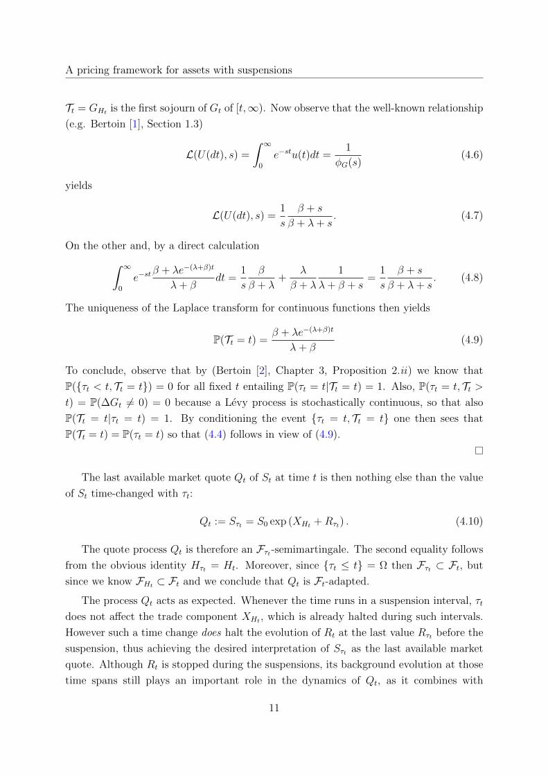
The last available market quote Qt of St at time t is then nothing else than the value

of St time-changed with τt:

Qt := Sτt = S0 exp (XHt +Rτt) . (4.10)

The quote process Qt is therefore an Fτt-semimartingale. The second equality follows

from the obvious identity Hτt = Ht. Moreover, since τt ≤ t = Ω then Fτt ⊂ Ft, but

since we know FHt ⊂ Ft and we conclude that Qt is Ft-adapted.

The process Qt acts as expected. Whenever the time runs in a suspension interval, τt

does not affect the trade component XHt , which is already halted during such intervals.

However such a time change does halt the evolution of Rt at the last value Rτt before the

suspension, thus achieving the desired interpretation of Sτt as the last available market

quote. Although Rt is stopped during the suspensions, its background evolution at those

time spans still plays an important role in the dynamics of Qt, as it combines with

11


the discontinuities of τt to determine the “jump” in the reopening price4. Outside the

suspension intervals we have the plain relation τt = t.

Now, according to Section 2, the traded underlying to be used for derivative valuation

is the process Ft in (2.2). Observe that this process is Ft-adapted. Now let f be a

square-integrable contingent claim maturing at T . The value V0 of f on Ft is given by

V0 = EQ[e−rTf(FT )] (4.11)

where Q is a P-equivalent (local) martingale measure under which the discounted process

e−rtFt is a martingale. Now, observe that:

e−rtFt = e−rτtQt. (4.12)

Therefore we have the derived following no-arbitrage principle for suspendable stocks.

No-arbitrage principle for securities with market suspensions. In the model il-

lustrated, the martingale property of the discounted forward value Ft is equivalent to the

martingale property of the quote process Qt discounted with the stochastic discount factor

e−rτt.

In the next section we explore the implications of this principle for the determination

of equivalent martingale measure/no-arbitrage relations for option pricing on financial

securities with market halts. Before moving on, let us briefly summarize the framework.

Construction of an underlying traded security when securities can be suspended:

1. Select processes Xt and Rt for the market trade and rumor price components, as

well as a specification of the market halt generating process Gt;

2. introduce the fundamental value St of an asset with market halts as in (3.8);

3. determine the quote process Qt by time changing St with the last price observation

time τt prior to t;

4. define the traded forward contract Ft delivering the cash amount Qτt in t, whose

value in t is Ft = er(t−τt)Qt.

4Strictly speaking also Xt determines the new opening price, but Rt cumulates variation during the

suspension intervals, whereas Xt just affects the price through XHtwhich in turn - by construction - only

releases instantaneous variability at reopening. Thus its contribution to the variance is much inferior.

12


Using a common drawing from Xt, Rt and Gt we visualize the processes Gt, Ht, St, τt,

Qt and Ft in Figures 1 to 4. We have used S0 = 100, µX = 0.3, σX = 0.5, µR = −0.2,

σR = 0.2 and νX = νR = 0, so that conditional on being traded the asset follows the

Black-Scholes-Samuelson model with drift µ = 0.1 and volatility coefficient σ = 0.5385.

The asset halt parameters are λ = 1 and β = 7.

5 Risk neutral dynamics and price of trade suspen-

sion risk

We now proceed to investigate the martingale dynamics of the discounted asset e−rtFt.

In view of the no-arbitrage principle, this is equivalent to determine the no-arbitrage

dynamics of the stochastically-discounted quote price e−rτtQt. As we shall see, because

of the boundedness of τt, to achieve this is sufficient to determine martingale relations on

the fundamental price St.

To make the discussion more transparent, we introduce the following general propo-

sition, stating that under certain conditions time change and measure change commute.

For general background see Jacod and Shiryaev [12], Jacod [11] and Kallsen and Shiryaev

[13].

Lemma 5.1. Let Xt be a semimartingale on a filtered space (Ω,P,F ,Ft) which is con-

tinuous with respect to a time change Tt and Zt a martingale density process having the

stochastic exponential representation:

Zt = E(∫ t

0

HudXcu +

∫ t

0

(W (u, x)− 1)(µX − νX)(dx× du)

)(5.1)

where Xct is the continuous martingale part of Xt, µ

X and νX respectively its jump measure

and jump compensator, Ht some square-integrable process integrable with respect to Xct ,

and W (t, x) a random function such that the second integral in (5.1) exists. The symbol

E(·) stands for the stochastic exponential.

Assume further that ZTt is a true martingale, and denote by Q and QT the P-equivalent

martingale measures associated respectively with Zt and ZTt. We have:

(XTt)QT = XQ

Tt. (5.2)

Proof. Let (µt, σt, ν(dt × dx)) be the P-characteristics of Xt. By the Girsanov Theorem

for semimartingales (Jacod and Shiryaev [12], Chapter III, Theorem 3.24) their Q coun-

terparts, in the “disintegrated” (Jacod and Shiryaev [12], Chapter II, Proposition 2.9)

13


form are

µQt = µt +

∫ t

0

HuσudAu +

∫|x|<1

(W (t, x)− 1)Kt(dx) (5.3)

σQt = σt (5.4)

νQ(dt× dx) = dAtW (t, x)Kt(dx) (5.5)

for some predictable process At and random measure Kt(dx). Furthermore, according to

(Jacod and Shiryaev [12], Lemma 2.7), by the adaptedness of Xt to Tt the characteristics

of XTt under Q are (µTt , σTt , ν(dTt× dx)). Now by (Jacod 11, Theorems 10.19, 10.27) we

have that:

ZTt = E(∫ t

0

HTudXcTu +

∫ t

0

W (Tu, x)(µX − νX)(dx× dTu)). (5.6)

Therefore by applying the Girsanov’s Theorem to XTt with respect to the density ZTt we

obtain, taking into account 〈∫ ·

0HTudX

cTu〉t =

∫ Tt0HuσudAu (because of Jacod 11, Theorem

10.17), the following characteristics:

µQTt = µTt +

∫ Tt

0

HuσudAu +

∫|x|<1

(W (Tt, x)− 1)KTt(dx) (5.7)

σQTt = σTt (5.8)

νQT

(dt× dx) = dATtW (Tt, x)KTt(dx) (5.9)

which match (µQTt, σQ

Tt, νQ(dTt × dx)).

We can then directly state the main result of this section, on the martingale relations

for the fundamental asset price process.

Theorem 5.2. Let St be given by (3.8). Under mild assumptions on Xt and Rt, there

exists a set of equivalent martingale measures QX,R,H with Radon-Nikodym of the form

dQX,R,H

dP= XtRtHt (5.10)

for some density processes Xt and Rt, and

Ht = exp

((λ− λ∗)t+

∑s≤t

(β∗ − β)∆Gs

)(5.11)

such that under QX,R,H the discounted fundamental price process e−rtSt is an FHt-martingale

of the form exp(X∗H∗t

+R∗t −rt) for some Levy processes X∗t , R∗t and H∗t a compound Pois-

son process of drift one, intensity λ∗ and exponentially i.i.d. jumps of rate β∗.

14


Proof. Under the equivalent martingale measure induced by Ht, we have that the dy-

namics of Gt are those of a compound Poisson process with intensity λ∗ and exponential

jump distribution of parameter β∗ (e.g. Sato 19, Theorem 33.1). We denote by H∗t the

dynamics of Ht under the P-equivalent measure induced by Ht.

The first step is to isolate a change of measure under which exp(Xt) and exp(Rt) are

individually martingales. By standard arguments (the Esscher transformation, e.g. Cont

and Tankov 5, Proposition 9.9), so long as Rt and Xt are not themselves subordinators,

it is possible to find martingale density processes Rt and X 0t under which Rt and Xt are

Levy processes of triplets respectively (µ0X , σX , ν

0X(dx)) and (µ∗R, σ

∗R, ν

∗R(dx)) where:

µ0X = −(σ0

X)2/2−∫R(ex − 1− x1I|x|<1)ν0

X(dx) (5.12)

σ0X = σX (5.13)

dν0X

dνX= exp(Φ0) (5.14)

and

µ∗R = −(σ∗R)2/2−∫R(ex − 1− x1I|x|<1)ν∗R(dx) + r (5.15)

σ∗R = σR (5.16)

dν∗RdνR

= exp(Φ∗) (5.17)

for functions Φ∗ and Φ0 satisfying certain integrability conditions.

After having operated the P-equivalent change of measure corresponding to Ht, we

set Xt = X 0H∗t. Since X 0

t is a martingale and H∗t a bounded stopping time, by Doob’s

Optional Sampling Theorem, Xt is also a martingale. Furthermore X 0t has the exponential

representation (5.1), and so by Lemma 5.1, under the equivalent measure induced by XtRt

we calculate the characteristics (µ∗X(t), σ∗X(t), ν∗X(dx× dt)) of the semimartingale XH∗t

in

the measure induced by XtHt by simply time changing (5.12)-(5.14), yielding:

µ∗X(t) = −H∗t (σ0X)2/2−H∗t

∫R(ex − 1− x1I|x|<1)ν0

X(dx) (5.18)

σ∗X(t) = σXH∗t (5.19)

ν∗X(dx× dt) = dH∗t ν0X(dx). (5.20)

Recall that the (Fourier) cumulant process KXt (θ) of a quasi-left continuous semi-

martingale Xt with finite first exponential moment is the almost-surely uniquely deter-

mined processKXt (θ) such that in the appropriate domains of definition exp(iθXt−KX

t (θ))

15


is a local martingale. In the case of a Levy process, in our notation KXt (θ) = −tψX(−θ).

By Kallsen and Shiryaev [13], Lemma 2.7, one has that if Tt is a time change and Xt is

Tt-continuous KXTt (θ) = KX

Tt(θ).

But then observe that XHt and Rt under the measure QX,R,H induced by XtRtHt have

dynamics respectively X∗H∗t

= XH∗t−KX

H∗t(−i) and R∗t = R∗t −KR

t (−i) + rt, with XH∗t

and

R∗t being the driftless processes with characteristics given respectively by (0, σ∗X(t), ν∗X(dx×dt)) and (0, tσ∗R, ν

∗R(dx)dt). Therefore, by independence exp(X∗H∗

t+ R∗t − rt) is a local

martingale under QX,R,H , with exp(R∗t − rt) being a true martingale since R∗t is a Levy

process. Finally conditioning and using the independence of H∗t and X∗t yields that for all

t, E[exp(X∗H∗t)] = 1 so that exp(X∗H∗

T+ R∗t − rt) is indeed a martingale. This terminates

the proof.

Comparing to the corresponding results for Levy processes, the added complexity

here is operating the “measure change of a time change”, which may potentially affect

the martingale densities for the “spatial” components themselves. However, because of

the independence and time-change continuity relationships, the densities factor and this

is indeed not the case.

It is now a simple consequence of the structure of the discussion in Section 3 and

Theorem 5.2 that Ft is also a martingale under the measures QX,R,H .

Corollary 5.3. Let FHt = FHt. Under the measures QX,R,H in Proposition 5.2, Ft is an

FHτt -martingale.

Proof. By Proposition 5.2 we have that e−rtSt is an FHt -martingale under QX,H,R. But

since τt is a bounded stopping time, we can apply Doob’s Optimal Sampling Theorem

from which follows that e−rτtSτt = e−rτtQt = e−rtFt is an FHτt -martingale.

In the process of isolating the martingale density process corresponding to the change

of measure to the equivalent risk-neutral ones, we can appreciate that this model is in-

trinsically incomplete, and that pricing incorporates two sources of unhedgeable risk.

First, as in any model based on Levy processes, the presence of jumps in the drivers

Xt and Rt bears a source of systematic risk which cannot be completely hedged by trading

in a set of fundamental securities. Second, modelling the asset halts by a random time

change driven by a Levy subordinator introduces an additional source of market risk

which is equally unhedgeable in terms of replication. This risk correspond to the “totally

inaccessible” events of a suspension taking place. A suspension can happen at any time

without notice: suspension times are not predictable times. Hence derivatives on assets

with halts cannot be perfectly replicated using a predictable trading strategy.

16


Consequently, the introduction of a “horizontal jumpiness” of the securities brings

about the concept of market price of suspension risk embedded in the parameters λ∗ and

β∗. These parameters encode the premium that the investors should demand for holding

an investment which is subject to suspensions.

6 Contingent claim valuation

In order to obtain semi-closed pricing formulae we exploit the fact that since Xt and Rt

are independent of Gt, so they are of both τt and Ht. Combining this property with

the fact that we are effectively able to compute the joint Laplace-Laplace transform of

(Ht, τt), we can obtain pricing formulae applying the well-known Fourier techniques.

In this section, we use the ·∗ notation when we want to emphasize the risk neutral

dynamics or parameters of a process.

Let us begin from the derivation of the Laplace-Laplace transform of the joint density

of an inverse subordinator Ht and its last sojourn process GHt−.

Proposition 6.1. Let Gt be any strictly increasing subordinator and Ht is inverse as

defined as in (3.7), denote by Pt(x, y) the joint law of (Ht, GHt−) and let Pt(q, k) =

E[e−qHt−kGHt− ]. The Laplace transform in the variable t of Pt(q, k) satisfies:

L(Pt(q, k), s) =

∫ ∞0

e−stPt(q, k)dt =1

s

φG(s)

q + φG(k + s). (6.1)

Proof. Because of the possibility of an atom at t in GHt− we must divide

L(Pt(q, k), s) =

∫ ∞0

e−stE[e−qHt−kGHt−1IGHt−=t] +

∫ ∞0

e−stE[e−qHt−kGHt−1IGHt−<t].

(6.2)

It is shown in Kyprianou [14], Chapter 5, that if the drift d of Gt is positive

E[e−qHt1IGHt−=t] = duq(x) (6.3)

where uq(x) is the q-th potential measure of Gt (and such quantity is zero otherwise),

whence∫ ∞0

e−stE[e−qHt−kGHt−1IGHt−=t]dt =d

∫ ∞0

e−(s+k)tuq(x)dx

=d

∫ ∞0

e−(q+φG(k+s))tdx =d

q + φG(s+ k). (6.4)

17


Let us turn to study the transform of (Ht, GHt−) on the set GHt− < t. By conditioning

on Ht = x applying Fubini’s Theorem and writing f(x, t) for the density of Ht (which

exists by Meerschaert and Scheffler 18, Theorem 3.1):

E[e−qHt−kGHt−1IGHt−<t] =

∫ ∞0

e−qxf(x, t)dx

∫ t

0

e−kyP(GHt− ∈ dy|Ht = x)

=

∫ t

0

e−kydx

∫ ∞0

e−qxP(GHt− ∈ dy,Ht = x). (6.5)

The crucial remark is now that:

GHt− < y,Ht = x = Gx− < y,Gx ≥ t = Gx− < y,∆Gx > t−Gx−. (6.6)

Hence, define the point process:

γtx =∑s≤x≤t

1I∆Gs>t−Gs− (6.7)

and denote the tail density νG(u) = νG(u,∞). Since Gx has Levy measure νG, for a Borel

random set A the point process∑

s≤x 1I∆Gs∈A has compensating measure νG(A)dx, and

thus γtx has compensating measure νG(t−Gx−)dx. Therefore, as 1IGx−<y is predictable,

by virtue of (6.6), the compensation formula (e.g. Last and Brandt 15, Proposition 4.1.6)

Fubini’s Theorem and stochastic continuity of Gx we calculate:∫ ∞0

e−qxP(GHt− ≤ y,Ht = x)dx = E[∫ ∞

0

e−qx1IGx−<ydγtx

]= E

[∫ ∞0

e−qx1IGx−<yνG(t−Gx−)dx

]=

∫ ∞0

e−qxdx

∫ y

0

P(Gx ∈ dz)νG((t− z)−)

=

∫ y

0

U q(dz)νG(t− z). (6.8)

The last equality follows because U q has no atoms and the set of discontinuities of a Levy

measure has Lebesgue measure zero. Thus:

E[e−qHt−kGHt−1IGHt−<t] =

∫ t

0

e−kyU q(dy)νG(t− y)dy (6.9)

so that, again applying Fubini’s Theorem:∫ ∞0

e−stE[e−qHt−kGHt−1IGHt−<t]dt =

∫ ∞0

e−stdt

∫ t

0

e−kyU q(dy)νG(t− y)dy

=

∫ ∞0

∫ t

0

e−s(t−y)e−(k+s)yU q(dy)νG(t− y)dtdy

=L(νG(t), s)L(U q(dy), k + s). (6.10)

18


Using the formula (e.g. Bertoin 2, Section III.1)

L(νG(t), s) =φG(s)

s− d (6.11)

and the second and third equalities in equation (6.4) again (with d = 1), we obtain∫ ∞0

e−stE[e−qHt−kGHt−1IGHt−<t] =1

q + φG(s+ k)

(φG(s)

s− d)

(6.12)

and by substituting (6.12) and (6.4) in (6.2) the proof is complete.

This proposition extends Bertoin [1], Lemma 1.11, and is somewhat reminiscent of the

Wiener-Hopf factorisation formulae and analogous identities in Levy potential theory (see

Bertoin [2], Kyprianou [14]).

Now, the independence of the involved processes allows to transition from the Laplace-

Laplace transform of the time changes to the Laplace transform of the characteristic

function of the log-value for the traded underlying Ft. After a Laplace inversion, the

latter can be in turn used to derive an integral option price representation. The full result

reads as follows:

Theorem 6.2. Let f(x) be a contingent claim on logFt maturing at time T , assume that

w(x) = f(ex) is Fourier-integrable and let Sw be the domain of regularity of its Fourier

transform w(z). Denote with SF the domain of regularity of EQ[e−iz logFT ], and assume

Sw ∩ SF 6= ∅. The price V0 of the derivative paying off f(FT ) at time T is given by:

V0 = EQ[e−rTw(logFT )] =e−rT

2π

∫ iγ+∞

iγ−∞S−iz0 e−izrT w(z)ΦT

(ψ∗X(z), ψ∗R(z), λ∗, β∗

)dz

(6.13)

with

Φt

(z1, z2, λ, β

)= (Debt)−1·(

β2ct(dt − 1)(λ+ z2)− z2

(2ebtλa+ e(ctdt(a− λ− z1) + ct(λ+ z1 + a))

)+ βc((dt − 1)λ2

+ λ(z1 − dtz1 + a+ dt(a− z2) + z2) + z2(−2(dt − 1)z1 + a+ dt(a− z2) + z2)))

(6.14)

wherea =

√β2 + 2β(λ− z1) + (λ− z1)2

bt = exp(t2(z1 + 2z2 + λ+ a)

)ct = eβt/2

dt = eat

e = z1 + z2

D = 2a(β(λ+ z2)− z2(λ+ e))

(6.15)

19


and γ is chosen such that the integration contour lies in Sw ∩ SF .

Proof. Since Sw∩SF 6= ∅, by the discussion in Lewis [17], and conditioning under indepen-

dence, we have that the value V0 of a derivative can be represented as the Parseval-type

convolution:

V0 = e−rtEQ[w(log(FT ))] =e−rt

2π

∫ iγ+∞

iγ−∞EQ[e−iz logFT ]w(z)dz

=e−rt

2π

∫ iγ+∞

iγ−∞S−iz0 e−izrTEQ[e−ψ

∗X(z)HT−ψ∗

R(z)GHT− ]w(z)dz.

(6.16)

for some γ chosen in Sw ∩ SF . But then using Proposition 6.1 and taking the analytic

continuation on the convergence domain of the Laplace transform we have for some z1, z2 ∈C:∫ ∞

0

e−stEQ[e−z1HT−z2GHT− ]dt =1

s

φ∗G(s)

z1 + φ∗G(z2 + s)

=1

β∗ + s

(β∗ + λ∗ + s)(β∗ + sz2)

(z1 + z2 + s)(β∗ + z2 + s) + λ∗(s+ z2). (6.17)

By explicitly calculating the inverse Laplace transform of the last line of (6.17) with

MATHEMATICA we obtain equation (6.14)-(6.15).

We conclude this section by a natural result that guarantees, in line with the intuition,

that the prices of claims written on Ft should converge to those from the benchmark Levy

model without halts S0t , as the halt frequency and average duration tend to zero.

Proposition 6.3. Let f be a bounded claim maturing at T . We have the following

asymptotic relations for V0:

(i) If V 00 is the value of the claim f written on S0

t then:

limλ∗→0

V0 = limβ∗→∞

V0 = V 00 ; (6.18)

(ii) Let ξ an exponential independent time of parameter λ∗. For a stochastic process Yt

define

Y ξt =

Yt if t < ξ

Yξ, if t ≥ ξ.(6.19)

Then

limβ∗→0

V0 = V ξ0 (6.20)

where V ξ0 is the discounted expectation of f taken with respect to the distribution of

the terminal random variable SξT = S0 exp((X∗)ξT + (R∗)ξT ).

20


Proof. From Proposition 6.1 and using independence we see that in the risk-neutral mea-

sure

limλ∗→0

P (z, s) = limβ∗→∞

P (z, s) =1

ψ∗X(z) + ψ∗R(z) + s

=L(e−T (ψ∗X(z)+ψ∗

R(z)), s) = L(E[e−iz(X∗T+R∗

T )], s) (6.21)

Taking the limits inside the Laplace integral by dominated convergence and inverting the

transform we see by the Levy Continuity Theorem that ST tends in distribution to S0T for

the given parameter asymptotics. This completes the proof of (i).

For ξ as in (ii) define the killed linear drift

λ∞t =

t if t < ξ

∞, if t ≥ ξ(6.22)

whose De Finetti-Levy-Kincthine exponent is φλ(s) = λ∗ + s, and consider its first exit

time process

λt = infs > 0|λ∞s > t =

t if t < ξ

ξ, if t ≥ ξ(6.23)

Evidently λ∞λt− = λt, so we can apply Lemma 1.11 in Bertoin [1] for a subordinator with

killing directly to the process λt; note also that Sξt = Sλt . Taking the limit in Proposition

6.1 and using independence, shows that

limβ∗→0

P (z, s) =1

s

λ∗ + s

ψ∗X(z) + ψ∗R(z) + λ∗ + s

= L(E[e−(ψ∗X(z)+ψ∗

R(z))λT , s) = L(E[e−iz((X∗)ξT+(R∗)ξT )], s) (6.24)

and the result again follows again by interchanging integration and limit, inverting the

transform and applying Levy Continuity Theorem.

The first part of this proposition guarantees convergence of put prices on Ft to those of

the associated unhalted model S0t . Convergence of call prices then also holds by call-put

parity.

The second part has the interpretation that as the expected length of jumps tends to

infinity, the implied asset process tends to a price distribution with only one halt that

freezes the asset value at the last recorded price until maturity, and that for every possible

maturity. The risk-neutral distribution of the waiting time of such an halt is that of a

single Poisson event in Gt, that is, an exponential independent time of parameter λ∗.

In combination with Proposition 4.2, this result can be helpful to assess the relative

impact of the halts on prices, something we will pursue in the next section.

21


7 Numerical experiments

We begin by visualizing equation (4.4) to get a better idea of how the probabilities of

suspension, and therefore prices, depend on λ, β. In Figure 5 for a given time horizon

t = 0.5 we plot the probabilities as a function of λ and β. As λ→ 0 this probability tends

to 1 and the model converges to S0t . In Figure 6 instead we fixed λ = 1 and β = 10 and

as time increases the probability of t falling in a suspension decreases to its asymptotic

value β/(β + λ). This means that, everything else being equal, we expect the absolute

differences of prices compared to S0t to be higher for longer maturities.

For price generation we considered an instantiation of our model were Xt is the CGMY

model of Carr et al. [3] with one set of calibrated parameters found therein, namely:

C = 6.51, G = 18.75, M = 32.95, Y = 0.57. (7.1)

We choose Rt as a Brownian motion with µR = 0, σR = 0.2, and set a risk-free rate r = 2%

and S0 = 100. We take this parameter set as the baseline scenario.

We represent then prices corresponding to an at-the-money call option on Ft with same

maturity and same parameters λ∗ and β∗ of Figure 5. We can see that indeed Figure 7

closely mirrors Figure 5. As λ∗ → 0 and β∗ → ∞, in accordance to Proposition 6.3, the

prices converge to the line 11.883 given by the price in the associated Levy model S0t .

Also, note that this convergence is naturally increasing in both λ and β, since halting

the asset has the effect of compressing the volatility and thus lowering the price. As

the number of expected halts and their average duration go to zero, the variability of S0t

is restored and price convergence attained. In Figure 8 we represent the effect of this

lowering on theta. As one could expect, also in view of Figure 6, the option prices grow

slower as time to maturity increases.

In Figures 9 to 16 we compare some volatility skews extracted from options on S0t

and St. We want to show how acting on the halt parameters λ∗, β∗ and σ∗R, dictating

respectively the (risk-neutral) frequency and average duration of the halts, and the vari-

ance of the price quote jump at re-opening, fundamentally alters the skew structure of

the benchmark model S0t . We initially set as baseline λ∗ = 2 and β∗ = 50, corresponding

to a bi-yearly suspension frequency with an average length of five days.

Figure 9 shows the baseline scenario with monthly maturity. It can be noticed the

excess at-the-money steepness of the halted model compared to the Levy one, while the

two skews retain the same structure in and out of the money. As we shorten the maturity

to bi-weekly, this difference gets lost, as can be seen in Figure 10: the likelihood of a halt

22


λ∗t is too small for the given parameters β∗ and σ∗R to generate any noticeable difference

of the implied price distributions from those of S0t .

Therefore, in the bi-weekly maturity case we change σ∗R to σ∗R = 0.5 and hold the other

parameters constant. We can see in Figure 11 that the resulting increase in the variance

of the reopening price shocks is enough to recreate the excess at-the-money skew already

observed in Figure 9. Of course, with this modification the one-month skew difference is

exacerbated (Figure 12).

Analogously we proceed to alter λ∗ and β∗. Fixing the maturity to monthly and all the

remaining parameters to the baseline case, we first change λ∗ = 12 (suspensions expected

with monthly frequency) and then β∗ = 12 (monthly expected suspension length). The

resulting Figures 13 and 14 show similar effects on the skew that the one attained in

Figure 11 by chagning σ∗R. Note also that associated to this parameter change is also a

minimal lowering of the level of the skew, consistently with the discussed effect that a

decrease in β∗ and an increase in λ∗ determine a global reduction of the option prices.

Last but not least, we find the effect on the skew for λ∗ and β∗ to be persistent in

time. In Figures 15 and 16 the same situation of Figures 13 and 14 is reproduced, but this

time with maturity six months. The halted model skew decay is evidently slower than

that of S0t . This effect is in line with the real market volatility skew shapes. Of course,

the lowering of the implied volatilities in these examples is even stronger, again following

the pattern of Figure 8.

In conclusion, the risk-neutral suspension parameters λ∗, β∗ and σ∗R act as further

steepening the surface. Like the jump parameters, these are able to create implicit distri-

bution kurtosis and skewness by a combination of price movements delays and reopening

jumps. However, unlike the skewness generated by jumps, which dissipates quickly with

maturity because the jump asymmetries “even out” after temporal aggregation, halt-

ing generates genuine skew persistence since long run returns process driven by inverse-

subordinated Levy processes do not possess normality features, as explained e.g. in Meer-

schaert and Scheffler [18] and references therein.

8 Conclusions

In this paper we presented a martingale derivative pricing framework for stocks with news-

related suspensions. We did so by observing that the natural underlying of a derivative

on a suspendable asset is neither the asset itself nor its last market quote price, but a

contract of cash delivery of the last stock quote plus interest, which can always be traded

and can be made into an asset earning the risk-free rate after some equivalent measure

23


change.

In order to mathematically formulate one such a framework we resorted to a Levy

processes setup comprising of two independent price factors, one modelling the trading

and the other the news effects on price, together with a finite activity subordinator whose

jumps generate the market halts. The economic value of the asset is then recovered by

halting the price component with the time change obtained by the first exit time of the

halts generator. The last available market quote is then attained by further time changing

the asset value to the last sojourn process τt of Gt.

Martingale relations pose no difficult, and a class of equivalent martingale measures

has been identified. In this context, the concept of market price of suspension risk emerges,

as the fraction of the option risk premium borne by the risk-neutral parameters λ∗ and

β∗.

Furthermore, we have been able to produce an option pricing formula through the

popular technique of Fourier integral pricing, by deriving the joint Laplace-Laplace trans-

form of the time changes and then invert it in time to obtain the characteristic function

of the log-forward value.

Analyses of the volatility surfaces show that the short time skew of a model with

suspension is much steeper than that of the corresponding Levy model without halts.

In addition the smile decays slowly over time, a pattern consistent with real markets

volatility term structures which is not normally captured by Levy models.

Figures and tables

References

[1] Bertoin, J. (1997). Subordinators: examples and applications. In Lectures on Proba-

bility Theory and Statistics, volume 1717, chapter 1, pages 1–91. Springer.

[2] Bertoin, J. (1998). Levy Processes. Cambridge University Press.

[3] Carr, P., Geman, H., Madan, D., and Yor, M. (2001). The fine structure of asset

returns: an empirical investigation. The Journal of Business, 75:305–332.

[4] Christie, W. G., Corwin, S. A., and Harris, J. H. (2002). Nasdaq trading halts: the

impact of market mechanisms on price trading activity and execution costs. The Journal

of Finance, 57:1443–1478.

24


[5] Cont, R. and Tankov, P. (2004). Financial Modelling with Jump Processes. Chapman

& Hall.

[6] Corwin, S. A. and Lipson, M. L. (2000). Order flow and liquidity around NYSE

trading halts. The Journal of Finance, 55:1771–1801.

[7] Delbaen, F. and Schachermyer, W. (2006). The Mathematics of Arbitrage. Springer.

[8] Engelen, P. J. and Kabir, R. (2006). Empirical evidence on the role of trading sus-

pensions in disseminating new information to the capital market. Journal of Business

Finance and Accouting, 33:1142–1167.

[9] Geman, H., Madan, D., and Yor, M. (2001). Time changes for Levy processes. Math-

ematical Finance, 11:79–96.

[10] Greenwald, B. C. and Stein, J. C. (1991). Transactional risk, market crashes, and

the role of circuit breakers. The Journal of Business, 64:443–462.

[11] Jacod, J. (1979). Calcul Stochastique et Problemes de Martingales. Lecture notes in

Mathematics. Springer.

[12] Jacod, J. and Shiryaev, A. N. (2003). Limit Theorems for Stochastic Processes.

Springer.

[13] Kallsen, J. and Shiryaev, A. N. (2002). Time change representation of stochastic

integrals. Theory of Probability and its Applications, 46:522–528.

[14] Kyprianou, A. E. (2006). Introductory Lectures on Fluctuations of Levy Processes

with Applications. Springer.

[15] Last, G. and Brandt, A. (1995). Marked Point Processes on the Real Line: The

Dynamic Approach. Springer.

[16] Lee, C., Ready, M. J., and Seguin, P. J. (1994). Volume, volatility and New York

Stock Exchange trading halts. The Journal of Finance, 49:183–214.

[17] Lewis, A. (2001). A simple option formula for general jump-diffusion and other

exponential Levy processes. OptionCity.net Publications.

[18] Meerschaert, M. M. and Scheffler, H. (2008). Triangular array limits for continuous

random walks. Stochastic Processes and their Applications, 118:1606–1633.

25


Figure 1: Halts generator Gt and halts process Ht. Figure 2: Fundamental asset price value St.

Figure 3: Last quote time processes τt. The process

is equal to t on the sets where Gt does not jump.

Figure 4: Quote process Qt and forward process Ft,

close up of Figure 2. The processes coincide when

St is tradable.

[19] Sato, K. I. (1999). Levy Processes and Infinitely Divisible Distributions. Cambridge

University Press.

26


Figure 5: Probability of St being tradable at time

t = 0.5.

Figure 6: Probability of St being tradable as a func-

tion of t. λ = 1, β = 10.

Figure 7: ATM call option prices at t = 0.5. Figure 8: Effect of halts on option prices time

growth; ATM option λ∗ = 1, β∗ = 10.

Figure 9: Baseline, T = 1/12. Excess skew ob-

served.

Figure 10: Baseline, T = 1/24. At closer maturity

the impact of halts is immaterial.

27


Figure 11: σ∗R = 0.5, T = 1/24. Increasing σ∗Rrecreates skew.

Figure 12: Even more so at monthly level

Figure 13: λ∗ = 12, T = 1/12. Increasing λ∗ steep-

ens and lowers the skew.

Figure 14: β∗ = 12, T = 1/12. Reducing β∗ also

decreases the level and increases convexity.

Figure 15: λ∗ = 12, T = 0.5. Skew increase and

level lowering still visible at longer maturity.

Figure 16: β∗ = 12, T = 0.5. Effect even more

pronounced for β∗.

28

Documents

An analytical pricing framework for financial assets with