Embed Size (px)
Citation preview
J. Math. Biol.DOI 10.1007/s00285-014-0785-8 Mathematical Biology
An analytical framework in the general coalescent treesetting for analyzing polymorphisms created by twomutations
Ori Sargsyan
Received: 12 February 2013 / Revised: 1 April 2014© Springer-Verlag Berlin Heidelberg 2014
Abstract This paper presents an analytical framework for analyzing polymorphismscreated by two mutation events in samples of DNA sequences modeled in the generalcoalescent tree setting. I developed the framework by deriving analytical formulasfor the numbers of the topologies of the genealogies with two mutation events. Thisapproach gives an advantage to analyze polymorphisms in large samples of DNAsequences at a non-recombining locus under vicarious evolutionary scenarios. Partic-ularly the framework allows to estimate the probability of polymorphism data createdby two mutation events as well as the ages of the events. Based on these results Iextended the definition of the site frequency spectrum by classifying pairs of poly-morphic sites into groups and presented analytical expressions for computing theexpected sizes of these groups. Within the framework I also designed a Bayesianapproach for inferring the haplotype of the most recent common ancestor at two poly-morphic sites. Lastly, the framework was applied to polymorphism data from humanAPOE gene region under various demographic scenarios for ancestral human popu-lation and explored the signature of linkage disequilibrium for inferring the ancestralhaplotype at two polymorphic sites. Interestingly enough, the results show that themost frequent haplotype at two completely linked polymorphic sites is not always themost likely candidate for the haplotype of the most recent common ancestor.
Keywords Two mutations · Haplotype frequency spectrum · General coalescenttrees · Ages of two mutations · Inferring the ancestral haplotype · Bayesian inference ·Large sample size · APOE polymorphisms
O. Sargsyan (B)Los Alamos, NM 87544, USAe-mail: [email protected]
123
O. Sargsyan
Mathematics Subject Classification (2010) 92B05 · 92B10 · 92D15 · 92D25 ·62P10
1 Introduction
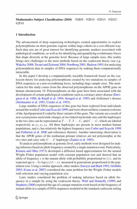
The advancement of deep sequencing technologies created opportunities to explorepolymorphisms on short genomic regions within large cohorts in a cost efficient way.Such data sets are of great interest for identifying genomic markers associated withpathological conditions, as well as for identifying and quantifying evolutionary forcesthat shape diversity at the genomic level. Because of large sample sizes, this realitybrings new challenges to the most methods based on the coalescent theory (see e.g.Wakeley 2008; Tavaré and Zeitouni 2004; Nordborg 2001; Hudson 1991) for analyzingpolymorphism data in samples of DNA sequences by making them computationallyintractable.
In this paper I develop a computationally tractable framework based on the coa-lescent theory for analyzing polymorphisms created by two mutations in samples ofDNA sequences at a non-recombining locus, including large sample sizes. The moti-vation for this study comes from the observed polymorphisms on the APOE gene onhuman chromosome 19. Polymorphisms on this gene have been associated with thedevelopment of certain pathological conditions such as coronary artery disease (Davi-gnon et al. 1988; de Knijff et al. 1994; Stengrd et al. 1995) and Alzheimer’s disease(Strittmatter et al. 1993; Corder et al. 1993).
Large number of DNA sequences of this gene has been explored from individualsaround the world (Corbo and Scacchi 1999) and were observed three common isoformsof the Apolipoprotein E coded by three variants of this gene. The variants are a result ofnon-synonymous nucleotide changes at two linked nucleotide sites and the haplotypesat the two sites can be represented as T · · · T, T · · · C, and C · · · C, which are labeledrespectively as e2, e3, e4. All three haplotypes are present in most modern humanpopulations, and e3 has relatively the highest frequency (see Corbo and Scacchi 1999and Fullerton et al. 2000 and references therein). Another interesting observation isthat the APOE genes of the nonhuman primate relatives are not polymorphic at thetwo sites and carry only C · · · C haplotype (Zannis et al. 1985).
To analyze polymorphisms at genomic level, early methods were designed for mak-ing inference based on allele frequency created by a single mutation event. Particularly,Kimura and Ohta (1973) developed a diffusion based approximation for the neutralWright–Fisher population model with constant population size and showed that anallele of frequency x is the mutant allele with probability proportional to 1/x, and itsexpected age is −2x log(x)/(1− x),measured in generations proportional to the pop-ulation size. Using a similar approach, other studies (Sawyer and Hartl 1992; Griffiths2003; Evans et al. 2007) considered the same problem for the Wright–Fisher modelswith selection and varying population size.
Later studies considered the problem of making inference based on allele fre-quency in a sample by using the coalescent theory. Wiuf and Donnelly (1999) andStephens (2000) explored the age of a unique mutation event based on the frequency ofmutant allele in a sample of DNA sequences modeled in the standard coalescent setting
123
Two mutations in the general coalescent tree setting
(Kingman 1982a,b,c; Hudson 1983; Tajima 1983), which describes genealogical his-tories of samples of DNA sequences under the neutral Wright–Fisher model with con-stant population size. Griffiths and Tavaré (1998) introduced the general coalescenttree framework and explored the inference problem in this setting. This frameworkincludes many genealogical models such as the standard coalescent, the variable-population-size coalescent model (Griffiths and Tavaré 1994; Slatkin and Hudson1991), the genealogical models derived from birth–death processes (Thompson 1975;Nee et al. 1994; Rannala 1997; Slatkin and Rannala 1997), and the genealogical mod-els for samples of DNA sequences completely linked to a mutation that is neutral orunder selection (Stephens and Donnelly 2003; Coop and Griffiths 2004; Griffiths andTavaré 2003, 1998; Slatkin and Rannala 1997).
Most of the methods mentioned above are computationally tractable including largesample sizes, but they are applicable only for polymorphisms created by a single muta-tion. To include more linked polymorphic sites into analysis, full likelihood basedinference methods (Griffiths and Tavaré 1995, 1999; Kuhner et al. 1995; Felsensteinet al. 1999; Stephens and Donnelly 2000; Hobolth et al. 2008) have been developedunder the standard coalescent and the infinite-sites model. Further extensions of thesemethods were considered for the variable-population-size coalescent model (Griffithsand Tavaré 1994, 1999; Kuhner et al. 1998) and for the general coalescent tree frame-work (Sargsyan 2010). Although these methods allow to consider many (completely)linked polymorphic sites in a sample of DNA sequences at a non-recombining locus,these methods can be computationally intractable for large sample sizes.
Instead of allowing many mutation events on the genealogy of a sample, Griffithsand Tavaré (2003) extended their work on a single mutation (Griffiths and Tavaré 1998)by considering polymorphisms crated by two mutation events that occurred on samelineage. Hobolth and Wiuf (2009) considered this problem in the standard coalescentsetting by using the recursion formula derived by Griffiths and Tavaré (1995). Forthis same setting Jenkins and Song (2011) considered a recurrent mutation scenario inwhich mutational changes created by two mutation events occur on same nucleotidesite. Xie (2011) used diffusion based approximations for the equilibrium Wright–Fisher models with and without selection to derive a method for calculating the jointdistribution of allele frequencies at two completely linked sites.
While the method by Sargsyan (2010) provides a simulation based solution for ana-lyzing polymorphisms created by two mutation events in the general coalescent treesetting, in this paper I present an analytical solution for this problem. The solution isbased on the framework that I developed in my doctoral dissertation (Sargsyan 2006).Using a different approach than the methods mentioned above, the framework is devel-oped by deriving analytical formulas for the numbers of various topological structuresof the genealogies with two mutations. These formulas allow to derive expressions forcomputing the probability of polymorphism data created by two mutation events andthe ages of the events. An advantage of this approach is that it makes the frameworkcomputationally tractable for large sample sizes. As another implication of this frame-work, I extend the definition of the site frequency spectrum by classifying all pairs ofpolymorphic sites in a sample of DNA sequences into groups and present expressionsfor computing the expected sizes of these groups. In addition, I use the framework todesign a Bayesian approach for inferring the ancestral nucleotide at the two mutant
123
O. Sargsyan
sites based on the haplotype frequencies at the two sites and apply this method to thepolymorphisms in samples of DNA sequences from the human APOE gene region.
2 Methods and results
2.1 Polymorphisms in samples of DNA sequences modeled in the general coalescenttree setting
The general coalescent tree framework models polymorphisms in a sample of DNAsequences at a non-recombining locus by describing a genealogical process combinedwith a mutation process. The genealogy of the sample represents an ancestral historyof the sample back in time before the most recent common ancestor and mutationevents on the genealogy are added according to a Poisson process with rate θ/2. Thegenealogy of n sequences is a binary tree with n leaves representing the sequences andn − 1 internal nodes representing the coalescent events; the root of the tree is the mostrecent common ancestor. Such trees are constructed according to the following processin which the waiting times between consecutive coalescent events are determined byn−1 random variables Tn, Tn−1, . . . , T2.The process is tracing the lineages recursivelybetween the coalescent events by starting with n lineages. The random variable Tn
determines the waiting time to the first coalescent event at which two randomly chosenlineages out of the n are merged into a single lineage. Similarly, the n − 1 lineagesare traced to the next coalescent event for which the waiting time is determined byTn−1. After repeating similar steps for i, i = n − 2, . . . , 2, lineages in which casethe waiting time to the next coalescent event is determined by Ti , the process stopsat the coalescent event that corresponds to the most recent common ancestor of thesample.
The sequences at the mutation events are modified according to the infinite-sitesmodel or a finite-sites model. Although within this framework many substitution mod-els can be considered for l nucleotide long sequences, I assume that mutational changesare equally likely to occur on any of the l sites. For the case of only two mutation events,substitutions can occur on same nucleotide site with probability q equal to 1/ l. For thecase of the infinite-sites model q is equal to 0 because l is considered to be ∞, thereforesubstitutions occur on nucleotide sites that have not been mutated before. Substitutionsare determined by a transition rate matrix P = {Pi, j }, i, j ∈ {A, T,G,C} and by thesequence of the most recent common ancestor of the sample.
For the case of only two mutation events on the genealogy of a sample, I denote themutation rate by θ0 to distinguish from the general case by taking into account somespecifics of this case. Particularly, θ0 can be considered to be very small (θ0 → 0)because it represents mutation rate at a locus that contains at most two substation sitesand the length of the locus can be considered to be very small under the infinite-sitesmodel. Griffiths and Tavaré (1998) used similar argument for modeling a polymor-phism at a nucleotide site created by a single mutation event. The limiting behaviorcan also be observed based on Watterson’s formula (Watterson 1975), which estimatesθ0 to be 2/
∑n−1i=1 1/ i in the standard coalescent setting and it becomes very small for
large sample sizes.
123
Two mutations in the general coalescent tree setting
2.2 The probability of polymorphism data created by two mutation events
I first explore the probability distribution of the topological structures created by twomutation events on the genealogy of n sequences; let E2 be the set of such genealo-gies. To define some of the structures, I use the relationships between mutant groupsassociated with the two mutation events. The mutant group of a mutation event on thegenealogy of DNA sequences is defined as the subset of sequences on whose lineagesthe event occurred. Because two mutation events can be on same lineage or on distinctlineages of the genealogy, their mutant groups can be nested or disjoint. Let E2r andE2h be the sets of the genealogies representing each of these cases, respectively. Thereare more structures within these sets: In the case of E2r , mutant groups are strictlynested or identical; let E2r,n and E2r,s be these possibilities, respectively. In the case ofE2h, the mutant groups are strictly disjoint or complementary (their union is the wholesample); let E2h,d and E2h,c be these cases, respectively. In the following theorem Iderive expressions for computing the probabilities of these events conditional on E2.
Theorem 1 Let rn and hn be the probabilities of E2r and E2h conditional on E2. Thefollowing properties and representations hold for rn and hn :(a) rn + hn = 1.(b) The probabilities of rn and hn are independent from the topology of the genealogy.(c) The following formula holds for rn :
rn = IE((nS2
2 − ∑ni=2(S2 − Si )
2)e−θ0 Ln/2)
IE(L2
ne−θ0 Ln/2) . (1)
(d) The inequality
hn > rn,
holds when n > 2. This means that two mutation events are more likely to occuron distinct lineages than on same lineage.
(e) The probabilities of the events E2r,n, E2r,s, E2h,d , and E2h,c conditional on E2can be evaluated based on the following expressions:
IP(E2r,s | E2) =∑
2≤k≤m≤nk(k−1)m−1 dm,kIE
(Tm Tke−θ0 Ln/2
)
IE((L2
n/2)e−θ0 Ln/2) , (2)
IP(E2r,n | E2) = rn − IP(E2r,s | E2), (3)
IP(E2r,c | E2) =∑
2≤m≤n2
m−1 dm,2IE(Tm T2e−θ0 Ln/2
)
IE((L2
n/2)e−θ0 Ln/2
) , (4)
IP(E2h,d | E2) = hn − IP(E2h,c | E2). (5)
Here dm,k = 1/2 if m = k, otherwise dm,k = 1.
The proof of the theorem is in the Appendix.
123
O. Sargsyan
To estimate the probability of polymorphism data Dn in a sample of n DNAsequences under the general coalescent tree setting and a given sequence α for the mostrecent common ancestor of the sample, one can consider the Monte Carlo approach.That is, by generating very large number of independent samples of n sequences andtaking the proportion of generated data sets that match with Dn . Samples are gener-ated by constructing random genealogical histories according to the general coalescenttree framework and adding mutation events on the genealogies, and then implementingsubstations at mutation events based on the sequence α.Although this approach mightbe computationally intractable, it gives a description for the probabilities of polymor-phism data under the general coalescent tree setting. For the case of polymorphismscreated by two mutation events, below I apply this approach to derive expressions forcomputing the probability of Dn conditional on (α, E2). This probability can be rep-resented as a sum by considering all possible transition histories Hα at two mutationevents under specified α:
IP(Dn | α, E2) =∑
Hα
IP(Dn | Hα, α, E2)IP(Hα | α, E2). (6)
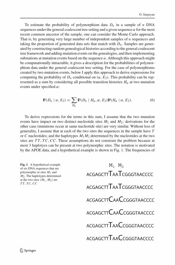
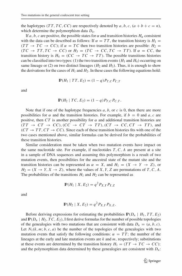
To derive expressions for the terms in this sum, I assume that the two mutationevents have impact on two distinct nucleotide sites M1 and M2; derivations for theother case (mutations occur at same nucleotide site) are very similar. Without loss ofgenerality, I assume that at each of the two sites the sequences in the sample have Tor C nucleotides; and the haplotypes M1 M2 determined by the nucleotides at the twosites are T T, T C,CC. These assumptions do not constrain the problem because atmost 3 haplotyes can be present at two polymorphic sites. The notation is motivatedby the APOE data, and a hypothetical example is shown in Fig. 1. The frequencies of
Fig. 1 A hypothetical exampleof six DNA sequences that arepolymorphic at sites M1 andM2. The haplotypes determinedat the two sites (M1,M2) areT T, T C,CC
123
Two mutations in the general coalescent tree setting
the haplotypes (T T, T C,CC) are respectively denoted by a, b, c, (a + b + c = n),which determine the polymorphism data Dn .
If a, b, c are positive, the possible states for α and transition histories Hα consistentwith the data can be described as follows: If α = T T , the transition history is H1 =(T T → T C → CC); if α = T C then two transition histories are possible: H2 =(T C → T T, T C → CC) or H3 = (T C → CC, T C → T T ). If α = CC, thetransition history is H4 = (CC → T C → T T ). The possible transitions historiescan be classified into two types: (1) the two transition events (H1 and H4) occurring onsame lineage or (2) on two distinct lineages (H2 and H3). Thus, it is enough to showthe derivations for the cases of H1 and H2. In these cases the following equations hold:
IP(H1 | T T, E2) = (1 − q)PT,C PC,T
and
IP(H2 | T C, E2) = (1 − q)PT,C PC,T .
Note that if one of the haplotype frequencies a, b, or c is 0, then there are morepossibilities for α and the transition histories. For example, if b = 0 and a, c arepositive, then CT is another possibility for α and additional transition histories are(T T → CT → CC), (CC → CT → T T ), (CT → CC,CT → T T ), and(CT → T T,CT → CC). Since each of these transition histories fits with one of thetwo cases mentioned above, similar formulas can be derived for the probabilities ofthese transition histories.
Similar consideration must be taken when two mutation events have impact onthe same nucleotide site. For example, if nucleotides T,C, A are present at a sitein a sample of DNA sequences and assuming this polymorphism is a result of twomutation events, then possibilities for the ancestral state of the mutant site and thetransition histories can be represented as α = X, and H1 = (X → Y → Z), orH2 = (X → Y, X → Z), where the values of X,Y, Z are permutations of T,C, A.The probabilities of the transitions H1 and H2 can be represented as
IP(H1 | X, E2) = q2 PX,Y PY,Z
and
IP(H2 | X, E2) = q2 PX,Y PX,Z .
Before deriving expressions for estimating the probabilities IP(Dn | H1, T T, E2)
and IP(Dn | H2, T C, E2), I first derive formulas for the number of possible topologiesof the genealogies with two mutations that are consistent with data Dn = (a, b, c).Let N1(k,m; b, c, a) be the number of the topologies of the genealogies with twomutation events that satisfy the following conditions: α = T T ; the number of thelineages at the early and late mutation events are k and m, respectively; substitutionsat these events are determined by the transition history H1 = (T T → T C → CC);and the polymorphism data determined by these genealogies are consistent with Dn :
123
O. Sargsyan
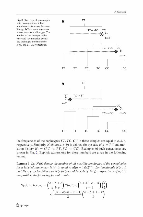
Fig. 2 Two type of genealogieswith two mutations. a Twomutation events are on the samelineage. b Two mutation eventsare on two distinct lineages. Thenumber of the lineages at theearly and late mutation eventsand their ages are denoted byk,m, and ξ1, ξ2, respectively
a
b
the frequencies of the haplotypes T T, T C,CC in these samples are equal to a, b, c,respectively. Similarly, N2(k,m; a, c, b) is defined for the case of α = T C and tran-sition history H2 = (T C → T T, T C → CC). Examples of such genealogies areshown in Fig. 2. Explicit expressions for these numbers are given in the followinglemma.
Lemma 1 Let N (n) denote the number of all possible topologies of the genealogiesfor n labeled sequences; N (n) is equal to n!(n − 1)!/2n−1. Let functionals N (x, y)and N (x, y, z) be defined as N (x)N (y) and N (x)N (y)N (z), respectively. If a, b, care positive, the following formulas hold:
N1(k,m; b, c, a) =(
a + b + c
a b c
)
N (a, b, c)
(a + b + c − m
c − 1
)(k
2
)
×[(m − a)(m − a − 1)
2
(a + b + 1 − k
b
)
123
Two mutations in the general coalescent tree setting
+ (m − a)(a + b + 1 − m)
(a + b − k
b
)
+ (a + b + 1 − m)(a + b − m)
2
(a+b − k − 1
b
)]
, (7)
in which (k,m) satisfies the condition
(k,m) ∈ Δ1(b, c, a) ≡ {(k,m) : 2 ≤ k ≤ min(a + 1,m − 1), 3 ≤ m ≤ b + a + 1},
and
N2(k,m; a, c, b) ≡(
a + b + c
a b c
)
N (a, b, c)
(a + b + c − m
c − 1
)(k
2
)
×[(m − a)(m − a − 1)
2
(a + b − k + 1
a − 1
)
+ (m − a)(a + b − m + 1)
(a + b − k
a − 2
)
+ (a + b−m + 1)(a + b − m)
2
(a + b − k − 1
a − 3
)]
, (8)
in which (k,m) satisfies the condition
(k,m) ∈ Δ2(a, c, b) ≡ {(k,m) : 2 ≤ k ≤ min(b + 2,m), 3 ≤ m ≤ a + b + 1}.
If b = 0 and α = T T, the two mutant groups are the same and
N1(k,m; 0, c, a) =(
a + c
a
)
N (a, c)
(a + c − m
c − 1
)(k
2
)
,
in which (k,m) satisfies the condition
(k,m) ∈ Δ1(0, c, a) ≡ {(k,m) : 2 ≤ k ≤ m ≤ a + 1};
if α = T C, the two mutant groups are complementary and
N2(k,m; a, c, 0) ≡(
a + c
a
)
N (a, c)
(a + c − m
c − 1
)
,
(k,m) ∈ Δ2(a, c, 0) ≡ {(k,m) : k = 2, 2 ≤ m ≤ a + 1}. Note that the binomial
coefficient
(x
z
)
is equal to 0 if x < z or z < 0.
The proof of the lemma is in the Appendix.
123
O. Sargsyan
Note that the numbers of the topologies of the genealogies with two mutations forthe cases of {α = CC, H4} and {α = T C, H3}, can be computed as N1(k,m; b, a, c),(k,m) ∈ Δ1(b, a, c), and N2(k,m; c, a, b), (k,m) ∈ Δ2(c, a, b), respectively.
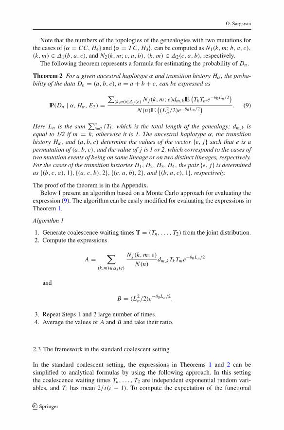
The following theorem represents a formula for estimating the probability of Dn .
Theorem 2 For a given ancestral haplotype α and transition history Hα, the proba-bility of the data Dn = (a, b, c), n = a + b + c, can be expressed as
IP(Dn | α, Hα, E2) =∑(k,m)∈Δ j (e) N j (k,m; e)dm,kIE
(Tk Tme−θ0 Ln/2
)
N (n)IE((L2
n/2)e−θ0 Ln/2) . (9)
Here Ln is the sum∑n
i=2 iTi , which is the total length of the genealogy; dm,k isequal to 1/2 if m = k, otherwise it is 1. The ancestral haplotype α, the transitionhistory Hα, and (a, b, c) determine the values of the vector {e, j} such that e is apermutation of (a, b, c), and the value of j is 1 or 2, which correspond to the cases oftwo mutation events of being on same lineage or on two distinct lineages, respectively.For the cases of the transition histories H1, H2, H3, H4, the pair {e, j} is determinedas {(b, c, a), 1}, {(a, c, b), 2}, {(c, a, b), 2}, and {(b, a, c), 1}, respectively.
The proof of the theorem is in the Appendix.Below I present an algorithm based on a Monte Carlo approach for evaluating the
expression (9). The algorithm can be easily modified for evaluating the expressions inTheorem 1.
Algorithm 1
1. Generate coalescence waiting times T = (Tn, . . . , T2) from the joint distribution.2. Compute the expressions
A =∑
(k,m)∈Δ j (e)
N j (k,m; e)
N (n)dm,k Tk Tme−θ0 Ln/2
and
B = (L2n/2)e
−θ0 Ln/2.
3. Repeat Steps 1 and 2 large number of times.4. Average the values of A and B and take their ratio.
2.3 The framework in the standard coalescent setting
In the standard coalescent setting, the expressions in Theorems 1 and 2 can besimplified to analytical formulas by using the following approach. In this settingthe coalescence waiting times Tn, . . . , T2 are independent exponential random vari-ables, and Ti has mean 2/ i(i − 1). To compute the expectation of the functional
123
Two mutations in the general coalescent tree setting
φ(Tn, . . . , T2)e− θ02 Ln , I use Griffiths and Tavaré’s (2003) approach by representing
the expectation as the expectation from the functional Cθ0,nφ(T̃n, . . . , T̃2), in whichT̃n, . . . , T̃2 are independent exponential random variables, T̃i has rate i(i −1+ θ0)/2,and Cθ0,n is equal to
∏ni=2
i−1i−1+θ0
. For example, after applying this approach to theexpectations in (9), the following equations hold:
IE(L2ne−θ0 Ln/2) = Cθ0,n
⎛
⎝n∑
j=2
4
( j − 1 + θ0)2+
(n∑
i=2
2
i − 1 + θ0
)2⎞
⎠ ,
IE(Tk Tme−θ0 Ln/2) = Cθ0,nIE(T̃k T̃m),
where IE(T̃k T̃m) is equal to
4
k(k − 1 + θ0)m(m − 1 + θ0)
if k �= m, otherwise it is equal to
8
(k(k − 1 + θ0))2.
2.4 Extension of the site frequency spectrum
Under the infinite-sites model the site frequency spectrum for polymorphisms in asample of n DNA sequences is described as vector ( f1, f2, . . . , fn−1), where fi isthe count of polymorphic sites at which the frequencies of the mutant and ancestralalleles are respectively equal to i and n − i. As an alternative, this statistics can bedefined by classifying polymorphic sites into groups according to the equivalencerelationship described as follows. Under the infinite-sites model, two polymorphicsites in a sample of DNA sequences are considered to be equivalent if the frequenciesof the mutant alleles at the two sites are the same. In the standard coalescent setting,Fu (1995) showed that the expected value of fi is equal to θ/ i. Griffiths and Tavaré(1998) extended this result in the general coalescent tree setting.
Before extending the definition of the site frequency spectrum, I explore some of thefeatures of pairs of polymorphic sites in a sample of DNA sequences. Under the infinite-sites model, any two polymorphic sites at a non-recombining locus can be characterizedby the relationships between the mutant groups associated with the polymorphisms.The set of all pairs of polymorphic sites in a sample can be partitioned into two groupsaccording to the relationship between mutant groups of each pair of polymorphic sites:the mutant groups are disjoint or nested. Let Hn and Rn be respectively the expectedsizes of these groups for a sample of size n in the general coalescent tree setting, andthese quantities can be computed based on the following formulas:
Rn = 1
2
(θ
2
)2
IE
(
nS22 −
n∑
i=2
(S2 − Si )2
)
, (10)
123
O. Sargsyan
Hn = 1
2
(θ
2
)2
IE
(
L2n − nS2
2 +n∑
i=2
(S2 − Si )2
)
. (11)
To derive these expressions as well as the others below, I used formulas (1–5), (9), andarguments similar to those used by Nielsen (2000) and Griffiths and Tavaré (1998) forsite frequency spectrum (details not shown).
To explore further structures in the set of all pairs of polymorphic sites in a sample,I partition this set into four groups depending on the mutant groups of the pair ofpolymorphic sites that are strictly nested, equal, strictly disjoint, or complementary.Let Rn,n, Rn,s, Hn,d , Hn,c be the expected sizes of these groups, respectively. Thesequantities can be computed based on the following formulas:
Rn,s =(θ
2
)2 ∑
2≤k≤m≤n
k(k − 1)
m − 1dm,kIE (Tm Tk), (12)
Rn,n = Rn − Rn,s, (13)
Hn,c =(θ
2
)2 ∑
2≤m≤n
2
m − 1dm,2IE (Tm T2), (14)
Hn,d = Hn − Hn,c. (15)
Recall that dm,k = 1/2 if m = k, otherwise dm,k = 1.More detailed characterization for pairs of polymorphic sites is based on deter-
mining the values of the statistics α, j, Dn, Hα as described in the previous sectionand defining pairs of polymorphic sites to be equivalent if they have the same valuesfor the statistics j and Dn . Based on this equivalence relation the definition of thesite frequency spectrum is extended by classifying all pairs of polymorphic sites intogroups. Let SDn , j be the expected number of pairs of polymorphic sites in a sampleof n DNA sequences that represent the polymorphism data { j, Dn}. This quantity canbe computed based on the following formulas:
SDn , j =∑
Hα
SDn , j,Hα , (16)
in which
SDn , j,Hα =(θ
2
)2 ∑
(k,m)∈Δ j (e)
N j (k,m; e)
N (n)dm,kIE (Tk Tm).
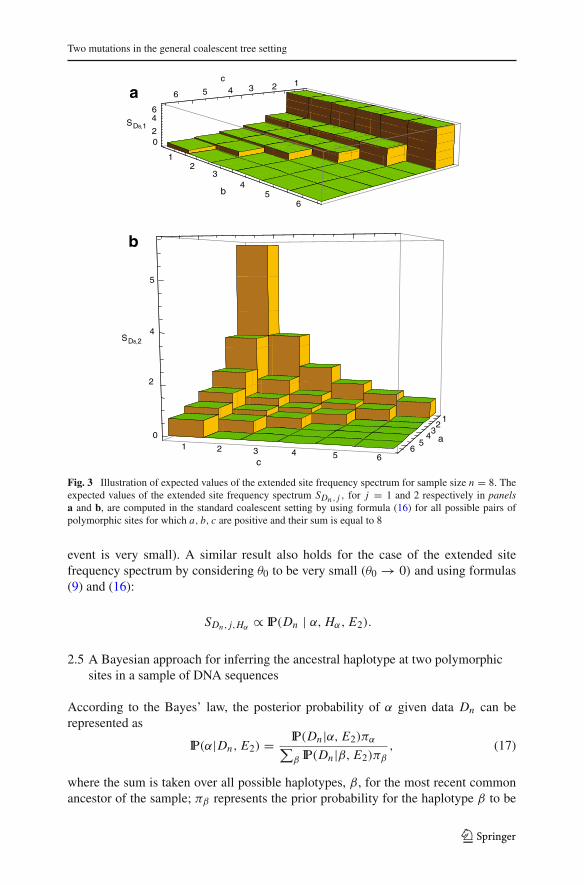
For sample size n = 8, the expected values SDn , j are illustrated in Fig. 3 for a constantpopulation size model.
Note that Griffiths and Tavaré (1998) showed that the expected site frequencyspectrum in a sample of n DNA sequences modeled in the general coalescent treesetting is proportional to the probability distribution of the frequency of a mutantallele created by a single mutation event (assuming mutation rate for a single mutation
123
Two mutations in the general coalescent tree setting
15 3
6 4 2
12
34
5
4
1 2 3 4 5 6
12
34
56
6
a
b
6
20
5
4
2
0
c
a
b
c
D8,1S
D8,2S
Fig. 3 Illustration of expected values of the extended site frequency spectrum for sample size n = 8. Theexpected values of the extended site frequency spectrum SDn , j , for j = 1 and 2 respectively in panelsa and b, are computed in the standard coalescent setting by using formula (16) for all possible pairs ofpolymorphic sites for which a, b, c are positive and their sum is equal to 8
event is very small). A similar result also holds for the case of the extended sitefrequency spectrum by considering θ0 to be very small (θ0 → 0) and using formulas(9) and (16):
SDn , j,Hα ∝ IP(Dn | α, Hα, E2).
2.5 A Bayesian approach for inferring the ancestral haplotype at two polymorphicsites in a sample of DNA sequences
According to the Bayes’ law, the posterior probability of α given data Dn can berepresented as
IP(α|Dn, E2) = IP(Dn|α, E2)πα∑β IP(Dn|β, E2)πβ
, (17)
where the sum is taken over all possible haplotypes, β, for the most recent commonancestor of the sample; πβ represents the prior probability for the haplotype β to be
123
O. Sargsyan
the ancestral haplotype. The probabilities on the right side of the above equation canbe evaluated by using the results in Sect. 2.2.
To make the developed framework applicable for large sample sizes, in the followinglemma I first explore the asymptotic behaviors of N1() and N2() when a, b, c arepositive. Note that similar methods can be applied to derive asymptotic formulas forthe case of b = 0.
Lemma 2 Under the limits an → x, b
n → y, cn → z, as a, b, c tend to ∞, the
following asymptotic formulas hold:
N1(k,m; b, c, a)N (n)n2
→ D1(y, k; z,m), 3 ≤ m, 2 ≤ k ≤ m − 1, (18)
N1(k,m; b, a, c)N (n)n2
→ D1(y, k; x,m), 3 ≤ m, 2 ≤ k ≤ m − 1, (19)
N2(k,m; a, c, b)N (n)n2
→ D2(x, k; z,m), 3 ≤ m, 2 ≤ k ≤ m, (20)
N2(k,m; c, a, b)N (n)n2
→ D2(z, k; x,m), 3 ≤ m, 2 ≤ k ≤ m; (21)
where
D1(y, k; z,m) ≡ k(k − 1)(m − k)(2xk−1 + xk−2 y(m − k + 1))
(x + y)k−m+2
and
D2(x, k; z,m) ≡ k(k − 1)yk−3
(x + y)k−m+2
(x2(k − 1)(k − 2)+ 2xy(k − 1)(m − 2)
+ y2(m − 1)(m − 2)).
The proof of the lemma is in the Appendix.Based on the above asymptotic limits, I derive analytical expressions for the pos-
terior distribution (17) in the standard coalescent setting.
Theorem 3 Under the limits θ0 → 0, a/n → x, b/n → y, and c/n → z asa, b, c → ∞, the expressions (17) for the posterior probabilities of the haplotypesT T, T C,CC can be represented as
IP(T T |(x, y, z), E2) = F(z)πT T
P D, (22)
IP(T C |(x, y, z), E2) =(
4xz − F(x)− F(z)
)πT C
P D, (23)
IP(CC |(x, y, z), E2) = F(x)πCC
P D, (24)
123
Two mutations in the general coalescent tree setting
in which
F(x) ≡ 4(1 − x2 + 2x log(x))
x(1 − x)3,
and
P D =(
4
xz− F(x)− F(z)
)
πT C + F(z)πT T + F(x)πCC .
The proof of the theorem is in the Appendix.
2.6 Conditional distributions of the ages of two mutation events
In this section I derive expressions for estimating the distributions of the ages of earlyand late mutation events and the time of the most recent common ancestor conditionalon Dn . Let ξ1, ξ2, and ξ denote the ages of the early and late mutation events, and thetime of the most recent common ancestor, respectively.
Theorem 4 The joint distribution of (ξ1, ξ2, ξ) conditional on {Dn, α, Hα, E2} canbe estimated based on the expression
IP(ξ1 ≤ t1, ξ2 ≤ t2, ξ ≤ t | Dn, α, Hα, E2)
=∑(k,m)∈Δ j (e) N j (k,m; e)IE
(K (k, t1; m, t2)I{S2 ≤ t}e−θ0 Ln/2
)
∑(k,m)∈Δ j (e) N j (k,m; e)dm,kIE
(Tm Tke−θ0 Ln/2
) , (25)
where Si is the sum∑n
j=i Tj , Ln = ∑ni=2 iTi , and I{x} is 1 if x is true, otherwise it
is 0. The functional K (k, t1; m, t2) is defined as follows:
K (k, t1; m, t2) =⎧⎨
⎩
K (k, t1)K (m, t2) if k �= m,K (k, t1)2/2 if k = m and t1 < t2,K (k, t1)K (k, t2)− K (k, t2)2/2 if k = m and t2 < t1.
The functional K (i, p) is defined as Ti ∧ (p − Si+1)+, in which x ∧ y = min(x, y)and (a)+ is equal to a if a > 0, otherwise it is 0.
The proof of the theorem is in the Appendix.I use this theorem to derive conditional distribution of ξ1, and its first and second
moments. Similar derivations can be applied for the cases of ξ2 and ξ . The probabilitydistribution of ξ1 follows from the above joint distribution by taking t2 and t to infinity:
IP(ξ1 ≤ t1 | Dn, α, Hα, E2)=∑(k,m)∈Δ j (e) N j (k,m; e)IE
(K (k, t1; m,∞)e−θ0 Ln/2
)
∑(k,m)∈Δ j (e) N j (k,m; e)dm,kIE
(Tk Tme−θ0 Ln/2
) .
123
O. Sargsyan
In this expression K (k, t1; m,∞) simplifies as follows: if k �= m then K (k, t1; m,∞)
is equal to K (k, t1)Tm, otherwise K (k, t1; k,∞) is equal to K (k, t1)2/2. To com-pute the first and second moments of ξ1 conditional on {Dn, Hα, E2}, the for-mula for the probability distribution of ξ1 is applied to the well known formulaIEXi = ∫ ∞
0 xi−1IP(X > x)dx . Thus, the moments are expressed as
IE(ξ i1 | Dn, α, Hα, E2) =
∑(k,m)∈Δ j (e) N j (k,m; e)IE
(ψk,m(T, i)e−θ0 Ln/2
)
∑(k,m)∈Δ j (e) N j (k,m; e)dm,kIE
(Tk Tme−θ0 Ln/2
) , (26)
in which
ψk,m(T, i) =∞∫
0
t i−1(dm,k Tk Tm − K (k, t; m,∞))dt, i = 1, 2,
and it simplifies to
ψk,m(T, 1) ={
Tk Tm(Sk + Sk+1)/2 if k �= m,T 2
k (2Sk + Sk+1)/6 if k = m
and
ψk,m(T, 2) ={
Tk Tm(S2k + Sk Sk+1 + S2
k+1)/3 if k �= m,
T 2k (6S2
k + 4Sk Sk+1 + 2S2k+1)/24 if k = m.
For the first and second moments of ξ2 the right side of Eq. (26) can be used afterredefining ψk,m(T, i), i = 1, 2, as
ψk,m(T, 1) ={
Tk Tm(Sm + Sm+1)/2 if k �= m,T 2
m(Sm + 2Sm+1)/6 if k = m
and
ψk,m(T, 2) ={
Tk Tm(S2m + Sm Sm+1 + S2
m+1)/3 if k �= m,
T 2m(2S2
m + 4Sm Sm+1 + 6S2m+1)/24 if k = m.
Similar formulas can also be derived for the first and second moments of ξ.
2.7 Asymptotic behavior of the expected ages of two mutation events in the standardcoalescent setting for large sample sizes
In the following theorem, I present asymptotic limits of the expected ages of early andlate mutation events for large sample sizes modeled in the standard coalescent setting.
123
Two mutations in the general coalescent tree setting
Theorem 5 Under the conditions θ0 → 0, a/n → x, b/n → y, and c/n → z, asa, b, c → ∞, the expected ages of two mutation events in the standard coalescentsetting can be computed based on the following analytical formulas. If α = T Tand Hα = H1, the expected ages (ξ1 and ξ2) of the early and late mutation eventsconditional on (x, y, z) can be computed based on the formulas
IE(ξ1|(x, y, z), T T , H1) = D1,1(z, y, x)
F(z), (27)
IE(ξ2|(x, y, z), T T , H1) = D1,0(z, y, x)
F(z)(28)
Ifα = T C and the transition histories are {H2, H3}, let ξT C,T T and ξT C,CC be respec-tively the ages of the transition events T C → T T and T C → CC. For large samplesizes the expected ages of these statistics conditional on {x, y, z} can be computedbased on the formulas
IE(ξT C,T T | (x, y, z), T C, H2, H3) = D2,1(x, z, y)+ D2,0(z, x, y)− D2,2(y)4zx − F(x)− F(z)
,
(29)
IE(ξT C,CC | (x, y, z), T C, H2, H3) = D2,1(z, x, y)+ D2,0(x, z, y)− D2,2(y)4zx − F(x)− F(z)
.
(30)
The proof of the theorem is in the Appendix. Note that formula (28) was alsoderived by Griffiths and Tavaré (2003) (formula (8.8) in their article), in their formulathe number 4 is a typo and it must be 2.
The notations in the theorem are defined as follows:
D1,0(x, y, z) ≡ −8((1 + x) log(x)− 2x + 2)
(1 − x)3,
D1,1(x, y, z) ≡ 16 log(1 − z) log(x)
(1 − x)3
+ 16
(1 − x)3
1∫
0
log(1 − (y + z)t)
(z
1 − zt− 1
t
)
dt
+8(x2 − y2) log(1 − z)
yzx(1 − x)+ 8 log(x)(2y − x(1 − x))
y(1 − x)3,
G(t) ≡ 1 − t2 + 2t log(t)
t (1 − t),
D2,0(x, y, z) ≡ −8(y2 + (1 − z)(1 − x)2) log(1 − z)
yz3(1 − x)− 16
z2
+(
x
y− 2
1 − x
)8 log(x)
(1 − x)2− 16PolyLog(2, 1 − x)
(1 − x)3
123
O. Sargsyan
+ 8z
(1 − x)2
1∫
0
G(x)− G(1 − zt)
1 − zt − xdt,
D2,1(x, y, z) ≡ 8
1 − x− 8z log(x)
y(1 − x)2+ 8(1 − x2 + 2x log(x))
(1 − x)3+ 8 log(1 − z)
yz
−40
z2 + 8(−3 + 2z) log(1 − z)
z3 + 16PolyLog(2, z)
z3 ,
D2,2(z) ≡ −56
z2 − 8(5 − 3z) log(1 − z)
z3 + 16PolyLog(2, z)
z3 ,
where PolyLog(i, z) is for the Polylogarithm function defined as∑∞
k=1 zk/ki .
2.8 Application
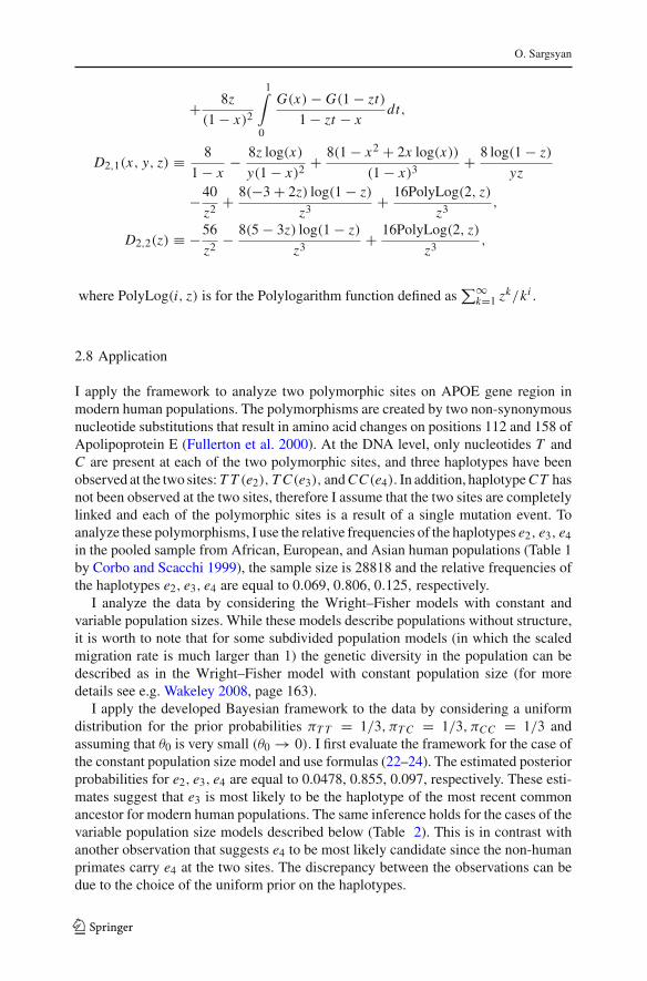
I apply the framework to analyze two polymorphic sites on APOE gene region inmodern human populations. The polymorphisms are created by two non-synonymousnucleotide substitutions that result in amino acid changes on positions 112 and 158 ofApolipoprotein E (Fullerton et al. 2000). At the DNA level, only nucleotides T andC are present at each of the two polymorphic sites, and three haplotypes have beenobserved at the two sites: T T (e2), T C(e3), and CC(e4). In addition, haplotype CT hasnot been observed at the two sites, therefore I assume that the two sites are completelylinked and each of the polymorphic sites is a result of a single mutation event. Toanalyze these polymorphisms, I use the relative frequencies of the haplotypes e2, e3, e4in the pooled sample from African, European, and Asian human populations (Table 1by Corbo and Scacchi 1999), the sample size is 28818 and the relative frequencies ofthe haplotypes e2, e3, e4 are equal to 0.069, 0.806, 0.125, respectively.
I analyze the data by considering the Wright–Fisher models with constant andvariable population sizes. While these models describe populations without structure,it is worth to note that for some subdivided population models (in which the scaledmigration rate is much larger than 1) the genetic diversity in the population can bedescribed as in the Wright–Fisher model with constant population size (for moredetails see e.g. Wakeley 2008, page 163).
I apply the developed Bayesian framework to the data by considering a uniformdistribution for the prior probabilities πT T = 1/3, πT C = 1/3, πCC = 1/3 andassuming that θ0 is very small (θ0 → 0). I first evaluate the framework for the case ofthe constant population size model and use formulas (22–24). The estimated posteriorprobabilities for e2, e3, e4 are equal to 0.0478, 0.855, 0.097, respectively. These esti-mates suggest that e3 is most likely to be the haplotype of the most recent commonancestor for modern human populations. The same inference holds for the cases of thevariable population size models described below (Table 2). This is in contrast withanother observation that suggests e4 to be most likely candidate since the non-humanprimates carry e4 at the two sites. The discrepancy between the observations can bedue to the choice of the uniform prior on the haplotypes.
123
Two mutations in the general coalescent tree setting
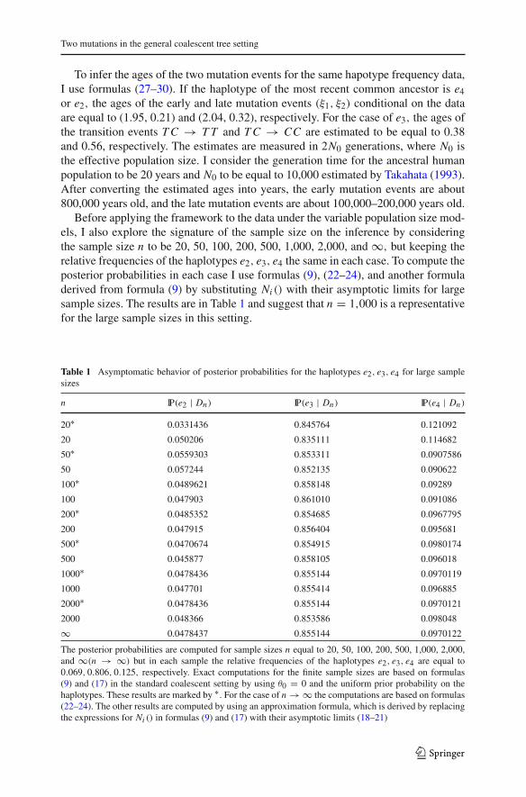
To infer the ages of the two mutation events for the same hapotype frequency data,I use formulas (27–30). If the haplotype of the most recent common ancestor is e4or e2, the ages of the early and late mutation events (ξ1, ξ2) conditional on the dataare equal to (1.95, 0.21) and (2.04, 0.32), respectively. For the case of e3, the ages ofthe transition events T C → T T and T C → CC are estimated to be equal to 0.38and 0.56, respectively. The estimates are measured in 2N0 generations, where N0 isthe effective population size. I consider the generation time for the ancestral humanpopulation to be 20 years and N0 to be equal to 10,000 estimated by Takahata (1993).After converting the estimated ages into years, the early mutation events are about800,000 years old, and the late mutation events are about 100,000–200,000 years old.
Before applying the framework to the data under the variable population size mod-els, I also explore the signature of the sample size on the inference by consideringthe sample size n to be 20, 50, 100, 200, 500, 1,000, 2,000, and ∞, but keeping therelative frequencies of the haplotypes e2, e3, e4 the same in each case. To compute theposterior probabilities in each case I use formulas (9), (22–24), and another formuladerived from formula (9) by substituting Ni () with their asymptotic limits for largesample sizes. The results are in Table 1 and suggest that n = 1,000 is a representativefor the large sample sizes in this setting.
Table 1 Asymptomatic behavior of posterior probabilities for the haplotypes e2, e3, e4 for large samplesizes
n IP(e2 | Dn) IP(e3 | Dn) IP(e4 | Dn)
20∗ 0.0331436 0.845764 0.121092
20 0.050206 0.835111 0.114682
50∗ 0.0559303 0.853311 0.0907586
50 0.057244 0.852135 0.090622
100∗ 0.0489621 0.858148 0.09289
100 0.047903 0.861010 0.091086
200∗ 0.0485352 0.854685 0.0967795
200 0.047915 0.856404 0.095681
500∗ 0.0470674 0.854915 0.0980174
500 0.045877 0.858105 0.096018
1000∗ 0.0478436 0.855144 0.0970119
1000 0.047701 0.855414 0.096885
2000∗ 0.0478436 0.855144 0.0970121
2000 0.048366 0.853586 0.098048
∞ 0.0478437 0.855144 0.0970122
The posterior probabilities are computed for sample sizes n equal to 20, 50, 100, 200, 500, 1,000, 2,000,and ∞(n → ∞) but in each sample the relative frequencies of the haplotypes e2, e3, e4 are equal to0.069, 0.806, 0.125, respectively. Exact computations for the finite sample sizes are based on formulas(9) and (17) in the standard coalescent setting by using θ0 = 0 and the uniform prior probability on thehaplotypes. These results are marked by ∗. For the case of n → ∞ the computations are based on formulas(22–24). The other results are computed by using an approximation formula, which is derived by replacingthe expressions for Ni () in formulas (9) and (17) with their asymptotic limits (18–21)
123
O. Sargsyan
N2
Te
N0
N1
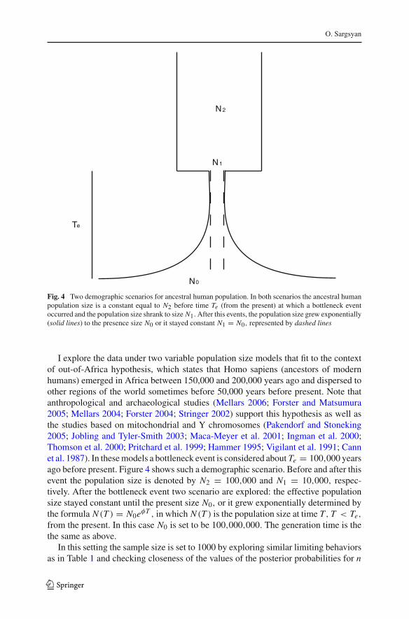
Fig. 4 Two demographic scenarios for ancestral human population. In both scenarios the ancestral humanpopulation size is a constant equal to N2 before time Te (from the present) at which a bottleneck eventoccurred and the population size shrank to size N1.After this events, the population size grew exponentially(solid lines) to the presence size N0 or it stayed constant N1 = N0, represented by dashed lines
I explore the data under two variable population size models that fit to the contextof out-of-Africa hypothesis, which states that Homo sapiens (ancestors of modernhumans) emerged in Africa between 150,000 and 200,000 years ago and dispersed toother regions of the world sometimes before 50,000 years before present. Note thatanthropological and archaeological studies (Mellars 2006; Forster and Matsumura2005; Mellars 2004; Forster 2004; Stringer 2002) support this hypothesis as well asthe studies based on mitochondrial and Y chromosomes (Pakendorf and Stoneking2005; Jobling and Tyler-Smith 2003; Maca-Meyer et al. 2001; Ingman et al. 2000;Thomson et al. 2000; Pritchard et al. 1999; Hammer 1995; Vigilant et al. 1991; Cannet al. 1987). In these models a bottleneck event is considered about Te = 100,000 yearsago before present. Figure 4 shows such a demographic scenario. Before and after thisevent the population size is denoted by N2 = 100,000 and N1 = 10,000, respec-tively. After the bottleneck event two scenario are explored: the effective populationsize stayed constant until the present size N0, or it grew exponentially determined bythe formula N (T ) = N0eφT , in which N (T ) is the population size at time T, T < Te,
from the present. In this case N0 is set to be 100,000,000. The generation time is thethe same as above.
In this setting the sample size is set to 1000 by exploring similar limiting behaviorsas in Table 1 and checking closeness of the values of the posterior probabilities for n
123
Two mutations in the general coalescent tree setting
equal to 1,000 and 2,000 (details not shown). For the computations, I use Algorithm 1and the following procedure for generating the waiting times Ti between consecutivecoalescence events in the variable population size coalescent models. Let Svi be thewaiting time (from the present) to the coalescent event at which the number of thelineages declines from i to i − 1. These quantities determine Ti as follows:
Tn = Svn ,
Ti = Svi − Svi+1, i < n.
In the mean time, Svi can be simulated by generating Sck which is a sum (Sc
k = ∑kj=n η j )
of independent exponential random variables η j with mean 2/( j ( j − 1)), j =2, . . . , n, and then using the formula of Griffiths and Tavaré (1998):
Svk = Λ−1(Sck ), k = 2, . . . , n, (31)
in which the function Λ−1() for the above described models are determined by theformula
Λ−1(y) =⎧⎨
⎩
te + γ(
y − te1−e−φφ
)if y ≥ te(1 − e−φ)/φ,
−telog(1−yφ/te)
φif y < te(1 − e−φ)/φ,
(32)
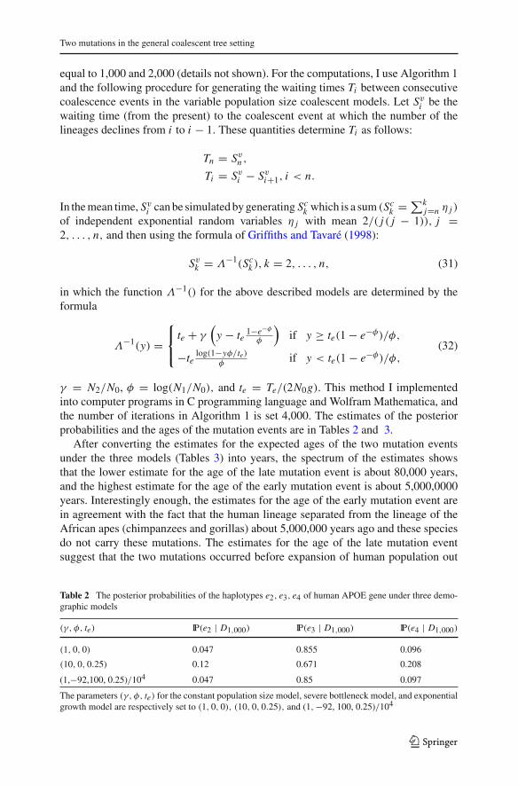
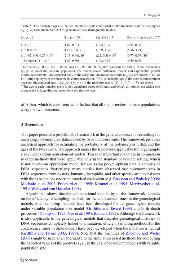
γ = N2/N0, φ = log(N1/N0), and te = Te/(2N0g). This method I implementedinto computer programs in C programming language and Wolfram Mathematica, andthe number of iterations in Algorithm 1 is set 4,000. The estimates of the posteriorprobabilities and the ages of the mutation events are in Tables 2 and 3.
After converting the estimates for the expected ages of the two mutation eventsunder the three models (Tables 3) into years, the spectrum of the estimates showsthat the lower estimate for the age of the late mutation event is about 80,000 years,and the highest estimate for the age of the early mutation event is about 5,000,0000years. Interestingly enough, the estimates for the age of the early mutation event arein agreement with the fact that the human lineage separated from the lineage of theAfrican apes (chimpanzees and gorillas) about 5,000,000 years ago and these speciesdo not carry these mutations. The estimates for the age of the late mutation eventsuggest that the two mutations occurred before expansion of human population out
Table 2 The posterior probabilities of the haplotypes e2, e3, e4 of human APOE gene under three demo-graphic models
(γ, φ, te) IP(e2 | D1,000) IP(e3 | D1,000) IP(e4 | D1,000)
(1, 0, 0) 0.047 0.855 0.096
(10, 0, 0.25) 0.12 0.671 0.208
(1,−92,100, 0.25)/104 0.047 0.85 0.097
The parameters (γ, φ, te) for the constant population size model, severe bottleneck model, and exponentialgrowth model are respectively set to (1, 0, 0), (10, 0, 0.25), and (1,−92, 100, 0.25)/104
123
O. Sargsyan
Table 3 The estimated ages of the two mutation events conditional on the frequencies of the haplotypese2, e3, e4 from the human APOE gene under three demographic models
(γ, φ, te) (ξ1, ξ2) | CC (ξ1, ξ2) | T T (ξT C,CC , ξT C,T T ) | T C
(1, 0, 0) (1.87, 0.21) (1.94, 0.3) (0.54, 0.36)
(10, 0, 0.25) (13.08, 0.83) (13.9, 1.3) (5.56, 3.79)
(1,−92, 100, 0.25)/104 (2.13, 0.44)/104 (2.2, 0.53)/104 (0.77, 0.59)/104
−2x log(x)/(1 − x)∗ (1.87, 0.39) (1.92, 0.59) (0.59, 0.39)
The vectors (1, 0, 0), (10, 0, 0.25), and (1,−92, 100, 0.25)/104 represent the values of the parameters(γ, φ, te) under the constant population size model, severe bottleneck model, and exponential growthmodel, respectively. The expected ages of the early and late mutation events (ξ1, ξ2) are shown if T T orCC is the haplotype of the most recent common ancestor. If T C is the haplotype of the most recent commonancestor, the expected ages (ξT C,CC , ξT C,T T ) of the transition events (T → C,C → T ) are shown∗ The age of each mutation event is also calculated based on Kimura and Ohta’s formula by not taking intoaccount the linkage disequilibrium between the two sites
of Africa, which is consistent with the fact that all major modern human populationscarry the two mutations.
3 Discussion
This paper presents a probabilistic framework in the general coalescent tree setting foranalyzing polymorphism data created by two mutation events. The framework providesanalytical approach for estimating the probability of the polymorphism data and theages of the two events. The approach makes the framework applicable for large samplesizes under various genealogical models. This is an important advantage in comparisonto other methods that were applicable only in the standard coalescent setting, whichis not always an appropriate model for analyzing polymorphism data in samples ofDNA sequences. Particularly, many studies have observed that polymorphisms inDNA sequences from oysters, humans, drosophila, and other species are inconsistentwith the expectations under the standard coalescent (e.g. Sargsyan and Wakeley 2008;Machado et al. 2002; Pritchard et al. 1999; Kimmel et al. 1998; Merriwether et al.1991; Weiss and von Haeseler 1998).
Algorithm 1 shows that the computational tractability of the framework dependson the efficiency of sampling methods for the coalescence times in the genealogicalmodels. Such sampling methods have been developed for the genealogical modelsunder variable population size model (Griffiths and Tavaré 1998) and birth–deathprocesses (Thompson 1975; Nee et al. 1994; Rannala 1997). Although the frameworkis also applicable to the genealogical models that describe genealogical histories ofDNA sequences completely linked to a mutation, efficient sampling methods for thecoalescence times in these models have been developed when the mutation is neutral(Griffiths and Tavaré 2003, 1998). Note that the formulas of Zivkovic and Wiehe(2008) might be used as an alternative to the simulation based methods for computingthe expected values of the products Tk Tm in the case of coalescent models with variablepopulation size.
123
Two mutations in the general coalescent tree setting
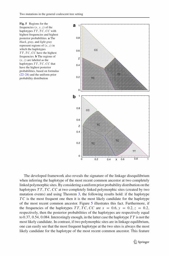
Fig. 5 Regions for thefrequencies (x, y, z) of thehaplotypes T T, T C,CC withhighest frequencies and highestposterior probabilities. a Theblack, gray, and light grayrepresent regions of (x, z) inwhich the haplotypesT T, T C,CC have the highestfrequencies. b The regions of(x, z) are labeled as thehaplotypes T T, T C,CC thathave the highest posteriorprobabilities, based on formulas(22–24) and the uniform priorprobability distribution
TC
CC
TT
TTTC
CC
Z
X
1
0.2
0
0.4
0.6
0.8
1
0.8
0.6
0.4
0.2
010.80.60.40.20
Z
a
b
TC
TC
The developed framework also reveals the signature of the linkage disequilibriumwhen inferring the haplotype of the most recent common ancestor at two completelylinked polymorphic sites. By considering a uniform prior probability distribution on thehaplotypes T T, T C,CC at two completely linked polymorphic sites (created by twomutation events) and using Theorem 3, the following results hold: if the haplotypeT C is the most frequent one then it is the most likely candidate for the haplotypeof the most recent common ancestor. Figure 5 illustrates this fact. Furthermore, ifthe frequencies of the haplotypes T T, T C,CC are x = 0.6, y = 0.2, z = 0.2,respectively, then the posterior probabilities of the haplotypes are respectively equalto 0.37, 0.54, 0.084. Interestingly enough, in the latter case the haplotype T T is not themost likely candidate. In contrast, if two polymorphic sites are in linkage equilibrium,one can easily see that the most frequent haplotype at the two sites is always the mostlikely candidate for the haplotype of the most recent common ancestor. This feature
123
O. Sargsyan
can be shown in the standard coalescent setting as well as in the general coalescent treesetting by using the frameworks developed by Kimura and Ohta (1973) and Sargsyanand Wakeley (2008), respectively. In these frameworks they have shown that the mostfrequent haplotype at a nucleotide site created by a single mutation is always the mostlikely candidate for the ancestral haplotype.
The signature of linkage disequilibrium is also present in the estimates of the ages ofthe two mutation events. I estimated the ages of the two mutation events for the APOEdata using the developed framework and applying the formula of Kimura and Ohta(1973) for each of the polymorphic sites. Table 3 shows that the estimates of the ages ofthe early mutation events are quite close under both methods, but the estimates of theages of the late mutation events differ approximately 2 times. Note that inconsistenciesbetween the ages of the early and late mutation events under both methods are moreobvious for the case of haplotype frequency data x = 0.6, y = 0.2, z = 0.2 (detailsnot shown).
The application of the framework to the APOE data under various demographicmodels (Table 2) suggests that e3(T C) is more likely to be the haplotype for themost recent common ancestor of modern human populations instead of the haplotypeCC carried by the non-human primates. As the framework shows this inference is aconsequence of the fact that the haplotype e3 is the most frequent one in modern humanpopulations. Selection forces might have contributed to the increase of the frequencyof e3 (Corbo and Scacchi 1999). Further studies are needed to explore the impact ofselection forces as well as other prior probability distributions for the haplotypes onthe inference.
Acknowledgments I would like to thank Professor Simon Tavaré for his advice on the early stage of thiswork and Professor John Wakeley for helpful discussion on the early version of this manuscript. I wouldlike also to thank the two anonymous reviewers for their comments and suggestions for improving thepresentation of the manuscript.
Appendix
The proof of Lemma 1
I first derive expressions for the numbers N1(k,m; b, c, a) and N2(k,m; a, c, b)when a, b, c are positive. In the derivations I use an additional condition that the thesequences in the sample are labeled and in a particular order. To remove this condition
for completing the proof, the derived numbers must be multiplied by
(a + b + c
a b c
)
.
Since N1(k,m; b, c, a) represents possible topologies of the genealogies with twomutations that are consistent with the data (a, b, c) when the ancestral haplotype atthe two sites is T T, transition history at early and late mutation events is H1 =(T T → T C → CC), and the number of ancestral lineages at the early and latemutation events are k and m, respectively; from the definition of (k,m) follows that3 ≤ m ≤ b + a + 1, k is less than or equal to m − 1, and 2 ≤ k ≤ a + 1, consequently2 ≤ k ≤ min(a + 1,m − 1).
123
Two mutations in the general coalescent tree setting
The genealogies satisfying the above conditions can be represented as a combinationof three parts determined by the early and late mutation events. The first part of thegenealogy is between sampling time point and the late mutation event; the second partis the part of the genealogy between the late and early mutation events; the third partis between the early mutation event and the time of the most recent common ancestorof the sample. The numbers of possible topologies in the three parts of the genealogydetermine N1(k,m; b, c, a).
For this purpose I consider the sample as combination of three groups of sequencesdetermined by the haplotypes T T, T C,CC. In the first part of the genealogy thelineages coalesce only with the lineages of their groups, in other words the groupsdo not share an ancestor up to the time of the late mutation event. At this time pointthe number of the lineages associated with the group CC is 1. Let the numbers ofthe lineages for the groups of T C and T T label by m1 and m2, respectively. Thenumber of topologies of the genealogies conditioned on {m1,m2}, is a product of thenumbers of possible topologies in the three parts of the genealogy. I provide in detailsthe derivation of the number of possible topologies in the first part of the genealogy.
The coalescent events occur one at a time in consecutive order back in time, andthe total number of such events on this part of the genealogy is a + b + c − m. Thesecoalescent events are distributed among the genealogies of the groups CC, T C , andT T as c − 1, b − m1, and a − m2, respectively. Consequently, the number of ways ofdistributing the coalescent events for the groups is
(a + b + c − m
c − 1, b − m1, a − m2
)
.
For a given sequence of the coalescent events among the groups, the topologies of thegenealogies of the groups have random joining structure, therefore the numbers of thepossible topologies of the genealogies of the groups T T, T C,CC are computed basedon the following formula: If i lineages are traced back in time and stopped when thenumber of lineages is j by randomly joining two lineages at each coalescent event,the number of all possible generated topologies is equal to
γ (i, j) ≡(
i
2
)(i − 1
2
)
· · ·(
j + 1
2
)
, j ≤ i − 1.
From this observation follows that the number of all possible topologies for the firstpart of the genealogy conditional on {m1,m2}, is equal to
(a + b + c − m
c − 1, b − m1, a − m2
)
γ (c, 1)γ (b,m1)γ (a,m2).
The same type of approach one can use to compute the numbers of the topologiesfor the second and third parts of the genealogy (details not shown). These numbersare equal to
(m − k
m1
)
γ (m1 + 1, 1)γ (m2, k − 1)
123
O. Sargsyan
and
γ (k, 1),
respectively. Thus, after multiplying the above three expressions and simplifying theproduct, the following formula holds for the number of the topologies of the genealo-gies conditional on m1,m2:
N (a, b, c)
(m − m2
2
)(k
2
)(a + b + c − m
c − 1
)(a + b + 1 − m
a − m2
)(m − k
m2 − k + 1
)
,
where
N (a, b, c) ≡ a!(a − 1)!2a−1
b!(b − 1)!2b−1
c!(c − 1)!2c−1 .
From the definition of m1 and m2, the following inequalities hold
m1 + m2 + 1 = m, 1 ≤ m1 ≤ b, 1 ≤ m2 ≤ a, and 2 ≤ k ≤ m2 + 1,
and from these conditions follows that m2 satisfies
m − b − 1 ≤ m2 ≤ m − 2,
and
max(m − b − 1, 1) ≤ m2 ≤ min(m − 2, a),
consequentlymax(m − b − 1, k − 1) ≤ m2 ≤ min(m − 2, a). (33)
From the above derivations and the boundary conditions in (33) follows that thelabeled and particularly ordered version of N1(k,m; b, c, a) can be represented as thesum
N (a, b, c)
(a + b + c − m
c − 1
)(k
2
)
×min(a,m−2)∑
m2=max(k−1,m−b−1)
(m − m2)(m − m2 − 1)
2
(a + b + 1 − m
a − m2
)(m − k
m2 − k + 1
)
(34)
Note that changing the range for m2 in the above sum to max(k−1,m−b−1) ≤ m2 ≤min(a,m − 1) does not change the result of the sum because the term correspondingto m2 = m − 1 is zero.
123
Two mutations in the general coalescent tree setting
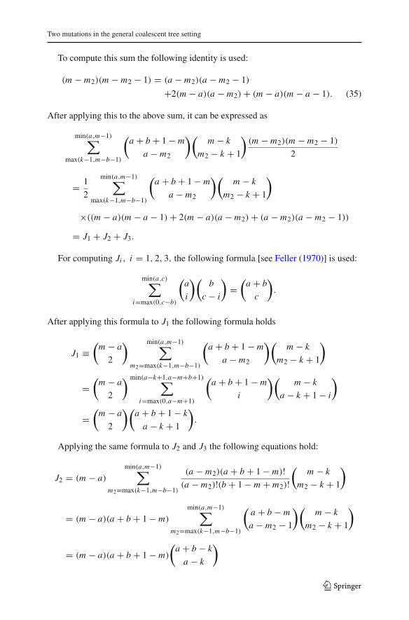
To compute this sum the following identity is used:
(m − m2)(m − m2 − 1) = (a − m2)(a − m2 − 1)
+2(m − a)(a − m2)+ (m − a)(m − a − 1). (35)
After applying this to the above sum, it can be expressed as
min(a,m−1)∑
max(k−1,m−b−1)
(a + b + 1 − m
a − m2
)(m − k
m2 − k + 1
)(m − m2)(m − m2 − 1)
2
= 1
2
min(a,m−1)∑
max(k−1,m−b−1)
(a + b + 1 − m
a − m2
)(m − k
m2 − k + 1
)
×((m − a)(m − a − 1)+ 2(m − a)(a − m2)+ (a − m2)(a − m2 − 1))
= J1 + J2 + J3.
For computing Ji , i = 1, 2, 3, the following formula [see Feller (1970)] is used:
min(a,c)∑
i=max(0,c−b)
(a
i
)(b
c − i
)
=(
a + b
c
)
.
After applying this formula to J1 the following formula holds
J1 ≡(
m − a
2
) min(a,m−1)∑
m2=max(k−1,m−b−1)
(a + b + 1 − m
a − m2
)(m − k
m2 − k + 1
)
=(
m − a
2
) min(a−k+1,a−m+b+1)∑
i=max(0,a−m+1)
(a + b + 1 − m
i
)(m − k
a − k + 1 − i
)
=(
m − a
2
)(a + b + 1 − k
a − k + 1
)
.
Applying the same formula to J2 and J3 the following equations hold:
J2 = (m − a)min(a,m−1)∑
m2=max(k−1,m−b−1)
(a − m2)(a + b + 1 − m)!(a − m2)!(b + 1 − m + m2)!
(m − k
m2 − k + 1
)
= (m − a)(a + b + 1 − m)min(a,m−1)∑
m2=max(k−1,m−b−1)
(a + b − m
a − m2 − 1
)(m − k
m2 − k + 1
)
= (m − a)(a + b + 1 − m)
(a + b − k
a − k
)
123
O. Sargsyan
and
J3 =min(a,m−1)∑
m2=max(k−1,m−b−1)
(a − m2
2
)(a + b + 1 − m
a − m2
)(m − k
m2 − k + 1
)
=(
a + b + 1 − m
2
) min(a,m−1)∑
m2=max(k−1,m−b−1)
(a + b − k − 1
a − m2 − 2
)(m − k
m2 − k + 1
)
= 1
2(a + b + 1 − m)(a + b − m)
(a + b − k − 1
a − k − 1
)
.
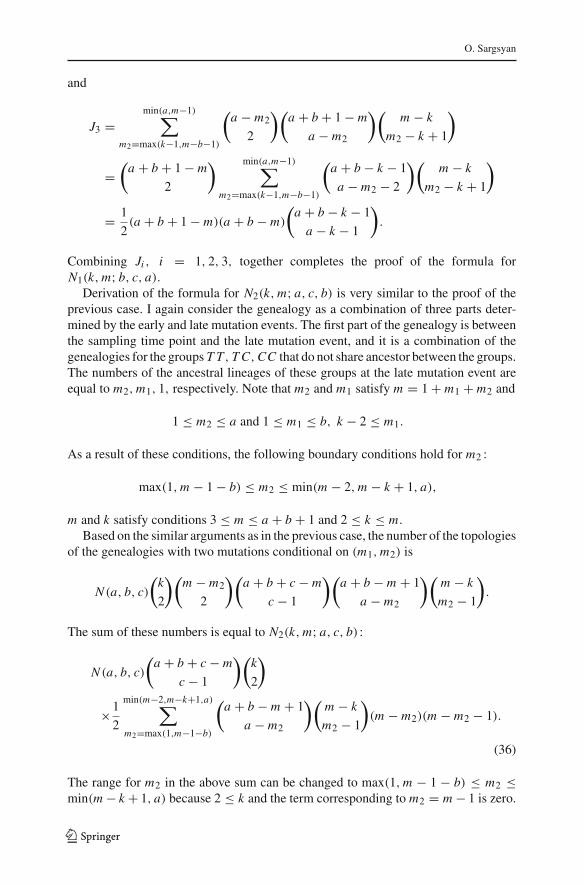
Combining Ji , i = 1, 2, 3, together completes the proof of the formula forN1(k,m; b, c, a).
Derivation of the formula for N2(k,m; a, c, b) is very similar to the proof of theprevious case. I again consider the genealogy as a combination of three parts deter-mined by the early and late mutation events. The first part of the genealogy is betweenthe sampling time point and the late mutation event, and it is a combination of thegenealogies for the groups T T, T C,CC that do not share ancestor between the groups.The numbers of the ancestral lineages of these groups at the late mutation event areequal to m2,m1, 1, respectively. Note that m2 and m1 satisfy m = 1 + m1 + m2 and
1 ≤ m2 ≤ a and 1 ≤ m1 ≤ b, k − 2 ≤ m1.
As a result of these conditions, the following boundary conditions hold for m2 :
max(1,m − 1 − b) ≤ m2 ≤ min(m − 2,m − k + 1, a),
m and k satisfy conditions 3 ≤ m ≤ a + b + 1 and 2 ≤ k ≤ m.Based on the similar arguments as in the previous case, the number of the topologies
of the genealogies with two mutations conditional on (m1,m2) is
N (a, b, c)
(k
2
)(m − m2
2
)(a + b + c − m
c − 1
)(a + b − m + 1
a − m2
)(m − k
m2 − 1
)
.
The sum of these numbers is equal to N2(k,m; a, c, b) :
N (a, b, c)
(a + b + c − m
c − 1
)(k
2
)
×1
2
min(m−2,m−k+1,a)∑
m2=max(1,m−1−b)
(a + b − m + 1
a − m2
)(m − k
m2 − 1
)
(m − m2)(m − m2 − 1).
(36)
The range for m2 in the above sum can be changed to max(1,m − 1 − b) ≤ m2 ≤min(m − k + 1, a) because 2 ≤ k and the term corresponding to m2 = m − 1 is zero.
123
Two mutations in the general coalescent tree setting
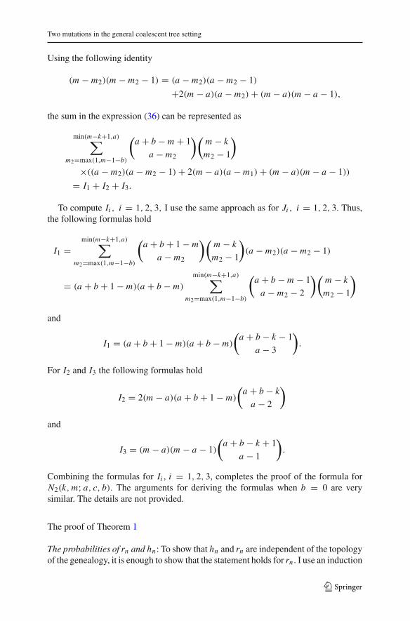
Using the following identity
(m − m2)(m − m2 − 1) = (a − m2)(a − m2 − 1)
+2(m − a)(a − m2)+ (m − a)(m − a − 1),
the sum in the expression (36) can be represented as
min(m−k+1,a)∑
m2=max(1,m−1−b)
(a + b − m + 1
a − m2
)(m − k
m2 − 1
)
×((a − m2)(a − m2 − 1)+ 2(m − a)(a − m1)+ (m − a)(m − a − 1))
= I1 + I2 + I3.
To compute Ii , i = 1, 2, 3, I use the same approach as for Ji , i = 1, 2, 3. Thus,the following formulas hold
I1 =min(m−k+1,a)∑
m2=max(1,m−1−b)
(a + b + 1 − m
a − m2
)(m − k
m2 − 1
)
(a − m2)(a − m2 − 1)
= (a + b + 1 − m)(a + b − m)min(m−k+1,a)∑
m2=max(1,m−1−b)
(a + b − m − 1
a − m2 − 2
)(m − k
m2 − 1
)
and
I1 = (a + b + 1 − m)(a + b − m)
(a + b − k − 1
a − 3
)
.
For I2 and I3 the following formulas hold
I2 = 2(m − a)(a + b + 1 − m)
(a + b − k
a − 2
)
and
I3 = (m − a)(m − a − 1)
(a + b − k + 1
a − 1
)
.
Combining the formulas for Ii , i = 1, 2, 3, completes the proof of the formula forN2(k,m; a, c, b). The arguments for deriving the formulas when b = 0 are verysimilar. The details are not provided.
The proof of Theorem 1
The probabilities of rn and hn : To show that hn and rn are independent of the topologyof the genealogy, it is enough to show that the statement holds for rn . I use an induction
123
O. Sargsyan
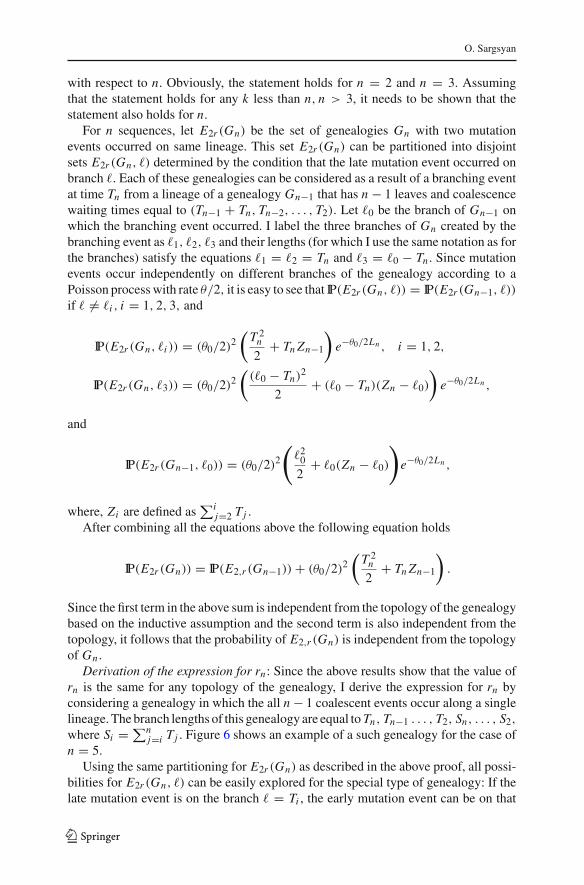
with respect to n. Obviously, the statement holds for n = 2 and n = 3. Assumingthat the statement holds for any k less than n, n > 3, it needs to be shown that thestatement also holds for n.
For n sequences, let E2r (Gn) be the set of genealogies Gn with two mutationevents occurred on same lineage. This set E2r (Gn) can be partitioned into disjointsets E2r (Gn, ) determined by the condition that the late mutation event occurred onbranch . Each of these genealogies can be considered as a result of a branching eventat time Tn from a lineage of a genealogy Gn−1 that has n − 1 leaves and coalescencewaiting times equal to (Tn−1 + Tn, Tn−2, . . . , T2). Let 0 be the branch of Gn−1 onwhich the branching event occurred. I label the three branches of Gn created by thebranching event as 1, 2, 3 and their lengths (for which I use the same notation as forthe branches) satisfy the equations 1 = 2 = Tn and 3 = 0 − Tn . Since mutationevents occur independently on different branches of the genealogy according to aPoisson process with rate θ/2, it is easy to see that IP(E2r (Gn, )) = IP(E2r (Gn−1, ))
if �= i , i = 1, 2, 3, and
IP(E2r (Gn, i )) = (θ0/2)2(
T 2n
2+ Tn Zn−1
)
e−θ0/2Ln , i = 1, 2,
IP(E2r (Gn, 3)) = (θ0/2)2(( 0 − Tn)
2
2+ ( 0 − Tn)(Zn − 0)
)
e−θ0/2Ln ,
and
IP(E2r (Gn−1, 0)) = (θ0/2)2
( 2
0
2+ 0(Zn − 0)
)
e−θ0/2Ln ,
where, Zi are defined as∑i
j=2 Tj .
After combining all the equations above the following equation holds
IP(E2r (Gn)) = IP(E2,r (Gn−1))+ (θ0/2)2(
T 2n
2+ Tn Zn−1
)
.
Since the first term in the above sum is independent from the topology of the genealogybased on the inductive assumption and the second term is also independent from thetopology, it follows that the probability of E2,r (Gn) is independent from the topologyof Gn .
Derivation of the expression for rn : Since the above results show that the value ofrn is the same for any topology of the genealogy, I derive the expression for rn byconsidering a genealogy in which the all n − 1 coalescent events occur along a singlelineage. The branch lengths of this genealogy are equal to Tn, Tn−1 . . . , T2, Sn, . . . , S2,
where Si = ∑nj=i Tj . Figure 6 shows an example of a such genealogy for the case of
n = 5.Using the same partitioning for E2r (Gn) as described in the above proof, all possi-
bilities for E2r (Gn, ) can be easily explored for the special type of genealogy: If thelate mutation event is on the branch = Ti , the early mutation event can be on that
123
Two mutations in the general coalescent tree setting
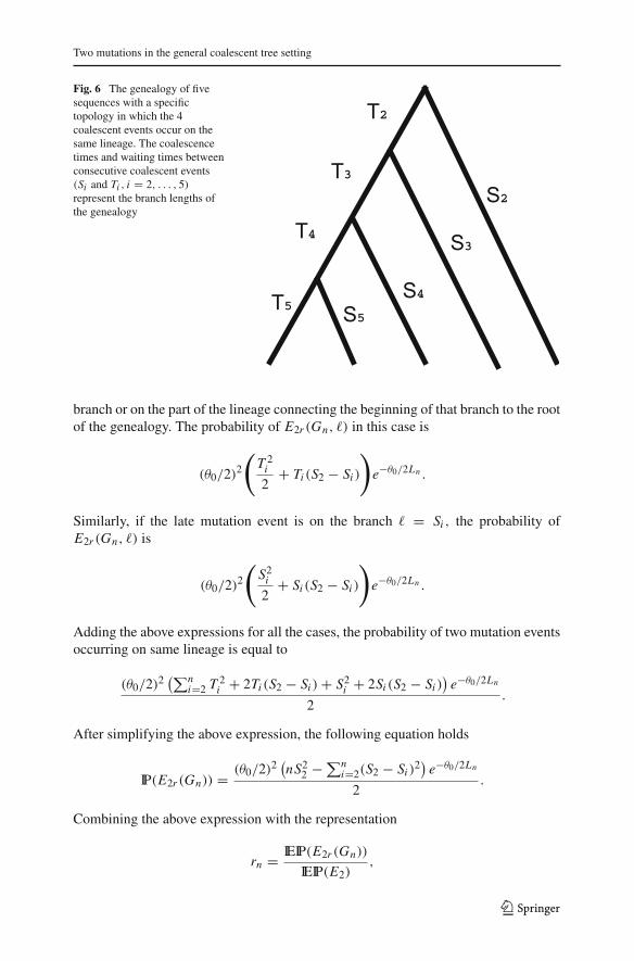
Fig. 6 The genealogy of fivesequences with a specifictopology in which the 4coalescent events occur on thesame lineage. The coalescencetimes and waiting times betweenconsecutive coalescent events(Si and Ti , i = 2, . . . , 5)represent the branch lengths ofthe genealogy
branch or on the part of the lineage connecting the beginning of that branch to the rootof the genealogy. The probability of E2r (Gn, ) in this case is
(θ0/2)2
(T 2
i
2+ Ti (S2 − Si )
)
e−θ0/2Ln .
Similarly, if the late mutation event is on the branch = Si , the probability ofE2r (Gn, ) is
(θ0/2)2
(S2
i
2+ Si (S2 − Si )
)
e−θ0/2Ln .
Adding the above expressions for all the cases, the probability of two mutation eventsoccurring on same lineage is equal to
(θ0/2)2(∑n
i=2 T 2i + 2Ti (S2 − Si )+ S2
i + 2Si (S2 − Si ))
e−θ0/2Ln
2.
After simplifying the above expression, the following equation holds
IP(E2r (Gn)) = (θ0/2)2(nS2
2 − ∑ni=2(S2 − Si )
2)
e−θ0/2Ln
2.
Combining the above expression with the representation
rn = IEIP(E2r (Gn))
IEIP(E2),
123
O. Sargsyan
the following formula holds
rn = IE((nS2
2 − ∑ni=2(S2 − Si )
2)e−θ0 Ln/2)
IE(L2ne−θ0 Ln/2)
.
The proof of the inequality hn > rn, n > 2: I use a mathematical induction to provethat hn −rn > 0 if n > 2. From the previous results follows that the difference hn −rn
can be represented as
hn − rn = IE((L2
n − 2nS22 + 2
∑ni=2(S2 − Si )
2)e−θ0 Ln/2)
IE(L2ne−θ0 Ln/2)
. (37)
The following notations are needed Zi = ∑ij=2 Tj andφn = L2
n−2nZ2n+2
∑n−1i=2 Z2
i ,
which is equal to L2n − 2nS2
2 + 2∑n
i=2(S2 − Si )2. For n = 3, it is easy to check that
φ3 = L23 − 6Z2
3 + 2Z22 = 3T 2
3 > 0.
Assume that φk > 0 if k = n −1, I prove that this inequality also holds if k = n. SinceLn = ∑n
j=2 jTj , it can be represented as nTn + Ln−1 as well as nZn − ∑n−1i=2 Zi .
Thus, the following formula holds
φn − φn−1 = n(n − 2)T 2n + 2nTn
(
(n − 3)Zn−1 −n−2∑
i=2
Zi
)
.
As a result, the inequality
φn > 0.
holds since φn−1 is greater than 0 and
(n − 3)Zn−1 −n−2∑
i=2
Zi > 0.
Derivations of the formulas for IP(E2r,s | E2) and IP(E2h,c | E2): I derive theformulas using the following representations for the probabilities IP(E2r,s | E2) andIP(E2h,c | E2) :
IP(E2r,s | E2) =n∑
a=1
IP ((a, 0, n − a) | T T, H1, E2)
and
IP(E2h,c | E2) =n∑
a=1
IP ((a, 0, n − a) | T C, H2, E2) ,
123
Two mutations in the general coalescent tree setting
which I modify based on the Eq. (9) and changing the orders of the terms in sums.Thus, the following equations hold
IP(E2r,s | E2)
=∑n
m=2∑m
k=2
(∑n−1a=m−1 N1(k,m; 0, n − a, a)
)dm,kIE(Tk Tme−θ0 Ln/2)
N (n)IE((L2
n/2)e−θ0 Ln/2
)
and
IP(E2h,c | E2) =∑n
m=2
(∑n−1a=m−1 N2(k,m; a, n − a, 0)
)dm,kIE(Tk Tme−θ0 Ln/2)
N (n)IE((L2
n/2)e−θ0 Ln/2
) .
The above sums I simplify further using the formulas for N1() and N2() and the identity
w∑
r=v
(r
v
)
=(w + 1
v + 1
)
.
Hence, the following formulas hold
n−1∑
a=m−1
N1(k,m; 0, n − a, a)
N (n)= k(k − 1)(n − m)!(m − 2)!
(n − 1)!n−1∑
a=m−1
(a − 1
m − 2
)
= k(k − 1)
m − 1
and
n−1∑
a=m−1
N2(k,m; a, n − a, 0)
N (n)= 2(m − 2)!(n − m)!
(n − 1)!n−1∑
a=m−1
(a − 1
m − 2
)
= 2
m − 1.
The proof of Theorem 1 is complete.
The proof of Theorem 2
I represent the probability IP(Dn | α, Hα, E2) as a ratio of probabilities:
IP(Dn | α, Hα, E2) = IP(Dn, α, Hα, E2)
IP(α, Hα, E2).
To derive expressions for the probabilities in the numerator and denominator, I usethe framework for generating polymorphisms in samples of DNA sequences in thegeneral coalescent tree setting. The coalescence waiting times are determined by therandom variables Tn, . . . , T2, and mutation events are added along the lineages of the
123
O. Sargsyan
genealogy according to a Poisson process with rate θ0/2. Because of these properties,the probability in the denominator can be represented as
IP(α, Hα, E2) = IP(α, Hα)IE((θ20 L2
n/8)e−θ0 Ln/2),
where Ln is the total branch length of the genealogy. Using a similar approachdescribed by Sargsyan (2010), the probability in the numerator can be representedas the sum
IP(Dn, α, Hα, E2) =∑
(k,m)∈Δ j (e)
IEIP(Γ (k,m) ∼= Dn | Γ (k,m)),
where Γ (k,m) represent genealogies with two mutation events satisfying the follow-ing conditions: (1) The number of ancestral lineages at the early and late mutationevents are k and m, respectively. (2) The α is the haplotype of the most recent com-mon ancestor, and Hα is the transition history at early and late mutation events. Thesymbol “∼=” means that the genealogy with two mutations is consistent with Dn . Eachterm of this sum can be represented as a sum based on the definition of the conditionalexpectation. Thus,
IEIP(Γ (k,m) ∼= Dn | Γ (k,m)) =∑
Γ (k,m)
IP(Γ (k,m) ∼= Dn | Γ (k,m))IP(Γ (k,m)),
where the probability of Γ (k,m) is equal to
IP(Γ (k,m)) = IP(α, Hα)dm,kθ0Tk
2
θ0Tm
2e−θ0 Ln/2
and
IP(Γ (k,m) ∼= Dn | Γ (k,m)) = N j (k,m; e)
N (n),
the values of j and e are determined by α, Hα and the frequencies (a, b, c) of thehaplotypes T T, T C,CC. The quantity N(n) represents the number of all possibletopological trees with n leaves and it is equal to = n!(n − 1!)/2n−1, which can beeasily derived based on tracing and joining two lineages at each coalescent event.Combining the above equations completes the proof.
123
Two mutations in the general coalescent tree setting
The proof of Lemma 2
First I derive the asymptotic formula when T T is the ancestral haplotype. Factoringout some of the terms in Eq. (7), the following holds
N1(k,m; b, c, a)
=(
a + b + c
a b c
)
N (a, b, c)
(a + b + c − m
c − 1
)k(k − 1)
2
(a + b − k − 1)!b!(a + 1 − k)!
×(
1
2(m − a)(m − a − 1)(a + b + 1 − k)(a + b − k)
+ (m − a)(a + b + 1 − m)(a + b − k)(a − k + 1)
+ 1
2(a + b + 1 − m)(a + b − m)(a − k + 1)(a − k)
)
.
and
N1(k,m; b, c, a)N (n)n2
= n24(a − 1)!(a + b + c − m)! k(k−1)2 (a + b − k − 1)!
(a + 1 − k)!(a + b + c − 1)!(a + b + 1 − m)!b(
1
2(m − a)(m − a − 1)(a + b + 1 − k)(a + b − k)
+(m − a)(a + b + 1 − m)(a + b − k)(a − k + 1)
+1
2(a + b + 1 − m)(a + b − m)(a − k + 1)(a − k)
)
.
To approximate this ratio under the limits a/n → x, b/n → y, c/n → z as a, b, ctend to ∞, first the following limit is derived
(a − 1)!(a + 1 − k)!(a + b + c)k−2 → xk−2,
which follows from the representation
(a − 1)!(a + 1 − k)!(a + b + c)k−2 = (a − k + 2)
(a + b + c)· · · (a − 1)
(a + b + c).
Using similar approach the following limits hold:
(a + b − k − 1)!(a + b + 1 − m)!(a + b + c)m−k−2 → (x + y)m−k−2,
and
(a + b + c − m)!(a + b + c)m−1
(a + b + c − 1)! → 1.
123
O. Sargsyan
After expanding the expression
(1
2(m − a)(m − a − 1)(a + b + 1 − k)(a + b − k)
+(m − a)(a + b + 1 − m)(a + b − k)(a − k + 1)
+1
2(a + b + 1 − m)(a + b − m)(a − k + 1)(a − k)
)
to
−bk
2− b2k
2− bak + bk2
2+ b2k2
2+ bm
2+ b2m
2+ bam − b2km − bm2
2+ b2m2
2,
it is asymptotically equal to (a+b+c)2 y2 (m−k)(2x+y(m−k+1))). After combining
these results the following limit holds
N1(k,m; b, c, a)N (n)n2
→ k(k − 1)(m − k)(2xk−1 + xk−2 y(m − k + 1))
(x + y)k−m+2 .
Note that the above approach can be applied similarly to derive the asymptotic formulafor N2(k,m; a, c, b). The proof of the lemma is complete.
The proof of Theorem 3
In the standard coalescent setting Ti , i = 2, . . . , n, are pairwise independent expo-nential random variables with rates 2/(i(i − 1)), therefore the following equationshold:
IE(Tk Tm) = 4
k(k − 1)m(m − 1), m �= k,
and
IE(T 2m) = 8
(m(m − 1))2.
Using these formulas and the approximations in Lemma 2, I compute the limit of theexpression
n2
N (n)
b+a+1∑
m=3
min(m−1,a+1)∑
k=2
N1(k,m; b, c, a)dm,kIE(Tk Tm)
under the conditions a/n → x, b/n → y, c/n → z as a, b, c tend to ∞, bysubstituting the ratio
123
Two mutations in the general coalescent tree setting
N1(k,m; b, c, a)N (n)n2
dm,kIE(Tk Tm)
with
D1(y, k; z,m)4
m(m − 1)k(k − 1)
and showing that the following identity holds
∞∑
m=3
m−1∑
k=2
D1(y, k; z,m)4
m(m − 1)k(k − 1)= F(z).
Similar to this approach the following equations hold for the other cases
∞∑
m=3
m∑
k=2
D2(x, k; z,m)4
m(m − 1)k(k − 1)=
(4
z(x + z)− F(z)
)
,
∞∑
m=3
m∑
k=2
D2(z, k; x,m)4
m(m − 1)k(k − 1)=
(4
x(x + z)− F(x)
)
.
Note that if m = k then
∞∑
m=3
D2(x,m; z,m)8
m2(m − 1)2= 2F(1 − y).
For the derivations of these formulas I used Wolfram Mathematica Software andthe formulas
∞∑
i=0
t i = 1
1 − t,
and
∞∑
i=1
t i
i= − log(1 − t).
Under the limits an → x, b
n → y, c/n → z, as a, b, c tend to ∞ the followinglimits hold in the standard coalescent setting:
n2
N (n)
b+a+1∑
m=3
min(m−1,a+1)∑
k=2
N1(k,m; b, c, a)dm,k IE(Tk Tm) → F(z),
123
O. Sargsyan
n2
N (n)
b+c+1∑
m=3
min(m−1,c+1)∑
k=2
N1(k,m; b, a, c)dm,k IE(Tk Tm) → F(x),
n2
N (n)
a+b+1∑
m=3
min(m,b+2)∑
k=2
N2(k,m; a, c, b)dm,k IE(Tk Tm) → Δ(z, x, y),
n2
N (n)
b+c+1∑
m=3
min(m,b+2)∑
k=2
N2(k,m; c, a, b)dm,k IE(Tk Tm) → Δ(x, z, y),
where
Δ(z, x, y) ≡(
4
z(x + z)− F(z)
)
and
F(x) ≡ 4(1 − x2 + 2x log(x))
x(1 − x)3.
Based on Eq. (6) and (17) the following holds
IP(T T | (x, y, z), E2) ∝ IP((x, y, z) | T T, H1, E2)πT T ,
IP(T C | (x, y, z), E2) ∝ (IP((x, y, z) | TC, H2, E2)+IP((x, y, z) | TC, H3, E2))πT C ,
IP(CC | (x, y, z), E2) ∝ IP((x, y, z) | CC, H4, E2)πCC .
Combining these equations with the above limits the proof of the theorem is complete.
The proof of Theorem 4
Derivations here are very similar to the approach used by Sargsyan (2010), for moredetails see that paper. First I represent the joint distribution of the ages of ξ1, ξ2, andξ as the ratio of two probabilities:
IP(ξ1 ≤ t1, ξ2 ≤ t2, ξ ≤ t | Dn, α, Hα, E2)
= IP(ξ1 ≤ t1, ξ2 ≤ t2, ξ ≤ t, Dn, α, Hα, E2)
IP(Dn, α, Hα, E2).
The denominator in the above equation can be substituted by the expression inTheorem 2. To derive an expression for the probability in the numerator one canuse very similar approach as in Theorem 2. After determining j and e based on α, Hαand (a, b, c) (the frequencies of the haplotypes T T, T C,CC) the following equation
123
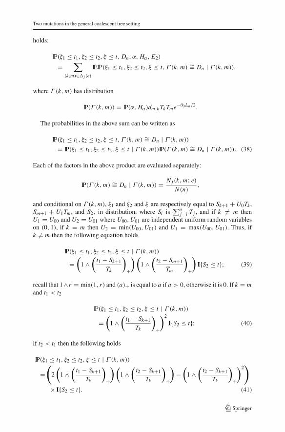
Two mutations in the general coalescent tree setting
holds:
IP(ξ1 ≤ t1, ξ2 ≤ t2, ξ ≤ t, Dn, α, Hα, E2)
=∑
(k,m)∈Δ j (e)
IEIP(ξ1 ≤ t1, ξ2 ≤ t2, ξ ≤ t, Γ (k,m) ∼= Dn | Γ (k,m)),
where Γ (k,m) has distribution
IP(Γ (k,m)) = IP(α, Hα)dm,k Tk Tme−θ0 Ln/2.
The probabilities in the above sum can be written as
IP(ξ1 ≤ t1, ξ2 ≤ t2, ξ ≤ t, Γ (k,m) ∼= Dn | Γ (k,m))
= IP(ξ1 ≤ t1, ξ2 ≤ t2, ξ ≤ t | Γ (k,m))IP(Γ (k,m) ∼= Dn | Γ (k,m)). (38)
Each of the factors in the above product are evaluated separately:
IP(Γ (k,m) ∼= Dn | Γ (k,m)) = N j (k,m; e)
N (n),
and conditional on Γ (k,m), ξ1 and ξ2 and ξ are respectively equal to Sk+1 + U0Tk ,Sm+1 + U1Tm , and S2, in distribution, where Si is
∑nj=i Tj , and if k �= m then
U1 = U00 and U2 = U01 where U00,U01 are independent uniform random variableson (0, 1), if k = m then U2 = min(U00,U01) and U1 = max(U00,U01). Thus, ifk �= m then the following equation holds
IP(ξ1 ≤ t1, ξ2 ≤ t2, ξ ≤ t | Γ (k,m))
=(
1 ∧(
t1 − Sk+1
Tk
)
+
) (
1 ∧(
t2 − Sm+1
Tm
)
+
)
I{S2 ≤ t}; (39)
recall that 1∧r = min(1, r) and (a)+ is equal to a if a > 0, otherwise it is 0. If k = mand t1 < t2
IP(ξ1 ≤ t1, ξ2 ≤ t2, ξ ≤ t | Γ (k,m))
=(
1 ∧(
t1 − Sk+1
Tk
)
+
)2
I{S2 ≤ t}; (40)
if t2 < t1 then the following holds
IP(ξ1 ≤ t1, ξ2 ≤ t2, ξ ≤ t | Γ (k,m))
=(
2
(
1 ∧(
t1 − Sk+1
Tk
)
+
) (
1 ∧(
t2 − Sk+1
Tk
)
+
)
−(
1 ∧(
t2 − Sk+1
Tk
)
+
)2)
× I{S2 ≤ t}. (41)
123
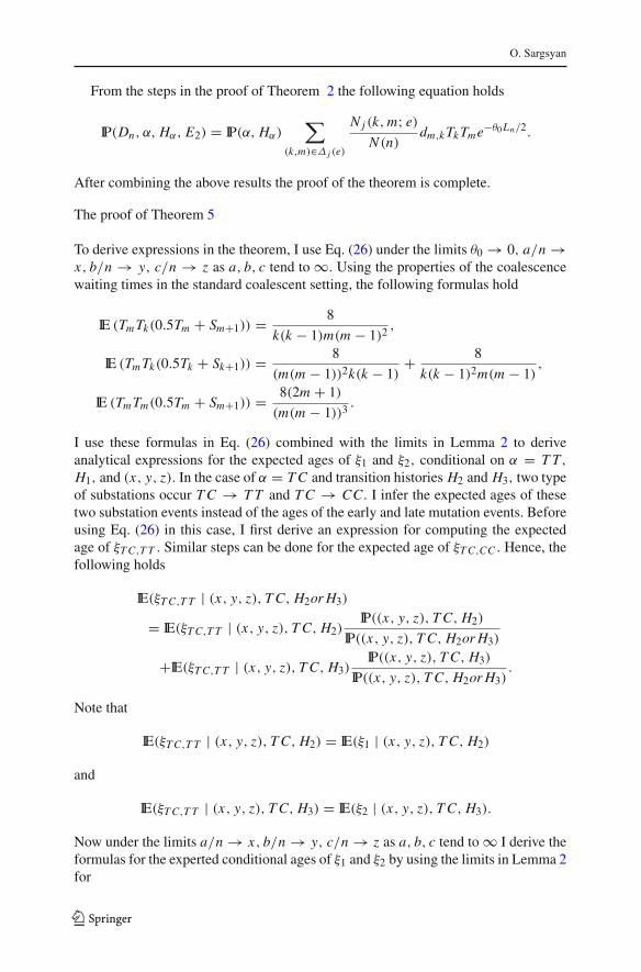
O. Sargsyan
From the steps in the proof of Theorem 2 the following equation holds
IP(Dn, α, Hα, E2) = IP(α, Hα)∑
(k,m)∈Δ j (e)
N j (k,m; e)
N (n)dm,k Tk Tme−θ0 Ln/2.
After combining the above results the proof of the theorem is complete.
The proof of Theorem 5
To derive expressions in the theorem, I use Eq. (26) under the limits θ0 → 0, a/n →x, b/n → y, c/n → z as a, b, c tend to ∞. Using the properties of the coalescencewaiting times in the standard coalescent setting, the following formulas hold
IE (Tm Tk(0.5Tm + Sm+1)) = 8
k(k − 1)m(m − 1)2,
IE (Tm Tk(0.5Tk + Sk+1)) = 8
(m(m − 1))2k(k − 1)+ 8
k(k − 1)2m(m − 1),
IE (Tm Tm(0.5Tm + Sm+1)) = 8(2m + 1)
(m(m − 1))3.
I use these formulas in Eq. (26) combined with the limits in Lemma 2 to deriveanalytical expressions for the expected ages of ξ1 and ξ2, conditional on α = T T,H1, and (x, y, z). In the case of α = T C and transition histories H2 and H3, two typeof substations occur T C → T T and T C → CC. I infer the expected ages of thesetwo substation events instead of the ages of the early and late mutation events. Beforeusing Eq. (26) in this case, I first derive an expression for computing the expectedage of ξT C,T T . Similar steps can be done for the expected age of ξT C,CC . Hence, thefollowing holds
IE(ξT C,T T | (x, y, z), T C, H2or H3)
= IE(ξT C,T T | (x, y, z), T C, H2)IP((x, y, z), T C, H2)
IP((x, y, z), T C, H2or H3)
+IE(ξT C,T T | (x, y, z), T C, H3)IP((x, y, z), T C, H3)
IP((x, y, z), T C, H2or H3).
Note that
IE(ξT C,T T | (x, y, z), T C, H2) = IE(ξ1 | (x, y, z), T C, H2)
and
IE(ξT C,T T | (x, y, z), T C, H3) = IE(ξ2 | (x, y, z), T C, H3).
Now under the limits a/n → x, b/n → y, c/n → z as a, b, c tend to ∞ I derive theformulas for the experted conditional ages of ξ1 and ξ2 by using the limits in Lemma 2for
123
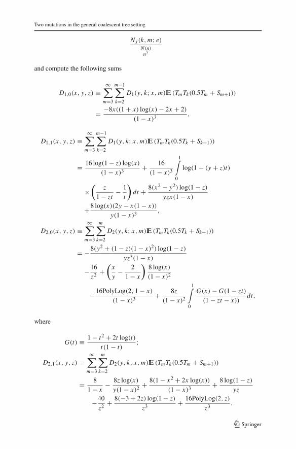
Two mutations in the general coalescent tree setting
N j (k,m; e)N (n)n2
and compute the following sums
D1,0(x, y, z) ≡∞∑
m=3
m−1∑
k=2
D1(y, k; x,m)IE (Tm Tk(0.5Tm + Sm+1))
= −8x((1 + x) log(x)− 2x + 2)
(1 − x)3,
D1,1(x, y, z) ≡∞∑
m=3
m−1∑
k=2
D1(y, k; x,m)IE (Tm Tk(0.5Tk + Sk+1))
= 16 log(1 − z) log(x)
(1 − x)3+ 16
(1 − x)3
1∫
0
log(1 − (y + z)t)
×(
z
1 − zt− 1
t
)
dt + 8(x2 − y2) log(1 − z)
yzx(1 − x)
+8 log(x)(2y − x(1 − x))
y(1 − x)3,
D2,0(x, y, z) ≡∞∑
m=3
m∑
k=2
D2(y, k; x,m)IE (Tm Tk(0.5Tk + Sk+1))
= −8(y2 + (1 − z)(1 − x)2) log(1 − z)
yz3(1 − x)
−16
z2 +(
x
y− 2
1 − x
)8 log(x)
(1 − x)2
−16PolyLog(2, 1 − x)
(1 − x)3+ 8z
(1 − x)2
1∫
0
G(x)− G(1 − zt)
(1 − zt − x))dt,
where
G(t) ≡ 1 − t2 + 2t log(t)
t (1 − t);
D2,1(x, y, z) ≡∞∑
m=3
m∑
k=2
D2(y, k; x,m)IE (Tm Tk(0.5Tm + Sm+1))
= 8
1 − x− 8z log(x)
y(1 − x)2+ 8(1 − x2 + 2x log(x))
(1 − x)3+ 8 log(1 − z)
yz
−40
z2 + 8(−3 + 2z) log(1 − z)
z3 + 16PolyLog(2, z)
z3 .
123
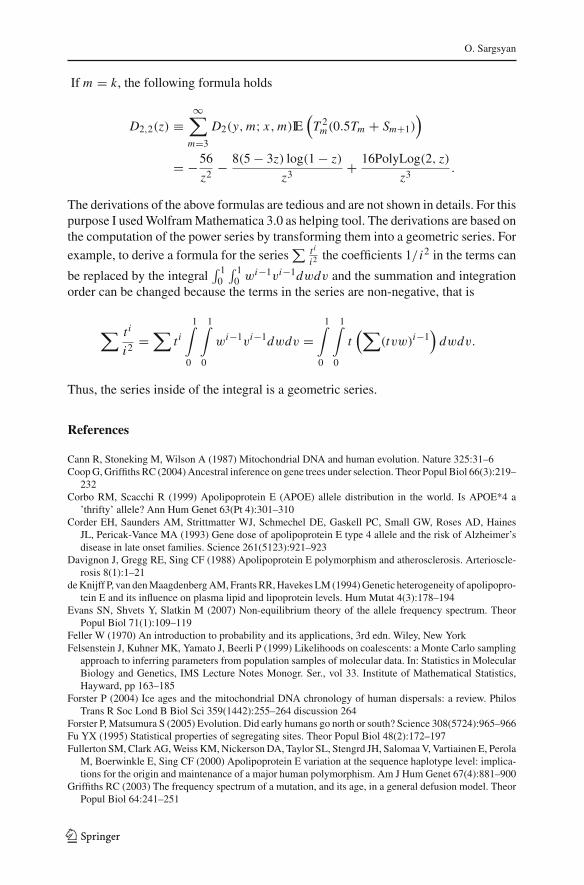
O. Sargsyan
If m = k, the following formula holds
D2,2(z) ≡∞∑
m=3
D2(y,m; x,m)IE(
T 2m(0.5Tm + Sm+1)
)
= −56
z2 − 8(5 − 3z) log(1 − z)
z3 + 16PolyLog(2, z)
z3 .
The derivations of the above formulas are tedious and are not shown in details. For thispurpose I used Wolfram Mathematica 3.0 as helping tool. The derivations are based onthe computation of the power series by transforming them into a geometric series. For
example, to derive a formula for the series∑ t i
i2 the coefficients 1/ i2 in the terms can
be replaced by the integral∫ 1
0
∫ 10 w
i−1vi−1dwdv and the summation and integrationorder can be changed because the terms in the series are non-negative, that is
∑ t i
i2 =∑
t i
1∫
0
1∫
0
wi−1vi−1dwdv =1∫
0
1∫
0
t(∑
(tvw)i−1)
dwdv.
Thus, the series inside of the integral is a geometric series.
References
Cann R, Stoneking M, Wilson A (1987) Mitochondrial DNA and human evolution. Nature 325:31–6Coop G, Griffiths RC (2004) Ancestral inference on gene trees under selection. Theor Popul Biol 66(3):219–
232Corbo RM, Scacchi R (1999) Apolipoprotein E (APOE) allele distribution in the world. Is APOE*4 a
’thrifty’ allele? Ann Hum Genet 63(Pt 4):301–310Corder EH, Saunders AM, Strittmatter WJ, Schmechel DE, Gaskell PC, Small GW, Roses AD, Haines
JL, Pericak-Vance MA (1993) Gene dose of apolipoprotein E type 4 allele and the risk of Alzheimer’sdisease in late onset families. Science 261(5123):921–923
Davignon J, Gregg RE, Sing CF (1988) Apolipoprotein E polymorphism and atherosclerosis. Arterioscle-rosis 8(1):1–21
de Knijff P, van den Maagdenberg AM, Frants RR, Havekes LM (1994) Genetic heterogeneity of apolipopro-tein E and its influence on plasma lipid and lipoprotein levels. Hum Mutat 4(3):178–194
Evans SN, Shvets Y, Slatkin M (2007) Non-equilibrium theory of the allele frequency spectrum. TheorPopul Biol 71(1):109–119
Feller W (1970) An introduction to probability and its applications, 3rd edn. Wiley, New YorkFelsenstein J, Kuhner MK, Yamato J, Beerli P (1999) Likelihoods on coalescents: a Monte Carlo sampling
approach to inferring parameters from population samples of molecular data. In: Statistics in MolecularBiology and Genetics, IMS Lecture Notes Monogr. Ser., vol 33. Institute of Mathematical Statistics,Hayward, pp 163–185
Forster P (2004) Ice ages and the mitochondrial DNA chronology of human dispersals: a review. PhilosTrans R Soc Lond B Biol Sci 359(1442):255–264 discussion 264
Forster P, Matsumura S (2005) Evolution. Did early humans go north or south? Science 308(5724):965–966Fu YX (1995) Statistical properties of segregating sites. Theor Popul Biol 48(2):172–197Fullerton SM, Clark AG, Weiss KM, Nickerson DA, Taylor SL, Stengrd JH, Salomaa V, Vartiainen E, Perola
M, Boerwinkle E, Sing CF (2000) Apolipoprotein E variation at the sequence haplotype level: implica-tions for the origin and maintenance of a major human polymorphism. Am J Hum Genet 67(4):881–900
Griffiths RC (2003) The frequency spectrum of a mutation, and its age, in a general defusion model. TheorPopul Biol 64:241–251
123
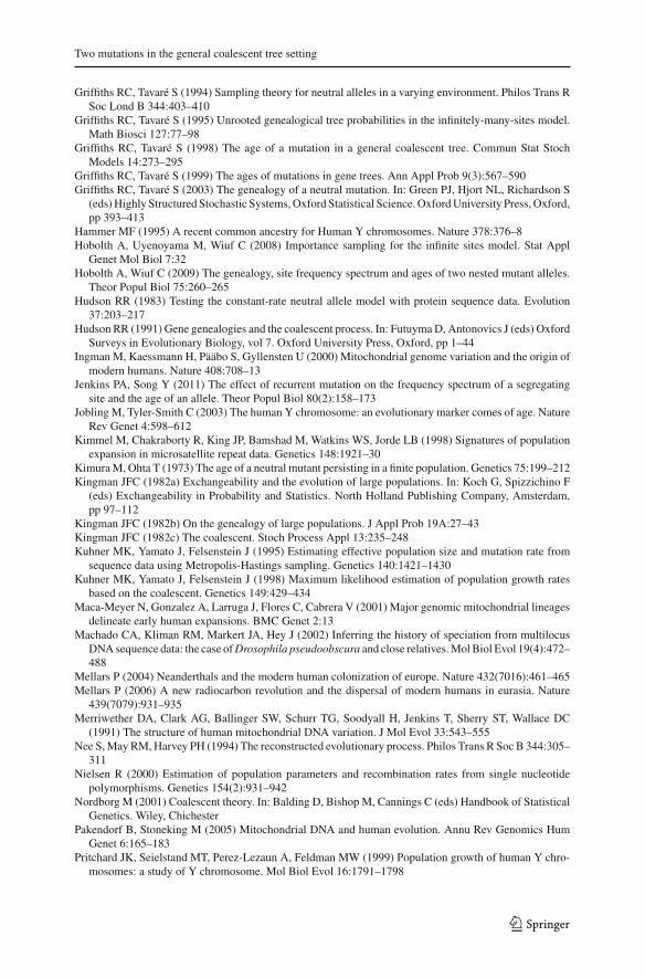
Two mutations in the general coalescent tree setting
Griffiths RC, Tavaré S (1994) Sampling theory for neutral alleles in a varying environment. Philos Trans RSoc Lond B 344:403–410
Griffiths RC, Tavaré S (1995) Unrooted genealogical tree probabilities in the infinitely-many-sites model.Math Biosci 127:77–98
Griffiths RC, Tavaré S (1998) The age of a mutation in a general coalescent tree. Commun Stat StochModels 14:273–295
Griffiths RC, Tavaré S (1999) The ages of mutations in gene trees. Ann Appl Prob 9(3):567–590Griffiths RC, Tavaré S (2003) The genealogy of a neutral mutation. In: Green PJ, Hjort NL, Richardson S
(eds) Highly Structured Stochastic Systems, Oxford Statistical Science. Oxford University Press, Oxford,pp 393–413
Hammer MF (1995) A recent common ancestry for Human Y chromosomes. Nature 378:376–8Hobolth A, Uyenoyama M, Wiuf C (2008) Importance sampling for the infinite sites model. Stat Appl
Genet Mol Biol 7:32Hobolth A, Wiuf C (2009) The genealogy, site frequency spectrum and ages of two nested mutant alleles.
Theor Popul Biol 75:260–265Hudson RR (1983) Testing the constant-rate neutral allele model with protein sequence data. Evolution
37:203–217Hudson RR (1991) Gene genealogies and the coalescent process. In: Futuyma D, Antonovics J (eds) Oxford
Surveys in Evolutionary Biology, vol 7. Oxford University Press, Oxford, pp 1–44Ingman M, Kaessmann H, Pääbo S, Gyllensten U (2000) Mitochondrial genome variation and the origin of
modern humans. Nature 408:708–13Jenkins PA, Song Y (2011) The effect of recurrent mutation on the frequency spectrum of a segregating
site and the age of an allele. Theor Popul Biol 80(2):158–173Jobling M, Tyler-Smith C (2003) The human Y chromosome: an evolutionary marker comes of age. Nature
Rev Genet 4:598–612Kimmel M, Chakraborty R, King JP, Bamshad M, Watkins WS, Jorde LB (1998) Signatures of population
expansion in microsatellite repeat data. Genetics 148:1921–30Kimura M, Ohta T (1973) The age of a neutral mutant persisting in a finite population. Genetics 75:199–212Kingman JFC (1982a) Exchangeability and the evolution of large populations. In: Koch G, Spizzichino F
(eds) Exchangeability in Probability and Statistics. North Holland Publishing Company, Amsterdam,pp 97–112
Kingman JFC (1982b) On the genealogy of large populations. J Appl Prob 19A:27–43Kingman JFC (1982c) The coalescent. Stoch Process Appl 13:235–248Kuhner MK, Yamato J, Felsenstein J (1995) Estimating effective population size and mutation rate from
sequence data using Metropolis-Hastings sampling. Genetics 140:1421–1430Kuhner MK, Yamato J, Felsenstein J (1998) Maximum likelihood estimation of population growth rates
based on the coalescent. Genetics 149:429–434Maca-Meyer N, Gonzalez A, Larruga J, Flores C, Cabrera V (2001) Major genomic mitochondrial lineages
delineate early human expansions. BMC Genet 2:13Machado CA, Kliman RM, Markert JA, Hey J (2002) Inferring the history of speciation from multilocus
DNA sequence data: the case of Drosophila pseudoobscura and close relatives. Mol Biol Evol 19(4):472–488
Mellars P (2004) Neanderthals and the modern human colonization of europe. Nature 432(7016):461–465Mellars P (2006) A new radiocarbon revolution and the dispersal of modern humans in eurasia. Nature
439(7079):931–935Merriwether DA, Clark AG, Ballinger SW, Schurr TG, Soodyall H, Jenkins T, Sherry ST, Wallace DC
(1991) The structure of human mitochondrial DNA variation. J Mol Evol 33:543–555Nee S, May RM, Harvey PH (1994) The reconstructed evolutionary process. Philos Trans R Soc B 344:305–
311Nielsen R (2000) Estimation of population parameters and recombination rates from single nucleotide
polymorphisms. Genetics 154(2):931–942Nordborg M (2001) Coalescent theory. In: Balding D, Bishop M, Cannings C (eds) Handbook of Statistical
Genetics. Wiley, ChichesterPakendorf B, Stoneking M (2005) Mitochondrial DNA and human evolution. Annu Rev Genomics Hum
Genet 6:165–183Pritchard JK, Seielstand MT, Perez-Lezaun A, Feldman MW (1999) Population growth of human Y chro-
mosomes: a study of Y chromosome. Mol Biol Evol 16:1791–1798
123
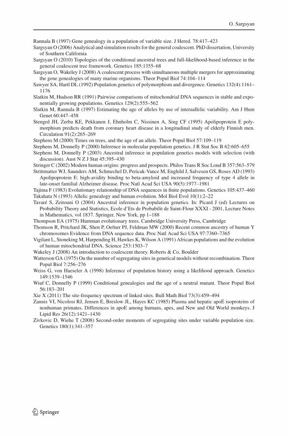
O. Sargsyan
Rannala B (1997) Gene genealogy in a population of variable size. J Hered. 78:417–423Sargsyan O (2006) Analytical and simulation results for the general coalescent. PhD dissertation, University
of Southern CaliforniaSargsyan O (2010) Topologies of the conditional ancestral trees and full-likelihood-based inference in the
general coalescent tree framework. Genetics 185:1355–68Sargsyan O, Wakeley J (2008) A coalescent process with simultaneous multiple mergers for approximating
the gene genealogies of many marine organisms. Theor Popul Biol 74:104–114Sawyer SA, Hartl DL (1992) Population genetics of polymorphism and divergence. Genetics 132(4):1161–
1176Slatkin M, Hudson RR (1991) Pairwise comparisons of mitochondrial DNA sequences in stable and expo-
nentially growing populations. Genetics 129(2):555–562Slatkin M, Rannala B (1997) Estimating the age of alleles by use of interaallelic variability. Am J Hum
Genet 60:447–458Stengrd JH, Zerba KE, Pekkanen J, Ehnholm C, Nissinen A, Sing CF (1995) Apolipoprotein E poly-
morphism predicts death from coronary heart disease in a longitudinal study of elderly Finnish men.Circulation 91(2):265–269
Stephens M (2000) Times on trees, and the age of an allele. Theor Popul Biol 57:109–119Stephens M, Donnelly P (2000) Inference in molecular population genetics. J R Stat Soc B 62:605–655Stephens M, Donnelly P (2003) Ancestral inference in population genetics models with selection (with
discussion). Aust N Z J Stat 45:395–430Stringer C (2002) Modern human origins: progress and prospects. Philos Trans R Soc Lond B 357:563–579Strittmatter WJ, Saunders AM, Schmechel D, Pericak-Vance M, Enghild J, Salvesen GS, Roses AD (1993)
Apolipoprotein E: high-avidity binding to beta-amyloid and increased frequency of type 4 allele inlate-onset familial Alzheimer disease. Proc Natl Acad Sci USA 90(5):1977–1981
Tajima F (1983) Evolutionary relationship of DNA sequences in finite populations. Genetics 105:437–460Takahata N (1993) Allelic genealogy and human evolution. Mol Biol Evol 10(1):2–22Tavaré S, Zeitouni O (2004) Ancestral inference in population genetics. In: Picard J (ed) Lectures on
Probability Theory and Statistics, Ecole d’Ets de Probabilit de Saint-Flour XXXI - 2001, Lecture Notesin Mathematics, vol 1837. Springer, New York, pp 1–188
Thompson EA (1975) Humman evolutionary trees. Cambridge University Press, CambridgeThomson R, Pritchard JK, Shen P, Oefner PJ, Feldman MW (2000) Recent common ancestry of human Y
chromosomes Evidence from DNA sequence data. Proc Natl Acad Sci USA 97:7360–7365Vigilant L, Stoneking M, Harpending H, Hawkes K, Wilson A (1991) African populations and the evolution
of human mitochondrial DNA. Science 253:1503–7Wakeley J (2008) An introduction to coalescent theory. Roberts & Co, BoulderWatterson GA (1975) On the number of segregating sites in genetical models without recombination. Theor
Popul Biol 7:256–276Weiss G, von Haeseler A (1998) Inference of population history using a likelihood approach. Genetics
149:1539–1546Wiuf C, Donnelly P (1999) Conditional genealogies and the age of a neutral mutant. Theor Popul Biol
56:183–201Xie X (2011) The site-frequency spectrum of linked sites. Bull Math Biol 73(3):459–494Zannis VI, Nicolosi RJ, Jensen E, Breslow JL, Hayes KC (1985) Plasma and hepatic apoE isoproteins of
nonhuman primates. Differences in apoE among humans, apes, and New and Old World monkeys. JLipid Res 26(12):1421–1430
Zivkovic D, Wiehe T (2008) Second-order moments of segregating sites under variable population size.Genetics 180(1):341–357
123