Embed Size (px)
Citation preview

AN ANALYSIS OF MULTISPECTRAL UNMANNED AERIAL SYSTEMS
FOR SALT MARSH FORESHORE LAND COVER CLASSIFICATION
AND DIGITAL ELEVATION MODEL GENERATION
by
Logan D. Horrocks
A thesis submitted in fulfillment of the
requirements of GEOG 4526
for the Degree of Bachelor of Science (Honours)
Department of Geography and Environmental Studies
Saint Mary’s University
Halifax, Nova Scotia, Canada
L.D. Horrocks, 2018
April 11th, 2018
Members of the Examining Committee:
Dr. Danika van Proosdij (Supervisor)
Department of Geography and Environmental Studies,
Saint Mary’s University
Dr. Philip Giles
Department of Geography and Environmental Studies
Saint Mary’s University

ii
ABSTRACT
An Analysis of Multispectral Unmanned Aerial Systems for Saltmarsh Foreshore Land
Cover Classification and Digital Elevation Model Generation
by
Logan D. Horrocks
Recent advances in Unmanned Aerial Systems (UAS), and increased affordability, have
proliferated their use in the scientific community. Despite these innovations, UAS attempts to
map a site’s true elevation using Structure from Motion Multi-View Stereo (SFM-MVS) software
are obstructed by vegetative canopies, resulting in the production of a Digital Surface Model
(DSM), rather than the desired Digital Elevation Model (DEM). This project seeks to account for
the varying heights of vegetation communities within the Masstown East saltmarsh, producing
DEMs for mudflat/saltmarsh landscapes with an accuracy comparable to that the DSM. DEM
generation has been completed in two separate stages. The first stage consists of land cover
classifications using UAS derived, radiometrically corrected data. Respective land cover
classifications are assessed using confusion matrices. Secondly, surveyed canopy heights and
function derived heights are subtracted from their respective classes, generating the DEMs. DEM
validation has been performed by comparing topographic survey point values to those modeled,
using the Root Square Mean Error (RMSE) measure. The project then compares the various
parameters implemented for land cover classifications, and DEM accuracy. DEM generation
methods were then coupled to produce a final DEM with a RMSE of 6cm. The results suggest
consumer grade Multispectral UAS can produce DEMs with accuracies comparable to the initial
DSMs generated, and thus merit further studies investigating their scientific capacities.
April 11th, 2018

iii
RÉSUMÉ
Une analyse des systèmes aériens multispectraux téléguidés pour la classification de
la couverture terrestre et la génération numérique de modèles d’élévation dans le cas de
marais estuariens
Par Logan D. Horrocks
Les progrès récents dans les systèmes aériens téléguidés (UAS) et leur accessibilité
croissance ont favorisé leur utilisation au sein de la communauté scientifique. Malgré ces
innovations, les UAS tentent de cartographier l’élévation de la surface d’un site obstrué par la
végétation à partir du logiciel « Motion Multi-View Stereo » (SFM-MVS); aboutissant à la
création d’un Modèle Numérique d’Élévation (MNE) au lieu du Modèle Numérique de Terrain
(MNT) souhaité. Ce projet vise à quantifier les différentes hauteurs des communautés végétales
dans le marais salé de Masstown Est, en produisant des MNE pour les paysages de
marais/vasières avec une précision comparable à celle des MNE. La génération des MNT a été
réalisée à partir de deux étapes distinctes. La première étape repose sur des classifications de la
couverture terrestre à partir de données UAS dérivées, corrigées radiométriquement et
géométriquement. Les classifications de la couverture terrestre sont évaluées à partir de matrices
de confusion. Dans un second temps, les hauteurs de la canopée étudiée et les hauteurs dérivées
de la fonction sont soustraites de leurs classes respectives, générant les MNT. La validation des
MNT a été réalisée en comparant les valeurs des relevés topographiques avec les valeurs
modélisées, en utilisant la mesure de l’erreur quadratique moyenne (EQM). Le projet compare
ensuite les différents paramètres mis en place pour les classifications de la couverture terrestre et
la précision du MNT. Les méthodes de génération de MNT ont ensuite été couplées pour
produire un MNT final avec une EQM de 6 cm. Les résultats indiquent que les UAS
multispectraux « Grand public » peuvent produire des MNT avec des précisions comparables aux
MNE initiaux générés, et mériteraient ainsi d’autres études quant à leur valeur scientifique.
Le 11 Avril, 2018

iv
ACKNOWLEDGEMENTS
This project owes many thanks to many people, without whom this pursuit would not
have been feasible. I would like to thank my supervisor Dr. Danika van Proosdij for her insightful
feedback on a weekly basis which crafted the project to its current state, and my second reader
Dr. Philip Giles for his comprehensive comments and advice.
The completion of this project owes many thanks to Greg Baker for his consultations,
without whom the flights would have been impossible to complete. A big thank-you to Jennie
Graham for her guidance in the vegetation survey, and Graham Matheson for his guidance in the
topographic survey. A big thanks to Sam, Reyhan, and Larissa as well for their help completing
the vegetation surveys, and to Freddie Jacks for all her help with edits.
I owe countless thanks to my Dad and Mom for everything that’s allowed for me to reach
this point. A final thanks to Carl, Dylan, and all my friends for keeping me sane in this period.

v
TABLE OF CONTENTS
Abstract ........................................................................................................................................... ii
Résumé .......................................................................................................................................... iii
Acknowledgements ....................................................................................................................... iv
List of Tables .................................................................................................................................. vi
List of Figures ............................................................................................................................... vii
Chapter 1 Introduction and Literature Review .............................................................................. 1
Chapter 2 Study Area .................................................................................................................. 20
Chapter 3 Methods and Data ....................................................................................................... 23
Chapter 4 Results ........................................................................................................................ 29
Chapter 5 Discussion ................................................................................................................... 48
Chapter 6 Conclusion ................................................................................................................. 57
List of Reference ........................................................................................................................... 59
Appendix ....................................................................................................................................... 66

vi
LIST OF TABLES
Table 1.1: Temporal Resolution Examples via Satellite Return Period ........................................... 6
Table 4.1 Surveyed Monoculture Canopies Mean and Range ....................................................... 30
Table 4.2 Pix4D Project Details ..................................................................................................... 31
Table 4.3: Comparison of DSM, Pix4D and Surveyed Error ......................................................... 33
Table 4.4:Confusion Matrix, 90m, 6 Classes ................................................................................. 40
Table 4.5: Confusion Matrix, 70m, 6 Classes ................................................................................ 41
Table 4.6: Confusion Matrix, 50m, 6 Classes ................................................................................ 41
Table 4.7: Confusion Matrix Using Cell C as Training Data, 90m, 6 classes ............................... 42
Table 4.8: Confusion Matrix Using Cell C as Training Data, 90m, 5 classes ............................... 43
Table 4.9: Confusion Matrix Using Cell AB as Training Data, 90m, 5 classes ............................ 43
Table 4.10: Comparing DEM RMSE per Class ............................................................................. 48

vii
LIST OF FIGURES
Figure 1.1: Spatial Resolution Example ........................................................................................... 4
Figure 1.2: Radiometric Resolution Example. ................................................................................. 5
Figure 1.3: Spectral Resolution Example via Different Sensors. ..................................................... 6
Figure 1.4: Spectral Response Curves.............................................................................................. 8
Figure 1.5: Maximum Likelihood Classifier. ................................................................................. 12
Figure 2.1 (A-C): Study Site, Masstown East Salt Marsh. ............................................................ 21
Figure 2.2: Saltmarsh Zones of Vegetation. Low to High Marsh Transition ................................. 22
Figure 3.1: Site Sample Setup ........................................................................................................ 24
Figure 4.1: Surveyed Canopy Heights Mean ................................................................................. 31
Figure 4.2: DSM Bare Surface Error Per Flight Altitude .............................................................. 32
Figure 4.3: Comparison of DSM Error, 90m RGB and MS .......................................................... 33
Figure 4.4: NDVI and NDRE Maps Generated from 90m MS flight ............................................ 34
Figure 4.5 (A-F): NDVI Canopy Height Functions. ...................................................................... 36
Figure 4.6 (A-F) NDRE Canopy Height Functions. ...................................................................... 37
Figure 4.7: Isocluster Classification, 90M MS .............................................................................. 38
Figure 4.8: Isocluster Classification, 90M MS, Saltmarsh and Borrow Pit ................................... 39
Figure 4.9: Supervised Classification, 6 classes, 90m Multispectral ............................................. 41
Figure 4.10: Class Extents for 50, 70 and 90m Multispectral Supervised Classifications. ........... 44

viii
Figure 4.11:Class Extents for Varying Test Pixel Location, 90m, Supervised Classifications ..... 45
Figure 4.12: Class Masks Derived from the 90m, 6 Class Supervised Classification ................... 46
Figure 4.13: Comparison of DEMs Error at Origin Point Locations ............................................. 47
Figure A.1: S. alterniflora vegetation survey, Cell A .................................................................... 67
Figure A.2: S. alterniflora vegetation survey, Cell C .................................................................... 68
Figure A.3: S. alterniflora vegetation survey, Cell B .................................................................... 69
Figure A.4: S. patens vegetation survey, Cell A ............................................................................ 70
Figure A.5: S. patens vegetation survey, Cell C ............................................................................ 71
Figure A.6: S. patens vegetation survey, Cell B ............................................................................ 72
Figure A.7: G. geradii alive vegetation survey, Cell A ................................................................. 73
Figure A.8: G. geradii alive vegetation survey, Cell C .................................................................. 74
Figure A.9: G. geradii alive vegetation survey, Cell B .................................................................. 75
Figure A.10: G. geradii dead vegetation survey, Cell A ................................................................ 76
Figure A.11: G. geradii dead vegetation survey, Cell C ................................................................ 77
Figure A.12: G. geradii dead vegetation survey, Cell B ................................................................ 78
Figure A.13 (A-F): Cell B S. alterniflora (A-C) and S. patens (D-F) survey images .................... 79
Figure A.14 (A-F): Cell C S. alterniflora (A-C) and S. patens (D-F) survey images .................... 80
Figure A.15 (A-F): Cell B J. geradii alive (A-C) and dead (D-F) survey images ........................ 81
Figure A.16 (A-F): Cell A (A-C) and C (D-F) J. geradii alive survey images ............................ 81
Figure A.17: Pix4D Report for 50 and 70m Multispectral Flights ................................................ 83
Figure A.18: Pix4D Reports for 90m Multispectral and RGB Flights ........................................... 84

1
CHAPTER 1
Introduction and Literature Review
1.1. Introduction
Recent advances and increased affordability in Unmanned Aircraft Systems (UAS)
technology have rendered their use widespread in the scientific community (Colomina and
Molina, 2014; Crutsinger et al., 2016). UAS are comprised of Unmanned Aerial Vehicles
(UAVs), the respective controller system, and the communication system which connects the two
(ICAO, 2011). UAS have been used for numerous applications and disciplines ranging from
agriculture (Horton et al., 2017; Wu et al., 2017), forestry (Hogan et al, 2017), land degradation,
(Yengoh et al., 2015) and conservation (Husson et al., 2017).
The products generated from remote sensing systems are largely limited by vegetation
cover when trying to acquire true landform elevations for Digital Elevation Models (DEMs),
creating Digital Surface Models (DSMs) instead (Carrivick et al, 2016). DEMs of a suitable
accuracy may be used for numerous geomorphic, landform, and hydrographic analyses
(Gonçalves & Henriques, 2015; Jaud et al., 2016). DEMs captured over a successive timespan
may reveal further change within a landscape (Lucieer & Jong, 2014; Haas et al., 2016). Those
who employ remote sensing techniques are faced with the availability of ever-increasing
precision and accuracy of their instruments, coupled with the emergence of new innovations
(Crutsinger et al., 2016). Having examined the tool kits, practices and classifications of others
with larger UAS craft and more refined sensors, it has been suggested that consumer grade
multispectral sensors merit investigation on their capacity to classify saltmarsh covers and

2
produce DEMs (Harwin and Lucieer, 2012; Jaud et al., 2016; Long et al., 2016; Kalacska et al.,
2017). Means of incorporating variables beyond reflectance values (such as elevation) in
multivariate classifications also supported the idea that surface cover delineation could be
successfully performed with a high degree of accuracy (Grebby et al., 2010).
This research will determine what combination of parameters for a multispectral equipped
UAS will yield the most accurate and useful land cover classifications and DEM for the
saltmarsh landscape. These parameters include flight altitudes of 50, 70, and 90 meters,
classification schemes with different five and six landcover classes, and two canopy adjustment
methods for the present species of vegetation. The objective of this project is to produce a DEM
with a tolerable accuracy through generating the suite of geospatial products required. An ideal
accuracy for the DEM would rival the accuracy of the DSM in areas if bare surface (lacking
vegetative cover).
This study employed DJI Phantom 3 Drone modified to carry a Parrot Sequoia
Multispectral Sensor to classify surface covers in the Masstown East Saltmarsh. Following the
classifications of surface covers in the site with kappa coefficients greater than 0.8, the study
seeks to derive DEMs from DSMs for the site by accounting for varying heights of vegetative
communities. The derivation of DEMs with classified covers has been completed with two
separate methods representing canopy height(s). Further analysis exploring supervised
classifications, DEM generation, and their errors has been performed to quantitatively assess the
potential of UAS mounted multispectral sensors. The results from this project may then serve as
guidelines or recommendations regarding project and flight set up for future studies seeking to
employ UAS for scientific research.

3
1.2. Literature Review
This literature review will commence its investigation with an overview of remote
sensing, examining the various impacts of resolution, and the different classification processes.
The development of the Structure from Motion Multi-View Stereo (SfM-MVS) processing and
multispectral sensors for UAS will then be investigated. The review considers the components of
a saltmarsh, followed by investigation of feedbacks within the system using concept of
Ecogeomorphology. Finally, the application of remote sensing systems for mapping saltmarshes
will be examined, illustrating the variety of disciplines that may benefit from the geospatial
products.
1.2.1. Remote Sensing Overview
1.2.1.1. Recent History and Application
In the last twenty years, there have been tremendous developments within the field of
remote sensing of vegetation (Crutsinger, 2016; Aguilera and González, 2017). High resolution
imagery from various sources has reached the most accessible levels in history in terms of price
and availability (Colomina and Molina, 2014), furthering the demand for high quality end
products from a multitude of fields and across various sectors. Among the many uses of remotely
sensed data, the identification and monitoring of land covers and vegetative species remains a key
component for practices such as conservation and restoration (Peacock, 2014; Whitehead and
Hugenholtz, 2015). The ability to produce secondary products such as DSMs and DEMs is also
of high importance for numerous other applications such as the production of slope maps,
average insolation and windspeed maps, used in a variety of other domains (Carrivick et al.,

4
2016). The ability to produce DEMs of a suitable accuracy for further analysis is a function of the
levels of resolution of the sensor and platform in use.
1.2.1.2. Resolution
When acquiring remotely sensed data, there are a few primary considerations which will
guide the entire acquisition process: the purpose of the data, the subject being studied, and the
context. One must have a clear purpose in their pursuit to generate a useful end-product that
properly addresses the fundamental research question. Once addressed, one can start to determine
the resolution needed to observe the desires phenomena. For this to be accomplished, there must
be a solid understanding of the components that make up resolution. Four types of resolution
exist and allow users to determine the suitability of a set of imagery for their selected purpose;
spatial, spectral, radiometric and temporal (Fox III, 2015).
Spatial resolution refers to the size of ground resolution cell (area on the earth),
represented by each pixel in the image. The term ground sample distance (G.S.D) refers to the
distance on earth between the midpoints of pixels. Small objects can be identified in high or fine
spatial resolution (NRCAN, 2013). Following the example in Figure 1.1, there are more pixels
Figure 1.1: Spatial Resolution Example. Reproduced from Giles, P. (2016).
Remote Sensing of the Environment, Class 6: Radiometric Resolution;
Atmospheric influences; Image enhancement.

5
making up a feature in a high spatial resolution image than a low-resolution image (Spring et al.,
2016).
Radiometric resolution refers to the relative widths of brightness intervals. These intervals
can be visualized as the quantity of brightness steps utilized by the image, as shown in Figure 1.2.
A higher radiometric resolution will have more steps than a low-resolution image, thus better
representing the variation in brightness and rendering it more informative (Fox III, 2015). This
can be directly observed in the brightness steps of Figure 1.2.
Spectral resolution describes the wavelength range of spectral bands that make up the
image, with each band denoting a certain range of radiation the sensor is receptive to (Fox III,
2015). An image may be comprised of multiple bands, yet it is only possible to display three at a
time due to the three color guns available (R,G,B) available for display on LCD monitors. Figure
1.3 displays various sets of sensors and their respective spectral resolutions.
Temporal resolution describes the frequency (timespan) between data collections the
sensor and platform are capable of (Fox III, 2015). Depending on the platform in use, the return
time between data collection can vary greatly. Multiple image sets are required to observe,
measure, and compare changes in observed phenomena.
Value Range Number of Brightness Levels Bits
Figure 1.2: Radiometric Resolution Example. Reproduced from: Geographisches
Institut der Universität Bonn. (n.d.). Radiometric Resolution. Retrieved from
http://www.fis.unibonn.de/en/recherchetools/infobox/professionals/resolution/radiomet
ric-resolution

6
Temporal resolution can range anywhere from a 15-minute interval (a drone flight and
replacing batteries), to semi-annually, and potentially even infinitely depending on the platform.
As seen on Table 1.1, there exists a range of temporal resolutions for various satellites. UAS
offer new levels of temporal resolution; the term is increasingly irrelevant for UAS
photogrammetry as flights can be performed as the user desires. A major benefit of UAS is that
the timing and frequency of data collection is under the user’s control. With an understanding of
the four characteristics of resolution and the demands of one’s project, one can start to evaluate
the suitability of different sensors and the host platforms for their desired data (Fox III, 2015).
1.2.1.3. Pre-Processing: Calibrations
As recent advances in the remote sensing industry have led to widespread implementation
and combination of technologies, it becomes increasingly important to objectively evaluate the
products generated. Measures can be taken before and after the flight to achieve the highest
quality of data; these processes are calibration, pre-processing, and post-processing (Kumar,
Figure 1.3: Spectral Resolution Example via Different Sensors. Reproduced
from: Harris Geospatial. (2013). Figure 3: Spectral Resolution of Different
Sensors
Comparison of Sensor’s Spectral Resolution
Table 1.1: Temporal Resolution Examples via
Satellite Return Period. Reproduced from:
Obregon, R. (2009). Table 4: Current and
proposed sensor systems for identifying and
mapping urban features.
Comparison of Sensor’s Temporal Resolution
7
2012). The calibration process takes place before any flights, while both pre-processing and post-
processing occurs after flights. Calibration ensures that the data collected are accurate and
representational of the observed surface. Pre-processing includes rectification, restoration, and
image enhancement, while post-processing concerns itself with information extraction (Kumar,
2012).
Calibration is employed to standardize the results gathered based on the specifics of the
sensor, lens and platform in use. Calibrating a multispectral sensor radiometrically ensures that
the radiance in the images are representative of true surface reflectance (Kumar, 2012), adjusting
for uneven response across the sensor (Crisp, 2001). Targets with standardized reflectance values
can be employed to calibrate the sensor, ensuring it portrays values as intended. Radiometric
calibrations for illumination differences differ greatly for sensors and platforms in use. For
satellites, little can be done in the way of accounting for solar exposure at that given site, while
for UAS, sunlight sensors can be attached atop the platform to account for incoming radiation
(Parrot, 2016). For example, the Parrot Sequoia utilizes a sunlight or ‘irradiance’ sensor to
account for illumination and give absolute measurements (Parrot, 2016).
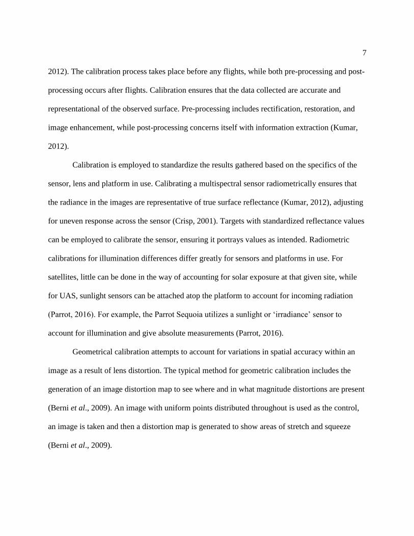
Geometrical calibration attempts to account for variations in spatial accuracy within an
image as a result of lens distortion. The typical method for geometric calibration includes the
generation of an image distortion map to see where and in what magnitude distortions are present
(Berni et al., 2009). An image with uniform points distributed throughout is used as the control,
an image is taken and then a distortion map is generated to show areas of stretch and squeeze
(Berni et al., 2009).
8
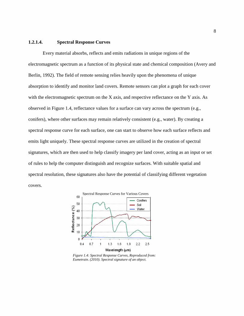
1.2.1.4. Spectral Response Curves
Every material absorbs, reflects and emits radiations in unique regions of the
electromagnetic spectrum as a function of its physical state and chemical composition (Avery and
Berlin, 1992). The field of remote sensing relies heavily upon the phenomena of unique
absorption to identify and monitor land covers. Remote sensors can plot a graph for each cover
with the electromagnetic spectrum on the X axis, and respective reflectance on the Y axis. As
observed in Figure 1.4, reflectance values for a surface can vary across the spectrum (e.g.,
conifers), where other surfaces may remain relatively consistent (e.g., water). By creating a
spectral response curve for each surface, one can start to observe how each surface reflects and
emits light uniquely. These spectral response curves are utilized in the creation of spectral
signatures, which are then used to help classify imagery per land cover, acting as an input or set
of rules to help the computer distinguish and recognize surfaces. With suitable spatial and
spectral resolution, these signatures also have the potential of classifying different vegetation
covers.
Figure 1.4: Spectral Response Curves, Reproduced from:
Eumetrain. (2010). Spectral signature of an object.
Spectral Response Curves for Various Covers
9
There exist many examples where the creation of spectral response curves has been
performed with a high degree of success using high resolution satellite imagery taken with a
hyperspectral sensor (Kokaly 2007, Berni et al., 2008; Grebby et al, 2010; Parent et al., 2015).
There is also a growing trend in UAS based signature generation with the advancements of both
sensor platform and technology (King et al., 2005; Berni et al., 2008; Whitehead and
Hugenholtz, 2015; Heipke 2016; Aguilera and González, 2017). Hyperspectral sensors have
traditionally been the popular choice for species level classifications due to the high spectral
resolution; with narrower and more bands, it is easier to find some region in which the spectral
reflectance properties of species may differ.
1.2.1.5. Post Processing: Unsupervised and Supervised Classification
Post processing involves information extraction processes such as unsupervised and
supervised classification. These processes automate identification of covers quantitatively
(Kumar, 2012). Although some suggest this may replace visual analysis (Kumar, 2012), there
exists limits to the accuracy and reliability of the technology (Crutsinger, 2016).
In remote sensing, image classification is generally grouped into two categories:
unsupervised and supervised classification. Unsupervised Classification “investigates data
statistics by subdividing the image into clusters of pixels with similar characteristics” (Li et al.,
p.1, 2015), most commonly through Iterative Self-Organizing Data Analysis (ISODATA) or K-
mean classification (Li et al., 2015). On the other hand, “Supervised techniques are characterized
by finding explicit relationships between samples and classes” (Li et al., 2015). Unsupervised
classification typically requires less initial time input, but the output is of a different nature than a

10
supervised classification as there is no user defined training datasets (Peacock, 2014). Quality of
the supervised classification is also found to have improved if the user has a previous
understanding of the type of cover in the image (Jensen, 2005).
Signature generation is a process that comes about in the steps of supervised
classification. Supervised classification works with the user specifying pixels that belong to a
certain cover class, (e.g., water). Small polygons are constructed over the raster surface with a
representative range of Digital Number (DN) values within the cover. These are the input training
pixels the computer will use to generate the signatures used for the classification (Rumiser et al.,
2013). Once a representative number of polygons have been constructed to show a representation
of the variation within a class (comprising multiple signatures), a new signature that combines all
is created to be representative of the entire class. For each class and thus each cover, the process
is repeated to make a representative class signature. The class signatures are then saved as a
signature set (Rumiser et al., 2013), and are ready for their first implementation.
The signature set is applied to the image data as the input signature file. Analysis of the
classification can then be performed to determine the number of pixels in each class (Rumiser et
al., 2013), and if any pixels were misclassified in the classification. Following the initial
signature generation, the classification may be repeated with slight modifications to the input
signatures depending on the results. Signatures would be modified by selecting additional
training sites, to include representative pixels omitted (Rumiser et al., 2013). The signature set
and the algorithm are selected to perform the classification. Different algorithms serve as
different guiding rules which will be used to assign all pixel values in the image to a class. This
project has selected the Maximum Likelihood Algorithm.

11
One of the essential steps required in the remote sensing process is ground truthing.
Ground truthing is the selection of ground resolution cells with known cover characteristics as
training sites (NRCAN, 2013). By selecting a plot with known vegetation covers, one can be
certain that the output signatures are as accurate as possible (Rumiser et al., 2013). There is no
set number of training pixels ‘required’ for a supervised classification, however studies often
employ 10n-100n pixels per class, where n is the number of bands input into the classification
(Jensen, 2005). In selecting these pixels, one attempts to select as many sites as required to
represent the entire range of DN values within the cover. Assessments of the sizes and
distribution of plant communities should be considered before any flight as the spatial resolution
of the imagery must be finer than the phenomena that is to be observed.
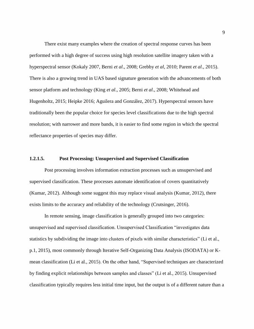
1.2.1.6. Classification Algorithms and Accuracy Assessments
As different algorithms exist to assign unknown pixels to a class, it becomes increasingly
important to understand the logic and the assumptions upon which the algorithms operate. The
algorithm used in this process is the Maximum Likelihood classification. Figure 1.5 graphically
displays how this algorithm operates. Maximum Likelihood assigns unknown pixels to a class by
computing the standard deviations from the multivariate mean for each class and placing pixels in
their most probable class (Kumar, 2012). This algorithm assumes that each class has a normal
distribution in each band. If the data displays a bi-modal or tri-modal distribution, it is likely the
modes should be separate classes (Kumar, 2012). This method of classification is considered to
be the most statistically accurate, and the most computationally demanding (Peacock, 2014).
12
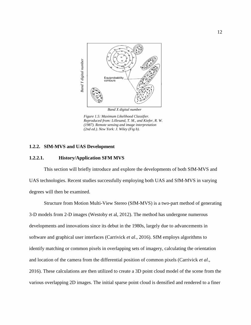
1.2.2. SfM-MVS and UAS Development
1.2.2.1. History/Application SFM MVS
This section will briefly introduce and explore the developments of both SfM-MVS and
UAS technologies. Recent studies successfully employing both UAS and SfM-MVS in varying
degrees will then be examined.
Structure from Motion Multi-View Stereo (SfM-MVS) is a two-part method of generating
3-D models from 2-D images (Westoby et al, 2012). The method has undergone numerous
developments and innovations since its debut in the 1980s, largely due to advancements in
software and graphical user interfaces (Carrivick et al., 2016). SfM employs algorithms to
identify matching or common pixels in overlapping sets of imagery, calculating the orientation
and location of the camera from the differential position of common pixels (Carrivick et al.,
2016). These calculations are then utilized to create a 3D point cloud model of the scene from the
various overlapping 2D images. The initial sparse point cloud is densified and rendered to a finer
Figure 1.5: Maximum Likelihood Classifier.
Reproduced from: Lillesand, T. M., and Kiefer, R. W.
(1987). Remote sensing and image interpretation
(2nd ed.). New York: J. Wiley (Fig b).
Band X digital number
Ba
nd
Y d
igit
al
nu
mb
er

13
resolution, or ‘Dense Point Cloud’ with MVS methods. Carrivick et al. (2016) emphasize that
SFM-MVS methods are still in their infancy, requiring more research and analysis of accuracy to
reach their true potential in the geosciences.
1.2.2.2 Development of UAS Platforms and Respective Sensors
The term UAV has been deemed obsolete by the International Civil Aviation
Organization (2011), yet it is still appearing in much of the academic literature published of late
(Long et al., 2016; Crutsinger et al., 2016). Advancements in sensor and platform technologies
have resulted in the widespread deployment of UASs for multiple purposes, including data
acquisition. As explored by various authors including Colomina and Molina (2014) and Fox III,
(2015), these sensors and platforms are continually becoming less expensive, while delivering
finer and higher resolution data. There has been growing demand for the application and
utilization of UAS technology within the academic community, as more academics learn what
sorts of projects and data acquisition these technologies can perform for them. One of the greatest
advancements this may yield is a shift towards “Remote Sampling” for many disciplines (UK
Marine, 2001). This trend is partially due to the fact UAS technology can acquire high resolution
data without disturbing or negatively impacting the landscape under observation when physically
taking samples from it, or reducing the total area required to physically visit. As the associated
sensor technology increases in terms of both spectral and spatial resolution, so will further
demand for UAS based observation.

14
1.2.2.3. Applied UAS Studies: Multivariate Classifications and Accuracy Assessments
Yengoh et al. (2015) explore the ways in which the NDVI (Normalized Difference
Vegetation Index) can be incorporated in generation of spectral signatures for monitoring land
degradation, agricultural and ecosystem resilience, and desertification. Combined with other
indexes (such as the Normalized Difference Water Index, NDWI), trained analysts can utilize
NDVI further monitor drought, land productivity, carbon stocks, and habitat fragmentation
(Yengoh et al, 2015; Stow et al, 2007). Other have sought higher spatial and spectral resolution
data for precision application, such as Viticulture. Satesteban (2016) incorporated thermal
imagery retrieved from a UAS to generate a crop water stress index (CWSI) representative of the
site. Signatures can also be created using additional variables if they are in the exact same raster
format; this process is called multivariate classification (Roe, 2006). Integrating the multispectral
rasters with both NDVI and elevation data can yield a more accurate classification (Sturari et al.,
2017). A study done by Grebby et al., (2010), attempted this, and generated lithological maps
using the relationship between plants and topography. They found upon incorporating elevation
data that they were about to improve their kappa coefficient from 65.5 to 88%. Furthermore,
thermal imagery and the Normalized Difference indexes it can generate can be incorporated into
the multivariate classification for an even more detailed product (Berni et al., 2008). Although
additional variable inputs for a multivariate classification can produce more accurate and detailed
products, there remains sets of assumptions and limits for every product.

15
1.2.3. Saltmarsh Landscape, Form and Ecogeomorphology
1.2.3.1. Macrotidal creek form and zonation of vegetation
This section will provide a review of the components that make up the dynamic system of
the saltmarsh landscape and their interactions. Fagherazzi et al. (2002) describe the saltmarsh as a
system in which the feedback between biota and landscape is extremely strong. They state that
this relationship is strong enough to play a role in how these landscapes evolve, as well as their
fate (Fagherazzi et al., 2002).
Thus, to understand the landscape and its morphology requires an understanding of the
biota, and vice versa. The Masstown Saltmarsh may be described as a finger marsh; a long marsh
existing along a tidal channel (UMaine, 2017). Saltmarsh landscapes have been categorized by
Amos (1995) into three main zones: the subtidal zone, the intertidal zone and the supratidal zone.
As their names suggest, the subtidal zone occurs below the low water mark, while the supratidal
zone occurs above the high tide mark. The intertidal zone is located between the other two, the
high and low marks water respectively (Amos, 1995). The intertidal zone can be divided into
three main zones: Tidal Flat/ Channel, Low Marsh and High Marsh (UMaine, 2017). Within the
intertidal zone there exist a common zonation of vegetation. As noted by Fagherazzi et al. (2004),
the zonation of vegetation species within the saltmarsh is a function of hydroperiod and salinity,
and thus elevation and distance from tidal creeks also plays a role in determining what species
will grow in a given location. For the case of the majority of salt marshes within the Minas basin,
the low marsh is dominated by Spartina alterniflora; a marsh grass that thrives in the saline
conditions and diurnal inundation (Allen, 2000). The high marsh is host to a larger diversity of

16
species with various salt tolerances but is generally dominated by Spartina patens and Juncus
geradii (UMaine, 2017).
1.2.3.2. Ecogeomorphology: the Saltmarsh Landscape
The dynamic nature of the saltmarsh giving rise to its form and function is better
understood through the concept of Ecogeomorphology. The discipline is defined as “the study of
the coupled evolution of geomorphological and ecosystem structures” Fagherazzi, (2004, p. vii).
As a dynamic system, a saltmarsh with the proper conditions can keep pace with sea level
rise (Throne et al., 2013). This process requires adequate accretion, either by minerogenic,
surface deposition, or organogenic, subsurface accumulation (Allen, 1990), or a combination of
the two. Saltmarsh vegetation such as Spartina alterniflora and Spartina patens exert a source of
friction on the flowing tide, reducing flow velocity and wave action (Lightbody and Nepf, 2006).
Pending an adequate reduction in velocity, the suspended particles in the water column can settle
on the marsh surface (Lightbody and Nepf, 2006). The same vegetative covers account for
subsurface accretion, through an accumulation of organic matter as rhizomatic root mats undergo
their life cycles (Allen, 1990). Vegetative covers contribute to the composition of the marsh;
Rinaldo et al., (2004) found interactions between the patterns in vegetation and the morphology
of the marsh surface are key components of the landscape’s dynamics. As tidal platforms accrete
to elevation levels conducive of colonization by halophytic species (e.g., Spartina alterniflora),
the network reaches a form of dynamic equilibrium and experiences only minor alterations
afterwards (Rinaldo et al., 2004.)

17
1.2.4. Application of Remote Sensing in Saltmarshes
1.2.4.1. Application of UAS and Remote Sensing in Saltmarshes
This section will investigate the various projects within saltmarsh ecosystems that have
employed UAS technology. These projects can be divided into two broad classes: orthomosaics
and elevation models. As reviewed in previous sections, SFM -MVS and UAS technologies have
undergone significant advancements in the past five years (Crutsinger, 2016; Aguilera and
González, 2017; Carrivick et al., 2016). This has allowed some to claim that SFM-MVS will
'revolutionize' analysis of tidal systems (Kalacska et al., 2017). Numerous projects utilizing UAS
and SFM-MVS have reported elevation error values ranging from 1.5cm - 10cm (Harwin and
Lucieer, 2012; Jaud et al., 2016; Long et al., 2016; Kalacska et al., 2017) within saltmarsh
landscapes, with sensors ranging from Red, Green Blue (RGB); Multispectral; and Light
Detection and Ranging (LIDAR) capabilities.
When comparing the DSMs of saltmarshes derived from LiDAR and SFM-MVS to DGPS
surveyed elevations, Kalacska et al. (2017) found UAS average elevation error in the range of
2.1-3.6 cm, and 13-29 cm for LiDAR respectively. They claim LiDAR coverage, although
quicker that SFM-MVS and DGPS surveys and less intrusive, does not provide the required
resolutions required to analyze features of interest (Kalacska et al., 2017).
Notably, Medeiros et al. (2015) and Hladik and Alber (2012) attempted to produce valid
DEMs representative of the tidal flats elevation by accounting for the varying heights and
biomass of vegetation species. Medeiros et al., (2015) employed a methodology that examined
the relation between biomass measurements to remotely sensed data for each class and created
species independent LiDAR DSM adjustment values to more accurately determine tidal platform
18
elevation. RMSE of the LiDAR derived DEM was improved from 0.65m to 0.40m when
incorporating the adjustment values (Medeiros et al., 2015).
Recent development in the field of remote sensing describes the new possibilities
emerging for both researchers and practitioners (Colomina and Molina, 2014). Remote sensing
researchers are faced with an ever-increasing precision and accuracy of their instruments, coupled
with the emergence of new ones (Crutsinger et al., 2016). The examination of the tool kits and
practices of others suggest that multispectral imagery is effective for generation of monoculture
specific spectral signatures and image classification. Means of incorporating variables beyond
multispectral imagery (such as elevation) in a multivariate classification also supports the idea
that species identification can be successfully performed (Grebby et al., 2010). Further research
attempting supervised classification, comparing outputs and their errors, needs to be performed to
quantitatively asses the suitability and accuracy of UAS mounted multispectral sensors for
vegetation species identification.
1.2.4.2. The Anthropogenic and Ecological Importance of Saltmarshes
As complex and diverse ecosystems, saltmarshes provide food and habitat to a vast range
of species. Saltmarshes provide humans with countless benefits, quantified as ecosystem services
(Biodiversity Information System for Europe, 2010). These services range in their nature and
output, yet many aspects of our culture and economy are dependent upon them (JCU, 1995;
Sousa et al., 2016). Their ecological importance and our dependence on these systems has led
many to call for their conservation and continued monitoring (Chmura, 2013; Hopkinson et al.,
2012; Deegan et al., 2012; Beaumont et al., 2013).

19
Saltmarshes have been found to be tremendous sequesters of carbon (Macreadie 2014;
Beaumont et al., 2013). The plant communities within the marsh, largely Spartina alterniflora
and Spartina patens, perform photosynthesis and convert C02 in the atmosphere into sugars,
which are stored in their root masses. As these undergo cycles of thriving and perishing, carbon is
accumulated below ground (Allen, 1990). It is estimated that saltmarshes sequester 4.6 – 8.7
teragrams of carbon dioxide annually (Quintana-Alcantara and Eduardo, 2014). The system is
important for other nutrient cycles, including that of nitrogen and potassium (Sousa et al., 2010).
The saltmarsh is also the habitat of many vegetative, invertebrate, fish, and bird species (Wiegert
et al., 1981). Atlantic Canadian saltmarshes are home to rare and endangered species including
the piping plover (Environment Canada, 2012) and Eastern Lilaeopsis and Eastern Baccharis
(GOC, 2017).
The saltmarsh provides a valuable coastal barrier for any feature immediately upland of
the marsh (Pendle, 2013). Not only does the saltmarsh thrive on regular tidal inundations, but the
vegetation within the marsh dissipates oncoming wave energy (Lightbody and Nepf, 2006).
Moreover, saltmarshes are increasingly valuable when they are in front of a dyke feature, as they
can greatly reduce maintenance costs associated with waves and storms (Gedan et al., 2011;
Pendle, 2013).

20
CHAPTER 2
Study Area: Masstown East
2.1. Masstown East Overview
The area of study is the eastern portion of the Masstown Saltmarsh, located in the Minas
Basin, Nova Scotia. The Minas Basin is in the upper reach of the Bay of Fundy as seen in Figure
2.1. It is a macrotidal system, possessing a tidal range of 16m at its peak (NOAA, 2017). The site
has high concentrations of suspended sediment, with maximums in the range of 6 g/l (G.
Matheson, personal communication, August 2017). The marsh is minerogenic, with organic
matter contents ranging from 0.5% - 4 % respectively (Matheson, personal communication,
August 2017). The site has experienced a historic trend of progradation (Matheson, personal
communication, March 2018), as well as having been dyked and being historically managed this
way (Landscape of Grand Pre, 2017). Within the marsh, the practice of digging borrow pits has
been employed to provide material to top the dykes, keeping the agricultural land behind the
structure from flooding. This practice requires excavating channels in the marsh, or ‘pits’ as a
source of material for dyke topping (Bleakney, 2004). The borrow pits within the Masstown East
saltmarsh have demonstrated trends of infill of 10-15 cm/year over the past year (Matheson,
personal communication, March 2018), and being colonized by the low marsh species Spartina
alterniflora. The borrow pit and dyke features result in cross sectional elevation profiles that are
atypical relative to non-modified marsh platforms.
21
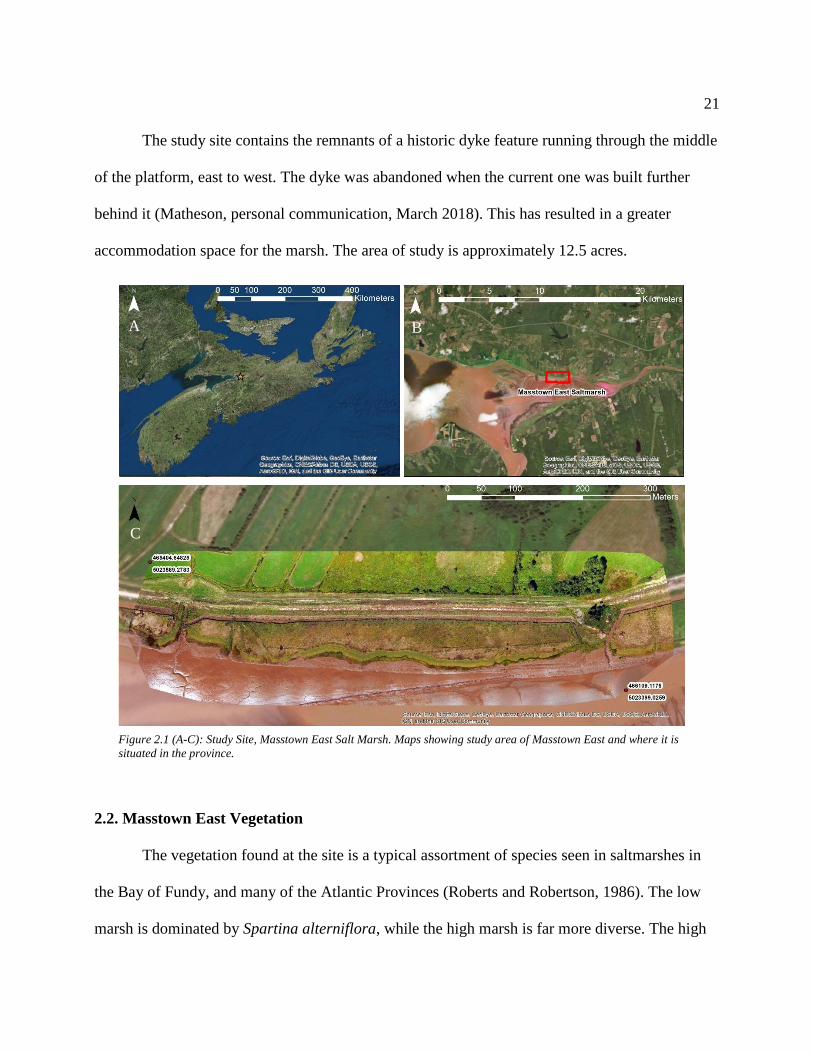
The study site contains the remnants of a historic dyke feature running through the middle
of the platform, east to west. The dyke was abandoned when the current one was built further
behind it (Matheson, personal communication, March 2018). This has resulted in a greater
accommodation space for the marsh. The area of study is approximately 12.5 acres.
2.2. Masstown East Vegetation
The vegetation found at the site is a typical assortment of species seen in saltmarshes in
the Bay of Fundy, and many of the Atlantic Provinces (Roberts and Robertson, 1986). The low
marsh is dominated by Spartina alterniflora, while the high marsh is far more diverse. The high
Figure 2.1 (A-C): Study Site, Masstown East Salt Marsh. Maps showing study area of Masstown East and where it is
situated in the province.
A B
C

22
marsh at the site is covered predominately in Spartina patens and Juncus Geradii. Other species
within this zone include Solidago sempervirens (Seaside goldenrod), Limonium vulgare (Seaside
Lavender), Triglochin maritima (Arrowgrass), Glaux maritima (Sea Milkwart), and Spartina
pectinata.
The distribution and assortment of vegetation is visibly distinguishable in RGB imagery,
appearing as bands parallel to the thalweg and running East-West in the site. The first band
adjacent to the channel is the Spartina alterniflora monoculture, while the next higher band
above it is largely Spartina patens with some Spartina alterniflora and Trilochin maritima. The
last and uppermost zone is the High Marsh mix, largely consisting of patched of healthy and dead
Juncus geradii, and small mixes of the mentioned high marsh species.
Figure 2.2: Saltmarsh zones of vegetation. Low to high marsh
transition, low marsh in foreground, high marsh in background.
Reproduced from: Zottoli, R. (2015, April 14). Spartina patens (Zone
3).
Saltmarsh
Vegetation
Zonation High Marsh
Low Marsh

23
CHAPTER 3
Methodology and Data
3.0. Project Methodology
While the field of UAS remote sensing and SFM-MVS are still in their infancy, there
lacks the extensive body of research on methods and accuracy that exists for satellite platforms.
This project couples both methodologies previously tested in UAS applications with those
inspired by methods used for other platforms and sensors. Methods and sequences in this project
have been adopted from previous work and the respective findings, when possible. For example,
G.C.P. orientation and deployment has been optimized from previous Maritime Provinces Spatial
Analysis Research Center (Mp_Sparc) UAS flights and their outputs. The remaining sequences
(such as orientation and deployment of training/testing polygons) were informed by the academic
body of knowledge on the specific subject (e.g. training pixels for UAS derived data), and the
broader subject (e.g. training pixels for data derived from all platforms) where additional
information is required. The rigor of the sample set up was constrained by the time and funds
available for the project and seeks to maximize product accuracy. The project consists of three
core aspects: field work and ground truthing, Pix4D processing, and ArcGIS processing.
3.1. Field Work and Ground Truthing
A segment of the marsh spanning an area feasible to cover by foot was selected for the
study site, spanning about 600m by 50- 90m. The segment of marsh was then divided into three
cells labeled A, B and C, about 200m each in length as shown in Figure 3.1. The sample set of

24
one training polygon (2x2m) for each vegetated cover in each cell was then configured. The
potential locations for polygons were determined using freely available satellite imagery of the
site on Google Earth. Points with these locations for each polygon were then input into a Garmin
handheld GPS unit for the field (+/- 5m).
Vegetation survey quadrats of 0.5m by 0.5m were constructed and strung. Each quadrat
was divided into a 5x5 square grid, with 25 squares measuring 10x10cm each. This area
corresponds roughly to the G.S.D. of the Parrot Sequoia when flown at an altitude of 90m.
Polygon measuring ropes to deploy training polygons were crafted using 8m segments of
nylon rope with the ends tied together. The rope was marked at a one-meter interval with flagging
Figure 3.1: Site Sample Setup

25
tap to allow square and rapid deployment of the polygon. In the field, dowels were used to deploy
the polygon. Following the vegetation survey, the dowels were replaced with flags for the
topographic survey. The rope was then removed and used to guide the next training polygon.
This method ensured all polygons were of a comparable area and geometry.
The vegetation surveys were performed three times in each polygon to validate the
certainty of cover in the area. The locations of the vegetation survey with the polygon were
chosen by a Random Number Generator (RNG) between 1-16. Each polygon of 2x2m can be
divided into a grid of 4x4 with 16 cells measuring 0.5m by 0.5m each. These configurations were
chosen as vegetation surveys require a minimum of 15% of an area to be surveyed to quantify
covers within (USGS/NPS, 1994). As each of the three quadrats was 0.25 m2, roughly 19% of
each 4m2 training polygon was sampled. Tables and images from the vegetation survey are
included in the appendix
The orientation of G.C.P.s attempts to minimize the number of G.C.P.s deployed, while
spacing them appropriately through the study site. A minimum spacing of G.C.P.s is calculated as
1.5 times the smallest image dimension (Mpsparc, 2017). This calculated spacing ensures there is
an adequate number of G.C.P.s visible in each image. As this project flew at various altitudes, the
lowest altitude image dimensions were used for the G.C.P. spacing calculation. G.S.D. is the term
used by the Pix4D program to describe the GRC of a given project. The G.S.D. of the UAS at
50m was 6.2cm, while the smallest dimension of image is 960 pixels. The product of the G.S.D.
and pixels was multiplied by 1.5 to suggest a spacing of 90m.Therefore, G.C.P.s were not spaced
more than 90m from the edge of the study site, or each other. This ensures that there is minimal
warping and distortion within the DSM of the study site.
26
G.C.P.s were deployed on September 14th, and the UAS flights completed between the
14th and the 15th. The flights were completed with a 85% frontlap and a 70% sidelap between
images, nadir, and at altitudes of 50, 70, and 90m respectively. All G.C.P.S, polygon vertices,
and vegetation survey locations were surveyed using the Leica GS-14 GNSS RTK Rover, with
sub-centimeter horizontal and vertical accuracies.
Vegetation surveys included a list of species, hits (where species intersects with the
survey grid), percent cover, plant height (height of the entire plant), and canopy height (the height
at which the plant stands). Canopy height and plant height may be identical or may vary greatly if
the plant ‘lays’ on the ground. An image was taken with a GPS camera at the location of each
survey. The images include the plot, the quadrat, and a labeled whiteboard detailing the survey
number. Percent cover was estimated based on visual observation, while all other measurements
were collected quantitatively. Canopy heights were measured with a metal rod that had an
adjustable and locking perpendicular piece (the arm). The rod was planted vertically in the
ground and the arm locked at a height estimated to be representative of the mean canopy height.
The rod was gently rotated, and the arm adjusted to intersect the maximum amount of canopy
tops within its radius. The arm’s final height above the surface is the mean canopy height for the
area.
3.2. Pix4D Processing
The images collected from the various flights were uploaded into Pix4D mapping
software, where initial point clouds are generated. The point clouds are then georeferenced with
DGPS coordinates for each G.C.P. visible in the imagery set. The projected error for these

27
coordinates are also input into this process. For multispectral imagery sets, images taken prior to
each flight of an Airnov calibration target (with known reflectance values) were used to
radiometrically correct the Sequoia image and sunshine sensors. The processing parameters for
the project are then set and run, generating the dense point cloud. From this point cloud, the
DSM, orthomosaics and reflectance maps were generated and exported.
3.3. ArcGIS Processing
The data was amalgamated into an ArcGIS database. All data were input in the NAD 83
CSRS Zone 20N horizontal coordinate system and the CGVD 2013 vertical datum. Once all
reflectance maps were input, indices were generated. For this project, an NDVI raster was
generated from the NIR and Red reflectance maps at the varying altitudes. The project also
generated and utilized the Normalized Difference Red Edge (NDRE) index (Spiral Commercial
Services, 2015; MicaSense, 2017), using the NIR and Red Edge reflectance maps.
Following the generation of the indices, polygon and vegetation survey points were
plotted. Polygons were created for each class by joining the surveyed vertices. Within these
polygons, several iterations of random points were generated, with spacing corresponding to the
G.S.D. Approximately 200 training and testing points were generated within each of the
polygons. An intersection was then performed and all testing pixels within 13.3cm of a training
pixel were deleted, ensuring no training or testing pixels exist in the same location and reducing
the count below 200. The points served to break up the surveyed region into fragments, one set of
shapefiles for testing pixels, and one set for training pixels. Shapefiles of training and testing
pixels were also created using the pixels for each cover within Cells A and B, and Cell C.
28
Supervised classifications of the different flights were then completed with the randomly
generated training pixels within sets of shapefiles, within the surveyed locations. Classifications
were run using six classes for all three altitudes with all data available in the scene.
Classifications were run using the 90m multispectral dataset using seven, six and five classes to
represent to covers within the imagery. These classifications employed the Maximum Likelihood
algorithm. Each classification then underwent an accuracy assessment with a confusion matrix to
compare the error within each classification (Jensen, 2005). The various confusion matrices were
then compared to consider error amongst different altitudes and training sample selections. Once
a classification scheme with a minimum error and an extent that captured the entire area of study
was selected, DEMs generation began.
DEMs were generated by isolating the vegetation classes as shapefiles and applying
canopy adjustments to respective classes on the DSM. Two methods were employed to determine
canopy adjustment values: a flat subtraction method, and a function-based method. The flat
subtraction method was produced using mean canopy height of the class at the time of the first
vegetation survey. The second method utilized functions portraying relationships between
reflection indices and canopy height for a given pixel.
Canopy height was determined by subtracting RTK elevation values from the UAS
derived canopy elevation values, at the polygon vertices. These heights were then plotted against
remotely sensed variables (e.g., NDVI, NDRE) to examine any relationships that may exist
between the two, and their strength. Adjustment functions were generated from the data that
exhibited continually increasing function and a strong (>0.7) R value. The raster exhibiting the
correlation was then clipped with the respective class shapefile or ‘mask’, and then transformed

29
with the respective function, generating a raster of canopy adjustment values. The raster
generated for each class was subtracted from the DSM, generating the DEM.
The results for the adjustments were then compared to elevation values of the origin
points from the vegetation survey. RMSE was then calculated for the adjustments and compared
between DEM generation methods. RMSE was calculated for both DEMs with the following
equation:
𝑅𝑆𝑀𝐸 = √∑ (𝑃 − 𝑂)2𝑛
𝑖=1
𝑛
P is the predicted value, and O the observed value. The DEM generation methods were then
coupled, utilizing the best of each method to produce a DEM with the maximum accuracy. The
RMSE values for the surveyed bare surfaces was then added to the running error count,
producing a final RMSE value for the DEM.
30
CHAPTER 4
Results
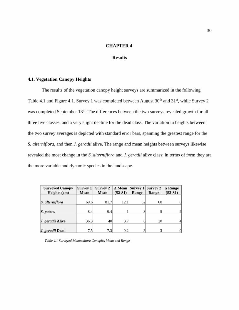
4.1. Vegetation Canopy Heights
The results of the vegetation canopy height surveys are summarized in the following
Table 4.1 and Figure 4.1. Survey 1 was completed between August 30th and 31st, while Survey 2
was completed September 13th. The differences between the two surveys revealed growth for all
three live classes, and a very slight decline for the dead class. The variation in heights between
the two survey averages is depicted with standard error bars, spanning the greatest range for the
S. alterniflora, and then J. geradii alive. The range and mean heights between surveys likewise
revealed the most change in the S. alterniflora and J. geradii alive class; in terms of form they are
the more variable and dynamic species in the landscape.
Surveyed Canopy
Heights (cm)
Survey 1
Mean
Survey 2
Mean
Δ Mean
(S2-S1)
Survey 1
Range
Survey 2
Range
Δ Range
(S2-S1)
S. alterniflora 69.6 81.7 12.1 52 60 8
S. patens 8.4 9.4 1 3 5 2
J. geradii Alive 36.3 40 3.7 6 10 4
J. geradii Dead 7.5 7.3 -0.2 3 3 0
Table 4.1 Surveyed Monoculture Canopies Mean and Range

31
4.2. Pix4D Products
The reports automatically generated from Pix4D gives a variety of information on the
structure for motion process which constructs the reflectance maps and DSMs. The following
table summarizes the Pix4D projects, allowing for comparison amongst the different datasets. All
projects report a relatively low RMSE value for DSM elevation, from 1.6 and 2.6 cm. As the
lower flights were unable to capture the entire marsh surface, the number of G.C.P.s and the area
covered in those datasets are lower. The file size for the projects ranges 15gb for the 90m RGB to
4.5gb for the 70m multispectral (MS). While the 90m RGB and MS flights cover nearly the same
area, the file size for the 90m MS project is roughly two thirds the size of its RGB counterpart.
Project 50m MS 70m MS 90m MS 90m RGB
G.S.D. (cm) 5.26 7.22 9.41 3.84
Extent (ha) 7.36 9.41 19.25 20.29
Number of G.C.P.s 8 7 13 13
RMSE (cm) 1.6 2.2 1.7 2.6
Project File Size (GB) 5.55 4.57 10.2 15 Table 4.2 Pix4D Project Details
0
20
40
60
80
100
Survey 1 Survey 2
Can
op
y H
eight
(cm
)Surveyed Canopy Height Means
S. alterniflora S. patens J. geradii Alive J. geradii Dead
Figure 4.1: Surveyed Canopy Heights Mean
32
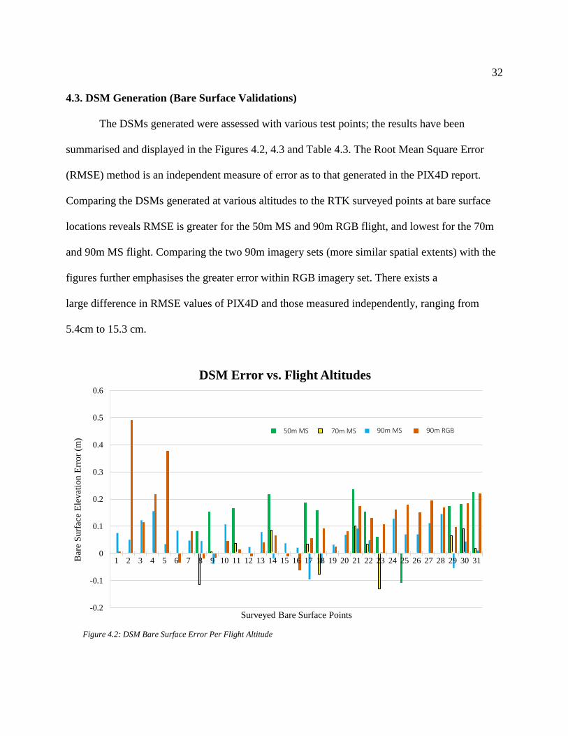
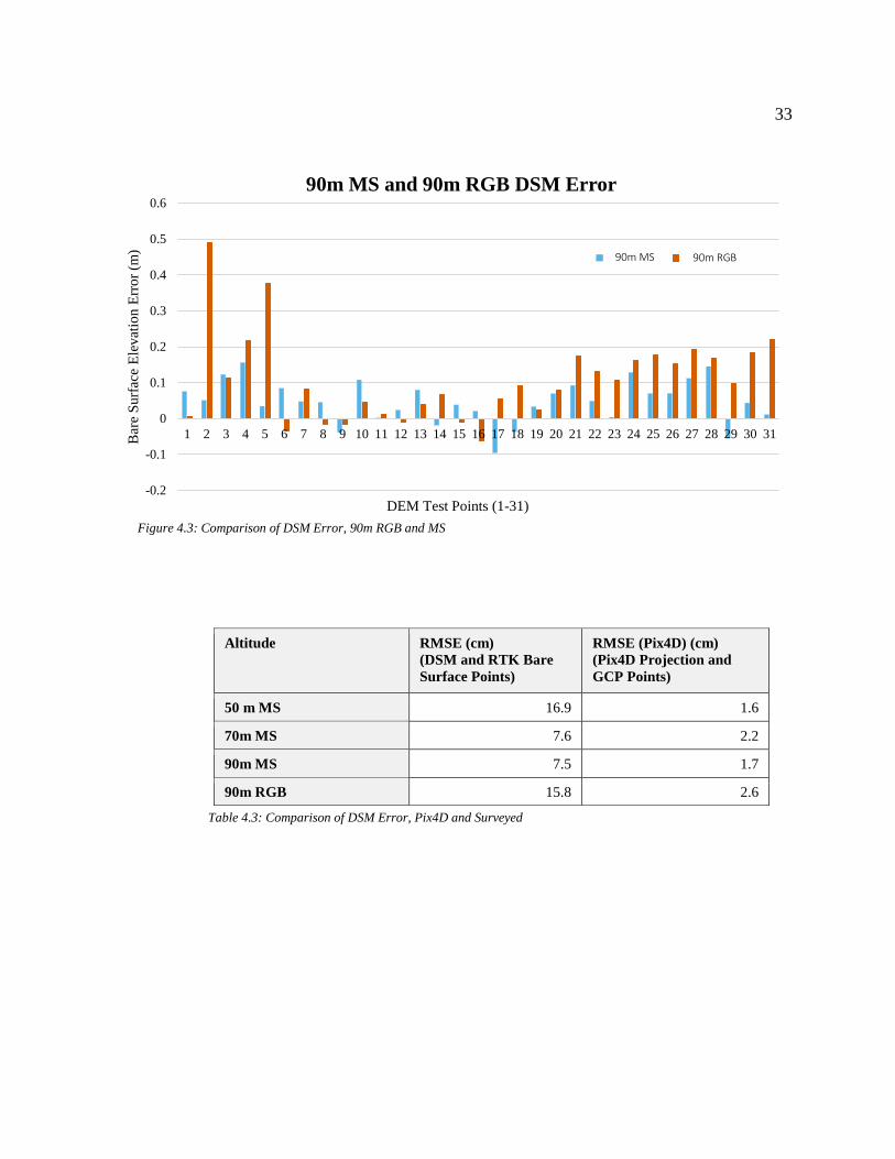
4.3. DSM Generation (Bare Surface Validations)
The DSMs generated were assessed with various test points; the results have been
summarised and displayed in the Figures 4.2, 4.3 and Table 4.3. The Root Mean Square Error
(RMSE) method is an independent measure of error as to that generated in the PIX4D report.
Comparing the DSMs generated at various altitudes to the RTK surveyed points at bare surface
locations reveals RMSE is greater for the 50m MS and 90m RGB flight, and lowest for the 70m
and 90m MS flight. Comparing the two 90m imagery sets (more similar spatial extents) with the
figures further emphasises the greater error within RGB imagery set. There exists a
large difference in RMSE values of PIX4D and those measured independently, ranging from
5.4cm to 15.3 cm.
Altitude RMSE (cm) RSM (Pix4D) (cm) ΔRMSE
(Survey –Pix4D)
(cm)
50 m MS 16.9 1.6 15.3
70m MS 7.6 2.2 5.4
90m MS 7.5 1.7 5.8
90m RGB 15.8 2.6 13.2
-0.2
-0.1
0
0.1
0.2
0.3
0.4
0.5
0.6
1 2 3 4 5 6 7 8 9 10 11 12 13 14 15 16 17 18 19 20 21 22 23 24 25 26 27 28 29 30 31Bar
e S
urf
ace
Ele
vat
ion E
rro
r (m
)
Surveyed Bare Surface Points
DSM Error vs. Flight Altitudes
∆ 50m ∆ 70m ∆ 90m ∆ 90m rgb
Figure 4.2: DSM Bare Surface Error Per Flight Altitude
90m MS 90m RGB 70m MS 50m MS
33
Altitude RMSE (cm)
(DSM and RTK Bare
Surface Points)
RMSE (Pix4D) (cm)
(Pix4D Projection and
GCP Points)
50 m MS 16.9 1.6
70m MS 7.6 2.2
90m MS 7.5 1.7
90m RGB 15.8 2.6
Table 4.3: Comparison of DSM Error, Pix4D and Surveyed
Figure 4.3: Comparison of DSM Error, 90m RGB and MS
-0.2
-0.1
0
0.1
0.2
0.3
0.4
0.5
0.6
1 2 3 4 5 6 7 8 9 10 11 12 13 14 15 16 17 18 19 20 21 22 23 24 25 26 27 28 29 30 31Bar
e S
urf
ace
Ele
vat
ion E
rro
r (m
)
DEM Test Points (1-31)
90m MS and 90m RGB DSM Error
∆ 90m ∆ 90m rgb90m RGB 90m MS

34
4.4. Indices:
Analysis of the NDVI map, Figure 4.4, reveals three distinct regions from foreshore to
pasture. The foreshore mud has extremely low NDVI values, appearing dark. The saltmarsh has a
low to mid-range of NDVI values and is less bright than the pasture and farmland with the
highest NDVI values. There are some very low NDVI values visible as dark patches occurring in
the middle of the saltmarsh platform. The NDRE map lacks the contrast the NDVI map provides
between saltmarsh and pasture.
Figure 4.4: NDVI and NDRE Maps generated from 90m MS flight
Index
Legends

35
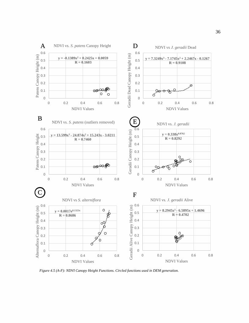
4.5. Canopy Heights vs. Index Values
The following section summarizes the process in which the relationships for the function-
based DEM subtraction were determined. Figures 4.5 (A-F) and 4.6 (A-F) display normalized
differential index values on the X axis, and Canopy height (DSM Elevation - RTK elevation) on
the Y axis. The trendlines describe a relationship between the variables, while the R values are
used to asses the strength of the relationship. Comparison of DSM/RTK derived canopy heights
and index relationships reveals a variety of both weak and moderately strong R values.
The figures with a circled letter (Figure 4.5 C&E, Figure 4.6 B) display the functions with
moderate R values and a trend of consistent increase (no instance of decrease in canopy height
throughout the function); these are the functions utilized for DEM creation. Figure 4.5 E was
generated using data from both J. geradii classes to obtain a function that that expresses both
stages of the species lifecycle. The R value in Figure 4.5 E is higher than all other functions
created in attempt to portray a consistently increasing relationship between J. geradii and a
reflectance index. Rendering the axis of Figure 4.6 B to the same scale as the rest of the figures
makes it hard to observe the binomial trendline; resembling a parabola approaching its vertex.
The removal of two outliers in Figure 4.6 A to create 4.6 B raised the R value from 0.26 to 0.76.
Most attempts to represent the relationship between canopy heights and reflectance index
values yielded functions with low R values as seen in the Figures included in the appendix. Some
attempts returned high R values, yet possessed fluctuating trendlines, such as Figure 4.5 D and
4.6 E.
36
y = -0.1389x2 + 0.2425x + 0.0059
R = 0.1603
0
0.1
0.2
0.3
0.4
0.5
0.6
0 0.2 0.4 0.6 0.8
Pat
ens
Can
op
y H
eight
(m)
NDVI Values
NDVI vs. S. patens Canopy Height
y = 13.599x3 - 24.874x2 + 15.243x - 3.0211
R = 0.7460
0
0.1
0.2
0.3
0.4
0.5
0.6
0 0.2 0.4 0.6 0.8
Pat
ens
Can
op
y H
eight
NDVI Values
NDVI vs. S. patens (outliers removed)
y = 0.0017e8.1323x
R = 0.8686
0
0.1
0.2
0.3
0.4
0.5
0.6
0 0.2 0.4 0.6 0.8Alt
ernaf
lora
Can
op
y H
eight
(m)
NDVI Values
NDVI vs S. alterniflora
y = 7.3249x3 - 7.1745x2 + 2.2467x - 0.1267
R = 0.9108
0
0.1
0.2
0.3
0.4
0.5
0.6
0 0.2 0.4 0.6 0.8
Ger
adii
Dea
d C
ano
py H
eight
(m)
NDVI Values
NDVI vs J. geradii Dead
y = 0.338x0.8762
R = 0.8292
0
0.1
0.2
0.3
0.4
0.5
0.6
0 0.2 0.4 0.6 0.8
Ger
adii
Can
op
y H
eight
(m)
NDVI Values
NDVI vs. J. geradii
y = 8.2945x2 - 6.5895x + 1.4696
R = 0.4702
0
0.1
0.2
0.3
0.4
0.5
0.6
0 0.2 0.4 0.6 0.8
Ger
adii
Ali
ve
Can
op
y H
eight
(m)
NDVI Values
NDVI vs. J. geradii Alive
Figure 4.5 (A-F): NDVI Canopy Height Functions. Circled functions used in DEM generation.
A
B
C
D
E
F

37
y = -485.11x3 + 218.29x2 - 31.639x +
1.5812
R = 0.5119
0
0.1
0.2
0.3
0.4
0.5
0.6
0 0.05 0.1 0.15 0.2
Pat
ens
Can
op
y H
eiht
(m)
NDRE Values
NDRE vs S. patens
y = -12.065x2 + 4.3375x - 0.2604
R = 0.8761
0
0.1
0.2
0.3
0.4
0.5
0.6
0 0.05 0.1 0.15 0.2
Pan
tens
Can
op
y H
eight
(m)
NDRE Values
NDRE vs S. patens (outliers removed)
y = 3.173x - 0.136
R = 0.5143
0
0.1
0.2
0.3
0.4
0.5
0.6
0 0.05 0.1 0.15 0.2
Alt
ernaf
lora
Can
op
y H
eight
(m)
NDRE Values
NDRE vs. S. alterniflora
y = 25.038x2 - 8.1733x + 0.8274
R = 0.3434
0
0.1
0.2
0.3
0.4
0.5
0.6
0 0.05 0.1 0.15 0.2
Ger
adii
Ali
ve
Can
op
y H
eight
(m)
NDRE Values
NDRE vs. J. geradii Alive
y = 1.6987x1.2751
R = 0.6383
0
0.1
0.2
0.3
0.4
0.5
0.6
0 0.05 0.1 0.15 0.2
Ger
adii
Can
op
y H
eight
(m)
NDRE Values
NDRE vs. J. geradii
y = 228.09x2 - 51.235x + 2.9305
R = 0.9186
0
0.1
0.2
0.3
0.4
0.5
0.6
0 0.05 0.1 0.15 0.2
Ger
adii
Dea
d C
ano
py H
eight
(m)
NDRE Values
NDRE vs. J. geradii Dead
Figure 4.6 (A-F) NDRE Canopy Height Functions. Circled function used in DEM generation.
A
B
C
D
E
F

38
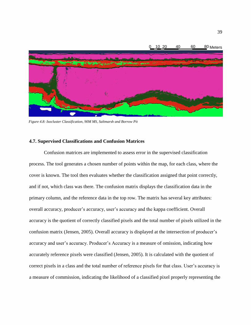
4.6. Isocluster Classification
Isocluster classifications with various parameters were completed on the 90m MS dataset
to make some initial observations about the data and its potential. The following Figures 4.7 and
4.8 are the results of an eight class Isocluster classification using the 90m MS DSM, reflectance
maps, NDVI and NDRE as input rasters.
This initial classification managed to separate several key features out of the dataset,
while classifying several unique features into the same class. For example, class 4 contains the S.
alterniflora patches, borrow pits and a large section of pasture in the upper right of the map.
Class 6 contains the high marsh community on the marsh platform and some patches of shrub and
tree community in the upper half of the map. To further examine the classification, a black
delineation of the foreshore from 2017 was applied over the map. As seen on Figure 4.7, the
divide between classes 3 and 4 seems to portray the foreshore/saltmarsh edge. Shown in Figure
4.8, the divide between classes 4 and 5 seems to correspond to the saltmarsh/burrow pit edge, and
the S. alterniflora and S. patens zones.
Figure 4.7: Isocluster Classification, 90M MS
0 20 4010 Mete Foreshore 2017 1 2
3 4
5 6
7 8
¯
Isocluster Classification Legend
39
4.7. Supervised Classifications and Confusion Matrices
Confusion matrices are implemented to assess error in the supervised classification
process. The tool generates a chosen number of points within the map, for each class, where the
cover is known. The tool then evaluates whether the classification assigned that point correctly,
and if not, which class was there. The confusion matrix displays the classification data in the
primary column, and the reference data in the top row. The matrix has several key attributes:
overall accuracy, producer’s accuracy, user’s accuracy and the kappa coefficient. Overall
accuracy is the quotient of correctly classified pixels and the total number of pixels utilized in the
confusion matrix (Jensen, 2005). Overall accuracy is displayed at the intersection of producer’s
accuracy and user’s accuracy. Producer’s Accuracy is a measure of omission, indicating how
accurately reference pixels were classified (Jensen, 2005). It is calculated with the quotient of
correct pixels in a class and the total number of reference pixels for that class. User’s accuracy is
a measure of commission, indicating the likelihood of a classified pixel properly representing the
0 20 40 60 80 10 Meters
Figure 4.8: Isocluster Classification, 90M MS, Saltmarsh and Borrow Pit

40
land cover (Story and Congalton, 1986; Jensen, 2005). It is calculated with the quotient of correct
pixels in a class and the total number of pixels assigned into the class (Jensen, 2005). The kappa
coefficient is indicative of the agreement between the reference data and the classification map
(Congalton, 1991, Jensen 2005). In its generation, both chance agreement and the overall
accuracy are taken into account (Rosenfield and Fitzpatrick-Lins, 1986; Congalton, 1991; Jensen,
2005). The tables are in part summarized by the kappa coefficient, a measure of how well the
classification map fits the surveyed data. The number of test points was set to 1600 for each class
in the following matrices comparing different flight altitudes but varied based on what was
captured within the respective flight.
4.7.1 Supervised Classifications and Confusion Matrices: Varying Flight Altitudes
As shown in the three confusion matrices, there is very little difference in the kappa
coefficient amongst the three flight altitudes. All classifications possess very high kappa
coefficients ranging from 0.98 to 1. Amongst these classifications, user and Producer’s Accuracy
errors occur mainly in the J. geradii classes. Table 4.4 displays the multispectral 90m, six class
classification utilized in DEM creation.
Class Value Alterniflora Patens
Geradii
Alive
Geradii
Dead Mud BP Total
User’s
Accuracy Kappa
Alterniflora 1600 0 0 0 0 0 1600 1
Patens 6 1594 0 0 0 0 1600 0.9962
Geradii
Alive 0 0 1498 102 0 0 1600 0.9363
Geradii
Dead 0 0 0 1600 0 0 1600 1
Mud 0 0 0 0 1600 0 1600 1
Borrow Pit 0 0 0 0 0 1600 1600 1
Total 1606 1594 1498 1702 1600 1600 9600 0
Producer’s
Accuracy 0.9962 1 1 0.94 1 1 0 0.9887
Kappa 0.9865
Table 4.4:Confusion Matrix, 90m MS, 6 Classes

41
Class Value Alterniflora Patens
Geradii
Alive
Geradii
Dead Mud BP Total
User’s
Accuracy Kappa
Alterniflora 740 0 0 0 0 0 740 1
Patens 0 1099 0 0 0 0 1099 1
Geradii
Alive 0 0 1034 0 0 0 1034 1
Geradii
Dead 0 0 0 758 0 0 758 1
Mud 0 0 0 0 1118 0 1118 1
Borrow Pit 0 0 0 0 0 841 841 1
Total 740 1099 1034 758 1118 841 5590 0
Producer’s
Accuracy 1 1 1 1 1 1 0 1
Kappa 1
Table 4.5: Confusion Matrix, 70m MS, 6 Classes
Class Value Alterniflora Patens
Geradii
Alive
Geradii
Dead Mud BP Total
User’s
Accuracy Kappa
Alterniflora 740 0 0 0 0 0 740 1
Patens 0 590 0 0 0 0 590 1
Geradii
Alive 0 0 550 15 0 0 565 0.973
Geradii
Dead 0 0 0 758 0 0 758 1
Mud 0 0 0 0 1118 0 1118 1
Borrow Pit 0 0 0 0 0 841 841 1
Total 740 590 550 773 1118 841 4612 0
Producer’s
Accuracy 1 1 1 0.981 1 1 0 0.996
Kappa 0.996
Table 4.6: Confusion Matrix, 50m MS, 6 Classes
Figure 4.9: Supervised Classification, 6 classes, 90m multispectral
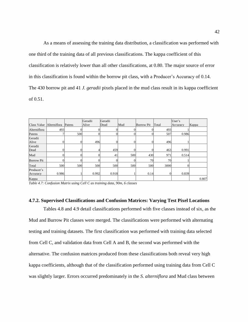
42
As a means of assessing the training data distribution, a classification was performed with
one third of the training data of all previous classifications. The kappa coefficient of this
classification is relatively lower than all other classifications, at 0.80. The major source of error
in this classification is found within the borrow pit class, with a Producer’s Accuracy of 0.14.
The 430 borrow pit and 41 J. geradii pixels placed in the mud class result in its kappa coefficient
of 0.51.
Class Value Alterniflora Patens
Geradii
Alive
Geradii
Dead Mud Borrow Pit Total
User’s
Accuracy Kappa
Alterniflora 493 0 0 0 0 0 493 1
Patens 7 500 0 0 0 0 507 0.986
Geradii
Alive 0 0 496 0 0 0 496 1
Geradii Dead 0 0 4 459 0 0 463 0.991
Mud 0 0 0 41 500 430 971 0.514
Borrow Pit 0 0 0 0 0 70 70 1
Total 500 500 500 500 500 500 3000 0
Producer’s Accuracy 0.986 1 0.992 0.918 1 0.14 0 0.839
Kappa 0.807
Table 4.7: Confusion Matrix using Cell C as training data, 90m, 6 classes
4.7.2. Supervised Classifications and Confusion Matrices: Varying Test Pixel Locations
Tables 4.8 and 4.9 detail classifications performed with five classes instead of six, as the
Mud and Burrow Pit classes were merged. The classifications were performed with alternating
testing and training datasets. The first classification was performed with training data selected
from Cell C, and validation data from Cell A and B, the second was performed with the
alternative. The confusion matrices produced from these classifications both reveal very high
kappa coefficients, although that of the classification performed using training data from Cell C
was slightly larger. Errors occurred predominately in the S. alterniflora and Mud class between
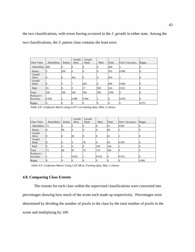
43
the two classifications, with errors having occurred in the J. geradii in either state. Among the
two classifications, the S. patens class contains the least error.
Class Value Alterniflora Patens
Geradii
Alive
Geradii
Dead Mud Total User’s Accuracy Kappa
Alterniflora 469 0 0 0 0 469 1 0
Patens 5 500 0 0 0 505 0.990 0
Geradii Alive 0 0 493 0 0 493 1 0
Geradii
Dead 0 0 7 483 0 490 0.986 0
Mud 26 0 0 17 500 543 0.921 0
Total 500 500 500 500 500 2500 0 0
Producer’s Accuracy 0.938 1 0.986 0.966 1 0 0.978 0
Kappa 0 0 0 0 0 0 0 0.972
4.8. Comparing Class Extents
The extents for each class within the supervised classifications were converted into
percentages showing how much of the scene each made up respectively. Percentages were
determined by dividing the number of pixels in the class by the total number of pixels in the
scene and multiplying by 100.
Table 4.8: Confusion Matrix using Cell C as training data, 90m, 5 classes
Class Value Alterniflora Patens Geradii Alive
Geradii Dead Mud Total User’s Accuracy Kappa
Alterniflora 73 0 0 0 8 81 0.901 0
Patens 0 86 0 0 0 86 1 0
Geradii Alive 0 0 82 0 0 82 1 0
Geradii
Dead 0 0 5 78 0 83 0.939 0
Mud 0 0 0 0 168 168 1 0
Total 73 86 87 78 176 500 0 0
Producer’s Accuracy 1 1 0.942 1 0.954 0 0.974 0
Kappa 0 0 0 0 0 0 0 0.966
Table 4.9: Confusion Matrix Using Cell AB as Training data, 90m, 5 classes
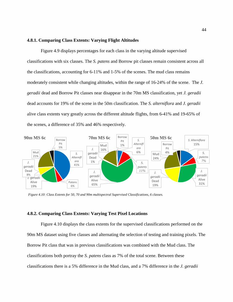
44
4.8.1. Comparing Class Extents: Varying Flight Altitudes
Figure 4.9 displays percentages for each class in the varying altitude supervised
classifications with six classes. The S. patens and Borrow pit classes remain consistent across all
the classifications, accounting for 6-11% and 1-5% of the scenes. The mud class remains
moderately consistent while changing altitudes, within the range of 16-24% of the scene. The J.
geradii dead and Borrow Pit classes near disappear in the 70m MS classification, yet J. geradii
dead accounts for 19% of the scene in the 50m classification. The S. alterniflora and J. geradii
alive class extents vary greatly across the different altitude flights, from 6-41% and 19-65% of
the scenes, a difference of 35% and 46% respectively.
4.8.2. Comparing Class Extents: Varying Test Pixel Locations
Figure 4.10 displays the class extents for the supervised classifications performed on the
90m MS dataset using five classes and alternating the selection of testing and training pixels. The
Borrow Pit class that was in previous classifications was combined with the Mud class. The
classifications both portray the S. patens class as 7% of the total scene. Between these
classifications there is a 5% difference in the Mud class, and a 7% difference in the J. geradii
S. Alternifl
ora
6%
S.
patens
11%J. geradiiAlive 65%
J. geradiiDead1%
Mud16%
Borrow
Pit
1%
70m MS 6c
S. Alternifl
ora41%
Patens6%
J. geradiiAlive 19%
J. geradiiDead
8%
Mud21%
Borrow Pit5%
90m MS 6cS. Alterniflora
15%
S.
patens
7%
J. geradiiAlive 31%
J. geradiiDead19%
Mud24%
Borrow
Pit
4%
50m MS 6c
Figure 4.10: Class Extents for 50, 70 and 90m multispectral Supervised Classifications, 6 classes.

45
Dead class. There is a greater difference in the extents of the S. alterniflora and J. geradii alive
classes between classifications, 13% and 15% respectively.
4.9. DEM Generation
4.9.1 Class Masks
Having performed the classifications and comparing the accuracies amongst them, the
90m flight shows the greatest extent with a minimal sacrifice of accuracy. The 90m dataset has
thus been selected for use in DEM creation. Figure 4.11 is a display of the class-shapes extracted
from the 90m MS, six class classification. These class shapes or ‘masks’ were used for to subtract
the canopy heights, thereby generating a DEM.
Figure 4.11:Class Extents for Varying Test Pixel Location, 90m multispectral Supervised
Classifications, 5 classes.
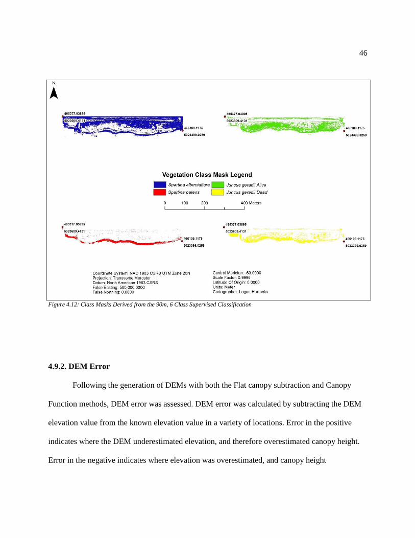
46
Figure 4.12: Class Masks Derived from the 90m, 6 Class Supervised Classification
4.9.2. DEM Error
Following the generation of DEMs with both the Flat canopy subtraction and Canopy
Function methods, DEM error was assessed. DEM error was calculated by subtracting the DEM
elevation value from the known elevation value in a variety of locations. Error in the positive
indicates where the DEM underestimated elevation, and therefore overestimated canopy height.
Error in the negative indicates where elevation was overestimated, and canopy height
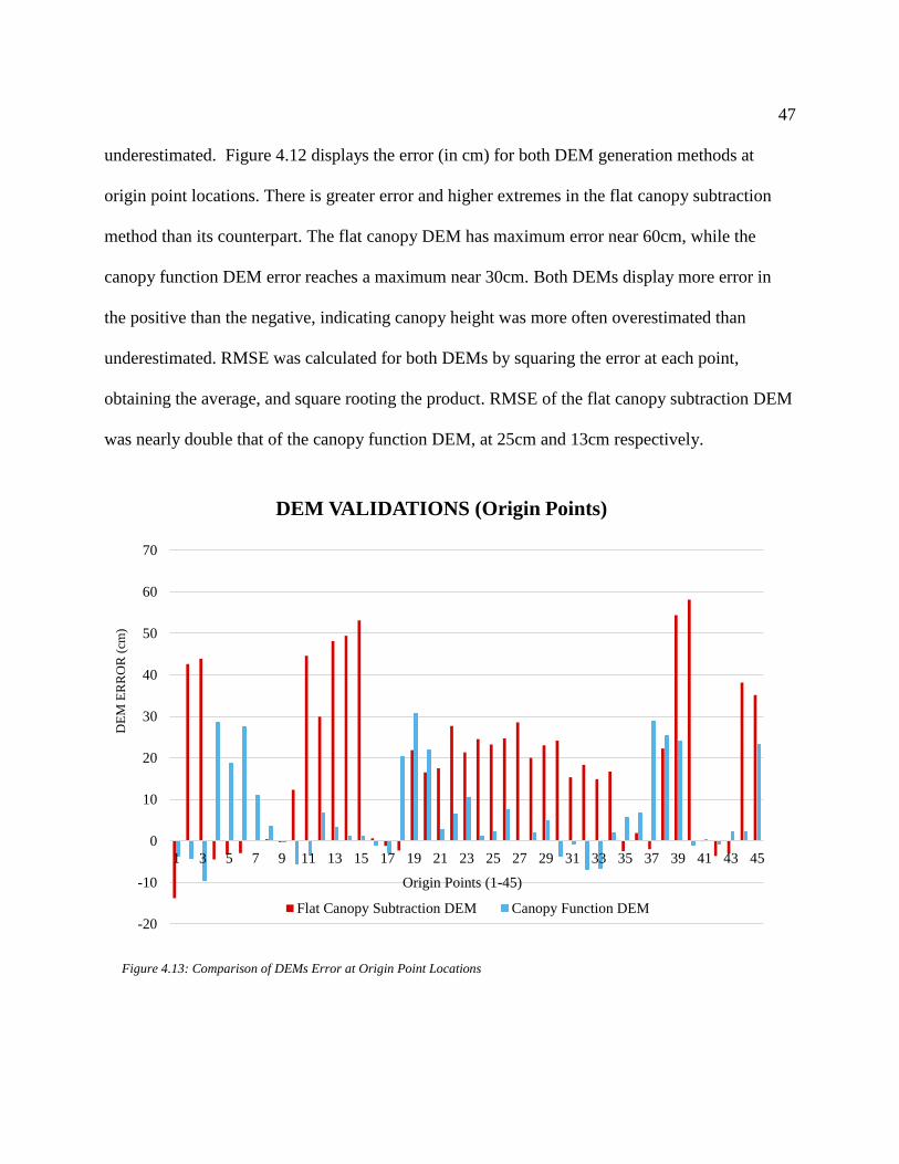
47
underestimated. Figure 4.12 displays the error (in cm) for both DEM generation methods at
origin point locations. There is greater error and higher extremes in the flat canopy subtraction
method than its counterpart. The flat canopy DEM has maximum error near 60cm, while the
canopy function DEM error reaches a maximum near 30cm. Both DEMs display more error in
the positive than the negative, indicating canopy height was more often overestimated than
underestimated. RMSE was calculated for both DEMs by squaring the error at each point,
obtaining the average, and square rooting the product. RMSE of the flat canopy subtraction DEM
was nearly double that of the canopy function DEM, at 25cm and 13cm respectively.
-20
-10
0
10
20
30
40
50
60
70
1 3 5 7 9 11 13 15 17 19 21 23 25 27 29 31 33 35 37 39 41 43 45
DE
M E
RR
OR
(cm
)
Origin Points (1-45)
DEM VALIDATIONS (Origin Points)
Flat Canopy Subtraction DEM Canopy Function DEM
Figure 4.13: Comparison of DEMs Error at Origin Point Locations

48
4.9.3. Calculating RMSE per Class
RMSE was calculated for within the DEMs for each of the landcover classes to compare how
accurately each method represented individual classes. Table 4.10 displays the RMSE within
each class for both DEMs, and total RMSE at the bottom. The second column displays RMSE for
the flat subtraction DEM calculated with Origin points, while the third is calculated with Vertex
points. The fourth column displays RMSE per class for the function method DEM. The flat
subtraction method most accurately portrays the S. patens class, while the other three vegetation
classes are best represented with the function method. The fifth and sixth column represent ‘Post
Results’ of the project. The fifth column represents a DEM crafted with the S. patens class of the
first method, and all other classes using the second. The total RMSE for the resulting ‘coupled’
DEM is 6cm, roughly half that of the function method DEM. The sixth and final column adds the
RMSE of the bare surfaces to the DEM to further assess the surface portrayal. RMSE does not
significantly change with the addition of the Bare surface validation points, retaining a value of
6cm.
Results Post Results
RMSE PER CLASS
(cm)
Flat
Subtraction
DEM (Origin
points)
Flat Subtraction
DEM (Vertex
points)
Function
Subtraction
DEM (Origin
points)
Flat and Function
Subtraction DEM
(Origin and
Vertex points)
Flat and Function
Subtraction DEM
(Origin, Vertex
and Bare Surface)
S. alterniflora 35 44 9 9 9
S. patens 5 4 24 4 4
J. geradii Alive 20 16 3 3 3
J. geradii Dead 1 5 3 3 3
Bare Surface RMSE NA NA NA NA 7
RMSE TOTAL (cm) 26 25 13 6 6
Table 4.10: Comparing DEM RMSE per Class

49
CHAPTER 5
Discussion
5.1. Project Review
This research sought to determine what combination of parameters for a multispectral
equipped UAS would yield the most accurate and useful land cover classifications and DEMs for
the saltmarsh landscape. This section sequentially investigates the various components of the
project and their role in the achievement of the final goal. In the generation of the suite of
geospatial products, error compounds, and must be reduced at each step along the way (Jensen,
2005; Carrivick et al., 2016). The individual aspects of the project have been discussed in terms
of their successes, the assumptions they rely on, and the limitations they are constrained by.
Suggestions for improvements, future directions and considerations have been included for each
of these aspects. This project was able to produce a final DEM with an RMSE comparable to that
of its source DSM, 6cm.
5.2. Field Work and Ground Truthing
The vegetation surveys were completed in two sets, the first on August 30th and 31st, and
the second on September 13th. The vegetation and topographic surveys would both have benefited
from a more rigorous sample set up. Effort would have been better spent capturing more
training/testing data than completing formal vegetation surveys. For this type of ground truthing,
a simple validation of homogenous cover, DGPS survey and image would suffice. The formal

50
survey can take upwards of a half hour if multiple species were present. Those surveys were not
used because of the significant diversity at those locations and the impact of mixed pixels on the
classification (Jensen, 2005). This type of project may also benefit from a combination of formal
and informal validations. A few formal validations would be performed followed by many
informal validations, all surveyed with DGPS. In this case, species could be surveyed on the fly
as one discovers it in a site. The canopy sampling method is somewhat subjective when trying to
determine the mean canopy height for sparser and tall growing vegetation.
The vegetation showed greater variability within the S. alterniflora and J. geradii Alive.
These classes had a greater range and change in canopy height between the surveys than S. patens
and J. geradii Dead classes. These findings compare to other studies examining the species
(Smith et al., 1980; Mӧller, 2006). The growth for all live classes and decline in height for the
dead class between surveys confirm their described states.
Drone flights were completed with varying degrees of difficulty. The 90m RGB flight
was easy to accomplish, the UAS working as it was supposed to. The flights with the Parrot
Sequoia sensor were far less user friendly and required several test flights for trouble shooting
purposes. The issue remained an inability to completely load a mission grid, resulting in the craft
hovering in a fixed location and wasting battery. As a result, all the multispectral flights were
flown manually. The 90m MS flight was completed quickly with two batteries. The 50 and 70m
MS flights would have taken more time than was available to cover the entire marsh surface, thus
50 and 70m were only flown for half the site. These lower altitude flights cover less area, capture
fewer G.C.P.s while requiring them to be closer together (MP_SpARC, 2017), but deliver a
smaller G.S.D.. Radiometric calibration is less accurate for longer flights as more time elapses
51
between the calibration image and last image in the flight set; meanwhile illumination conditions
change. Considering the feasibility, time, and resources, the slight improvements in G.S.D. do not
merit flying at lower altitudes in the saltmarsh landscape.
5.2. Pix4D: DSM Production and Limitations
The SFM-MVS processing supplied via the Pix4D software was user friendly and easy to
follow. The outputs were generated relatively fast; each project was processed within a night. The
subscription fee for the Pix4D software is expensive but facilitates much of the SFM-MVS
processing, requiring the user to set the project parameters and georectify. The software is a bit
of a black-box with some algorithms and processes not fully disclosed. This is not surprising
given the developing nature of SFM-MVS software (Carrivick et al., 2016). Considering the
Pix4D reports, the 90m MS delivered best ratio of coverage to file size, but at the sacrifice of
G.S.D.
The RMSE reported from Pix4D was inconsistent with independently measured RMSE
values. Reported RMSE values ranged 5-15 cm less than the independently measured bare
surface points. Validation points on the edge of the 70 and 50m DSMs were removed as the
significantly higher values were due to the impact of the bowl like warp that exists on the edge of
the DSM (MP_SpARC, 2017). Removing these outliers brought down the RMSE of the 50 and
70m flight from 30 and 40cm to their current 15 and 7cm. There was more error in the 90m RGB
than 90m MS which came across a slightly surprising. The difference in error may be a product
of the georectification process. In the 90m RGB dataset, the center of G.C.P. flag may appear as
1,2,4 or 9 pixels. In the 90m MS dataset it usually shows up as 1 or 4 pixels, making it much

52
easier for the user to remain consistent throughout the process (Jensen, 2005). Error was most
similar between the 90m RGB and 50m MS set, and between the 70 and 90m MS sets. This may
suggest that reducing flight altitude (thereby reducing G.S.D) may be related to increased error.
5.3. Generation of Indices and Canopy Height Statistics
A brief visual analysis of the indices shows the NDVI has more contrast amongst
features, while the NDRE appears very grey and somewhat noisy. There seems to be some
brightness banding in the NDRE which may be an artifact and sunlight reflecting off the wet mud
surface. NDRE is supposed to reveal crop health in late season (Spiral Commercial Services,
2015; MicaSense, 2017), yet there is not nearly as much variation in the marsh platform in NDRE
as in NDVI. This is especially true for the center high marsh region where J. geradii is found
both dead and alive. NDVI portrays the contrast between dead and alive J. geradii, suggesting
perhaps NDRE is not as effective in observing saltmarsh phenology as the maturation of crops.
The creation of functions for the DEM adjustment values operates under the assumption
supported by Medeiros et al., (2015); as canopy height (and thus biomass) increases, so should
reflectance, or brightness in the respective index. An ideal function would reach an asymptote as
the maximum canopy height was reached and would possess a high R value (greater than 0.7),
indicating a strong effect size (Moore et al., 2013). Simpler functions were sought, giving
preference to linear and exponential functions over polynomial ones.
The DEM creation could have benefited from the use of more points for determining
relationships; more vegetation survey points with elevation values would allow for this. These

53
functions should employ 20-30 points per class, greater than the minimum population sample size
(10 points per class) required for regression analysis (Statistics Solutions, 2018).
Strong R values were observed for some trends, but trends fluctuated as NDVI and
NDRE increased. It was deemed fluctuations contradicted the assumption the relationships
operated upon and are thus not used (Medeiros et al., 2015). In hindsight, fluctuations may have
been the result of training site locations where the vegetation is blown over or laying down rather
than upright (accounting for low canopy heights), thus exposing more of the plants surface to the
sky above (accounting for higher index values). Outliers were removed from the S. patens class
as the canopy height values did not correspond to those measured manually. It proved difficult to
observe a strong relationship between the two variables for the S. patens class. J. geradii alive
and dead proved difficult to derive functions for that didn’t fluctuate or have a low R value. J.
geradii classes were then combined as they are the same species, producing an ideal trend line
with a strong R value.
5.4. Land Cover Classifications, Confusion Matrices and Class Extents
The Isocluster classification proved effective for delineating the marsh/foreshore
boundary as seen with the 2017 foreshore line. The classification incorrectly classifies some
features, for example the vegetation in Figure 4.7 between the dyke road and ditch is classified
the same as the high marsh region. The low marsh region is portrayed with lime green, red and
dark green. In Figure 4.8, the red area in front of the marsh corresponds roughly to the S.
alterniflora zone, and the dark green to the S. patens. The pasture behind the dyke is largely
represented with the red and dark green classes. This may reflect the influence of the DSM on the

54
classification (Roe, 2016). Overall, the Isocluster classification displays promise for further
accurately classifying the data
It is recognized that the sample set up was not as extensive as it could have been and
speaks to the balance of a robust sample set up, and what is physically possible. Classification
kappa coefficients reflect a sample set up that could have been more robust with their very high
values. Attempts were taken to assess the sample set up by varying and using portions of the
training and testing data. In all supervised classifications produced, there is salt and pepper effect.
The notion that one of the classifications scored a kappa coefficient of 1 sparks the
interest to re-perform the classifications with a more robust training sample set up, as this result
seems unobtainable (Jensen, 2005). All confusion matrices seem to demonstrate very high kappa
coefficients, suggesting classifications accurately performed at the test point locations. The
changes in altitude do not seem to have an impact in classification accuracy. These high kappa
coefficients are likely a reflection of the training and testing pixel locations (Jensen, 2005).
The next method used to assess the capacity of the training data was alternating test pixel
locations. The classification run using six class and training data only from Cell C reveals a
kappa coefficient of 0.8, a relatively successful classification (Jensen, 2005). The successes of the
classification suggest that there is validity to the training sample set up, as a relatively successful
map can be performed with one third of the input data.
High kappa coefficients were observed for the 90m 5 class classifications which
employed alternating training and testing data. One classification utilized Cell AB and training
data and cell C as validation, while the other utilized the opposite. The high kappa coefficients
suggest further classifications can be successfully performed with one to two thirds of the

55
training data (Jensen, 2005). Future studies should contain more testing and training sites
scattered across the area of study if not constrained by time or resources.
Analysis of the class extents reveals one species that remains remarkably consistent
across the scenes, while all other classes vary greatly. S. Patens remains near 7% for all
classifications with alternating inputs. It seems unusual that two classes represent so little of the
scene in the 70m MS scene, at 1% each. There is a greater variance in extents when changing
altitudes than when changing training sample data, shown in the difference between the first
three, and then the second two. The reduction in variance among class extents for the latter two
classifications suggests the 90m flights with alternating input data more similarly portray the
surface than the flights of varying altitude.
Regarding the research question, all altitudes have produced classifications of a very
similar accuracy, well within the desired ranges of error. The aim was to produce a classification
with a high User’s Accuracy and a kappa coefficient greater than 80%, as it indicates strong
agreement between the classification and test data (Jensen, 2005). The question now considers
which combination of parameters will yield the most useful classification. To answer this
question, the extents (the area covered by each flight) and the flight time have been considered
for each flight. The latter two flights (50 and 70m) do not display the same extent as the 90m
flight as they were unable to cover the entire site in the given time. When considering the utility
of UAS for mapping of these covers, the duration of time spent flying should be minimized to
reduce variations in conditions across the scene (Aber et al., 2010). Thus, a 90m altitude flight
that covers twice the area of a 50m flight in the same time span is favorable. Higher altitude
flights result in smaller datasets to cover a common extent, requiring less time and computational

56
power to process, thus reducing time associated costs (Colomina and Molina, 2014; Crutsinger et
al., 2016). Considering the similar accuracy outputs from these flights, the difference in extents
and processing resources suggests the 90m flight produces the most useful land cover
classification.
5.5. DEM Generation: Assumptions, Constraints and Error
The two methods of DEM generation proved fruitful. Each method operates with its own
assumption and is thus limited in one or another. The flat canopy subtraction assumes a static
nature to a class, e.g., all S. alterniflora is 69 cm. The function canopy subtraction assumes a
more dynamic and variable nature to a class, and compensates accordingly (Medeiros et al.,
2015). It was predicted the latter method would better represent the surface as many species of
vegetation in the scene are heterogeneous in terms of canopy height (Smith et al., 1980; Mӧller,
2006).
The salt and pepper impact more observable in the individual and separated class masks
than when the classification is whole. Isolated points are likewise easier to spot with highly
contrasting colours, and their impact must be acknowledged (Jensen, 2005). If an isolated point
appears within another class, the resulting DEM will have a jagged drop at that location. The
class masks illustrate the importance of a reliable classification and User’s Accuracy as the
DEMs build off it directly (Jensen, 2005). If the wrong cover is assigned to a location, the
adjustment being made is for the incorrect species of vegetation and further increases error. The
class masks are complex to produce, requiring the reclassify tool. One must account for the class
value in all raster calculator functions.

57
Greater RMSE was observed in the first DEM compared to the second. This is not
surprising as the first method assumed an entire species of vegetation grew at the same height.
On a whole, DEM error was reduced in half by implementing function method. Error reached a
maximum of around 60 cm for the first DEM. This error value was constrained by the DSM
elevation and the subtraction value used. Error greater than the subtraction value in use is a
product of error within the DSM for that location. Error reached maximum of 30 cm in the
function subtraction, about half of its counterpart.
Calculating the RMSE per class revealed where the error was coming from in the
respective DEMs. RMSE was high for all classes except S. patens in the first DEM, while RMSE
was low for all classes except S. patens in the second DEM. Coupling methods produced the
most accurate product, reaching half the RMSE of the function-based method. A final DEM
RMSE of 6 cm was determined. This is a desired accuracy as it compares to the RMSE of the
DSM in bare earth locations. This reported RMSE merits further studies applying and
investigating the capacity of emerging technologies to produce high quality geospatial products.
S. patens and the J. geradii Dead are the least dynamic species in terms of canopy height
range and change between surveys, while S. alterniflora and J. geradii alive are both very
dynamic (Smith et al., 1980; Mӧller, 2006). It seems that the more dynamic a species is, the
better it is represented with the function method (Medeiros et al., 2015). If a species has a
relatively homogenous canopy height, it seems better represented with the flat subtraction
method.

58
CHAPTER 6
Conclusion
This project initially set out to answer the question “What combination of parameters for
a multispectral equipped UAS will yield the most accurate and useful landcover classifications
and DEM for the saltmarsh landscape?”. Accuracy was similar across the landcover
classifications of varying altitudes, but the DSMs from the flights with lower G.S.D. had higher
RMSE values. The 90m RGB and MS flights are regarded as more useful flight altitudes as they
were able to cover the entire area of study in a feasible time. For the purposes of this project and
generating geospatial products, the 90m multispectral flight seems to strike the greatest balance
of accuracy and practicality.
This project has demonstrated the ability of a consumer grade multispectral UAS to
produce a suite of geospatial products including reflectance maps, DSMs, land cover
classifications, and DEMs with acceptable accuracy (in this study, a DEM with an RMSE of
6cm). Future studies are required to further test and develop the capacity of multispectral sensor
equipped UAS to produce accurate geospatial products within the saltmarsh landscape. Further
studies investigating alternative methods of land cover classifications such as Object Based
Image Analysis and determining the relationships between canopy height and reflectance values
would serve to further increase the accuracy of DEMs generated.
The advancements within domains of UASs, multispectral sensors and SFM-MVS
software have collectively increased geoscientists’ ability to create accurate geospatial products

59
at a fraction of their previous cost (Colomina and Molina, 2014; Crutsinger et al., 2016). As these
technologies become cheaper and of higher functionality, it remains ever important to test and
push their limits, while scientifically questioning what they claim to do, and how. These further
developing technologies, including multispectral UAS, demonstrate promise for researchers and
practitioners across a variety of disciplines.

60
LIST OF REFERENCES
Aber, J. S., Marzolff, I., and Ries, J. B. (2010). Small-format aerial photography: principles,
techniques and geoscience applications. Amsterdam: Elsevier.
Allen, J. R. (1990). The Formation of Coastal peat marshes under an upward tendency of
relative sea-level. Journal of the Geological Society, 147(5), 743-745.
doi:10.1144/gsjgs.147.5.0743
Amos, C. L. (1995). Siliciclastic tidal flats. Perillo, G. M. (Ed.), Geomorphology and
Sedimentology of Estuarie. (Ch. 11, pp. 273-306). Amsterdam: Elsevier
Beaumont, N., Jones, L., Garbutt, A., Hansom, J., and Toberman, M. (2013). The value of
carbon sequestration and storage in coastal habitats. Estuarine, Coastal and Shelf Science,
137, 32-40. doi:10.1016/j.ecss.2013.11.022
Biodiversity Information System for Europe. (2010). Ecosystem services. Retrieved November
13, 2017, from https://biodiversity.europa.eu/topics/ecosystem-services
Bleakney, J. (2004). Sods, Soil, and Spades - The Acadians at Grand Pré and Their Dykeland
Legacy. Montreal: McGill-Queen’s University Press.
Carrivick, J. L., Smith, M. W., & Quincey, D. J. (2016). Structure from motion in the
geosciences. Chichester: Wiley-Blackwell.
Chmura, G. L. (2013). What do we need to assess the sustainability of the tidal salt marsh
carbon sink? Ocean and Coastal Management, 83, 25-31.
doi:10.1016/j.ocecoaman.2011.09.006
Colomina, I., and Molina, P. (2014). Unmanned aerial systems for photogrammetry and remote
sensing: A review. ISPRS Journal of Photogrammetry and Remote Sensing, 92, 79-97.
doi:10.1016/j.isprsjprs.2014.02.013
Congalton, (1991). A review of assessing the accuracy of classifications of remotely sensed
data. Remote Sensing of Environment, 37 (1), 35-46.
Crutsinger, G. M., Short, J., and Sollenberger, R. (2016). The future of UAVs in ecology: an
insider perspective from the Silicon Valley drone industry. Journal of Unmanned Vehicle
Systems, 4(3), 161-168. doi:10.1139/juvs-2016-0008

61
Deegan, L. A., Johnson, D. S., Warren, R. S., Peterson, B. J., Fleeger, J. W., Fagherazzi, S., and
Wollheim, W. M. (2012). Coastal eutrophication as a driver of salt marsh loss. Nature,
490 (7420), 388-392. doi:10.1038/nature11533
Environment Canada. (2012). Recovery Strategy for the Piping Plover (Charadrius melodus
melodus) in Canada. Species at Risk Act Recovery Strategy Series. Environment Canada,
Ottawa.
Eumetrain. (2010). Spectral signature of an object. Retrieved from
http://www.eumetrain.org/data/3/36/navmenu.php?page=2.4.0
Fox, L., III. (2015). Essential Earth Imaging for GIS. Redlands. California: Esri Press.
Geographisches Institut der Universität Bonn. (n.d.). Radiometric Resolution. Retrieved
February 05, 2017, from http://www.fis.uni-
bonn.de/en/recherchetools/infobox/professionals/resolution/radiometric-resolution
Gedan, K. B., Kirwan, M. L., Wolanski, E., Barbier, E. B., & Silliman, B. R. (2011). The
present and future role of coastal wetland vegetation in protecting shorelines: Answering
recent challenges to the paradigm. Climatic Change, 106(1), 7-29. doi:10.1007/s10584-
010-0003-7
Giles, P. (2016). Class 6: Radiometric Resolution; Atmospheric influences; Image enhancement.
Lecture presented in Class 6 of Remote Sensing of the Environment at Saint Mary’s
University, Halifax.
Government of Canada. (2017). Estuaries and Saltmarshes . Retrieved November 13, 2017,
from http://www.speciesatrisk.ca/stewardshipguide/index.php?q=content/estuaries-and-
salt-marshes
Gonçalves, J. A., & Henriques, R. (2015). UAV photogrammetry for topographic monitoring of
coastal areas. ISPRS Journal of Photogrammetry and Remote Sensing, 104, 101-111.
Gonzalez-Aguilera, D., and Rodriguez-Gonzalvez, P. (2017). Drones—An Open Access
Journal. Drones, 1(1), 1. doi:10.3390/drones1010001
Grebby, S., Naden, J., Cunningham, D., & Tansey, K. (2011). Integrating airborne multispectral
imagery and airborne LiDAR data for enhanced lithological mapping in vegetated terrain.
Remote Sensing of Environment, 115(1), 214-226. doi:10.1016/j.rse.2010.08.019
Haas, F., Hilger, L., Neugirg, F., Umstaedter, K., Breitung, C., Fischer, P., ... & Schmidt, J.
(2016). Quantification and analysis of geomorphic processes on a recultivated iron ore
mine on the Italian island of Elba using long-term ground-based lidar and

62
photogrammetric SfM data by a UAV. Natural Hazards and Earth System Sciences,
16(5), 1269-1269.
Harris Geospatial. (2013). Figure 3: Spectral Resolution of Different Sensors [Digital image].
Retrieved May 4, 2017, from
http://www.harrisgeospatial.com/Learn/WhitepapersDetail/TabId/802/ArtMID/2627/Artic
leID/13742/Vegetation-Analysis-Using-Vegetation-Indices-in-ENVI.aspx
Hladik, C.; Alber, M. (2012). Accuracy assessment and correction of a LIDAR-derived salt
marsh digital elevation model. Remote Sensing of the Environment 121, 224–235.
Hogan, S. D., Kelly, M., Stark, B., and Chen, Y. (2017). Unmanned aerial systems for
agriculture and natural resources. California Agriculture, 71(1), 5-14.
doi:10.3733/ca.2017a0002
Hopkinson, C. S., Cai, W., and Hu, X. (2012). Carbon sequestration in wetland dominated
coastal systems—a global sink of rapidly diminishing magnitude. Current Opinion in
Environmental Sustainability, 4(2), 186-194. doi:10.1016/j.cosust.2012.03.005
Horton, R., Cano, E., Bulanon, D., and Fallahi, E. (2017). Peach Flower Monitoring Using
Aerial Multispectral Imaging. J. Imaging, 3(1). doi:10.3390/jimaging3010002
Husson, E., Reese, H., and Ecke, F. (2017, March 7). Combining Spectral Data and a DSM
from UAS-Images for Improved Classification of Non-Submerged Aquatic Vegetation.
Remote Sensing, 9(2); 247. doi:10.3390/rs9030247
International Civil Aviation Organization (2011). Cir 328, Unmanned Aircraft Systems (UAS)
(Report CIR328). ISBN 978-92-9231-751-5
Jaud, M., Grasso, F., Le Dantec, N., Verney, R., Delacourt, C., Ammann, J., Grandjean, P.
(2016). Potential of UAVs for monitoring mudflat morphodynamics (application to the
seine estuary, France). ISPRS International Journal of Geo-Information, 5(4), 50.
JCU. (1995). TropWATER - Tropical Water and Aquatic Ecosystem Research. Retrieved
November 13, 2017, from https://research.jcu.edu.au/tropwater/research-
programs/coastal-estuarine-ecology/protection-and-repair-of-australias-
saltmarshes/importance-of-saltmarshes
Jensen, J. R. (2005). Introductory Digital Image Processing: A Remote Sensing Perspective
(3rd ed.). Upper Saddle River, NJ: Pearson.

63
Kalacska, M., Chmura, G., Lucanus, O., Bérubé, D., and Arroyo-Mora, J. (2017). Structure
from motion will revolutionize analyses of tidal wetland landscapes. Remote Sensing of
Environment, 199, 14-24. doi:10.1016/j.rse.2017.06.023
Kumar, U. (2015, August 05). Remote sensing platforms and sensors. Retrieved February 05,
2017, from http://www.slideshare.net/udaykumardevalla/unit2-51304046
Landscape of Grand Pre. (2017). The Acadians and the Creation of the Dykeland 1680–1755.
Retrieved November 13, 2017, from http://www.landscapeofgrandpre.ca/the-acadians-
and-the-creation-of-the-dykeland-1680ndash1755.html
Li, S., Wang, Y., Li, J., & Gao, X. (2015). Multispectral Image Classification Using a New
Bayesian Approach with Weighted Markov Random Fields. Communications in
Computer and Information Science Computer Vision, 168-178. doi:10.1007/978-3-662-
48558-3_17
Lillesand, T. M., and Kiefer, R. W. (1987). Remote sensing and image interpretation (2nd ed.).
New York: J. Wiley.
Lightbody, A. F., and Nepf, H. M. (2006). Prediction of velocity profiles and longitudinal
dispersion in salt marsh vegetation. Limnology and Oceanography, 51(1), 218-228.
doi:10.4319/lo.2006.51.1.0218
Long, N., Millescamps, B., Guillot, B., Pouget, F., and Bertin, X. (2016). Monitoring the
Topography of a Dynamic Tidal Inlet Using UAV Imagery. Remote Sensing, 8(5), 387.
doi:10.3390/rs8050387
Lucieer, A., Jong, S. M. D., & Turner, D. (2014). Mapping landslide displacements using
Structure from Motion (SfM) and image correlation of multi-temporal UAV photography.
Progress in Physical Geography, 38(1), 97-116. doi:10.1177/0309133313515293
Macreadie, P., Baird, M., Trevathan-Tackett, S., Larkum, A., and Ralph, P. (2014). Quantifying
and modelling the carbon sequestration capacity of seagrass meadows – A critical
assessment. Marine Pollution Bulletin, 83(2), 430-439.
doi:10.1016/j.marpolbul.2013.07.038
Medeiros, S., Hagen, S., Weishampel, J., and Angelo, J. (2015). Adjusting Lidar-Derived
Digital Terrain Models in Coastal Marshes Based on Estimated Aboveground Biomass
Density. Remote Sensing, 7(4), 3507-3525. doi:10.3390/rs70403507
MicaSense. (2017). What is NDRE? Retrieved November 13, 2017, from
https://www.micasense.com/what-is-ndre/

64
Moore, D. S., Notz, W. I, & Flinger, M. A. (2013). The basic practice of statistics (6th ed.).
New York, NY: W. H. Freeman and Company.
Möller, I. (2006). Quantifying saltmarsh vegetation and its effect on wave height dissipation:
Results from a UK East coast saltmarsh. Estuarine, Coastal and Shelf Science, 69(3-4),
337-351. doi:10.1016/j.ecss.2006.05.003
Maritime Provinces Spatial Analysis Research Centre (MP_SPaRC), Baker, G. (2017, May, 7).
Flight Planning [Personal communication].
Matheson, G. (2017, March 2). Site Consultation [Personal communication].
National Oceanic and Atmospheric Administration. (2008, October 08). Where is the highest
tide? Retrieved November 13, 2017, from
https://oceanservice.noaa.gov/facts/highesttide.html
NRCAN. (2013, November 18). Image Classification and Analysis. Retrieved April 05, 2017,
from http://www.nrcan.gc.ca/node/9361
Obregon, R. (2009). Table 4. Current and proposed sensor systems for identifying and mapping
urban features. Retrieved from
https://spacejournal.ohio.edu/issue14/images/remote_table4.gif
Parrot. (2016). Sequoia Official Documentation and Specifications 2016. Paris, France: Parrot.
Peacock, R. (2014). Accuracy Assessment of Supervised and Unsupervised Classification using
Landsat Imagery of Little Rock, Arkansas: A Thesis Presented to the Department of
Humanities and Social Sciences in Candidacy for the Degree of Master of Science
(Master's thesis, North West Missouri State University, 2014). Maryville: North West
Missouri State University.
Pendle, M., and Wallingford, H. (2013). Estuarine and coastal managed realignment sites in
England. Retrieved November 13, 2017, from
http://eprints.hrwallingford.co.uk/664/1/HRPP627-Managed_realignment.pdf
Quintana-Alcantara, Carlos Eduardo. (2014)."Carbon Sequestration in Tidal Saltmarshes and
Mangrove Ecosystems" Master's Projects. Paper 19.
Rinaldo, A., Belluco, E., Dalpaos, A., Feola, A., Lanzoni, S., & Marani, M. (2004). Tidal
Networks: Form and Function. Coastal and Estuarine Studies, 75-91.
doi:10.1029/ce059p0075

65
Roberts, B. A., and Robertson, A. (1986). Saltmarshes of Atlantic Canada: their ecology and
distribution. Canadian Journal of Botany, 64(2), 455-467. doi:10.1139/b86-060
Roe, B. (2016, June 16). Introduction to Multivariate Classification Problems. Retrieved April
5, 2017, from https://www.birs.ca/workshops/2006/06w5054/files/byron-
roe.pdfhttps://www.birs.ca/workshops/2006/06w5054/files/byron-roe.pdf
Rosenfield, G., Fitzpatrick-Lins, K. (1986). A coefficient of agreement as a measure of thematic
classification accuracy. Photogrammetric Engineering and Remote Sensing, 52(2). 223-
227.
Smith, D.L., Bird, C.J., Lynch, K.D., & McLachlan, J. (1980). Angiosperm productivity in two
saltmarshes of Minas Basin. Proceedings of the Nova Scotian Institute of Science, 30(1),
109-118.
Sousa, A. I., Lillebø, A. I., Pardal, M. A., and Caçador, I. (2010). Productivity and nutrient
cycling in Saltmarshes: Contribution to ecosystem health. Estuarine, Coastal and Shelf
Science, 87(4), 640-646. doi:10.1016/j.ecss.2010.03.007
Sousa, L. P., Sousa, A. I., Alves, F. L., and Lillebø, A. I. (2016). Ecosystem services provided
by a complex coastal region: challenges of classification and mapping. Scientific Reports,
6(1). doi:10.1038/srep22782
Spring, K., Flynn, B., Long, J., and Davidson, M. (2016). Spatial Resolution in Digital Imaging.
Retrieved February 05, 2017, from https://www.microscopyu.com/tutorials/spatial-
resolution-in-digital-imaging
Spiral Commercial Services. (2015). NDRE, Retrieved November 13, 2017, from
http://aerialagimagery.com/NDRE.html
Statistics Solutions. (2018). Sample Size Formula. Retrieved April 10, 2018, from
http://www.statisticssolutions.com/sample-size-formula/
Story, M. and Congalton, R.G. (1986). Accuracy Assessment: A User’s Perspective.
Photogrammetric Engineering and Remote Sensing, 52, 397-399.
Sturari, M., Frontoni, E., Pierdicca, R., Mancini, A., Malinverni, S., Tassetti, A., and Zingaretti,
P. (2017). Integrating elevation data and multispectral high resolution images for an
improved hybrid Land Use/Land Cover mapping. European Journal of Remote Sensing,
50(1), 1-17. doi:10.1080/22797254.2017.1274572

66
UK Marine. (2001). Advantages and Disadvantages of Remote Sampling Techniques for the Sea
Pens and Burrowing Megafauna Biotope Complex. Retrieved April 05, 2017, from
http://www.ukmarinesac.org.uk/communities/seapens/sp6_1_1.htm
UMaine. (2017). Vegetation Zones. Retrieved November 13, 2017, from
http://www.seagrant.umaine.edu/coastal-hazards-guide/coastal-wetlands/learn-
more/vegetation-zones
USGS/NPS . (1994). Field Methods for Vegetation Mapping. USGS/NPS Vegetation Mapping
Program, 1-112. Retrieved from
https://www1.usgs.gov/vip/standards/fieldmethodsrpt.pdf.
Westoby, M. J., Brasington, J., Glasser, N. F., Hambrey, M. J., & Reynolds, J. M. (2012).
‘Structure-from-Motion’photogrammetry: A low-cost, effective tool for geoscience
applications. Geomorphology, 179, 300-314.
Wiegert, R. G., Pomeroy, L. R., and Wiebe, W. J. (1981). Ecology of Saltmarshes: An
Introduction. Ecological Studies, 3-19. doi:10.1007/978-1-4612-5893-3_1
Wu, M., Yang, C., Song, X., Hoffman, W., Huang, W., Niu, Z., Li, W. (2017). Evaluation of
Orthomosics and Digital Surface Models Derived from Aerial Imagery for Crop Type
Mapping. Retrieved April 5, 2017, from http://www.mdpi.com/2072-4292/9/3/239/htm
doi: 10.3390/rs9030239
Yengoh, G. T., Dent, D., Olsson, L., Tengberg, A. E., and J., T. I. (2015). Use of the
Normalized Difference Vegetation Index (NDVI) to Assess Land Degradation at Multiple
Scales Current Status, Future Trends, and Practical Considerations. Cham: Springer
International Publishing.
Zottoli, R. (2015, April 14). Spartina patens (Zone 3). Retrieved from
https://zottoli.wordpress.com/saltmarshes/spartina-patens-zone-3/.

67
APPENDIX
CHAPTER A
Monoculture Surveys S. alterniflora
Table A.1: S. alterniflora vegetation survey, Cell A
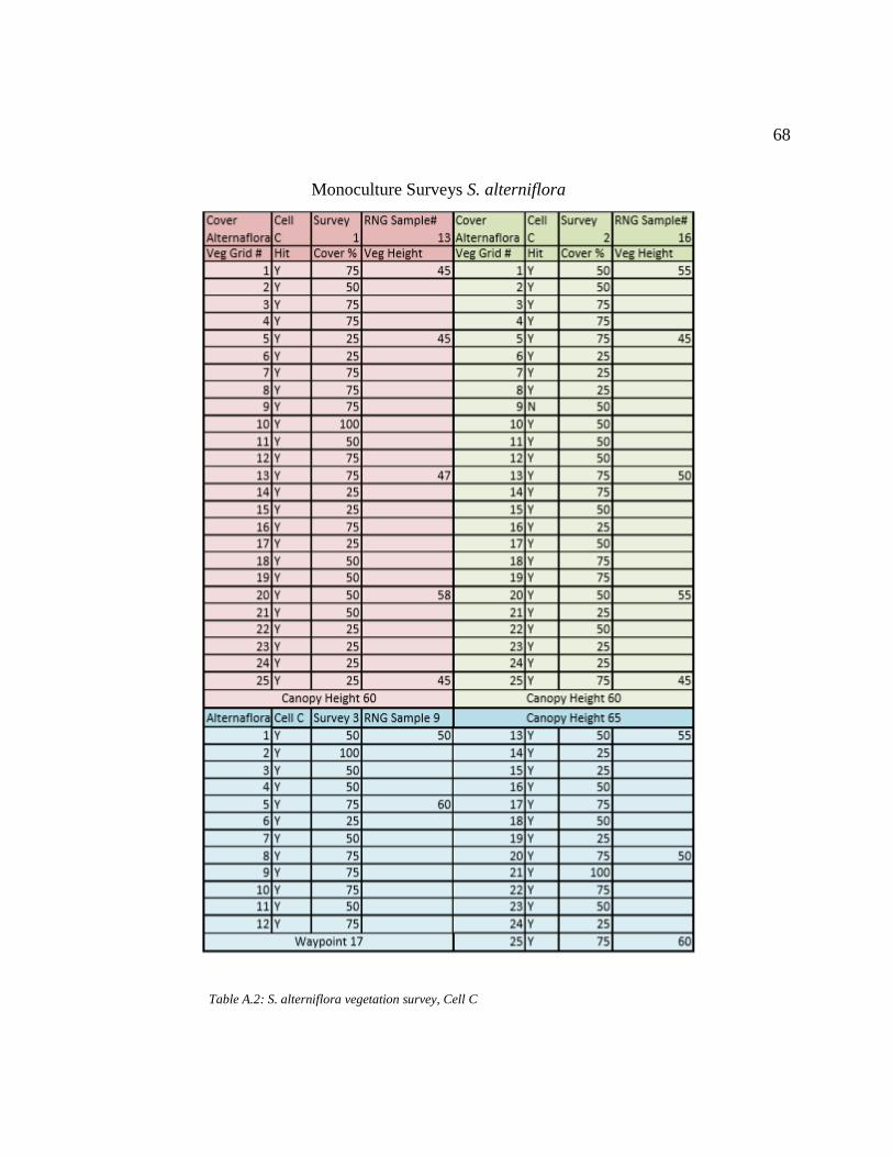
68
Table A.2: S. alterniflora vegetation survey, Cell C
Monoculture Surveys S. alterniflora

69
Table A.3: S. alterniflora vegetation survey, Cell B
Monoculture Surveys S. alterniflora

70
Table A.4: S. patens vegetation survey, Cell A
Monoculture Surveys S. patens

71
Table A.5: S. patens vegetation survey, Cell C
Monoculture Surveys S. patens
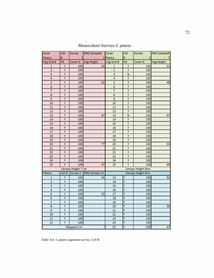
72
Table A.6: S. patens vegetation survey, Cell B
Monoculture Surveys S. patens

73
Table A.7: G. geradii alive vegetation survey, Cell A
Monoculture Surveys J. geradii alive

74
Table A.8: G. geradii alive vegetation survey, Cell C
Monoculture Surveys J. geradii alive
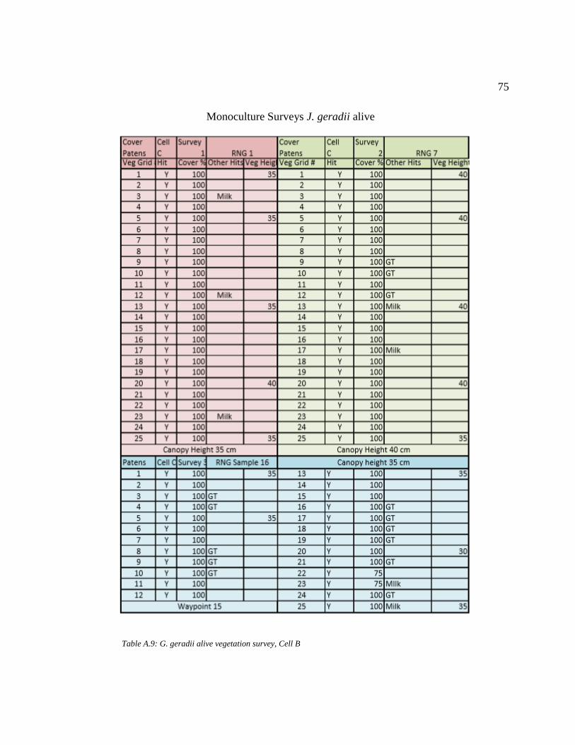
75
Table A.9: G. geradii alive vegetation survey, Cell B
Monoculture Surveys J. geradii alive

76
Table A.10: G. geradii dead vegetation survey, Cell A
Monoculture Surveys J. geradii dying
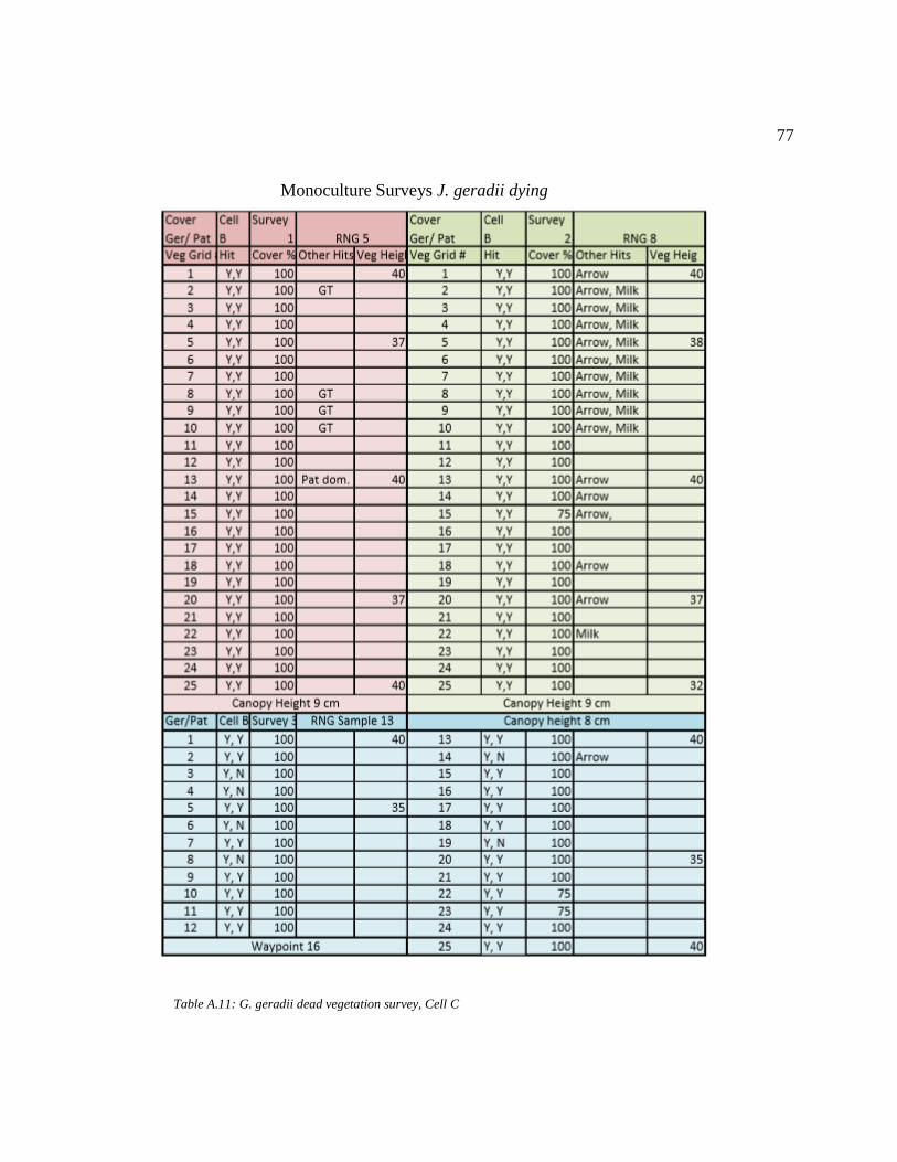
77
Table A.11: G. geradii dead vegetation survey, Cell C
Monoculture Surveys J. geradii dying
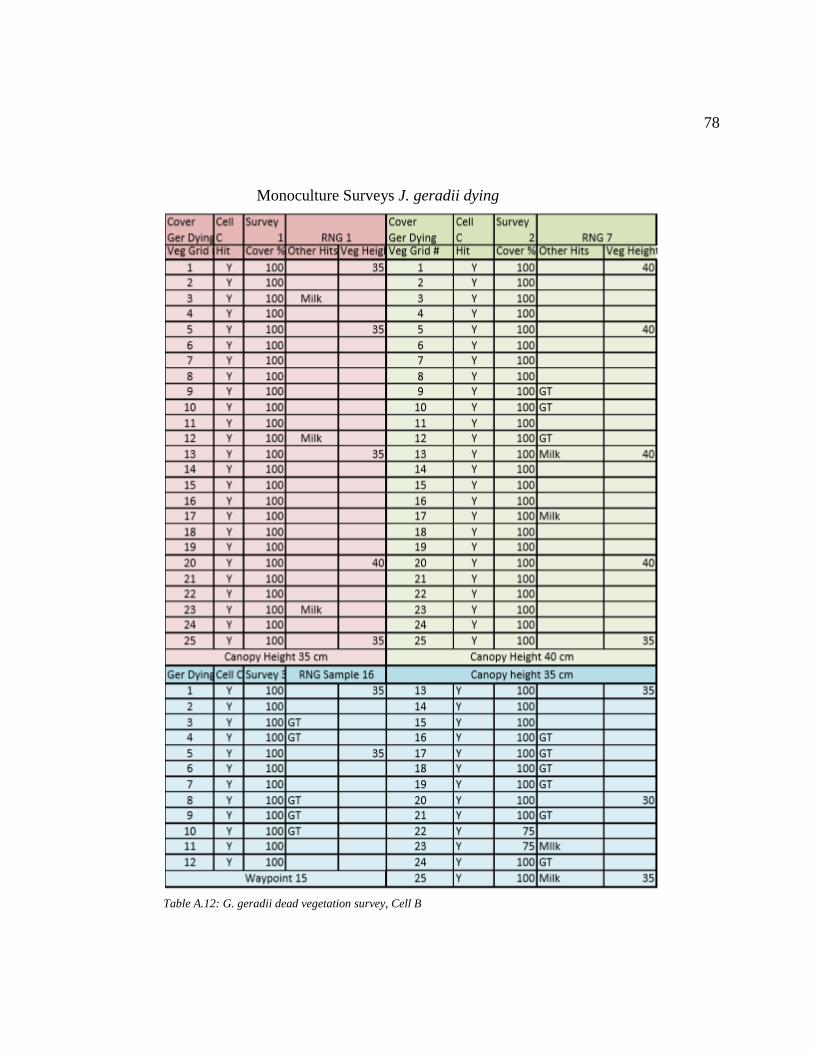
78
Table A.12: G. geradii dead vegetation survey, Cell B
Monoculture Surveys J. geradii dying

79
Figure A.13 (A-F): Cell B S. alterniflora (A-C) and S. patens (D-F) survey images
A
B
C
D
E
F

80
A
B
C
D
E
F
Figure A.14 (A-F): Cell C S. alterniflora (A-C) and S. patens (D-F) survey images
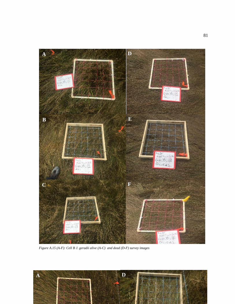
81
A
B
C
D
E
F
Figure A.15 (A-F): Cell B J. geradii alive (A-C) and dead (D-F) survey images
A D

82

83
Figure A.17: Pix4D Report for 50 and 70m multispectral flights
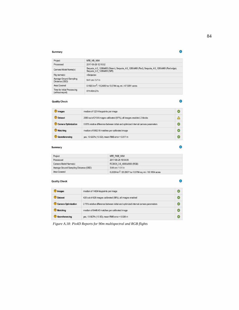
84
Figure A.18: Pix4D Reports for 90m multispectral and RGB flights


![FY18 RWDC State Unmanned Aerial System Challenge ... · Unmanned Aerial System Challenge: Practical Solutions to ... , Real World Design Challenge ... , unmanned aerial vehicle [UAV])](https://img.pdfslide.us/doc/110x75/5ae85cfb7f8b9a8b2b8fe5e5/fy18-rwdc-state-unmanned-aerial-system-challenge-aerial-system-challenge-practical.jpg)